Birman-Wenzl-Murakami Algebra, Topological parameter and Berry phase

Abstract

In this paper, a $3\times 3$-matrix representation of Birman-Wenzl-Murakami(BWM) algebra has been presented. Based on which, unitary matrices $A(\theta,\varphi_{1},\varphi_{2})$ and $B(\theta,\varphi_{1},\varphi_{2})$ are generated via Yang-Baxterization approach. A Hamiltonian is constructed from the unitary $B(\theta,\varphi)$ matrix. Then we study Berry phase of the Yang-Baxter system, and obtain the relationship between topological parameter and Berry phase.

I Introduction

To the best of our knowledge, the Yang-Baxter equation (YBE) was initiated in solving the one-dimensional $\delta$-interecting models ye and the statistical models be . Braid algebra and Temperley-Lieb algebra (TLA) tla have been widely used in the construction of YBE solutions kve ; kk ; yg ; bob ; bk ; yql and have been introduced to the field of quantum information, quantum computation and topological computation ayk ; kl ; frw ; cxg1 ; sw ; knot . The Birman-Wenzl-Murakami (BWM) algebra bwma which contain two subalgebra (Braid algebra and TLA) was first defined and independently studied by Birman, Wenzl and Murakami. Very recently tlaknot , S.Abramsky demonstrate the connections from knot theory to logic and computation via quantum mechanics. But, the physical meaning of the topological parameter $d$ (describing the single loop in topology) is still unclear.

The geometrical phase b , such as Berry phase, is an important concept in quantum mechanics aa ; spe ; sb ; ts ; w ; bpxxz . In recent years, numerous works have been attributed to Berry phase bmk , because of its possible applications to quantum computation (the so-called geometric quantum computation) jve ; dcz ; ww ; eeh . Quantum logic gates based on geometric phases have been certified in both nuclear magnetic resonance jve and ion trap based on quantum information architectures gpit . The Ref. jve pointed out geometric phases have potential fault tolerance when applied to quantum information processing. In 2007, Leek, P.J. et al. bpss illustrated the controlled accumulation of a geometric phase, Berry phase, in a superconducting qubit.

The Ref. hxg applied TLA as a bridge to recast 4-dimensional YBE into its 2-dimensional counterpart. The 2-dimensional YBE have an important application value in topological quantum computation tqc1 ; tqc2 . To date, few studies have reported 3-dimensional YBE which may have potential application values in topological quantum computation. The motivation of this paper is twofold: one is that we structure 3-dimensional YBE , the other is to study the physical meaning of topological parameter $d$ from Berry phase. This paper is organized as follows: In Sec. 2, we introduce a specialized type BWM algebra, and present a $3\times 3$-matrix representation of BWM algebra. In Sec. 3, we obtain unitary matrices $A(\theta,\varphi_{1},\varphi_{2}),B(\theta,\varphi_{1},\varphi_{2})$ via Yang-Baxterization approach. Based on the solution, a Hamiltonian of the Yang-Baxter system is constructed, finally we study the Berry phase of this system. We end with a summary.

II BWM Algebra

As we know the Braid relations are

$$\left\{\begin{aligned} &b_{i}b_{i\pm 1}b_{i}=b_{i\pm 1}b_{i}b_{i\pm 1},\\ &b_{i}b_{j}=b_{j}b_{i},\ |i-j|\geq 2,\\ \end{aligned}\right.$$ (1)

where $b_{i}=\stackrel{{\scriptstyle 1}}{{I}}\otimes\cdots\otimes\stackrel{{\scriptstyle i-1}}{{I}}\otimes b\otimes\stackrel{{\scriptstyle i+2}}{{I}}\otimes\cdots$. When we just consider three tensor product space, the Braid relations becomes

$$b_{12}b_{23}b_{12}=b_{23}b_{12}b_{23},$$ (2)

where $b_{12}=b\otimes I,b_{23}=I\otimes b$, $b$-matrix is a $N^{2}\times N^{2}$ matrix acted on the tensor product space $\nu\otimes\nu$, where $N$ is the dimension of $\nu$. It is also well known that the braid relation can be reduced to a $N$-dimensional braid relation $(b_{12}\rightarrow A,b_{23}\rightarrow B)$

$$ABA=BAB.$$ (3)

Like this reduced method, we easily obtain $N$-dimensional reduced BWM-algebra relations from classical BWM-algebra relations. The BWM algebra bwma ; cgx ; gx2 ; j is generated by the unit $I$, the braid operators $S_{i}$ and the TLA operators $E_{i}$ and depends on two independent parameters $\omega$ and $\sigma$. Let us take the BWM relations as follows.

$$\left\{\begin{aligned} &S_{i}-S_{i}^{-1}=\omega(I-E_{i}),\\ &S_{i}S_{i\pm 1}S_{i}=S_{i\pm 1}S_{i}S_{i\pm 1},\ S_{i}S_{j}=S_{j}S_{i},|i-j|\geq 2,\\ &E_{i}E_{i\pm 1}E_{i}=E_{i},\ E_{i}E_{j}=E_{j}E_{i},\ |i-j|\geq 2,\\ &E_{i}S_{i}=S_{i}E_{i}=\sigma E_{i},\\ &S_{i\pm 1}S_{i}E_{i\pm 1}=E_{i}S_{i\pm 1}S_{i}=E_{i}E_{i\pm 1},\\ &S_{i\pm 1}E_{i}S_{i\pm 1}=S_{i}^{-1}E_{i\pm 1}S_{i}^{-1},\\ &E_{i\pm 1}E_{i}S_{i\pm 1}=E_{i\pm 1}S_{i}^{-1},\ S_{i\pm 1}E_{i}E_{i\pm 1}=S_{i}^{-1}E_{i\pm 1},\\ &E_{i}S_{i\pm 1}E_{i}=\sigma^{-1}E_{i},\\ &E_{i}^{2}=\left(1-\frac{\sigma-\sigma^{-1}}{\omega}\right)E_{i},\end{aligned}\right.$$ (4)

where $0\neq d=\left(1-\frac{\sigma-\sigma^{-1}}{\omega}\right)\in\mathbb{C}$ is a topological parameter in knot theory which does not depend on the sites of the lattices.

By reducing to the $N$-dimensional space $(S_{12}\rightarrow A,S_{23}\rightarrow B,E_{12}\rightarrow E_{A},E_{23}\rightarrow E_{B})$, we have:

$$\left\{\begin{aligned} &A-A^{-1}=\omega(I-E_{A}),\ B-B^{-1}=\omega(I-E_{B}),\\ &ABA=BAB,\\ &E_{A}E_{B}E_{A}=E_{A},\ E_{B}E_{A}E_{B}=E_{B},\\ &E_{A}A=AE_{A}=\sigma E_{A},\ E_{B}B=BE_{B}=\sigma E_{B},\\ &ABE_{A}=E_{B}AB=E_{B}E_{A},\ BAE_{B}=E_{A}BA=E_{A}E_{B},\\ &AE_{B}A=B^{-1}E_{A}B^{-1},\ BE_{A}B=A^{-1}E_{B}A^{-1},\\ &E_{A}E_{B}A=E_{A}B^{-1},\ E_{B}E_{A}B=E_{B}A^{-1},\\ &AE_{B}E_{A}=B^{-1}E_{A},\ BE_{A}E_{B}=A^{-1}E_{B},\\ &E_{A}BE_{A}=\sigma^{-1}E_{A},\ E_{B}AE_{B}=\sigma^{-1}E_{B},\\ &E_{A}^{2}=(1-\frac{\sigma-\sigma^{-1}}{\omega})E_{A},\ E_{B}^{2}=(1-\frac{\sigma-\sigma^{-1}}{\omega})E_{B},\end{aligned}\right.$$ (5)

where $A,B$ satisfy the $N$-dimensional Braid relation (3), $E_{A},E_{B}$ satisfy the $N$-dimensional TLA relations

$$\left\{\begin{aligned} &E_{A}E_{B}E_{A}=E_{A},\ E_{B}E_{A}E_{B}=E_{B},\\ &E_{A}^{2}=dE_{A},\ E_{B}^{2}=dE_{B},\end{aligned}\right.$$ (6)

It is interesting that Eq.(4) and Eq.(5) have the same topological parameter $d$.

In this paper, the $A$-matrix, $B$-matrix, $E_{a}$-matrix, $E_{b}$-matrix, $A(x)$-matrix and $B(x)$-matrix are $3\times 3$ matrices acting on the 3-dimensional space. To the TLA relations (6), we assume $E_{A}$ and $E_{B}$ possess the same eigenvalues $d$ and 0. We assume $E_{A}$ is a diagonal matrix as following

$$E_{A}=\left(\begin{array}[]{>{\displaystyle}l>{\displaystyle}c>{\displaystyle}r}0&0&0\\ 0&d&0\\ 0&0&0\end{array}\right).$$ (7)

After tedious calculation,we obtain

$$E_{B}=\left(\begin{array}[]{>{\displaystyle}l>{\displaystyle}c>{\displaystyle}r}\frac{d^{2}-d-1}{d}&\frac{\sqrt{d^{2}-d-1}}{d}e^{i\varphi_{1}}&-\frac{\sqrt{d^{2}-d-1}}{\sqrt{d}}e^{i(\varphi_{1}+\varphi_{2})}\\ \frac{\sqrt{d^{2}-d-1}}{d}e^{-i\varphi_{1}}&\frac{1}{d}&-\frac{e^{i\varphi_{2}}}{\sqrt{d}}\\ -\frac{\sqrt{d^{2}-d-1}}{\sqrt{d}}e^{-i(\varphi_{1}+\varphi_{2})}&-\frac{e^{-i\varphi_{2}}}{\sqrt{d}}&1\end{array}\right).$$ (8)

It is worth to mention that $E_{B}=UE_{A}U^{-1}$, and $U$ is a unitary transformation matrix as follows

$$U=\left(\begin{array}[]{>{\displaystyle}l>{\displaystyle}c>{\displaystyle}r}\frac{1}{(d-1)d}&-\frac{\sqrt{d^{2}-d-1}}{d}e^{i\varphi_{1}}&-\frac{\sqrt{d^{2}-d-1}}{\sqrt{d}(d-1)}e^{i(\varphi_{1}+\varphi_{2})}\\ \frac{\sqrt{d^{2}-d-1}}{d}e^{-i\varphi_{1}}&-\frac{1}{d}&\frac{e^{i\varphi_{2}}}{\sqrt{d}}\\ \frac{\sqrt{d^{2}-d-1}}{\sqrt{d}(d-1)}e^{-i(\varphi_{1}+\varphi_{2})}&\frac{e^{-i\varphi_{2}}}{\sqrt{d}}&-\frac{d-2}{d-1}\end{array}\right),$$ (9)

where $d$, $\varphi_{1}$ and $\varphi_{2}$ are reals. The parameter $d$ is the so-called topological parameter. For simplicity, we just consider the case of $d>0$ in this paper.

The Ref. cgx has explored $S_{i}$ have 3 different eigenvalues$(q,-q^{-1},q^{-2})$ in the BWM-algebra (i.e. Eq.(4)). The same as $E_{A}$ and $E_{B}$, we assume $A$ and $B$ have the same eigenvalues$(q,-q^{-1},q^{-2})$. The simplest $A$ is

$$A=\left(\begin{array}[]{>{\displaystyle}l>{\displaystyle}c>{\displaystyle}r}q&0&0\\ \\ 0&q^{-2}&0\\ \\ 0&0&-q^{-1}\end{array}\right),$$ (10)

using the unitary transformation matrix $U$, we have

$$B=UAU^{-1}=\left(\begin{array}[]{>{\displaystyle}l>{\displaystyle}c>{\displaystyle}r}\frac{1}{q^{4}(d-1)d}&\frac{\sqrt{d^{2}-d-1}}{dq}e^{i\varphi_{1}}&-\frac{\sqrt{d^{2}-d-1}}{q^{2}(d-1)\sqrt{d}}e^{i(\varphi_{1}+\varphi_{2})}\\ \frac{\sqrt{d^{2}-d-1}}{dq}e^{-i\varphi_{1}}&\frac{q^{2}}{d}&\frac{q}{\sqrt{d}}e^{i\varphi_{2}}\\ -\frac{\sqrt{d^{2}-d-1}}{q^{2}(d-1)\sqrt{d}}e^{-i(\varphi_{1}+\varphi_{2})}&\frac{q}{\sqrt{d}}e^{-i\varphi_{2}}&\frac{d-2}{d-1}\end{array}\right),$$ (11)

where $d=q^{-1}+1+q$ and the parameter $q$ is real. The matrices $A$ and $B$ satisfy the braid relation (i.e. Eq(3)). Towards braid relation, in some models $\varphi_{i},(i=1,2)$, may have a physical significance of magnetic flux. In the papercxg1 , it has been shown the parameters $\varphi_{i}$’s are related to Berry phase.

Then we can verify that $\{I,A,E_{A},B,E_{B}\}$ satisfy the reduced BWM-algebra (i.e. Eq.(5)), with $d=q^{-1}+1+q$. Here we have set $\omega=q-q^{-1}$and $\sigma=q^{-2}$. It is interesting that $A,B,E_{A},E_{B}$ are Hermitian matrices, and have the same similar transformation $B=UAU^{-1},E_{B}=UE_{A}U^{-1}$, where $U$ is unitary (i.e. $U^{{\dagger}}=U^{-1}$).

III Yang-Baxterization, Hamiltonian, Berry phase

In this section, A Hamiltonian is constructed from the unitary $B(\theta,\varphi)$ matrix. Then we study the Berry phase of the Yang-Baxter system, and obtain the relationship between the topological parameter and the Berry phase. We first explain the basic formula of YBE. The Yang-Baxter matrix $\check{R}$ is a $N^{2}\times N^{2}$ matrix acting on the tensor product space $\nu\otimes\nu$, where $N$ is the dimension of $\nu$. Such a matrix $\check{R}$ satisfies the relativistic YBEhxg as follows

$$\check{R}_{12}(u)\check{R}_{23}(\frac{u+v}{1+\beta^{2}uv})\check{R}_{12}(v)=\check{R}_{23}(v)\check{R}_{12}(\frac{u+v}{1+\beta^{2}uv})\check{R}_{23}(u).$$ (12)

In this paper, we focus on 3-dimensional space. The reduced relativistic YBE reads

$$A(u)B(\frac{u+v}{1+\beta^{2}uv})A(v)=B(v)A(\frac{u+v}{1+\beta^{2}uv})B(u).$$ (13)

Let the unitary Yang-Baxter matrix take the form

$$\left\{\begin{aligned} &A(u)=\rho(u)(I+F(u)E_{A})\\ &B(u)=\rho(u)(I+F(u)E_{B}).\end{aligned}\right.$$ (14)

Following Xue et al. wx1 , we obtain

$$\left\{\begin{aligned} &F(u)=\frac{e^{-2i\theta}-1}{d},\\ &e^{-2i\theta}=\frac{\beta^{2}u^{2}+2i\varepsilon\beta u\sqrt{d^{2}/(4-d^{2})}+1}{\beta^{2}u^{2}-2i\varepsilon\beta u\sqrt{d^{2}/(4-d^{2})}+1},\end{aligned}\right.$$ (15)

where the new parameter $\theta$ is real. Let $\rho(u)=e^{i\theta}$. The Yang-Baxter matrix can be rewritten in the following form

$$\left\{\begin{aligned} &A(\theta,\varphi_{1},\varphi_{2})=e^{i\theta}I-f(\theta)E_{A},\\ &B(\theta,\varphi_{1},\varphi_{2})=e^{i\theta}I-f(\theta)E_{B},\end{aligned}\right.$$ (16)

where $f(\theta)=2i\sin{\theta}/d$.

The Yang-Baxter matrix depends on three parameters: the first is $\theta$ ($\theta$ is time-independent); the others are $\varphi_{i},(i=1,2)$ contained in the matrix $E$. In physics the parameter $\varphi_{1}$ and $\varphi_{2}$ are flux which depends on time $t$. Usually take $\varphi_{i}=\omega_{i}t,(i=1,2)$ and $\omega_{i}$ are the frequency. Operators $A(\theta,\varphi_{1},\varphi_{2})$ and $B(\theta,\varphi_{1},\varphi_{2})$, satisfying $B(\theta,\varphi_{1},\varphi_{2})=UA(\theta,\varphi_{1},\varphi_{2})U^{-1}$, are unitary operators $(A(\theta,\varphi_{1},\varphi_{2})^{{\dagger}}=A(\theta,\varphi_{1},\varphi_{2})^{-1},B(\theta,\varphi_{1},\varphi_{2})^{{\dagger}}=B(\theta,\varphi_{1},\varphi_{2})^{-1})$.

To simplify the following discussion, we will restrict attention to the case $\varphi_{1}=-\varphi_{2}=\varphi$. Following Ge et al. cxg1 , we can obtain Yang Baxter Hamiltonian through the Schr$\ddot{o}$dinger evolution of the states

$$\hat{H}=i\hbar\frac{\partial B(\theta,\varphi)}{\partial t}B^{{\dagger}}(\theta,\varphi),$$ (17)

where $\varphi$ be time dependent as $\varphi=\omega t$ and $\theta$ be time independent.

For convenience, we introduce the Gell-Mann matrices $I_{\lambda}$gm , a basis for $su(3)$ algebra. Such matrices satisfy $[I_{\lambda},I_{\mu}]=if_{\lambda\mu\nu}I_{\nu},(\lambda,\mu,\nu=1,2,...,8)$, where $f_{\lambda\mu\nu}$ are the structure constants of $su(3)$. We denote $I_{\pm}=I_{1}\pm iI_{2}$, $V_{\pm}=I_{4}\mp iI_{5}$, $U_{\pm}=I_{6}\pm iI_{7}$ and $Y=\frac{2}{\sqrt{3}}I_{8}$. Let

$$\left\{\begin{aligned} S_{+}=&\zeta(-i(d^{2}-d-1)^{1/2}(e^{-i\theta}+2i\sin{\theta}d^{-2})I_{+}+id^{1/2}(e^{-i\theta}+2i\sin{\theta}d^{-2})U_{-}),\\ S_{-}=&\zeta(i(d^{2}-d-1)^{1/2}(e^{i\theta}-2i\sin{\theta}d^{-2})I_{-}-id^{1/2}(e^{i\theta}-2i\sin{\theta}d^{-2})U_{+}),\\ S_{3}=&\frac{1}{2}\big{[}(1+d-d^{2})(1-d^{2})^{-1}(\frac{I}{3}+\frac{Y}{2}+I_{3})-(\frac{I}{3}+\frac{Y}{2}-I_{3})-d(1-d^{2})^{-1}(\frac{I}{3}-Y)\\ &+d^{1/2}(d^{2}-d-1)^{1/2}(1-d^{2})^{-1}(V_{-}+V_{+})\big{]},\end{aligned}\right.$$ (18)

where $\zeta=\frac{d^{2}}{\sqrt{(d^{2}-1)(d^{4}-4(d^{2}-1)\sin^{2}{\theta})}}$. These operators satisfy the $su(2)$ algebra relations $([S_{+},S_{-}]=2S_{3},[S_{3},S_{\pm}]=\pm S_{\pm},(S_{\pm})^{2}=0,S_{\pm}=S_{1}\pm iS_{2})$.

In terms of the operators(18), the Hamiltonian Eq.(17) can be recast as following

$$\hat{H}= -4\omega\hbar\sin{\theta}(d^{2}-1)^{1/2}d^{-2}(\sin{\alpha}\cos{\beta}S_{1}+\sin{\alpha}\sin{\beta}S_{2}+\cos{\alpha}S_{3}).$$ (19)

Its eigenvalues are $E_{0}=0,E_{\pm}=\mp\omega\hbar\cos{\alpha}$, where $\cos{\alpha}=\frac{2\sin{\theta}\sqrt{d^{2}-1}}{d^{2}}$, $\beta=\varphi$, here $d\geq 1$. By the way, its Casimir operator is $\kappa=\frac{1}{2}(S_{+}S_{-}+S_{-}S_{+})+S_{3}^{2}$. It is easy to find the eigenvalues of $\kappa$ are $\frac{1}{2}(\frac{1}{2}+1)=\frac{3}{4}$ and $0(0+1)=0$, which correspond to spin-1/2 and spin-0. According to the definition of Berry phase, when $\varphi(t)$ evolves adiabatically from 0 to $2\pi$, the corresponding Berry phase is

$$\gamma_{\alpha}=i\int_{0}^{T}\langle\Psi_{\alpha}|\frac{\partial}{\partial t}|\Psi_{\alpha}\rangle dt.$$ (20)

Noting that Hamiltonian returns to its original form after the time $T=2\pi/\omega$, we easily obtain the corresponding Berry phases of this Yang-baxter system

$$\left\{\begin{aligned} &\gamma_{0}=0,\\ &\gamma_{\pm}=\pm\pi(1-\cos{\alpha})=\pm\frac{\Omega}{2},\end{aligned}\right.$$ (21)

where $\Omega=2\pi(1-\cos{\alpha})$ is the solid angle enclosed by the loop on the Bloch sphere. The system also equals to spin-$1/2$ system and spin-$0$ system. Substituting $\cos{\alpha}=\frac{2\sin{\theta}\sqrt{d^{2}-1}}{d^{2}}$ into Eq.(21), we obtain $\gamma_{\pm}=\pm\pi(1-\frac{2\sin{\theta}\sqrt{d^{2}-1}}{d^{2}})$. Substituting $\theta$ with $\frac{\pi}{2}-\theta$, we rewrite Berry phase as follows

$$\gamma_{\pm}=\pm\pi(1-\frac{2\cos{\theta}\sqrt{d^{2}-1}}{d^{2}}).$$ (22)

It is worth mentioning that in some paperscxg1 , the Berry phase $\gamma_{\pm}=\pm\pi(1-\cos{\theta})$ of Yang-Baxter system only depends on the spectral parameter $\theta$. It is interesting that in our paper, the Berry phases(22) not only depends on the spectral parameter $\theta$, but also depends on the topological parameter $d$. The Berry phase (Eq.(22)) reduce to $\gamma_{\pm}=\pm\pi(1-\cos{\theta})$ if $d=\sqrt{2}$. The FIG. 1, which corresponds to the Berry phase $\gamma_{+}$. The FIG. 1 illustrate the Berry phases Eq.(22) versus the spectral parameter $\theta$ and the topological parameter $d$. The FIG. 1 illustrate the Berry phase $\gamma_{+}$ versus the spectral parameter $\theta$, when $d$ choice specific values. It is demonstrated that the Berry phase $\gamma_{+}$ is maximum (minimum) at parameter $\theta=(2n+1)\pi$ ($\theta=2n\pi$), for a given definit value of $d$. Where $n$ is integer. The maximum (minimum) of $\gamma_{+}$ is $\pi(1+\frac{2\sqrt{d^{2}-1}}{d^{2}})$ ($\pi(1-\frac{2\sqrt{d^{2}-1}}{d^{2}})$). As $d$ increase, the maximum of $\gamma_{+}$ decreases, the minimum of $\gamma_{+}$ increases. The Berry phase $\gamma_{+}$ tend to a constant value $\pi$, with $d$ approaches infinity.

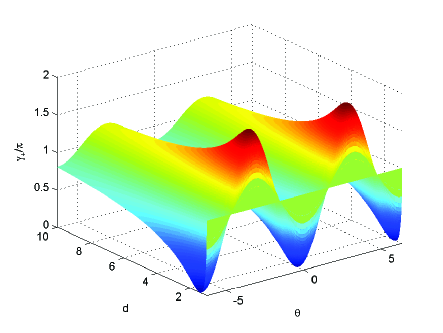
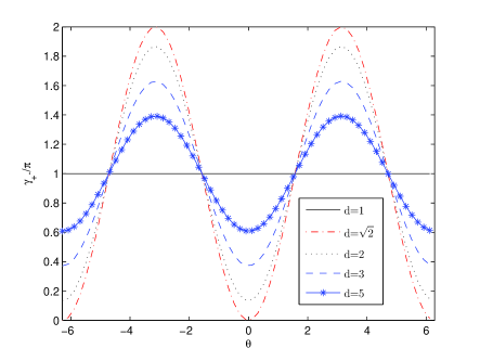
Figure 1: (The left figure shows the Berry phase $\gamma_{+}=\pi(1-\frac{2\cos{\theta}\sqrt{d^{2}-1}}{d^{2}})$ versus the the topological parameter $d$ and the spectral parameter $\theta$. The right figure, the sectional drawings have also provided with the same values of parameters. $d=1$ (solid line), $d=\sqrt{2}$ (dot-dashed line), $d=2$ (dotted line), $d=3$ (dashed line), $d=5$ (star line).)

IV Summary

In this paper we presented BWM-algebra $(A,\ B,\ E_{A},\ E_{B})$ and solution of YBE $(A(\theta,\varphi_{1},\varphi_{2}),\ B(\theta,\varphi_{1},\varphi_{2}))$ in 3-dimensional representation which satisify $B=UAU^{-1}$, $E_{B}=UE_{A}U^{-1}$ and $B(\theta,\varphi_{1},\varphi_{2})=UA(\theta,\varphi_{1},\varphi_{2})U^{-1}$. The evolution of the Yang-Baxter system is explored by constructing a Hamiltonian from the unitary $B(\theta,\varphi)$ matrix. We study the Berry phase of the Yang-Baxter system, and obtain the relationship between topological parameter and Berry phase $\gamma_{\pm}=\pm\pi(1-\frac{2\cos{\theta}\sqrt{d^{2}-1}}{d^{2}})$. Then we compare the Berry phase of Yang-Baxter system in Ref.cxg1 with us, and find the topological parameter d plays a deformation role in the Berry phase. We have been discussing in this paper is still an open problem that will require a deal of further investigations.

V Acknowledgments

This work was supported in part by NSF of China (Grant No.10875026)

References

- (1) Yang, C.N.: Some Exact Results for the Many-Body Problem in one Dimension with Repulsive Delta-Function Interaction. Phys. Rev. Lett. 19, 1312 (1967); Yang, C.N.: S matrix for the one-dimensional N body problem with repulsive or attractive delta function interaction. Phys. Rev. 168, 1920 (1968).
- (2) Baxter, R.J.: it Exactly Solved Models in Statistical Mechanics. New York: Academic (1982); Baxter, R.J.: Partition function of the Eight-Vertex lattice model. Ann. Phys. 70, 193 (1972).
- (3) Temperley, H.N.V., Lieb, E.H.: Relations between the ’Percolation’ and ’Colouring’ Problem and other Graph-Theoretical Problems Associated with Regular Planar Lattices: Some Exact Results for the ’Percolation’ Problem. Proc. Roy. Soc. London, A 322, 251 (1971).
- (4) Korepin, V.E., Bogoliubov, N.M., Izergin, A.G.: Quantum Inverse Scattering Method and Correlation Functions. Cambridge University Press (1993)
- (5) Kauffman, L.H.: Knots and Physics. Singapore: World Scientific Publ Co Ltd. (1991)
- (6) Yang. C.N., Ge. M.L.,et al.: Braid Group, Knot Theory and Statistical Mechanics (I and II). SingaporeWorld Scientific Publ Co Ltd. (1989) and (1994).
- (7) Baxter, R.J.: The inversion relation method for some two-dimensional exactly solved models in lattice statistics. J.Stat.Phys. 28, 1 (1982); Owczarek, A.L., Baxter, R.J.: A Class of Interaction-Round-a-Face Models and Its Equivalence with an Ice-Type Model. J.Stat.Phys. 49, 1093 (1987); Batchelor, M.T., Barber, M.N.: Spin-s quantum chains and Temperley-Lieb algebras. J. Phys. A 23, L15 (1990).
- (8) Batchelor, M.T., Kuniba, A.: Temperley-Lieb lattice models arising from quantum groups. J. Phys. A 24, 2599 (1991).
- (9) Li, Y.Q.: Yang Baxterization.J. Math. Phys. 34, 2 (1993).
- (10) Kauffman, L.H., Lomonaco Jr, S.J.: Braiding Operators are Universal Quantum Gates. New J. Phys. 6, 413 (2004).
- (11) Kitaev, A.Y.:Fault-tolerant quantum computation by anyons. Ann. Phys. 303, 2 (2003).
- (12) Franko, J., Rowell, E.C., Wang, Z.: Extraspecial 2-Groups and Images of Braid Group Representations. J. Knot Theor Ramif. 15, 413 (2006).
- (13) Chen, J.L., Xue, K., Ge, M.L.: Braiding transformation, entanglement swapping, and Berry phase in entanglement space. Phys. Rev. A. 76, 042324 (2007); Chen, J.L., Xue, K., Ge, M.L.: Berry phase and quantum criticality in Yang-Baxter systems. Annals of Physics 323, 2614 (2008).
- (14) Sun, C.F., et al.: Thermal entanglement in the two-qubit systems constructed from the Yang-Baxter R-matrix. International Journal of Quantum Information 7, 879 (2009).
- (15) Wadati, M., Deguchi, T., Akutsu, Y.: Exactly solvable models and knot theory. Phys. Rep. 180, 247 (1989).
- (16) Birman .J, Wenzl .H.: Braids, link polynomials and a new algebra. Trans. A.M.S. 313, 249 (1989); Murakami .J.: The Kauffman Polynomial of Links and Representation Theory. Osaka J. Math. 24, 745 (1987).
- (17) Abramsky, S.: Temperley-Lieb Algebra: From Knot Theory to Logic and Computation via Quantum Mechanics. e-print quant-ph/0910.2737.
- (18) Berry, M.V.: Quantal phase factors accompanying adiabatic changes. Proc. R. Soc. Lond. Ser. A 392, 45 (1984).
- (19) Aharonov, Y., Anandan, J.: Phase change during a cyclic quantum evolution. Phys. Rev. Lett. 58, 1593 (1987).
- (20) Sjöqvist, E., Pati, A.K., Ekert, A., Anandan, J.S., Ericsson, M., Oi, D.K.L., Vedral, V.: Geometric Phases for Mixed States in Interferometry. Phys. Rev. Lett. 85, 2845 (2000).
- (21) Samuel, J., Bhandari, R.: General Setting for Berry’s Phase. Phys. Rev. Lett. 60, 2339 (1988).
- (22) Tong, D.M., Sjöqvist, E., Kwek, L.C., Oh, C.H.: Kinematic Approach to the Mixed State Geometric Phase in Nonunitary Evolution. Phys. Rev. Lett. 93, 080405 (2004).
- (23) Wilczek, F., Zee, A.: Appearance of Gauge Structure in Simple Dynamical Systems. Phys. Rev. Lett. 52, 2111 (1984).
- (24) Korepin, V.E., Wu, A.C.T.: Adiabatic Transport Properties and BERRY S Phase in Heisenberg-Ising Ring. International Journal of Modern Physics B 5, 497 (1991).
- (25) Appelt, S., Wckerle, G., Mehring, M.: Deviation from Berry s adiabatic geometric phase in a 131Xe nuclear gyroscope. Phys. Rev. Lett. 72, 3921 (1994).
- (26) Jones, J., Vedral, V., Ekert, A., Castagnoli, G.: Geometric quantum computation using nuclear magnetic resonance. Nature 403, 869 (2000).
- (27) Duan, L.M., Cirac, J.I., Zoller, P.: Geometric Manipulation of Trapped Ions for Quantum Computation. Science 292, 1695 (2001).
- (28) Wootters, W.K.: Entanglement of Formation of an Arbitrary State of Two Qubits. Phys. Rev. Lett. 80, 2245 (1998).
- (29) Ekert, A., Ericsson, M., Hayden, P., Inamori, H., Jones, J.A., Oi, D.K.L., Vedral, V.: Geometric quantum computation. J. Mod. Opt. 47, 2501 (2000).
- (30) Leibfried, D., et al.: Experimental demonstration of a robust, high-fidelity geometric two ion-qubit phase gate. Nature 422, 412 (2003).
- (31) Leek, P.J., et al.: Observation of Berry’s Phase in a Solid-State Qubit. science 318, 1889 (2007).
- (32) Hu, S.W., Xue, K., Ge, M.L. Optical simulation of the Yang-Baxter equation. Phys. Rev. A 78, 022319 (2008).
- (33) Nayak, C., Simon, S.H., Stern, A., Freedman, M., Sarma, S.D. Non-Abelian anyons and topological quantum computation. Rev. Mod. Phys. 80, 1083 (2008).
- (34) Hikami, K.: Skein theory and topological quantum registers: Braiding matrices and topological entanglement entropy of non-Abelian quantum Hall states. Ann. Phys. 323, 1729 (1987).
- (35) Cheng, Y.,Ge, M.L., Xue, K.: Yang-Baxterization of braid group representations. Commun Math Phys. 136, 195 (1991).
- (36) Ge, M.L., Xue, K.: Trigonometric Yang-Baxterization of colored R-matrix. J. Phys. A: Math. 26, 281 (1993).
- (37) Jones, V.F.R.: On a certain value of the Kauffman polynomial. Commun Math Phys. 125, 459 (1987).
- (38) Wang, G.C., et al.: Temperley-Lieb algebra, Yang-Baxterization and universal gate. Quantum Information Processing. 9, 699 (2009).
- (39) Pfeifer, W.: The Lie Algebras , An Introduction. Birkhauser Verlag (2003).