Arnold Tongues and Feigenbaum Exponents of the Rational Mapping for $Q$-State Potts Model on Recursive Lattice: $Q<2$

Abstract

We considered $Q$-state Potts model on Bethe lattice in presence of external magnetic field for $Q<2$ by means of recursion relation technique. This allows to study the phase transition mechanism in terms of the obtained one dimensional rational mapping. The convergence of Feigenabaum $\alpha$ and $\delta$ exponents for the aforementioned mapping is investigated for the period doubling and three cyclic window. We regarded the Lyapunov exponent as an order parameter for the characterization of the model and discussed its dependence on temperature and magnetic field. Arnold tongues analogs with winding numbers $\mathrm{w}=1/2$, $\mathrm{w}=2/4$ and $\mathrm{w}=1/3$ (in the three cyclic window) are constructed for $Q<2$. The critical temperatures of the model are discussed and their dependence on $Q$ is investigated. We also proposed an approximate method for constructing Arnold tongues via Feigenbaum $\delta$ exponent.

Keywords: Bifurcation; Feigenbaum exponents; Universality; Modulated phases; Arnold tongues

1 Introduction

The integer $Q$-state Potts model is a generalization of the Ising model to more-than-two components. Some particular cases of the model (different integer values of $Q$) played an essential role in the theory of phase transitions and critical phenomena [2, 1]. For $Q\rightarrow 1$ it is associated with the percolation (connectivity) model [3, 4]. Both dilute [5] and ”pure” Potts models can be also represented by Kasteleyn-Fortuin (KF) clusters [6]. The partition function of the Potts model is well defined for any non-integer $Q\geq 0$ [7]. Some interesting special cases arise in the limit $Q\rightarrow 0$: e.g. the limit $Q;v=e^{\beta J}-1\rightarrow 0$ with $u=\frac{v}{Q}$ held fixed gives rise to a model of spanning forest [8, 9].

Potts model can be also realized in experiments. In particular, $Q$-state Potts lattice model can be used for description of cold denaturation of proteins in solvents [10, 11]. Research of experimental realizations of the model shows that in the case $0<Q<1$ it is in the same universality class of the transition in gelation and vulcanization processes in branched polymers [12]. Besides, many physical processes like the resistor network, dilute spin glass, self organizing critical systems can be formulated in terms of the model, when $Q<2$ [13, 15, 14].

Since the Potts model generally is not exactly solved (there isn’t any solution of the model in dimensions $d>2$ in non-zero magnetic field), approximate methods are required. An important advance was made with the invention of the Swendsen-Wang (SW) and
Chayes-Machta (CM) [16] algorithms for simulating the ferromagnetic Potts model at positive integer $Q$ and the random-cluster model with any real $Q\geq 1$ respectively (for a summary see [17]). No analytical results can be obtained in these cases.

In this paper we used the Bethe approximation. One of the advantages of this kind approach is that some models can be solved here exactly with the help of the recurrence relation technique [18] and analytical results can be obtained. The method is more reliable than mean-field calculations [19]. This approach can be also applied to the generalized Bethe lattice (known as Husimi lattice), which can be used for investigation of models with multisite interactions [20]. It was used for the study of magnetic properties of the solid ${}^{3}\mathrm{He}$ films [21]. In the case of recurrence relation technique, the properties of the model are associated with the behavior of the iteration sequence $\{x_{n}\}$ of a nonlinear mapping, which mostly exhibits period doubling cascade, chaos, $p$-cyclic windows. Here the Lyapunov exponent serves not only a good order parameter, but also gives relevant information about the geometrical and dynamical properties of the model’s attractors [22]. The phase structure of the model can be investigated with the help of mapping’s Arnold tongues [23].

The concepts Scaling and Universality have played an essential role in the description of statistical systems [24]. Particularly the behavior of famous Feigenbaum exponents [26, 25] for one dimensional rational mapping describing statistical model on Husimi lattice was investigated [27].

This paper is organized as follows. In the next section we present the recursion relation and phase structure of the Potts model on the Bethe lattice. In Sec. 3 the universality of Feigenbaum exponents for the obtained one-dimensional rational mapping is derived (for $Q<2$). The dependence of the Lyapunov exponent on external magnetic field and temperature is given in Sec. 4. In Sec. 5 Arnold tongues analogs are constructed for $Q<2$. In Sec. 6 we investigated the three periodic window of the mentioned above mapping. The critical temperatures and an approximate method for constructing Arnold tongues through Feigenbaum $\delta$ exponent are introduced in Sec. 7. Finally we summarize our results in Sec. 8.

2 Rational Mapping for the Potts Model and Phase Structure

The $Q$-state Potts model in the case of two-site interactions in presence of external magnetic field is defined by the Hamiltonian

$${\mathcal{H}}=-J\sum_{(i,j)}\delta({{\sigma_{i},\sigma_{j}}})-H\sum_{i}\delta({{\sigma_{i},Q}}).$$ (1)

The first sum in Eq. (1) goes over all nearest-neighbor pairs and the second one over all sites of the lattice ($J<0$ is the anti-ferromagnetic and $J>0$ the ferromagnetic case). The partition function and single site magnetization is given by

$$\mathcal{Z}=\sum_{\{{\sigma}\}}{e^{-\frac{\mathcal{H}}{k_{B}T}}},$$ (2)

$$M=\langle\delta(\sigma_{0},Q)\rangle=\mathcal{Z}^{-1}\sum_{\{\sigma\}}{\delta(\sigma_{0},Q)}e^{-\frac{\mathcal{H}}{k_{B}T}},$$ (3)

where $k_{B}$ is the Boltzmann constant (we will set $k_{B}=1$). The Bethe lattice can be separated into $\gamma$ identical branches by cutting apart at the central point. The partition function can be written as

$$\mathcal{Z}_{n}=\sum_{\{{\sigma}_{0}\}}exp\{\frac{H}{T}\cdot\delta(\sigma_{0},Q)\}[g_{n}(\sigma_{0})]^{\gamma},$$ (4)

where $\sigma_{0}$ is the central spin and $g_{n}(\sigma_{0})$ is the contribution of each lattice branch. Following well-known procedure [20, 18, 21], we obtain

$$x_{n}=f(x_{n-1}),$$

$$f(x)=\frac{e^{\frac{H}{T}}+(e^{\frac{J}{T}}+Q-2)x^{\gamma-1}}{e^{\frac{H+J}{T}}+(Q-1)x^{\gamma-1}},$$ (5)

where

$$x_{n}=\frac{g_{n}(\sigma\neq Q)}{g_{n}(\sigma=Q)}.$$ (6)

Equation (5) is called Potts-Bethe mapping. Knowing recursion relation we can calculate the magnetization of the central spin:

$$M_{n}=\langle\delta(\sigma_{0},Q)\rangle=\frac{e^{\frac{H}{T}}}{e^{\frac{H}{T}}+(Q-1)x_{n}^{\gamma}}.$$ (7)

In real statistical systems the bifurcation points of mappings like Eq. (5) correspond to phase transition points of second order. For systems with $Q<2$ and anti-ferromagnetic coupling ($J<0$), the dependence of $M$ magnetization on the field $H$ is complicated: full range of period doubling, chaos, $p$-cyclic windows can be observed here. Figure 1 shows bifurcation diagrams for different values of parameters.

In terms of the mapping in Eq. (5) the area, where $M$ is single-valued function of $H$ [$AB$ and $CD$ in Fig. 1(a), $AB$ in Fig. 1(b)], the recursion sequence $\{x_{n}\}$ of the mapping converges to one stable fixed point $x_{0}$ (phase without sub-lattice structure). The area after first bifurcation point [$BC$ in Fig. 1(a), $C_{1}BC_{2}$ in Fig. 1(b)], sequence $\{x_{n}\}$ converges to two stable points. Therefore here we have two values of magnetization, which should be explained, as an arising of two sub-lattices of anti-ferromagnetic order. The areas between consequent bifurcation points are described by a sequence of $n$ fixed points (existence of $n$ sub-lattices), corresponding to various modulated phases with finite period (commensurate modulated phases), which also appear in $p$-cyclic windows.

3 Universality of
Feigenbaum Exponents
for Potts-Bethe Mapping

Let $r_{n}$ be the value of the parameter $r$ of a mapping at the period doubling bifurcation point, $r_{\infty}$ the value of $r$ from which the chaotic behavior ensues. It turns out that the values of $r_{n}$ satisfy the following scaling:

$$r_{n}=r_{\infty}-const\delta^{-n},\qquad n\gg 1.$$ (8)

(a)	(b)

Figure 1: The plot of $M$ (magnetization) versus external magnetic field $H$ for $\gamma=3$, (a) $Q=2.5$, $J=-1$, $T=0.5$ (the areas $AB$ and $CD$ correspond to phase without sub-lattice structure, $BC$ to antiferromagnetic phase, $B$ and $C$ are the points at which the phase transition between these phases takes place); (b) $Q=1.1$, $J=-1$, $T=0.5$ ($AB$ correspond to the magnetization of the paramagnteic phase, $BC_{1}$ and $BC_{2}$ to magnetization of two sub-lattices in the antiferromagnetic phase, $B$ is the point of phase transition between paramagnetic and antiferromagnetic phases, $C_{1}$ and $C_{2}$ the points of transition between antiferromagnetic and four-periodic modulated phases).

If $d_{n}$ is the distance between the point $x^{*}$ for which $f_{r}(x)$ is extremal and the nearest point on the $2^{n}$ cycle (Fig. 3), then

$$\frac{d_{n}}{d_{n+1}}=-\alpha,\qquad n\gg 1.$$ (9)

The quantities $\alpha$ in Eq. (8) and $\delta$ in Eq. (9) are Feigenbaum exponents [25, 26]:

$$\delta=4,6692016091...$$ (10a)

$$\alpha=2,50290787050...$$ (10b)

If $R_{n}$ is the value of the parameter at which the line $x=x^{*}$ intersects $2^{n}$ periodic cycle (Fig. 3), then

$$R_{n}=R_{\infty}-const^{\prime}\delta^{-n}.$$ (11)

The exponents $\delta$ and $\alpha$ are universal, i.e.
Eqs. (8), (9) and (11) are true for wide variety of mappings, $\alpha$ and $\delta$ having the same values as in Eqs. (10a) and (10b) [25]. For the $const$ and $const^{\prime}$, presented in Eqs. (8) and (11), they depend on family of reflection functions.

Introducing $\delta_{n}$

$$\delta_{n}=\frac{R_{n}-R_{n-1}}{R_{n+1}-R_{n}},$$ (12)

taking into account that [26]

$$\delta=\lim_{n\rightarrow\infty}\delta_{n}$$ (13)

and the fact that

$$f^{(2^{n})}_{R_{n}}(x^{*})=x^{*}$$ (14)

($f^{(n)}(x)$ is the $n-th$ iteration of $f(x)$, i.e. $f^{(2)}(x)=f[f(x)]$, $f^{(2^{2})}(x)=f^{(4)}(x)=f^{(2)}[f^{(2)}(x)]$, etc.), we can calculate Feigenbaum exponents for a mapping $f(x)$. In our case

$$\begin{split}f(x)&=\frac{e^{\frac{H}{T}}+(e^{\frac{J}{T}}+Q-2)x^{\gamma-1}}{e^{\frac{H}{T}}\cdot e^{\frac{J}{T}}+(Q-1)x^{\gamma-1}}\\ &=\frac{r+(e^{\frac{J}{T}}+Q-2)x^{\gamma-1}}{r\cdot e^{\frac{J}{T}}+(Q-1)x^{\gamma-1}},\end{split}$$ (15)

where

$$r=e^{\frac{H}{T}}.$$ (16)

Figure 2: The period doubling process (schematically).

Mapping $f(x)$ is extremal for $x^{*}=0$.

The values of $R_{n}$ and $r_{n}$ must satisfy following condition (see Fig. 3):

$$r_{1}<R_{1}<r_{2}<R_{2}<r_{3}<...$$ (17)

We start solving Eq. (14) from $n=0$, putting values of $R_{n}$ in order (17). Besides, one can see, that

$$\lim_{n\rightarrow\infty}R_{n}=R_{\infty}=r_{\infty}.$$ (18)

Our numerical calculations for $J=-1$, $T=1$,$\gamma=3$, $Q=1.1$ and $Q=0.8$ are shown in Table 1.

We find that values of $\alpha$ and $\delta$ converge to the Feigenbaum exponents for the Potts-Bethe mapping, which describes physical properties of a real statistical systems. The convergence in the case $0<Q<1$ is faster than in the case $1<Q<2$ (see Table 1).

For $const^{\prime}$, presented in Eq. (11), ini the case $Q=0.8$ and $Q=1.1$ we obtained the following values: $const^{\prime}=-2.682...$ and $const^{\prime}=-5.034...$ respectively.

4 Lyapunov Exponents
for One Dimensional
Rational Mapping

It is well known that under action of the mapping $x_{n+1}=f(x_{n})$ two nearby points can be dispersed. The Lyapunov exponent $\lambda(x)$ characterizes the degree of the exponential divergence of two adjacent points. The exact formula for the Lyapunov exponent is:

$$\begin{split}\lambda{(x)}=\lim_{n\rightarrow\infty}\lim_{\varepsilon\rightarrow 0}{\frac{1}{n}}\ln&\left|\frac{f^{(n)}(x+\varepsilon)-f^{(n)}(x)}{\varepsilon}\right|\\ &=\lim_{n\rightarrow\infty}{\frac{1}{n}}\ln\left|\frac{df^{(n)}(x)}{dx}\right|.\end{split}$$ (19)

We regard the dependence of $\lambda(x)$ for the Potts-Bethe mapping [Eq. (5)] on the external magnetic field $H$, fixing $Q$, temperature $T$ and strength of interaction $J$ [Fig. 3(a)].

One can also study the dependence of the Lyapunov exponent on the temperature $T$, fixing $H$, $Q$, and $J$ [Fig. 3(b)]. This will help to examine the behavior of the magnetization at fixed external magnetic field, when temperature is varied (see also Secs. 5 and 7).

Figures 3(a) and (b) indicates, that at fixed $H$ the chaotic region is richer than at fixed $T$: a large variety of different $p$-cyclic windows can be observed in Fig. 3(b).

One of the major properties of the Lyapunov exponent is that it is equal to zero at the bifurcation point. This property can be easily obtained from the fact that the bifurcation point corresponds to a neutral point of the mapping.

5 Arnold Tongues

Values of parameters (external magnetic field and temperature) at phase transition (bifurcation) points can be found as a neutral point of the mapping:

$$f^{\prime}(x)=e^{i\varphi}.$$ (20)

Different values of $\varphi$ correspond to different types of bifurcation:

1. $\varphi=2\pi n$. This case corresponds to saddle-node or tangent bifurcation (type I intermittency) [28, 29]. It can be observed e.g. in the case of the logistic map as $p$-cyclic window in the chaotic regime (see also Sec. 6).

2. $\varphi=\pi+2\pi n$. Here we have bifurcation corresponding to period doubling [30] (type III intermittency).

(a)	(b)

Figure 3: The plot of the Lyapunov exponent for the Potts-Bethe mapping [Eq. (5)] (a) versus magnetic field $H$ for $Q=0.8$, $J=-1$, $\gamma=3$, $T=2$; (b) versus temperature $T$ for $Q=1.2$, $J=-1$, $\gamma=3$, $H=0.2$.

3. A pair of conjugate complex eigenvalues of the Jacobian in the case of multidimensional mapping corresponds to the Hopf-bifurcation (type II intermittency) which introduces new basic frequencies in the system at the bifurcation points [31].

At the first bifurcation point in period doubling regime we have:

$$\left\{\begin{array}[]{ll}f(x)=x&\\ f^{\prime}(x)=-1.&\end{array}\right.$$ (23)

Eliminating $x$ from Eq. (23) for the mapping in Eq. (5) and solving obtained equation in order to $H$, we obtain two branches:

$$\begin{split}H&=T\cdot\ln\left[\frac{1}{8(-1+Q)}e^{-\frac{3J}{T}}\left(-6e^{\frac{3J}{T}}\right.\right.\\ &\times(Q-2)-e^{J/T}(6Q+u-6)(Q-2)\\ &-3e^{\frac{4J}{T}}+(Q-1)(Q+u-1)\\ &\left.\left.-e^{\frac{2J}{T}}(3(Q-2)Q+u+6\right)\right]\end{split}$$ (24)

and

$$\begin{split}H&=T\cdot\ln\left[\frac{1}{8(-1+Q)}e^{-\frac{3J}{T}}\left(-6e^{\frac{3J}{T}}\right.\right.\\ &\times(Q-2)-e^{J/T}(6Q-u-6)(Q-2)\\ &-3e^{\frac{4J}{T}}+(Q-1)(Q-u-1)\\ &\left.\left.+e^{\frac{2J}{T}}(-3(Q-2)Q+u-6\right)\right],\end{split}$$ (25)

where

$$\begin{split}u&=\sqrt{-1+e^{J/T}}\sqrt{Q+e^{J/T}-1}\\ &\times\sqrt{9e^{J/T}Q-Q-18e^{J/T}+9e^{\frac{2J}{T}}+1}.\end{split}$$ (26)

Let us consider two cases:

1. $Q>1$. In this particular case two branches in Eqs. (24) and (25) define the line separating paramagnetic (P) and anti-ferromagnetic (2AF1, i.e. $2^{1}=2$ periodic) phases.

2. $Q<1$. This case is more complicated. The reason is following (here and further $\gamma=3$): when $Q<1$, Potts-Bethe mapping has singular points (see Fig. 5).

Figure 4: The plot of Potts-Bethe mapping $f(x)$ [Eq. (5)] for the case $Q=0.8$, $J=-1$, $\gamma=3$, $T=2$, $H=2$.

As one can see from Fig. 5, the behavior of the mapping becomes sensible to initial point of the iteration: stable point can fall into area I or II .

Figure 5: Arnold tongues with winding numbers $\mathrm{w}=1/2$ and $\mathrm{w}=2/4$ for Potts model for $Q=1.2$, $J=-1$, $\gamma=3$ (the insert shows details in the area $H>0$). Point $C$ describes the upper bound of the temperature ($T_{c}=5.260340$).

But it turns out, that only area I has physical meaning: in case $Q<1$, magnetization can be negative, which has not physical interpretation [see Eq. (3)]. Since $x_{n}$ converges to stable $x_{0}$ point, therefore the criterion $M$ being positive is

$$x_{0}<\sqrt[3]{\frac{e^{\frac{H}{T}}}{1-Q}}.$$ (27)

One can easily show that in area II condition (27) is violated, hence here $M<0$. So, in our further investigations we will assume, that stable points of the mapping are in area I. This case corresponds to the Eq. (25). It is also of interest to find the line separating anti-ferromagnetic (2AF1) and four - periodic (2M2, i.e. $2^{2}=4$ periodic) modulated phases. This means to find the values of $T$ and $H$, where the second bifurcation occurs. The procedure is the same with the only difference being that here second iteration of the mapping ($f^{(2)}(x)=f[f(x)]$) looses its stability:

$$\left\{\begin{array}[]{ll}f^{(2)}(x)=x&\\ (f^{(2)}(x))^{\prime}=-1.&\end{array}\right.$$ (30)

The area between two curves, obtained from Eqs. (23) and (30) (anti-ferromagnetic phase), is the Arnold tongue analog with winding number $\mathrm{w}=1/2$. Using the same technique we can also find the line, separating four - periodic (2M2) and eight - periodic (2M3, i.e. $2^{3}=8$ periodic) modulated phases, i.e. the values of $T$ and $H$, where the third bifurcation occurs. The condition will be:

$$\left\{\begin{array}[]{ll}f^{(4)}(x)=x&\\ (f^{(4)}(x))^{\prime}=-1.&\end{array}\right.$$ (33)

The area between curves defined by Eqs. (30) and (33) is the Arnold tongue analog with winding number $\mathrm{w}=2/4$ (the area of existence four - periodic modulated phase). The result is given in Figs. 5 and 5.

It was already mentioned in Sec. 2 that convergence of Feigenbaum exponents in areas $0<Q<1$ and $1<Q<2$ are different. As one can see from Figs. 5 and 5, Arnold tongues are different in these areas, too.

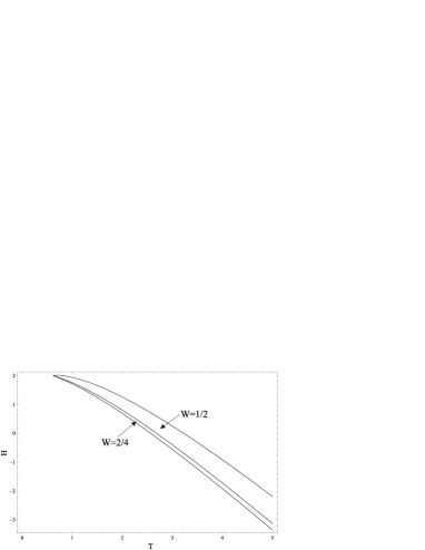
Figure 6: Arnold tongues with winding numbers $\mathrm{w}=1/2$ and $\mathrm{w}=2/4$ for Potts model for $Q=0.8$, $J=-1$, $\gamma=3$.

(a)	(b)

Figure 7: The plot of $M$ (magnetization) versus temperature $T$ for $Q=1.2$, $J=-1$, $\gamma=3$ (a) $H=1.3$; (b) $H=0.2$.

$M$ magnetization can be regarded as a function of $T$, fixing the value of external magnetic field. Fig. 5 indicates, that lowering $H$ first two periodic cycle appears, corresponding to P-2AF1 transition. When the line $H$ intersects the upper curve of the Arnold tongue with $\mathrm{w}=2/4$, one finds a bubble on each branch [Fig. 7(a)]. Here we have P-2AF1-2M2-2AF1 transitions. After the line $H$ intersects the lower curve, we have another two bubbles which points on P-2AF1-2M2-2M3-2M2-2AF1 transitions. With further reduction of external magnetic field new bubbles are formed as parts of the old ones and for still lower $H$’s we reach a region of chaotic behavior [Fig. 7(b)].

6 Three Periodic Window

In this section we will investigate the three periodic window of the Potts-Bethe mapping. Some definite values of parameters $T$ and $H$ form a line in the parameter space, which separates the chaotic and three periodic regimes.

Figure 8: The Plot of $f^{(3)}(x)$ [third iteration of the Potts-Bethe mapping in Eq. (5)] for $Q=1.1$, $J=-1$, $\gamma=3$ at one point of the saddle-node bifurcation line defined by Eq. (36): $T=1.5915$, $H=-1$.

Figure 6 presents the third iteration of the mapping $f(x)$ [Eq. (5)] for one point from that line (as one can see the mapping has three fixed points here). On this line the saddle-node bifurcation takes place, i.e. the aforementioned line can be found from the following condition (see Sec. 5):

$$\left\{\begin{array}[]{ll}f^{(3)}(x)=x&\\ (f^{(3)}(x))^{\prime}=1.&\end{array}\right.$$ (36)

Consequent bifurcations correspond to period doubling, which leads to appearance of stable $3\ast 2^{n}$ periodic cycles. Following the technique described in Sec. 5, we can find the line separating three and six periodic cycles (three and six periodic modulated phases) from the following system of equations:

$$\left\{\begin{array}[]{ll}f^{(3)}(x)=x&\\ (f^{(3)}(x))^{\prime}=-1.&\end{array}\right.$$ (39)

Figure 9: Arnold tongue with winding number $\mathrm{w}=1/3$ for Potts model for $Q=1.1$, $J=-1$, $\gamma=3$ (the insert shows details in the area $H>0$).

(a)	(b)

Figure 10: The plot of $M$ (magnetization) versus temperature $T$ in the three periodic window for $Q=1.1$, $J=-1$, $\gamma=3$ (a) $H=1.3$; (b) $H=1.2$.

Curves found from (36) and (39) form Arnold tongue with winding number $\mathrm{w}=1/3$ (Fig. 6). It corresponds to the area of existence of the three - periodic modulated phase (3M0, i.e. $3\ast 2^{0}=3$ periodic).

One can see from Fig. 6 that in the area $H>0$ the mapping presents interesting behavior. Firstly, when the line $H$ intersects only the upper curve of the Arnold tongue, two edges of the window are plainly distinguishable: the saddle-node bifurcation takes place on both edges and the window is presented with only $3$-periodic cycle [Fig. 10(a)].

Transition between chaotic state and three - periodic modulated phase (3M0) occurs. Secondly when the line $H$ intersects lower line of the Arnold tongue, $3\ast 2^{1}=6$ periodic cycle appears in a form of a bubble, which corresponds to six - periodic modulated phase (3M1, i.e. $3\ast 2^{1}=6$ periodic). This indicates 3M0-3M1 transition. It is obvious that if we continue lowering the values of $H$ new bubbles will appear and ultimately the chaotic region in the window will be reached [Fig. 10(b)]. However, for $H<0$ the saddle-node bifurcation occurs only at one edge of the window. For thorough illustration of the effect, we also present the plots of Lyapunov $\lambda$ exponents in Fig. 11.

We also investigated the behavior of Feigenbaum $\alpha$ and $\delta$ exponents for three periodic window. In comparison with the period doubling, the values of $R_{n}$ will be found from the following condition:

$$f^{(3\ast 2^{n})}_{R_{n}}(x^{*})=x^{*}.$$ (40)

Here again $\alpha$ and $\delta$ converges to the values in Eqs. (10a) and (10b). For example in the case $J=-1$, $T=1$, $\gamma=3$ and $Q=0.8$ for $n=10$, $\delta=4.669160924$ and $\alpha=2.502899839$. For the $const^{\prime}$ in Eq. (11) for the same values of parameters we obtained the following value: $const^{\prime}=-0.0167...$ These results confirm once more the universality hypothesis for rational mapping, which describes $Q$-state Potts model on Bethe lattice.

7 Arnold Tongues
through Feigenbaum
Exponents and Critical
Temperatures

Constructing Arnold tongues for rational mappings like Eq. (5), which describe real statistical systems, is a very complicated and laborious procedure. But it turns out that universality hypothesis (see Sec. 3) is in deep relation with this problem.

(a)	(b)

Figure 11: The plot of the Lyapunov exponent for the Potts-Bethe mapping [Eq. (5)] in the three periodic window versus temperature $T$ for the case $Q=1.1$, $J=-1$, $\gamma=3$ (a) $H=1.3$; (b) $H=1.2$.

It can help in finding a simpler way for constructing Arnold
tongues, knowing only one line in parameter space, on which some $k$th bifurcation takes place. Here $r_{m}$ will be the value of parameter [see Eq. (15)] at $m$th bifurcation point. From the scaling relation for $r_{m}$ and Eq. (18) we can obtain $r_{m}$ in terms of $r_{k}$ ($k\leq m$), $R_{\infty}$ and $\delta$:

$$r_{m}=\frac{\left(r_{k}\delta^{k}-R_{\infty}\delta^{k}+R_{\infty}\delta^{m}\right)}{\delta^{m}}$$ (41)

while $R_{\infty}$ from Eq. (11):

$$R_{\infty}=\frac{\text{$R_{n}$$\delta$}_{n+1}-R_{n}}{\delta-1}.$$ (42)

The convergence of the $R_{\infty}$ to its real value is dependent on the speed of convergence of $\delta$ exponents (for $Q>1$ $n=4$ or $5$ and in the area $Q<1$ $n=5$ or $6$ is enough).

Since $r_{1}$ can be found analytically in contrast with bigger $n$’s, it would be convenient to take $k=1$, and $m>1$ [we already have $r_{1}$, after solving Eq. (23)]:

$$r_{2}=\frac{r_{1}+R_{\infty}\delta-R_{\infty}}{\delta},\hskip 10.0ptfor\hskip 5.0ptm=2,$$ (43a)

$$r_{3}=\frac{R_{\infty}\delta^{2}+r_{1}-R_{\infty}}{\delta^{2}},\hskip 10.0ptfor\hskip 5.0ptm=3.$$ (43b)

For obtaining Arnold tongue analog with winding numbers $\mathrm{w}=1/2$ and $\mathrm{w}=2/4$ we have to find $r_{2}$ and $r_{3}$ for different $T$’s and $H$’s. The problem is that Eq. (8) is true for big $n$’s. However, Eq. (8) remains true if we replace $const$ with $c_{n}$. In this case

$$r_{2}=\frac{\frac{c_{2}\left(r_{1}-R_{\infty}\right)}{c_{1}}+R_{\infty}\delta}{\delta},\hskip 10.0ptfor\hskip 5.0ptm=2,$$ (44a)

$$r_{3}=\frac{R_{\infty}\delta^{2}+\frac{c_{3}\left(r_{1}-R_{\infty}\right)}{c_{1}}}{\delta^{2}},\hskip 10.0ptfor\hskip 5.0ptm=3.$$ (44b)

As one can see, the value of $r_{2}$ and $r_{3}$ from Eqs. (43a) and (43b) are as closer to its real value in Eqs. (44a) and (44b) as closer $\frac{c_{1}}{c_{2}}$ and $\frac{c_{1}}{c_{3}}$ is to $1$. Values of $\frac{c_{1}}{c_{2}}$ e.g. for investigated in the previous section $Q=0.8$ and $Q=1.2$ are $\frac{c_{1}}{c_{2}}=1.46087$ and $\frac{c_{1}}{c_{2}}=1.93921$; $\frac{c_{1}}{c_{3}}=1.48275$ and $\frac{c_{1}}{c_{3}}=2.41653$ respectively (for $T=1$). Hence Eqs. (43a) and (43b) can be regarded as an approximate formula for constructing Arnold tongues.

The faster is convergence of Feigenbaum $\delta$ exponent, the closer $\frac{c_{1}}{c_{2}}$ and $\frac{c_{1}}{c_{3}}$ are to $1$. Hence one can see that there is another reason for investigating the behavior of the Feigenbaum exponents.

We can see from Figs. 5 and 5, that for the cases $Q=1.2$ and $Q=0.8$ there are three critical temperatures $T_{n}$, $T_{c_{1}}$ and $T_{c_{2}}$, at which in absence of external magnetic field transition between different phases takes place:

1. $T_{n}$ is the temperature corresponding to paramagnetic - anti-ferromagnetic phase (P-2AF1) transition (known as Neel temperature). The dependence on $Q$ is shown in Fig. 7(a);

2. $T_{c_{1}}$ is the one corresponding to anti-ferromagnetic - four - periodic modulated phase (2AF1-2M2) transition [Fig. 7(b)];

3. $T_{c_{2}}$, the temperature at which transition between four - periodic and eight - periodic modulated phases (2M2-2M3) occurs (the $Q$ dependence of this temperature qualitatively is the same as of $T_{c_{1}}$).

Investigating the behavior of the Lyapunov exponent we found that critical temperatures $T_{c_{1}}$ and $T_{c_{2}}$ exist not for all $Q$ in the area $1<Q<2$ (the fact that Lyapunov exponent does not become zero indicates the absence of bifurcation, hence the second order phase transition). After $Q=1.5681$ there is no more critical temperature like $T_{c_{1}}$ and after $Q=1.5115$ there is no more critical temperature like $T_{c_{2}}$.

(a)

(b)

Figure 12: The plot of (a) $T_{n}$ (Neel temperature) versus $Q$ for $J=-1$, $\gamma=3$; (b) $T_{c_{1}}$ (critical temperature corresponding to transition between antiferromagnetic and four periodic modulated phases in absence of external magnetic field) versus $Q$ for $J=-1$, $\gamma=3$.

Figure 5 shows that there is some $T_{c}$ (upper bound temperature), below which the system undergoes P-2AF1-P phase transition between paramagnetic and anti-ferromagnetic phases,
which exists only in the area $Q>1$ (e.g. for $Q=1.2$, $J=-1$, $\gamma=3$ $T_{c}=5.2606340$).

8 Conclusion

In this paper we investigated $Q$-state Potts model in an external magnetic field on the Bethe lattice for non-integer $Q$. The model was exactly solved by means of recurrence relation technique and a one-dimensional rational mapping was obtained.

We pointed the relation between phase transition of second order and bifurcation points. The phase structure of the model is investigated by constructing Arnold tongues. For given statistical model they correspond to the area of existence of different phases, i.e. to phase diagrams. We have obtained analogs of Arnold tongues with winding numbers $\mathrm{w}=1/2$ and $\mathrm{w}=2/4$ in period doubling regime. We found the transitions P-2AF1, P-2AF1-2M2-2AF1, P-2AF1-2M2-2M3-2AF1 in the case of fixed $H$ and P-2AF1-P at fixed $T$. The behavior of the mapping describing the system is sensitive to the values of $Q$: case $0<Q<1$ in contrast to $1<Q<2$. We also observed the Lyapunov exponent that describes the large variety of phase transitions that occur in the Potts model. We compared chaotic regions varying temperature and magnetic field and pointed that in the first case it was richer.

We studied the convergence of the Feigenbaum $\alpha$ and $\delta$ exponents for the above mentioned rational mapping for $0<Q<1$ and $1<Q<2$ separately. It was shown that for a real statistical system these exponents coincide with the famous universal ones with high accuracy.

We constructed the Arnold tongue analogs with winding number $\mathrm{w}=1/3$ in the three periodic window and calculated the $\alpha$ and $\delta$ exponents for this area. The obtained values justified the universality hypothesis once more.

We have found an approximate method for constructing Arnold tongues through Feigenbaum exponents, based on universality hypothesis. The main advantage of this kind of approach is the simplicity of numerical calculations in contrast to the rigorous treatment of the problem.

9 Acknowledgement

The authors are grateful to V. V. Hovhannisyan for useful discussions.

This work was partly supported by 1518-PS, PS-1981, PS-2033 ANSEF and ECSP-09-08-sasp NFSAT research grants.

Table 1: Feigenbaum exponents for Potts-Bethe mapping [Eq. (5)] for $T=1$; $J=-1$; $\gamma=3$.

	period
$Q$	doubling	$R_{n}$	$\alpha$	$\delta_{n}$
	$2^{1}=2$	6.148585490…
	$2^{2}=4$	5.624678677…	3.068429829…	5.321086266…
	$2^{3}=8$	5.526220056…	2.580752880…	4.731522199…
	$2^{4}=16$	5.505410977…	2.519238533…	4.688360097…
0.8	$2^{5}=32$	5.500972521…	2.506269470…	4.672585925…
	$2^{6}=64$	5.500022629…	2.503627065…	4.670011847…
	$2^{7}=128$	5.499819226…	2.503059457…	4.669364508…
	$2^{8}=256$	5.499775665…	2.502940259…	4.669237820…
	$......$	……	……	……
	$2^{\infty}=\infty$	5.499764337…
	$2^{1}=2$	3.931868660…
	$2^{2}=4$	2.569022501…	3.358835598…	6.792470680…
	$2^{3}=8$	2.368381788…	2.654374001…	5.057633178…
	$2^{4}=16$	2.328710918…	2.534475897…	4.745030314…
	$2^{5}=32$	2.320350408…	2.509653084…	4.685552342…
1.1	$2^{6}=64$	2.318566091…	2.504352497…	4.672658688…
	$2^{7}=128$	2.318184228…	2.503218367…	4.669946004…
	$2^{8}=256$	2.318102458…	2.502974448…	4.669360473…
	$2^{9}=512$	2.318084946…	2.502922160…	4.669235722…
	$......$	……	……	……
	$2^{\infty}=\infty$	2.318080392…

References

- [1] D. Jeong, H. Hong, B. J. Kim, M. Y. Choi, Phase transition in the Ising model on a small-world network with distance-dependent interactions, Phys. Rev. E68(2) (2003) 027101; M. Keskin, O. Canko, and U. Temizer, Dynamic phase transition in the kinetic spin- Blume-Capel model under a time dependent oscilating external magnetic field, ibid. E72(3) (2005) 036125.
- [2] R. J. Baxter, Exactly Solved Models in Statistical Mechanics (Academic Press, New York, 1982).
- [3] S. R. Broadbent, J. M. Hammersley, Percolation processes, Proc. Cambridge Phil. Soc. 53(03) (1957) 629-641.
- [4] S. B. Santra, Study of finite size effects on directed spiral percolation, Int. J. Mod. Phys. B17(9) (2003) 5555-5564; K. Kieling, T. Rudolph, and J. Eisert, Percolation, renormalization, and quantum computing with non-deterministic gates, Phys. Rev. Lett. 99(13) (2007) 130501.
- [5] X. Qian, Y. Deng, and H. W. J. Blöte, Dilute Potts model in two dimensions, Phys. Rev. E72(5) (2005) 056132.
- [6] C. M. Fortuin and P. W. Kasteleyn, On the random-cluster model. Introduction and relation to other models, Physica 57(4) (1972) 536-564.
- [7] F. Gliozzi, Simulation of Potts models with real and no critical slowing down, Phys. Rev E66(1), 016115 (2002); R. G. Ghulghazaryan, N. S. Ananikian and P. M. A. Sloot, Yang-Lee zeros of the -state Potts model on recursive lattices, ibid. E66(4) (2002) 046110; R.G. Ghulghazaryan and N.S. Ananikian, Partition function zeros of the one-dimensional Potts model: the recursive method, J. Phys. A36(23) (2003) 6297 6312.
- [8] J. L. Jacobsen, J. Salas, and A. D. Sokal, Spanning Forests and the -state Potts Model in the Limit , J. Stat. Phys. 119(5-6) (2005) 1153-1281.
- [9] Y. Deng, T. M. Garoni, and A. D. Sokal, Ferromagnetic phase transition for the Spanning-Forest model ( limit of the Potts model) in three or more dimensions, Phys. Rev. Lett. 98(3) (2007) 030602.
- [10] C. B. Anfinsen, Principles that govern the folding of protein chains, Science 181(96) (1973) 223-230.
- [11] G. Salvi and P. Des Los Rios, Effective interactions cannot replace solvent effects in a lattice model of proteins, Phys. Rev. Lett. 91(25) (2003) 258102.
- [12] T. C. Lubensky and J. Isaacson, Field theory for the statistics of branched polymers, gelation and vulcanizition, Phys. Rev. Lett. 41(12) (1978) 829-832.
- [13] B. Duplantier, Two-dimensional copolymers and exact conformal multifractality, Phys. Rev. Lett. 82(5) (1999) 880-883.
- [14] A. Aharony and P. Pfeuty, Dilute spin glasses at zero temperature and the -state Potts model, J. Phys. C12(3) (1979) L125-L128.
- [15] P. Whittle, Polymer models and generalized Potts-Kasteleyn models, J. Stat. Phys. 75(5-6) (1994) 1063-1092.
- [16] R. H. Swendsen and J.-S. Wang, Non-universal critical dynamics in Monte-Carlo simulation, Phys. Rev. Lett. 58(2) (1987) 86-88; L. Chayes and J. Machta, Graphical representations and cluster algorithms II, Physica A254(3-4) (1998) 477-516.
- [17] G. Ossola and A. D. Sokal, Dynamic critical behavior of the Swendsen-Wang algorithm for the three-dimensional Ising model, Nucl. Phys. B691(3) (2004) 259-291; Y. Deng, T. M. Garoni, J. Machta, G. Ossola, M. Polin, and A. D. Sokal, Critical behavior of the Chayes-Machta-Swendsen-Wang dynamics, Phys. Rev. Lett. 99(5) (2007) 055701.
- [18] N. S. Ananikian, S. K. Dallakian and B. Hu, The chaotic properties of the -state Potts model on the Bethe lattice: , Complex Systems 11 (1997) 213-222; N. S. Ananikian et al., Strange attractors in an antiferromagnetic Ising model, Fractals 5(1) (1997) 175-185;
- [19] P. D. Gujrati, Bethe or Bethe-like lattice calculations are more reliable than conventional mean-field calculations, Phys. Rev. Lett. 74(5) (1995) 809-812.
- [20] J. L. Monroe, Phase diagrams of Ising models on Husimi trees. I. Pure multisite interaction systems, J. Stat. Phys. 65(1-2) (1991) 255-268; N. S. Ananikian and S. K. Dallakian, Multifractal approach to three-site antiferromagnetic Ising model, Physica D107(1) (1997) 75-82.
- [21] T. R. Arakelyan, V. R. Ohanyan, L. N.Ananikyan, N. S. Ananikian, and M. Roger, Multisite-interaction Ising model approach to the solid 3He system on a triangular lattice, Phys. Rev. B67(2) (2003) 024424; L. N. Ananikyan, The Hexagonal Recursive Approximation With Multisite-Interaction Ising Model for the solid and fluid 3He system, Int. J. Mod. Phys. B21(5) (2007) 755-772.
- [22] C. Anteneodo, R. N. P. Maia and R. O. Vallejos, Lyapunov exponent of many-particle systems: testing the stochastic approach, Phys. Rev. E68(3) (2003) 036120; V. Latora, A. Rapisarda, and S. Rufo, Chaotic dynamics and superdiffusion in a Hamiltonian systems with many degrees of freedom, Physica A280(1-2) (2000) 81-86.
- [23] N. S. Ananikian and L. N. Ananikyan, in MATHEMATICAL PHYSICS Proc. of the XI Reg. Conf. Tehran, Iran 2004, eds. S. Rahvar, N. Sadooghi and F. Shojai (World Scientific) (May 2005), pp. 21-26; D. García-Álvarez, A. Stefanovska, and P. V. E. McClintock, High-order synchronization, transitions and competition among Arnold tongues in a rotator under harmonic forcing, Phys. Rev. E77(5) (2008) 056203.
- [24] L. P. Kadanoff, Scaling and Universality in Statistical Physics, Physica A163(1) (1990) 1-14.
- [25] M. J. Feigenbaum, The transition to aperiodic behavior in turbulent systems, Commun. Math. Phys. 77(1) (1980) 65-86.
- [26] M. J. Feigenbaum, Quantitative universality for a class of nonlinear transformations, J. Stat. Phys. 19(1) (1978) 25-52;
- [27] N.S. Ananikian, R. R. Lusiniants, K. A. Oganessyan, The multisite antiferromagnetic Ising spin model and the univeisality of Feingenbaum exponents, JETP Lett. 61(6) (1995) 482-486.
- [28] P. Manneville, Y. Pomeau, Intermittency and the Lorenz model, Phys. Lett. A75(1-2) (1979) 1-2.
- [29] P. Manneville, Y. Pomeau, Different ways to turbulence in dissipative dynamical systems, Physica D1(2) (1980) 219-226.
- [30] H. G. Schuster, Deterministic Chaos (Physic-Verlag, Weinheim, 1984), p. 248.
- [31] J. Marsden, M. McCracken (eds.), The Hopf-Bifurcation and its Applications (Springer-Verlag, New York, 1976).