On hitting times of affine boundaries by reflecting Brownian motion and Bessel processes

Abstract

Firstly, we compute the distribution function for the hitting time of a linear time-dependent boundary $t\mapsto a+bt,\ a\geq 0,\,b\in{\bf R},$ by a reflecting Brownian motion. The main tool hereby is Doob’s formula which gives the probability that Brownian motion started inside a wedge does not hit this wedge. Other key ingredients are the time inversion property of Brownian motion and the time reversal property of diffusion bridges. Secondly, this methodology can also be applied for the three dimensional Bessel process. Thirdly, we consider Bessel bridges from 0 to 0 with dimension parameter $\delta>0$ and show that the probability that such a Bessel bridge crosses an affine boundary is equal to the probability that this Bessel bridge stays below some fixed value.

Keywords: Reflecting Brownian motion, Bessel process, hitting time, linear boundary, time reversal, time inversion, Brownian bridge, Bessel bridge.

AMS Classification: 60J65, 60J60.

1 Introduction

Let $B=\{B_{t}:t\geq 0\}$ denote a real valued Brownian motion and $f:[0,+\infty)\mapsto{\bf R}$ a ”nice” function. Introduce the first hitting time of $f$ by $B$ via

$$H_{f}:=\inf\{t:\,B_{t}=f(t)\}.$$

There are many important applications (e.g. in sequential analysis, see, e.g., Lerche [21], and mathematical finance, especially in the theory of American options, see, e.g., Peskir and Shiryaev [24] Chapter VII) which call for the distribution of $H_{f}$ for some particular functions $f.$ For linear boundaries $f(t)=a+bt$ we refer to Doob [13] and Durbin [14], for square root boundaries $f(t)=\sqrt{a+bt}$ see Breiman [8], Ciffarelli et al. [10], Shepp [33], Delong [11],[12] and Yor [37], and for parabolic boundaries $f(t)=a+bt^{2},$ Groeneboom [19], Salminen [29] and Martin-Löf [22]. We refer to Durbin [15] (with appendix by Williams) for a practical method via integral equations to calculate the hitting probabilities of time dependent boundaries. For the method of images, see Lerche [21]. In Alili and Patie [3] a new approach based on functional transformations of processes is developed and its connection with the method of images is studied.

In this paper we compute the distribution of the hitting time of a linear boundary for

$\bullet$

reflecting Brownian motion (RBM),

$\bullet$

three dimensional Bessel process (BES).

Our approach is based on a formula by Doob presented in [13], as well as the time inversion property for Brownian motion and Bessel processes, and the time reversal property of diffusion bridges. In fact, the case of RBM has been already studied via Doob’s formula and the time inversion by Abundo ([2]; Corollary 3.4) for straight lines with positive slope. For Bessel processes with dimension parameter $\delta>0$ results for hitting times of straight lines through origin can be found in Pitman and Yor ([25]; Section 8 p. 332) and in Alili and Patie ([4]; Theorem 5.1) - we review these results below in Remarks 15 and Theorem 16, respectively.

The above description shows that one of the aims of our paper is to relate formulae about these (classical) first hitting times which appear to be rather scattered in the literature. Moreover, seemingly different formulae for the same densities may be found in different papers but this discrepancy can often be explained, e.g., via the Poisson summation formula.

We now present our main notation. All processes we study are defined on the canonical space $C$ of continuous functions $\omega:{\bf R}_{+}\mapsto{\bf R}.$ Let

$${\cal C}_{t}:=\sigma\{\omega_{s}:=\omega(s):s\leq t\}$$

denote the smallest $\sigma$-algebra making the coordinate mappings up to time $t$ measurable and take ${\cal C}$ to be the smallest $\sigma$-algebra including all $\sigma$-algebras ${\cal C}_{t},\ t\geq 0.$ Processes are identified in $(C,{\cal C})$ via their probability measures; e.g., ${\bf P}^{BM}_{x},$ ${\bf P}^{RBM}_{x},$ and ${\bf P}^{BES(\delta)}_{x}$ denote the probabilities under which the coordinate process with $\omega_{0}=x$ is a Brownian motion, a reflecting Brownian motion and a Bessel process with dimension parameter $\delta$ , respectively.

Throughout the paper the notation

$$H_{a,b}:=\inf\{t\,:\,\omega_{t}=a+bt\}$$

is used for the hitting time of a linear time dependent boundary. Notice that for $x=0$, by the scaling property of Brownian motion and Bessel processes,

$$H_{a,b}\stackrel{{\scriptstyle d}}{{=}}\begin{cases}b^{-2}H_{ab,1},&b>0,\\ b^{-2}H_{a|b|,-1},&b<0,\end{cases}$$ (1)

and if $f_{a,b}$ denotes the density of $H_{a,b}$ then

$$f_{a,b}(u)=\begin{cases}b^{-2}f_{ab,1}(b^{2}u),&b>0,\\ b^{-2}f_{a|b|,-1}(b^{2}u),&b<0.\end{cases}$$ (2)

Also for $x=0,$ the time inversion property - a basic tool in our approach - is valid for Brownian motion and Bessel processes with dimension parameter $\delta>0$ initiated at 0 (for $0<\delta<2$ the Bessel process is assumed to be reflecting at 0), that is, under ${\bf P}^{BM}_{0}$ and ${\bf P}^{BES(\delta)}_{0}$

$$\{\omega_{t}:t>0\}\,\stackrel{{\scriptstyle d}}{{=}}\,\{t\,\omega_{1/t}:t>0\}.$$ (3)

We remark that this property can also be used to derive the distribution of the last hitting time from the distribution of the first hitting time (and vice versa). Indeed, for $a,b>0$ let

$$G_{b,a}:=\sup\{t\,:\,\omega_{t}=b+at\}.$$

Then, under ${\bf P}^{BM}_{0}$ and ${\bf P}^{BES(\delta)}_{0},$ it holds

$$\hskip-28.45274pt\sup\{t\,:\,\omega_{t}=b+at\}\,\stackrel{{\scriptstyle d}}{{=}}\,\sup\{t>0\,:\,t\omega_{1/t}=b+at\}$$

$$\hskip 73.97733pt=\sup\{t\,:\,\omega_{1/t}=\frac{b}{t}+a\}$$

$$\hskip 73.97733pt=1/\inf\{u\,:\,\omega_{u}=a+bu\},$$

and, hence,

$$G_{b,a}\,\stackrel{{\scriptstyle d}}{{=}}\,1/H_{a,b},$$ (4)

in other words, e.g., for $a,b>0$

$${\bf P}^{BES(\delta)}_{0}\left(G_{b,a}<t\right)={\bf P}^{BES(\delta)}_{0}\left(H_{a,b}>\frac{1}{t}\right).$$ (5)

Next we recall well known formulas for the hitting times of constant boundaries by RBM and BES. Firstly,

$${\bf E}^{RBM}_{0}\left(\exp(-\lambda H_{a,0})\right)=\left(\hbox{\rm cosh}(a\sqrt{2\lambda})\right)^{-1}$$ (6)

from which using series expansion and inverting term by term we obtain

$${\bf P}^{RBM}_{0}\left(H_{a,0}\in du\right)/du=\frac{-2a}{\sqrt{2\pi u^{3}}}\sum_{k=-\infty}^{\infty}(4k-1)\,{\rm e}^{-(4k-1)^{2}a^{2}/2u}.$$ (7)

Making an elementary parity manipulation one can find a different but equivalent form for the density of $H_{a,0}$

$${\bf P}^{RBM}_{0}\left(H_{a,0}\in du\right)/du=\frac{a}{\sqrt{2\pi u^{3}}}\sum_{k=-\infty}^{\infty}(-1)^{k}(2k+1)\,{\rm e}^{-(2k+1)^{2}a^{2}/2u}$$ (8)

displayed in [7] p. 355 and 641.

For three dimensional Bessel process it holds

$${\bf E}^{BES(3)}_{0}\left(\exp(-\lambda H_{a,0})\right)=\frac{a\sqrt{2\lambda}}{\hbox{\rm sinh}(a\sqrt{2\lambda})},$$ (9)

and inverting

$${\bf P}^{BES(3)}_{0}\left(H_{a,0}\in du\right)/du$$ (10)

$$\hskip 56.9055pt=\frac{a}{\sqrt{2\pi u^{5}}}\,\sum_{k=-\infty}^{\infty}\left((2k+1)^{2}a^{2}-u\right){\rm e}^{-(2k+1)^{2}a^{2}/2u},$$

which coincides with the formula presented in [7] p. 463 letting therein $x\downarrow 0.$ We refer also to Pitman and Yor [27] where the subordinators, denoted by $C_{t}$ and $S_{t},$ generated by the positive powers of the right hand sides of (6) and (9), respectively, are studied.

For ease of the reader (and of ourselves !), when comparing certain theta function type series indexed by Z or N, we indulge in stating the following elementary lemma.

Lemma 1.

Let $\psi$ be a function defined on odd integers $2k+1,\,k\in{\bf Z}.$ Assume that there exists $\varepsilon$ such that $\psi(2k+1)=\varepsilon\,\psi(-2k-1)$ for all $k\in{\bf Z}.$ Then

$$\sum_{n=-\infty}^{\infty}\psi(2n+1)=(1+\varepsilon)\sum_{k=0}^{\infty}\psi(2k+1),$$

where it is assumed that the sum on the RHS is finite. In particular, if $\psi$ is even, i.e., $\varepsilon=+1$ then

$$\sum_{n=-\infty}^{\infty}\psi(2n+1)=2\sum_{k=0}^{\infty}\psi(2k+1),$$

and if $\psi$ is odd, i.e., $\varepsilon=-1$ then

$$\sum_{n=-\infty}^{\infty}\psi(2n+1)=0.$$

The outline of the paper is as follows: Doob’s formula is discussed in the next section, and in the third section the distribution of $H_{a,b}$ for RBM is presented. In the fourth section the BES case is treated, and the paper concludes with a fifth section, where the distribution of the maximum of a general Bessel bridge is connected with the distribution of $H_{a,b}$ for this Bessel bridge.

2 Doob’s formula

In his famous paper on the Kolmogorov-Smirnov test, Doob [13] derived the expression for the probability that Brownian motion started inside a space-time wedge does not hit this wedge. We first give some symmetry properties of the function characterizing this probability.

Proposition 2.

For $\alpha,\beta,a,b\geq 0$ let

$$\hskip-28.45274ptG(\alpha,\beta;a,b):={\bf P}^{BM}_{0}\left(-(\alpha+\beta t)\leq\omega_{t}\leq a+bt\quad\forall\ t\geq 0\right).$$ (11)

Then $G$ has the symmetry properties

$$G(\alpha,\beta;a,b)=G(\beta,\alpha;b,a)=G(a,b;\alpha,\beta),$$ (12)

and for all $c>0$ the scaling property

$$G(\alpha,\beta;a,b)=G(\frac{\alpha}{c},\beta c;\frac{a}{c},bc).$$ (13)

Proof.

The first equality in (12) follows from time inversion:

$$\hskip-28.45274ptG(\alpha,\beta;a,b)={\bf P}^{BM}_{0}\left(-(\alpha+\beta t)\leq\omega_{t}\leq a+bt\quad\forall\ t>0\right)$$

$$\hskip 31.2982pt={\bf P}^{BM}_{0}\left(-(\alpha+\beta t)\leq t\omega_{1/t}\leq a+bt\quad\forall\ t>0\right)$$

$$\hskip 31.2982pt={\bf P}^{BM}_{0}\left(-(\frac{\alpha}{t}+\beta)\leq\omega_{1/t}\leq\frac{a}{t}+b\quad\forall\ t>0\right)$$

$$\hskip 31.2982pt=G(\beta,\alpha;b,a).$$

The second equality in (12) is obtained by the spatial symmetry of Brownian motion. For (13) consider

$$\hskip-28.45274ptG(\alpha,\beta;a,b)={\bf P}^{BM}_{0}\left(-(\alpha+\beta t)\leq\omega_{t}\leq a+bt\quad\forall\ t>0\right)$$

$$\hskip 31.2982pt={\bf P}^{BM}_{0}\left(-(\alpha+\beta c^{2}t)\leq\omega_{c^{2}t}\leq a+bc^{2}t\quad\forall\ t>0\right)$$

$$\hskip 31.2982pt={\bf P}^{BM}_{0}\left(-(\frac{\alpha}{c}+\beta ct)\leq\frac{1}{c}\,\omega_{c^{2}t}\leq\frac{a}{c}+bct\quad\forall\ t>0\right)$$

$$\hskip 31.2982pt=G(\frac{\alpha}{c},\beta c;\frac{a}{c},bc),$$

where Brownian scaling has been used. ∎

We now state Doob’s formula; for the proof, see [13].

Theorem 3.

For $\alpha,\beta,a,b\geq 0$

$$G(\alpha,\beta;a,b)=1-\sum_{k=1}^{\infty}\left({\rm e}^{-2A_{k}}+{\rm e}^{-2B_{k}}-{\rm e}^{-2C_{k}}-{\rm e}^{-2D_{k}}\right),$$ (14)

where

$$A_{k}:=A_{k}(\alpha,\beta;a,b):=k^{2}ba+(k-1)^{2}\beta\alpha+k(k-1)(b\alpha+a\beta),$$

$$B_{k}:=B_{k}(\alpha,\beta;a,b):=(k-1)^{2}ba+k^{2}\beta\alpha+k(k-1)(b\alpha+a\beta),$$

$$C_{k}:=C_{k}(\alpha,\beta;a,b):=k^{2}(ba+\beta\alpha)+k(k-1)b\alpha+k(k+1)a\beta,$$

$$D_{k}:=D_{k}(\alpha,\beta;a,b):=k^{2}(ba+\beta\alpha)+k(k+1)b\alpha+k(k-1)a\beta.$$

Remark 4.

The symmetry properties of $G$ can, of course, be seen also from the expressions for $A_{k},B_{k},C_{k},$ and $D_{k}.$ Indeed,

$$A_{k}(\alpha,\beta;a,b)=B_{k}(a,b;\alpha,\beta),$$

and, since,

$$C_{k}(\alpha,\beta;a,b)=k^{2}(ba+\beta\alpha)+k^{2}(b\alpha+a\beta)+k(a\beta-b\alpha)$$

and

$$D_{k}(\alpha,\beta;a,b)=k^{2}(ba+\beta\alpha)+k^{2}(b\alpha+a\beta)-k(a\beta-b\alpha),$$

it is easily seen also that

$$C_{k}(\alpha,\beta;a,b)=D_{k}(a,b;\alpha,\beta).$$

Moreover,

$$A_{k}(\alpha,\beta;a,b)=A_{k}(\beta,\alpha;b,a),\ B_{k}(\alpha,\beta;a,b)=B_{k}(\beta,\alpha;b,a)$$

and

$$C_{k}(\alpha,\beta;a,b)=C_{k}(\beta,\alpha;b,a),D_{k}(\alpha,\beta;a,b)=D_{k}(\beta,\alpha;b,a).$$

We also note that each of $A_{k},B_{k},C_{k}$ and $D_{k}$ satisfies the same scaling property as $G.$ Notice also that if we introduce

$$\Upsilon(m,n):=m^{2}ba+n^{2}\beta\alpha+mn(b\alpha+a\beta)$$

then

$$A_{k}=\Upsilon(k,k-1)\quad{\sl and}\quad B_{k}=\Upsilon(k-1,k).$$

The limiting distribution function (found by Kolmogorov) of the Kolmogorov-Smirnov statistics is

$$F_{K}(\lambda):=1+2\sum_{k=1}^{\infty}(-1)^{k}\,{\rm e}^{-2k^{2}\lambda^{2}},\ \lambda>0,$$

and was identified by Doob to be the distribution function of the maximum of the absolute value of a standard Brownian bridge. Moreover, Doob observed that this distribution function is closely related to the probability that RBM never hits a straight line with positive slope. Indeed, taking in (11) $\alpha=a$ and $\beta=b$ gives

$$A_{k}=B_{k}=(2k-1)^{2}ba\quad{\rm and}\quad C_{k}=D_{k}=(2k)^{2}ba,$$

and yields this probability as displayed in the following

Corollary 5.

For $a,b\geq 0$ it holds

$$\hskip-42.67912pt{\bf P}^{BM}_{0}\left(|\omega_{t}|\leq a+bt\quad\forall\ t\geq 0\right)={\bf P}^{RBM}_{0}\left(H_{a,b}=\infty\right)$$

$$\hskip 99.58464pt=1+2\sum_{k=1}^{\infty}(-1)^{k}\,{\rm e}^{-2k^{2}ab}$$ (15)

$$\hskip 99.58464pt=\Theta^{*}(2ab/\pi),$$

where

$$\Theta^{*}(u):=\sum_{k\in{\bf Z}}(-1)^{k}\,{\rm e}^{-\pi k^{2}u}$$

is the ”modified” Jacobi theta function.

Remark 6.

Trivially, the LHS of (5) equals

$${\bf P}^{BM}_{0}\left(\sup_{t\geq 0}(|\omega_{t}|-bt)\leq a\right)$$

so that $a\mapsto\Theta^{*}(2a^{2}/\pi)$ appears as a distribution function and equals $F_{K}.$ For a more general discussion for such suprema involving Bessel processes, see Theorem 19. We note that the scaling property of Brownian motion also yields that the LHS of (5) is a function of the product $ab$ only.

Using time inversion Abundo [2] (see also Scheike [32]) computed the probability that a Brownian bridge stays inside a space-time wedge. Let $x,y\in{\bf R}$ and $u>0$ be given, and denote by ${\bf P}^{BM}_{x,u,y}$ the probability measure associated with Brownian bridge from $x$ to $y$ of length $u.$ The next result is given in [2], Proposition 3.5 and Theorem 3.3. To make the exposition more self contained we give here a proof which differs slightly from the proof in [2].

Theorem 7.

For $u>0$ and $\alpha,\beta,a,b\geq 0$

$$\hskip-28.45274pt{\bf P}^{BM}_{0,u,y}\left(-(\alpha+\beta t)\leq\omega_{t}\leq a+bt\quad\forall\ t\in(0,u)\right)$$

$$\hskip 56.9055pt=G\left(\alpha,\beta+\frac{\alpha+y}{u};a,b+\frac{a-y}{u}\right),$$ (16)

where $-(\alpha+\beta u)\leq y\leq a+bu$ and $G$ is as defined in (14). In particular, for $\alpha=a,$ $\beta=b,$ and $|y|\leq a+bu$

$$\hskip-28.45274pt{\bf P}^{BM}_{0,u,y}\left(|\omega_{t}|\leq a+bt\quad\forall\ t\in(0,u)\right)$$

$$\hskip 56.9055pt=\sum_{n=-\infty}^{\infty}(-1)^{n}\,\exp\left(-2n^{2}a(b+\frac{a}{u})+2na\frac{y}{u}\right).$$ (17)

Proof.

Using

$$\left(\{\omega_{t};0\leq t\leq u\},{\bf P}^{BM}_{0,u,y}\right)\stackrel{{\scriptstyle d}}{{=}}\left(\{\omega_{t}+\frac{y}{u}t;0\leq t\leq u\},{\bf P}^{BM}_{0,u,0}\right)$$

we write

$$\hskip-14.22636pt{\bf P}^{BM}_{0,u,y}\left(-\alpha-\beta t\leq\omega_{t}\leq a+bt\quad\forall\ t\in(0,u)\right)$$

$$\hskip 28.45274pt={\bf P}^{BM}_{0,u,0}\left(-\alpha-\beta t\leq\omega_{t}+\frac{y}{u}t\leq a+bt\quad\forall\ t\in(0,u)\right)$$

$$\hskip 28.45274pt={\bf P}^{BM}_{0,u,0}\left(-\alpha-(\beta+\frac{y}{u})t\leq\omega_{t}\leq a+(b-\frac{y}{u})t\quad\forall\ t\in(0,u)\right).$$

To proceed recall

$$\left(\{\omega_{t};0\leq t<u\},{\bf P}^{BM}_{0,u,0}\right)\stackrel{{\scriptstyle d}}{{=}}\left(\left\{\frac{u-t}{u}\,\omega_{ut/(u-t)};0\leq t<u\right\},{\bf P}^{BM}_{0}\right)$$

and, hence,

$$\hskip-14.22636pt{\bf P}^{BM}_{0,u,0}\left(-\alpha-(\beta+\frac{y}{u})t\leq\omega_{t}\leq a+(b-\frac{y}{u})t\quad\forall\ t\in(0,u)\right)$$

$$\hskip 28.45274pt={\bf P}^{BM}_{0}\left(-\alpha-(\beta+\frac{y}{u})t\leq\frac{u-t}{u}\,\omega_{ut/(u-t)}\leq a+(b-\frac{y}{u})t\quad\forall\ t\in(0,u)\right)$$

$$\hskip 28.45274pt={\bf P}^{BM}_{0}\left(-\alpha-(\beta+\frac{y}{u})\frac{vu}{v+u}\leq\frac{u}{v+u}\,\omega_{v}\leq a+(b-\frac{y}{u})\frac{vu}{v+u}\quad\forall\ v\geq 0\right)$$

$$\hskip 28.45274pt={\bf P}^{BM}_{0}\left(-\alpha-(\alpha+\beta u+y)\frac{v}{u}\leq\omega_{v}\leq a+(a+bu-y)\frac{v}{u}\quad\forall\ v\geq 0\right)$$

$$\hskip 28.45274pt=G\left(\alpha,\beta+\frac{\alpha+y}{u};a,b+\frac{a-y}{u}\right).$$

by the symmetry property of $G.$ This proves formula (7) and (7) follows immediately. ∎

From (7), integrating over $y$ leads to the distribution function of $H_{a,b},\,a,b\geq 0,$ for RBM, see Abundo [2] Corollary 3.4. In the next section, see Theorem 9, we find this distribution also for negative values of $b.$

Remark 8.

The fact that variables $a,b,y$ and $u$ appear on the RHS of (7) in such a particular way can be explained again (cf. the last sentence in Remark 6) via the scaling property. Indeed, from the proof above (consider the case $u=1$)

$$\hskip-14.22636pt{\bf P}^{BM}_{0,1,y}\left(|\omega_{t}|\leq a+bt\quad\forall\ t\in(0,1)\right)$$

$$\hskip 28.45274pt={\bf P}^{BM}_{0}\left(-a-(a+b+y)v\leq\omega_{v}\leq a+(a+b-y)v\quad\forall\ v\geq 0\right)$$

$$\hskip 28.45274pt={\bf P}^{BM}_{0}\left(-a-(a+b+y)v\leq c\,\omega_{v/c^{2}}\leq a+(a+b-y)v\quad\forall\ v\geq 0\right)$$

$$\hskip 28.45274pt={\bf P}^{BM}_{0}\left(-\frac{a}{c}-(a+b+y)cs\leq\omega_{s}\leq\frac{a}{c}+(a+b-y)cs\quad\forall\ s\geq 0\right).$$

Choosing $c=a$ yields

$$\hskip-28.45274pt{\bf P}^{BM}_{0,1,y}\left(|\omega_{t}|\leq a+bt\quad\forall\ t\in(0,1)\right)$$

$$\hskip 28.45274pt={\bf P}^{BM}_{0}\left(|\omega_{s}+ays|\leq 1+a(a+b)s\quad\forall\ s\geq 0\right)$$

showing that the LHS of (7) can be viewed as a function of $b^{\prime}:=a(a+b)$ and $\mu:=ay$ only.

3 Distribution of $H_{a,b}$ for a reflecting Brownian motion

In the next theorem we give an explicit form of the distribution function of $H_{a,b},\,a>0,b\in{\bf R},$ for RBM initiated at 0. For $b>0$ formula (9) can be found in Abundo [2] Corollary 3.4 (however, there seems to be a misprint in formula (3.6) in [2]; in the exponential $n$ should be replaced by $n^{2}$). Clearly, if RBM is initiated from above the line then the distribution of $H_{a,b}$ can be obtained from the distribution of $H_{a,b}$ for BM.

Theorem 9.

For $a>0$ and $b\in{\bf R}$ and $u>0$ such that $u<-(a/b)$ for $b<0$ and there is no constraint if $b>0$ it holds

$$\hskip-28.45274pt{\bf P}^{RBM}_{0}\left(H_{a,b}>u\right)$$

$$\hskip-25.6073pt=\sum_{k=-\infty}^{\infty}(-1)^{k}\hbox{\rm e}^{-2k^{2}ab}\,\left(\Phi\left(\frac{a+bu-2ka}{\sqrt{u}}\right)-\Phi\left(-\frac{a+bu-2ka}{\sqrt{u}}\right)\right),$$ (18)

where $\Phi$ denotes the standard normal distribution function, i.e.,

$$\Phi(x):=\int_{-\infty}^{x}\frac{1}{\sqrt{2\pi}}\,\hbox{\rm e}^{-y^{2}/2}dy.$$ (19)

The density, with the same constraints, is given by

$$\hskip-22.76228pt{\bf P}^{RBM}_{0}\left(H_{a,b}\in du\right)/du$$

$$\hskip-14.22636pt=\frac{1}{\sqrt{2\pi u^{3}}}\sum_{k=-\infty}^{+\infty}(-1)^{k}(a-bu-2ka)\,{\rm e}^{-2k^{2}ab}\,{\rm e}^{-\left(a+bu-2ka\right)^{2}/2u}$$

$$\hskip-14.22636pt=:\Delta_{a,b}(u).$$ (20)

Moreover, in case $b>0$

$${\bf P}^{RBM}_{0}\left(\omega_{H_{a,b}}>y\right)=\begin{cases}{\bf P}^{RBM}_{0}\left(H_{a,b}>\frac{y-a}{b}\right),&\text{if $y>a$,}\\ 1,&\text{if $y\leq a$,}\end{cases}$$ (21)

and for $y>a$

$${\bf P}^{RBM}_{0}\left(\omega_{H_{a,b}}\in dy\right)/dy=\frac{1}{b}\Delta_{a,b}(\frac{y-a}{b});$$ (22)

in case $b<0$

$${\bf P}^{RBM}_{0}\left(\omega_{H_{a,b}}<y\right)=\begin{cases}{\bf P}^{RBM}_{0}\left(H_{a,b}>\frac{y-a}{b}\right),&\text{if $y<a$,}\\ 1,&\text{if $y\geq a$,}\end{cases}$$ (23)

and for $y<a$

$${\bf P}^{RBM}_{0}\left(\omega_{H_{a,b}}\in dy\right)/dy=\frac{1}{|b|}\Delta_{a,b}(\frac{y-a}{b}).$$ (24)

Proof.

We need to prove the result for $b<0$ (for $b>0$ see [2]). For this, by scaling, it is enough to consider $H_{a,-1},$ i.e., we take $b=-1$ (cf. (1)). Using formula (7) in Theorem 7 we have for $u<a$

$$\hskip-19.91684pt{\bf P}^{RBM}_{0}\left(H_{a,-1}>u\right)=\int_{0}^{a-u}{\bf P}^{RBM}_{0}\left(H_{a,-1}>u\,,\,\omega_{u}\in dy\right)$$

$$\hskip 48.36958pt=\int_{0}^{a-u}{\bf P}^{RBM}_{0}\left(H_{a,-1}>u\,|\,\omega_{u}=y\right)\,{\bf P}^{RBM}_{0}(\omega_{u}\in dy)$$

$$\hskip 48.36958pt=\int_{-(a-u)}^{a-u}{\bf P}^{BM}_{0,u,y}\left(-(a-s)<\omega_{s}<a-s\ \ \forall s\in(0,u)\right)$$

$$\hskip 184.9429pt\times\,{\bf P}^{BM}_{0}(\omega_{u}\in dy)$$

$$\hskip 48.36958pt=\int_{-(a-u)}^{a-u}{\bf P}^{BM}_{y,u,0}\left(-(s-(u-a))<\omega_{s}<s-(u-a)\ \ \forall s\in(0,u)\right)$$

$$\hskip 184.9429pt\times\,{\bf P}^{BM}_{0}(\omega_{u}\in dy),$$ (25)

where, in the last step, we have used the time reversal property of diffusion bridges, see Salminen [30], i.e., for Brownian bridge we have

$$\left(\{\omega_{t}:0\leq t\leq u\},{\bf P}^{BM}_{x,u,y}\right)\stackrel{{\scriptstyle d}}{{=}}\left(\{\omega_{u-t}:0\leq t\leq u\},{\bf P}^{BM}_{y,u,x}\right).$$ (26)

Using spatial homogeneity and (7) in Theorem 7 we obtain

$${\bf P}^{BM}_{y,u,0}\left(-(s-(u-a))<\omega_{s}<s-(u-a)\ \ \forall s\in(0,u)\right)$$

$$\hskip 14.22636pt={\bf P}^{BM}_{0,u,-y}\left(-(s-(u-a))-y<\omega_{s}<s-(u-a)-y\ \ \forall s\in(0,u)\right).$$

$$\hskip 14.22636pt={\bf P}^{BM}_{0,u,-y}\left(-(a-u+y+s)<\omega_{s}<a-u-y+s\ \ \forall s\in(0,u)\right).$$

$$\hskip 14.22636pt=G(a-u+y,\frac{a}{u};a-u-y,\frac{a}{u}).$$

To write down the explicit form of the function $G$ we use (14), and to stress the dependence of $A_{k},$ $B_{k},$ $C_{k},$ and $D_{k}$ on $y$ we use notations $A_{k}(y),$ $B_{k}(y),$ $C_{k}(y),$ and $D_{k}(y),$ respectively. It holds

$$A_{k}(y)=\frac{a}{u}\left(k^{2}(a-u-y)+(k-1)^{2}(a-u+y)+2k(k-1)(a-u)\right)$$

$$\hskip 31.2982pt=-(2k-1)^{2}a+\frac{1}{u}\left((2k-1)^{2}a^{2}-(2k-1)ay\right),$$

$$B_{k}(y)=\frac{a}{u}\left((k-1)^{2}(a-u-y)+k^{2}(a-u+y)+2k(k-1)(a-u)\right)$$

$$\hskip 31.2982pt=-(2k-1)^{2}a+\frac{1}{u}\left((2k-1)^{2}a^{2}+(2k-1)ay\right),$$

$$C_{k}(y)=\frac{a}{u}\left(2k^{2}(a-u)+k(k-1)(a-u-y)+k(k+1)(a-u+y)\right)$$

$$\hskip 31.2982pt=-(2k)^{2}a+\frac{1}{u}\left((2k)^{2}a^{2}+2kay\right),$$

and

$$D_{k}(y)=\frac{a}{u}\left(2k^{2}(a-u)+k(k+1)(a-u-y)+k(k-1)(a-u+y)\right)$$

$$\hskip 32.72049pt=-(2k)^{2}a+\frac{1}{u}\left((2k)^{2}a^{2}-2kay\right).$$

Now we have, see (3),

$$\hskip-22.76228pt{\bf P}^{RBM}_{0}\left(H_{a,-1}>u\right)$$ (27)

$$\hskip-25.6073pt=\int_{-(a-u)}^{a-u}\left(1-\sum_{k=1}^{\infty}\left({\rm e}^{-2A_{k}(y)}+{\rm e}^{-2B_{k}(y)}-{\rm e}^{-2C_{k}(y)}-{\rm e}^{-2D_{k}(y)}\right)\right)\,\varphi_{u}(y)\,dy,$$

where

$$\varphi_{u}(y):=\frac{1}{\sqrt{2\pi u}}\,\hbox{\rm e}^{-y^{2}/2u}.$$

Straightforward integration yields:

$$\hskip-14.22636pt\int_{-(a-u)}^{a-u}{\rm e}^{-2A_{k}(y)}\,\varphi_{u}(y)\,dy$$

$$=\int_{-(a-u)}^{a-u}\,\frac{1}{\sqrt{2\pi u}}\,\exp\left(-\frac{y^{2}}{2u}-\frac{2}{u}\left((2k-1)^{2}a^{2}-(2k-1)ay\right)\right)\,dy$$

$$=\hbox{\rm e}^{2(2k-1)^{2}a}\int_{-(a-u)}^{a-u}\,\frac{1}{\sqrt{2\pi u}}\,\hbox{\rm e}^{-\left(y-2(2k-1)a\right)^{2}/2u}\,dy$$

$$=\hbox{\rm e}^{2(2k-1)^{2}a}\left(\Phi\left(\frac{a-u-2(2k-1)a}{\sqrt{u}}\right)-\Phi\left(\frac{-(a-u)-2(2k-1)a}{\sqrt{u}}\right)\right)$$

$$=:{\bf A}(k,u),$$

$$\hskip-14.22636pt\int_{-(a-u)}^{a-u}{\rm e}^{-2B_{k}(y)}\,\varphi_{u}(y)\,dy$$

$$=\hbox{\rm e}^{2(2k-1)^{2}a}\left(\Phi\left(\frac{a-u+2(2k-1)a}{\sqrt{u}}\right)-\Phi\left(\frac{-(a-u)+2(2k-1)a}{\sqrt{u}}\right)\right)$$

$$=:{\bf B}(k,u),$$

$$\hskip-51.21504pt\int_{-(a-u)}^{a-u}{\rm e}^{-2C_{k}(y)}\,\varphi_{u}(y)\,dy$$

$$=\hbox{\rm e}^{2(2k)^{2}a}\left(\Phi\left(\frac{a-u+4ka}{\sqrt{u}}\right)-\Phi\left(\frac{-(a-u)+4ka}{\sqrt{u}}\right)\right)$$

$$=:{\bf C}(k,u),$$

and

$$\hskip-51.21504pt\int_{-(a-u)}^{a-u}{\rm e}^{-2D_{k}(y)}\,\varphi_{u}(y)\,dy$$

$$=\hbox{\rm e}^{2(2k)^{2}a}\left(\Phi\left(\frac{a-u-4ka}{\sqrt{u}}\right)-\Phi\left(\frac{-(a-u)-4ka}{\sqrt{u}}\right)\right)$$

$$=:{\bf D}(k,u).$$

Hence, we have

$$\hskip-28.45274pt{\bf P}_{0}^{RBM}\left(H_{a,-1}>u\right)$$ (28)

$$\hskip 14.22636pt={\bf I}(0,u)-\sum_{k=1}^{\infty}\left({\bf A}(k,u)+{\bf B}(k,u)-{\bf C}(k,u)-{\bf D}(k,u)\right),$$

where

$${\bf I}(0,u)=\Phi\left(\frac{a-u}{\sqrt{u}}\right)-\Phi\left(-\frac{a-u}{\sqrt{u}}\right).$$

Rearranging the terms in (28) yields (9) with $b=-1,$ and differentiating term by term leads to the density given in (9). ∎

Remark 10.

Taking in (9) $b=0$ and differentiating yields formula (8) for the density of the hitting time of a point for RBM. Clearly, the density given in (9) also converges as $b\to 0$ to (8).

4 Distribution of $H_{a,b}$ for a 3-dimensional Bessel process

In this section we derive an expression for the distribution function of $H_{a,b}$ for a 3-dimensional Bessel process initiated at 0. The probability measures associated with a Bessel bridge from $x$ to $y$ of length $u$ with dimension parameter 3 and a killed (at 0) Brownian bridge are denoted by ${\bf P}^{BES}_{x,u,y}$ and ${\bf P}^{KBM}_{x,u,y},$ respectively. Recall that, in fact,

$${\bf P}^{KBM}_{x,u,y}={\bf P}^{BES}_{x,u,y}$$ (29)

which follows from BES being Doob’s $h$-transform of KBM with $h(x)=x,$ i.e., for $\Gamma_{t}\in{\cal C}_{t}$ and $y>0$

$${\bf P}^{BES}_{y}(\Gamma_{t})={\bf E}^{BM}_{y}\left(\frac{\omega_{t\wedge H_{0}}}{y}\,;\,\Gamma_{t}\right)$$ (30)

(see McKean [23], Williams [36], Revuz and Yor [28] p. 450 and Borodin and Salminen [7] p. 75). However, for some arguments below it is good to have a different notation since these bridges are conditioned from different processes.

We start with a proposition which says that a Brownian bridge from $x>0$ to $y>0$ conditioned not to hit 0 is identical in law with the killed Brownian bridge.

Proposition 11.

For $x,y,u>0$

$${\bf P}^{KBM}_{x,u,y}={\bf P}^{BM}_{x,u,y}\left(\,\cdot\ |\ \omega_{t}>0\quad\forall\,0\leq t\leq u\right).$$ (31)

Proof.

For $0<u_{1}<\dots<u_{n}<u$ consider

$$\hskip-22.76228pt{\bf P}^{BM}_{x,u,y}\left(\omega_{u_{1}}\in dz_{1},\dots,\omega_{u_{n}}\in dz_{n}\,;\,\omega_{t}>0\quad\forall\ 0\leq t\leq u\right)$$

$$\hskip-5.69046pt={\bf P}^{BM}_{x}\left(\omega_{u_{1}}\in dz_{1},\dots,\omega_{u_{n}}\in dz_{n},\omega_{u}\in dy\,;\,H_{0}>u\right)/{\bf P}^{BM}_{x}\left(\omega_{u}\in dy\right)$$

$$\hskip-5.69046pt={\bf P}^{KBM}_{x}\left(\omega_{u_{1}}\in dz_{1},\dots,\omega_{u_{n}}\in dz_{n},\omega_{u}\in dy\right)/{\bf P}^{BM}_{x}\left(\omega_{u}\in dy\right),$$

where $H_{0}:=\inf\{t:\omega_{t}=0\}.$ Similarly,

$${\bf P}^{BM}_{x,u,y}\left(\omega_{t}>0\quad\forall\ 0\leq t\leq u\right)={\bf P}^{KBM}_{x}\left(\omega_{u}\in dy\right)/{\bf P}^{BM}_{x}\left(\omega_{u}\in dy\right).$$

Consequently,

$$\hskip-22.76228pt{\bf P}^{BM}_{x,u,y}\left(\omega_{u_{1}}\in dz_{1},\dots,\omega_{u_{n}}\in dz_{n}\,|\,\omega_{t}>0\quad\forall\ 0\leq t\leq u\right)$$

$$\hskip-5.69046pt={\bf P}^{KBM}_{x}\left(\omega_{u_{1}}\in dz_{1},\dots,\omega_{u_{n}}\in dz_{n},\omega_{u}\in dy\right)/{\bf P}^{KBM}_{x}\left(\omega_{u}\in dy\right)$$

$$\hskip-5.69046pt={\bf P}^{KBM}_{x,u,y}\left(\omega_{u_{1}}\in dz_{1},\dots,\omega_{u_{n}}\in dz_{n}\right).$$

Then, the monotone class theorem implies the stated identity. ∎

Theorem 12.

For $a>0$ and $b\in{\bf R}$ such that $u<-(a/b)$ for $b<0$ (and there is no constraint if $b>0$) it holds

$${\bf P}^{BES}_{0}\left(H_{a,b}>u\right)$$

$$\hskip 28.45274pt=2\sum_{k=-\infty}^{\infty}\hbox{\rm e}^{-2k^{2}ab}\,\Big{[}\left(1-4k^{2}ab\right)\left(\Phi\left(\frac{a+bu-2ka}{\sqrt{u}}\right)-\Phi\left(-\frac{2ka}{\sqrt{u}}\right)\right)$$

$$\hskip 56.9055pt-\frac{2kbu-a-bu}{\sqrt{u}}\,\varphi\left(\frac{a+bu-2ka}{\sqrt{u}}\right)\Big{]},$$ (32)

where $\varphi$ is the standard normal density.

Proof.

Consider first the case $b<0$ and $u<-(a/b).$ Without loss of generality we may take $b=-1.$ Proceeding as in the proof of Theorem 9 (cf. (3)) we have

$$\hskip-19.91684pt{\bf P}^{BES}_{0}\left(H_{a,-1}>u\right)=\int_{0}^{a-u}{\bf P}^{BES}_{y,u,0}\left(\omega_{s}<s+a-u\ \forall s\in(0,u)\right)$$

$$\hskip 184.9429pt\times\,{\bf P}^{BES}_{0}(\omega_{u}\in dy).$$ (33)

By (29) and (31),

$$\hskip-19.91684pt{\bf P}^{BES}_{y,u,0}\left(\omega_{s}<s+a-u\ \forall s\in(0,u)\right)$$

$$\hskip 42.67912pt={\bf P}^{KBM}_{y,u,0}\left(\omega_{s}<s+a-u\ \forall s\in(0,u)\right)$$

$$\hskip 42.67912pt=\lim_{x\downarrow 0}\frac{{\bf P}^{BM}_{y,u,x}\left(0<\omega_{s}<s+a-u\ \forall s\in(0,u)\right)}{{\bf P}^{BM}_{y,u,x}\left(\omega_{s}>0\ \forall s\in(0,u)\right)}.$$ (34)

From Theorem 7 formula (7) we have for $x,y>0$

$${\bf P}^{BM}_{y,u,x}\left(0<\omega_{s}<s+a-u\ \forall s\in(0,u)\right)$$

$$\hskip 42.67912pt={\bf P}^{BM}_{0,u,x-y}\left(-y<\omega_{s}<s+a-u-y\ \forall s\in(0,u)\right)$$

$$\hskip 42.67912pt=G\left(y,\frac{x}{u},a-u-y,\frac{a-x}{u}\right),$$ (35)

and

$${\bf P}^{BM}_{y,u,x}\left(\omega_{s}>0\ \forall s\in(0,u)\right)$$

$$\hskip 42.67912pt=\lim_{N\to\infty}{\bf P}^{BM}_{0,u,x-y}\left(-y<\omega_{s}<N-y\ \forall s\in(0,u)\right)$$

$$\hskip 42.67912pt=\lim_{N\to\infty}G\left(y,\frac{x}{u};N-y,\frac{N-x}{u}\right).$$ (36)

From (4) we may recover the well known formula (cf. [7] p. 174)

$${\bf P}^{BM}_{y,u,x}\left(\omega_{s}>0\ \forall s\in(0,u)\right)=1-\hbox{\rm e}^{-2xy/u}.$$ (37)

To write down the explicit form of the function $G$ in (4) we use (14). The functions $A_{k},B_{k},C_{k}$ and $D_{k}$ are now denoted by $A_{k}(x,y),B_{k}(x,y),C_{k}(x,y)$ and $D_{k}(x,y)$ and it holds

$$\hskip-28.45274ptA_{k}(x,y)=\frac{1}{u}\big{[}k^{2}(a-u-y)(a-x)+(k-1)^{2}xy$$

$$\hskip 56.9055pt+k(k-1)((a-u-y)x+(a-x)y)\big{]},$$

$$\hskip-28.45274ptB_{k}(x,y)=\frac{1}{u}\big{[}(k-1)^{2}(a-u-y)(a-x)+k^{2}xy$$

$$\hskip 56.9055pt+k(k-1)\left((a-u-y)x+(a-x)y\right)\big{]},$$

$$\hskip-14.22636ptC_{k}(x,y)=\frac{1}{u}\big{[}k^{2}\left((a-u-y)(a-x)+xy\right)$$

$$\hskip 56.9055pt+k(k-1)(a-u-y)x+k(k+1)(a-x)y\big{]},$$

and

$$\hskip-14.22636ptD_{k}(x,y)=\frac{1}{u}\big{[}k^{2}\left((a-u-y)(a-x)+xy\right)$$

$$\hskip 56.9055pt+k(k+1)(a-u-y)x+k(k-1)(a-x)y\big{]}.$$

Moreover,

$$A_{k}(0,y)=D_{k}(0,y)=\frac{a}{u}\left(k^{2}(a-u)-ky\right),$$

$$B_{k+1}(0,y)=C_{k}(0,y)=\frac{a}{u}\left(k^{2}(a-u)+ky\right),$$

$$A^{\prime}_{k}:=\frac{\partial A_{k}}{\partial x}(x,y)=-k\frac{a-u}{u}+\frac{y}{u},$$

$$B^{\prime}_{k}:=\frac{\partial B_{k}}{\partial x}(x,y)=(k-1)\frac{a-u}{u}+\frac{y}{u},$$

and

$$C^{\prime}_{k}:=\frac{\partial C_{k}}{\partial x}(x,y)=-D^{\prime}_{k}:=-\frac{\partial D_{k}}{\partial x}(x,y)=-k\frac{a-u}{u}.$$

We calculate the limit in (4) using l’Hospital’s rule:

$${\bf P}^{BES}_{y,u,0}\left(\omega_{s}<s+a-u\quad\forall\ s\in(0,u)\right)$$

$$\hskip 28.45274pt=\lim_{x\downarrow 0}\frac{{1-\sum_{k=1}^{\infty}\left({\rm e}^{-2A_{k}}+{\rm e}^{-2B_{k}}-{\rm e}^{-2C_{k}}-{\rm e}^{-2D_{k}}\right)}}{1-\hbox{\rm e}^{-2xy/u}}$$

$$\hskip 28.45274pt=\frac{B^{\prime}_{1}\hbox{\rm e}^{-2B_{1}(0)}+\sum_{k=1}^{\infty}\left(\left(A^{\prime}_{k}-D^{\prime}_{k}\right){\rm e}^{-2A_{k}(0)}+\left(B^{\prime}_{k+1}-C^{\prime}_{k}\right){\rm e}^{-2C_{k}(0)}\right)}{y/u}$$

$$\hskip 28.45274pt=1+\frac{2(a-u)}{y}\,\sum_{k=1}^{\infty}k\,{\rm e}^{2k^{2}a}{\rm e}^{-2k^{2}a^{2}/u}\left({\rm e}^{-2kay/u}-{\rm e}^{2kay/u}\right)$$

$$\hskip 113.81102pt+\sum_{k=1}^{\infty}{\rm e}^{2k^{2}a}{\rm e}^{-2k^{2}a^{2}/u}\left({\rm e}^{-2kay/u}+{\rm e}^{2kay/u}\right)$$

$$\hskip 28.45274pt=\frac{2(a-u)}{y}\,\sum_{k=-\infty}^{\infty}k\,{\rm e}^{2k^{2}a}{\rm e}^{-2k^{2}a^{2}/u}{\rm e}^{-2kay/u}$$

$$\hskip 113.81102pt+\sum_{k=-\infty}^{\infty}{\rm e}^{2k^{2}a}{\rm e}^{-2k^{2}a^{2}/u}{\rm e}^{-2kay/u}$$

$$\hskip 28.45274pt=\sum_{k=-\infty}^{\infty}\left(1-\frac{2k(a-u)}{y}\right){\rm e}^{2k^{2}a}{\rm e}^{-2k^{2}a^{2}/u}{\rm e}^{2kay/u},$$ (38)

where, in the second step, $B_{1}(0):=B_{1}(0,y)=0,A_{k}(0):=A_{k}(0,y),$ and $C_{k}(0):=C_{k}(0,y).$ Now we can proceed by evaluating the integral given in (4). Recall that

$${\bf P}^{BES}_{0}(\omega_{u}\in dy)=\frac{2y^{2}}{\sqrt{2\pi u^{3}}}\,\hbox{\rm e}^{-y^{2}/2u}\,dy,$$

and consider the integrals

$$\hskip-28.45274ptI_{1}:=\int_{0}^{a-u}{\rm e}^{-2k^{2}a^{2}/u}{\rm e}^{2kay/u}\,\frac{2y^{2}}{\sqrt{2\pi u^{3}}}\,\hbox{\rm e}^{-y^{2}/2u}\,dy$$

$$\hskip-14.22636pt=\int_{0}^{a-u}\frac{2y^{2}}{\sqrt{2\pi u^{3}}}\,\hbox{\rm e}^{-(y-2ka)^{2}/2u}\,dy,$$

and

$$I_{2}:=\int_{0}^{a-u}\frac{2k(a-u)}{y}\,{\rm e}^{-2k^{2}a^{2}/u}{\rm e}^{2kay/u}\,\frac{2y^{2}}{\sqrt{2\pi u^{3}}}\,\hbox{\rm e}^{-y^{2}/2u}\,dy$$

$$\hskip 14.22636pt=2k(a-u)\int_{0}^{a-u}\frac{2y}{\sqrt{2\pi u^{3}}}\,\hbox{\rm e}^{-(y-2ka)^{2}/2u}\,dy.$$

Writing

$$\hskip-28.45274ptI_{1}=\int_{0}^{a-u}\frac{2y(y-2ka)}{\sqrt{2\pi u^{3}}}\,\hbox{\rm e}^{-(y-2ka)^{2}/2u}\,dy$$

$$\hskip 56.9055pt+2ka\int_{0}^{a-u}\frac{2y}{\sqrt{2\pi u^{3}}}\,\hbox{\rm e}^{-(y-2ka)^{2}/2u}\,dy$$

$$\hskip-14.22636pt=:I_{11}+I_{12},$$

and

$$\hskip-28.45274ptI_{2}=2ka\int_{0}^{a-u}\frac{2y}{\sqrt{2\pi u^{3}}}\,\hbox{\rm e}^{-(y-2ka)^{2}/2u}\,dy$$

$$\hskip 56.9055pt-2k\int_{0}^{a-u}\frac{2y}{\sqrt{2\pi u}}\,\hbox{\rm e}^{-(y-2ka)^{2}/2u}\,dy$$

$$\hskip-14.22636pt=:I_{21}-I_{22}$$

it is seen that $I_{12}=I_{21}.$ Straightforward calculations yield

$$I_{11}=-2\,\frac{a-u}{\sqrt{u}}\,\varphi\left(\frac{a-u-2ka}{\sqrt{u}}\right)+2\left(\Phi\left(\frac{a-u-2ka}{\sqrt{u}}\right)-\Phi\left(-\frac{2ka}{\sqrt{u}}\right)\right).$$

Furthermore,

$$\hskip-28.45274ptI_{22}=2k\sqrt{u}\,\int_{0}^{a-u}\frac{2(y-2ka)}{\sqrt{2\pi}\,u}\,\hbox{\rm e}^{-(y-2ka)^{2}/2u}\,dy$$

$$\hskip 56.9055pt+2(2k)^{2}a\,\int_{0}^{a-u}\frac{1}{\sqrt{2\pi u}}\,\hbox{\rm e}^{-(y-2ka)^{2}/2u}\,dy$$

$$\hskip-14.22636pt=4k\sqrt{u}\,\left(\varphi\left(\frac{2ka}{\sqrt{u}}\right)-\varphi\left(\frac{a-u-2ka}{\sqrt{u}}\right)\right)$$

$$\hskip 56.9055pt+2(2k)^{2}a\left(\Phi\left(\frac{a-u-2ka}{\sqrt{u}}\right)-\Phi\left(-\frac{2ka}{\sqrt{u}}\right)\right).$$

Consequently,

$$\hskip-28.45274pt{\bf P}^{BES}_{0}\left(H_{a,-1}>u\right)=\sum_{k=-\infty}^{\infty}{\rm e}^{2k^{2}a}\left(I_{1}-I_{2}\right)$$

$$\hskip 61.17325pt=\sum_{k=-\infty}^{\infty}{\rm e}^{2k^{2}a}\left(I_{11}+I_{22}\right)$$

$$\hskip 61.17325pt=2\,\sum_{k=-\infty}^{\infty}{\rm e}^{2k^{2}a}\Big{[}\left(\frac{2ku-a+u}{\sqrt{u}}\right)\varphi\left(\frac{a-u-2ka}{\sqrt{u}}\right)$$

$$\hskip 71.13188pt+\left(1+(2k)^{2}a\right)\left(\Phi\left(\frac{a-u-2ka}{\sqrt{u}}\right)-\Phi\left(-\frac{2ka}{\sqrt{u}}\right)\right)\Big{]},$$

which is the claimed formula for $b=-1,$ and, by scaling (see (1)) we may extend this for general $b<0.$

Let now $b=1,$ and consider

$$\hskip-19.91684pt{\bf P}^{BES}_{0}\left(H_{a,1}>u\right)=\int_{0}^{a+u}{\bf P}^{BES}_{0,u,y}\left(\omega_{s}<s+a\ \forall s\in(0,u)\right)$$

$$\hskip 184.9429pt\times\,{\bf P}^{BES}_{0}(\omega_{u}\in dy).$$ (39)

We have (see (4))

$$\hskip-19.91684pt{\bf P}^{BES}_{0,u,y}\left(\omega_{s}<s+a\ \forall s\in(0,u)\right)$$

$$\hskip 42.67912pt=\lim_{x\downarrow 0}\frac{{\bf P}^{BM}_{x,u,y}\left(0<\omega_{s}<s+a\ \forall s\in(0,u)\right)}{{\bf P}^{BM}_{x,u,y}\left(\omega_{s}>0\ \forall s\in(0,u)\right)}.$$ (40)

Using (7) gives (see (4))

$${\bf P}^{BM}_{x,u,y}\left(0<\omega_{s}<s+a\ \forall s\in(0,u)\right)$$

$$\hskip 56.9055pt={\bf P}^{BM}_{0,u,y-x}\left(-x<\omega_{s}<s+a-x\ \forall s\in(0,u)\right)$$

$$\hskip 56.9055pt=G\left(x,\frac{y}{u};a-x,1+\frac{a-y}{u}\right).$$

To find the explicit form of the function $G,$ let $\hat{A}_{k}(x,y),\hat{B}_{k}(x,y),\hat{C}_{k}(x,y),$ and $\hat{D}_{k}(x,y)$ denote now the terms $A_{k},B_{k},C_{k},$ and $D_{k}$ in (14). It holds

$$\hskip-28.45274pt\hat{A}_{k}(x,y)=\frac{1}{u}\big{[}k^{2}(a+u-y)(a-x)+(k-1)^{2}xy$$

$$\hskip 56.9055pt+k(k-1)((a+u-y)x+(a-x)y)\big{]},$$

$$\hskip-28.45274pt\hat{B}_{k}(x,y)=\frac{1}{u}\big{[}(k-1)^{2}(a+u-y)(a-x)+k^{2}xy$$

$$\hskip 56.9055pt+k(k-1)\left((a+u-y)x+(a-x)y\right)\big{]},$$

$$\hskip-14.22636pt\hat{C}_{k}(x,y)=\frac{1}{u}\big{[}k^{2}\left((a+u-y)(a-x)+xy\right)$$

$$\hskip 56.9055pt+k(k-1)(a-x)y+k(k+1)(a+u-y)x\big{]},$$

and

$$\hskip-14.22636pt\hat{D}_{k}(x,y)=\frac{1}{u}\big{[}k^{2}\left((a+u-y)(a-x)+xy\right)$$

$$\hskip 56.9055pt+k(k+1)(a-x)y+k(k-1)(a+u-y)x\big{]}.$$

Notice that, e.g., $\hat{A}_{k}(x,y)$ can be obtained from $A_{k}(x,y)$ by substituting $-u$ instead of $u$ and multiplying by $-1.$

Moreover,

$$\hat{A}_{k}(0,y)=\hat{C}_{k}(0,y)=\frac{a}{u}\left(k^{2}(a+u)-ky\right),$$

$$\hat{B}_{k+1}(0,y)=\hat{D}_{k}(0,y)=\frac{a}{u}\left(k^{2}(a+u)+ky\right),$$

$$\frac{\partial\hat{A}_{k}}{\partial x}(x,y)=-k\frac{a+u}{u}+\frac{y}{u},$$

$$\frac{\partial B_{k}}{\partial x}=(k-1)\frac{a+u}{u}+\frac{y}{u},$$

and

$$\frac{\partial\hat{C}_{k}}{\partial x}(x,y)=-\frac{\partial\hat{D}_{k}}{\partial x}(x,y)=k\frac{a+u}{u}.$$

Consequently, as in (4),

$${\bf P}^{BES}_{0,u,y}\left(\omega_{t}<a+t\quad\forall\ t\in(0,u)\right)$$

$$\hskip 28.45274pt=1+\frac{2(a+u)}{y}\,\sum_{k=1}^{\infty}k\,{\rm e}^{-2k^{2}a}{\rm e}^{-2k^{2}a^{2}/u}\left({\rm e}^{-2kay/u}-{\rm e}^{2kay/u}\right)$$

$$\hskip 113.81102pt+\sum_{k=1}^{\infty}{\rm e}^{-2k^{2}a}{\rm e}^{-2k^{2}a^{2}/u}\left({\rm e}^{2kay/u}+{\rm e}^{-2kay/u}\right)$$

$$\hskip 28.45274pt=\sum_{k=-\infty}^{\infty}\left(1-\frac{2k(a+u)}{y}\right){\rm e}^{-2k^{2}a}{\rm e}^{-2k^{2}a^{2}/u}{\rm e}^{2kay/u},$$ (41)

and, further,

$$\hskip-28.45274pt{\bf P}^{BES}_{0}\left(H_{a,1}>u\right)=2\,\sum_{k=-\infty}^{\infty}{\rm e}^{-2k^{2}a}\Big{[}\left(\frac{-2ku-a-u}{\sqrt{u}}\right)\varphi\left(\frac{a+u-2ka}{\sqrt{u}}\right)$$

$$\hskip 71.13188pt+\left(1-(2k)^{2}a\right)\left(\Phi\left(\frac{a+u-2ka}{\sqrt{u}}\right)-\Phi\left(-\frac{2ka}{\sqrt{u}}\right)\right)\Big{]}$$

and, by scaling, see (1), we may extend this for general $b\geq 0.$ Since formulas (21)-(24) follow easily, the proof of the theorem is now complete. ∎

Remark 13.

It is easily checked that taking $b=0$ in (12) and differentiating yields formula (10). Moreover, letting $y\downarrow 0$ in (4) and (4), respectively, we obtain the following formula with $b=\pm 1$ (if $b<0$ then the formula is valid for $u<a/(-b)$)

$$\hskip-28.45274pt{\bf P}^{BES}_{0,u,0}\left(\omega_{t}<a+bt\quad\forall\ t\in(0,u)\right)$$

$$\hskip 28.45274pt=1+2\sum_{k=1}^{\infty}\left(1-4k^{2}\frac{a(a+bu)}{u}\right){\rm e}^{-2k^{2}a(a+bu)/u}.$$ (42)

The case with general $b$ can be proved, e.g., via scaling. Notice that this probability is a function of $a(a+bu)/u$ only. In fact, see Theorem 17

$${\bf P}^{BES}_{0,u,0}\left(\omega_{t}<a+bt\quad\forall\ t\in(0,u)\right)={\bf P}^{BES}_{0,1,0}\left(\sup_{t\leq 1}\omega_{t}<\sqrt{\frac{a(a+bu)}{u}}\right)$$

Putting in (13) $b=0$ gives the well known formula for the distribution of the maximum of a Brownian excursion found in Chung [9], see also Kennedy [20], Durrett and Iglehart [16], Biane and Yor [6] and Pitman and Yor [26]. The distribution of the maximum of a general Bessel process is discussed in Theorem 17.

Next we consider the distribution of $H_{a,b}$ for a three dimensional Bessel process initiated above the line $t\mapsto a+bt.$ In this case, the density can be found using (local) absolute continuity of the probability measure induced by the Bessel process with respect to the probability measure induced by a killed Brownian motion.

Theorem 14.

For $x>a>0$ and $b>0$ it holds

$${\bf P}^{BES}_{x}\left(H_{a,b}\in dt\right)=\frac{(a+bt)(x-a)}{tx\sqrt{2\pi t}}{\rm e}^{-(a-x-bt)^{2}/2t}\,dt.$$ (43)

In particular,

$${\bf P}^{BES}_{0}\left(H_{0,b}\in dt\right)=\frac{b}{\sqrt{2\pi t}}{\rm e}^{-b^{2}t/2}\,dt.$$ (44)

Proof.

Since $H_{a,b}<H_{0}$ for $b>0,$ we obtain, using absolute continuity (30),

$${\bf P}^{BES}_{x}\left(H_{a,b}\in dt\right)={\bf E}^{BM}_{x}\left(\frac{\omega_{H_{a,b}}}{x}\,;\,H_{a,b}\in dt\right)$$

$$\hskip 85.35826pt=\frac{a+bt}{x}{\bf P}^{BM}_{x}\left(H_{a,b}\in dt\right)$$

$$\hskip 85.35826pt=\frac{(a+bt)(x-a)}{tx\sqrt{2\pi t}}{\rm e}^{-(a-x-bt)^{2}/2t}\,dt$$

by the well known formula for the density of the hitting time of straight lines for Brownian motion (see, e.g., [7] p. 295). For formula (44), recall that 0 is an entrance boundary point for the three dimensional Bessel process and, hence, (44) is obtained by taking in (43) $a=0$ and letting $x\to 0.$ ∎

Remark 15.

For Bessel processes with dimension parameter $\delta>2$ we have that $H_{0,b}>0$ ${\bf P}^{BES}_{0}$-a.s. for all $b>0$ (see Shiga and Watanabe [34] Theorem 3.3). On the other hand, it is also well known that $\omega_{t}/t\to 0$ ${\bf P}_{x}^{BES(\delta)}$-a.s. for all $x\geq 0.$ Consequently, $0<H_{a,b}<\infty$ a.s. for all $a\geq 0$ and $b>0.$ From Pitman and Yor [25] Section 8 p. 332 the following result for hitting times of lines going through the origin holds

$${\bf P}_{x}^{\delta}\left(H_{0,b}\in dt\right)/dt=(bt)^{\nu}\,{\rm e}^{-\frac{1}{2}\left(b^{2}t+x^{2}/t\right)}/{\left(2tx^{\nu}\,K_{\nu}(xb)\right)},\qquad x>0,$$ (45)

and

$${\bf P}_{0}^{\delta}\left(H_{0,b}\in dt\right)/dt={\left(\dfrac{b^{2}}{2}\right)^{\nu}\,t^{\nu-1}{\rm e}^{-\frac{b^{2}}{2}t}}/{\Gamma(\nu)},$$ (46)

where $\nu=(\delta-2)/2$ and $K_{\nu}$ is the modified Bessel function of the second kind (see Abramowitz and Stegun [1] p. 374). Since $K_{1/2}(x)=\sqrt{\pi}{\rm e}^{-x}/\sqrt{2x}$ and $\Gamma(1/2)=\sqrt{\pi}$ it is seen that formulas (45) and (46) coincide with (43) and (44) in case $\delta=3$ and $a=0.$

Alili and Patie derive in [4] an expression for the density of hitting time of a Bessel process to a straight line. We wish to compare their formulas in case of RBM and BES with the formulas presented in Theorems 9 and 12. The next result is Theorem 5.1 in [4] (we have, however, corrected a misprint in [4] by putting in minus signs in front of $b$ and $b^{2}$ in the exponent of the first exponential).

Theorem 16.

For a Bessel process of dimension parameter $\delta>0$ and initial state $0\leq x\leq a$ it holds

$$\hskip-42.67912pt{\bf P}^{BES(\delta)}_{x}\left(H_{a,b}\in dt\right)/dt=\frac{{\rm e}^{\,-\frac{b}{2a}(a^{2}-x^{2})-\frac{b^{2}}{2}\,t}}{(1+\frac{b}{a}\,t)^{\nu+2}}$$

$$\hskip 56.9055pt\times\sum_{k=1}^{\infty}\frac{x^{-\nu}\,j_{\nu,k}\,J_{\nu}\left(j_{\nu,k}\frac{x}{a}\right)}{a^{2-\nu}\,J_{\nu+1}\left(j_{\nu,k}\right)}\,{\rm e}^{\,-j_{\nu,k}^{2}\frac{t}{2a(a+bt)}},$$ (47)

where $b\in{\bf R},$ $\nu=(\delta-2)/2$ and $J_{\nu}$ is the Bessel function of the first kind and $j_{\nu,k}$ is the ordered sequence of the positive zeros of $J_{\nu}.$ In particular, for RBM starting from 0, i.e., $\nu=-1/2$ and

$$J_{-1/2}(z)=\sqrt{\frac{2}{\pi z}}\,\cos z,\quad J_{1/2}(z)=\sqrt{\frac{2}{\pi z}}\,\sin z,$$

it holds

$$\hskip-28.45274pt{\bf P}^{RBM}_{0}\left(H_{a,b}\in dt\right)/dt=\frac{{\rm e}^{\,-\frac{ba}{2}-\frac{b^{2}t}{2}}}{\sqrt{a}(a+bt)^{3/2}}$$

$$\hskip 56.9055pt\times\sum_{k=1}^{\infty}(-1)^{k+1}(k-\frac{1}{2})\pi\,\exp\left({-((k-\frac{1}{2})\pi)^{2}\,\frac{t}{2a(a+bt)}}\right)$$

$$\hskip 71.13188pt=:D_{a,b}(t).$$ (48)

Comparing the results in Theorems 16 and 9, we obtain, with our notations in (16) and (9), that

$$D_{a,b}(t)=\Delta_{a,b}(t).$$ (49)

This is a Poisson summation type identity to which we would like to devote attention in a forthcoming work [31]. For the moment, we only refer to Feller [18] and Biane, Pitman and Yor [5] for some related discussion.

Figure 1 about here.

Figure 2 about here.

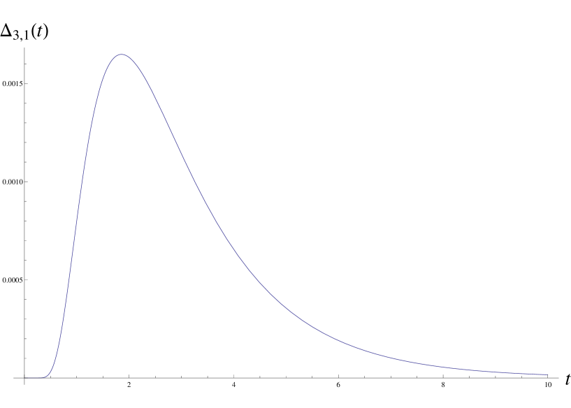
Figure 1: The density of the distribution of the first hitting time of $t\mapsto 3+t$ by RBM started from 0.

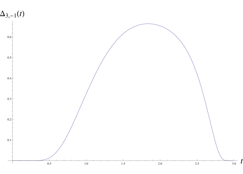
Figure 2: The density of the distribution of the first hitting time of $t\mapsto 3-t$ by RBM started from 0.

5 Results for general Bessel processes

In this section we identify first the probability that a Bessel bridge crosses an affine boundary with the probability that the maximum of the Bessel bridge is below some value. For brevity, we change the notation used above and let ${\bf P}^{(\delta)}_{x}$ denote the probability of a Bessel process with dimension parameter $\delta$ initiated from $x\geq 0.$ Moreover, ${\bf P}^{(\delta)}_{0,u,0}$ denotes the probability measure of a Bessel bridge from 0 to 0 of length $u$. For $0<\delta<2$ the Bessel process is assumed to be instantly reflecting at 0. Secondly, we show that the probability for a Bessel process to stay below the straight line $t\mapsto a+t$ equals to the probability that the maximum of the corresponding Bessel bridge from 0 to 0 of length 1 is less than $\sqrt{a}$.

Theorem 17.

For $a>0,$ $u>0,$ and $b<a/u$

$${\bf P}^{(\delta)}_{0,u,0}\left(\sup_{t\leq u}\{\omega_{t}+bt\}<a\right)={\bf P}^{(\delta)}_{0,u,0}\left(\sup_{t\leq u}\{\omega_{t}\}<\sqrt{a(a-bu)}\right).$$ (50)

Proof.

Consider first the case $b>0$ and let $\Delta_{l}$ denote the left hand side of (50). We have

$$\Delta_{l}={\bf P}^{(\delta)}_{0,u,0}\left(\omega_{t}\leq a-bt\quad\forall 0<t<u\right)$$

$$\hskip 14.22636pt={\bf P}^{(\delta)}_{0,u,0}\left(\omega_{t}\leq a-bu+bt\quad\forall 0<t<u\right)$$

$$\hskip 14.22636pt={\bf P}^{(\delta)}_{0}\left(\omega_{t}\leq a-bu+bt\quad\forall 0<t<u\,|\,\omega_{u}=0\right),$$

where in the second step the time reversal property of diffusion bridges is used (cf. (26)).

By the time inversion of Bessel processes we obtain

$$\Delta_{l}={\bf P}^{(\delta)}_{0}\left(t\,\omega_{1/t}\leq a-bu+bt\quad\forall\ 0<t<u\,|\,u\,\omega_{1/u}=0\right),$$

$$\hskip 14.22636pt={\bf P}^{(\delta)}_{0}\left(\omega_{1/t}\leq(a-bu)\frac{1}{t}+b\quad\forall\ \frac{1}{t}>\frac{1}{u}\,|\,\omega_{1/u}=0\right),$$

$$\hskip 14.22636pt={\bf P}^{(\delta)}_{0}\left(\omega_{s}\leq(a-bu)(s+\frac{1}{u})+b\quad\forall\ s>0\right)$$

$$\hskip 14.22636pt={\bf P}^{(\delta)}_{0}\left(\omega_{s}\leq(a-bu)s+\frac{a}{u}\quad\forall\ s>0\right).$$

Letting $\Delta_{r}$ denote the right hand side of (50) we write

$$\Delta_{r}={\bf P}^{(\delta)}_{0,u,0}0\left(\omega_{t}\leq\sqrt{a(a-bu)}\quad\forall\ 0<t<u\right)$$

$$\hskip 14.22636pt={\bf P}^{(\delta)}_{0}\left(t\,\omega_{1/t}\leq\sqrt{a(a-bu)}\quad\forall\ \frac{1}{t}>\frac{1}{u}\,|\,u\,\omega_{1/u}=0\right)$$

$$\hskip 14.22636pt={\bf P}^{(\delta)}_{0}\left(\omega_{s}\leq\sqrt{a(a-bu)}\,s\quad\forall\ s>\frac{1}{u}\,|\,\omega_{1/u}=0\right)$$

$$\hskip 14.22636pt={\bf P}^{(\delta)}_{0}\left(\omega_{s}\leq\sqrt{a(a-bu)}\left(s+\frac{1}{u}\right)\quad\forall\ s>0\right)$$

$$\hskip 14.22636pt={\bf P}^{(\delta)}_{0}\left(\omega_{s}\leq\sqrt{a(a-bu)}\left(s+\frac{1}{u}\right)\quad\forall\ s>0\right).$$ (51)

Recall that Bessel processes enjoy the Brownian scaling property:

for all $c>0$ under ${\bf P}^{(\delta)}_{0}$

$$\{\sqrt{c}\,\omega_{t/c}:t\geq 0\}\,\stackrel{{\scriptstyle d}}{{=}}\,\{\omega_{t}:t\geq 0\}.$$ (52)

Applying this with $c=(a-bu)/a$ in (5) yields

$$\Delta_{r}={\bf P}^{(\delta)}_{0}\left(\omega_{as/(a-bu)}\leq as+\frac{a}{u}\quad\forall\ s>0\right)$$

$$\hskip 14.22636pt={\bf P}^{(\delta)}_{0}\left(\omega_{t}\leq(a-bu)t+\frac{a}{u}\quad\forall\ t>0\right),$$

which equals $\Delta_{l}.$

For $b<0$ the proof is slightly simpler since we do not use time reversal. Indeed, letting again $\Delta_{l}$ and $\Delta_{r}$ denote the right and left hand side of (50), respectively, we have by time inversion

$$\Delta_{l}={\bf P}^{(\delta)}_{0,u,0}\left(\omega_{t}\leq a-bt\quad\forall\ 0<t<u\right)$$

$$\hskip 14.22636pt={\bf P}^{(\delta)}_{0}\left(\omega_{1/t}\leq\frac{a}{t}-b\quad\forall\ \frac{1}{t}>\frac{1}{u}\,\Big{|}\omega_{1/u}=0\right)$$

$$\hskip 14.22636pt={\bf P}^{(\delta)}_{0}\left(\omega_{s}\leq as+\frac{a-bu}{u}\quad\forall\ s>0\right).$$ (53)

For $\Delta_{r}$ it holds (again) by time inversion

$$\Delta_{r}={\bf P}^{(\delta)}_{0}\left(\omega_{s}\leq\sqrt{a(a-bu)}\left(s+\frac{1}{u}\right)\quad\forall\ s>0\right).$$

Using hereby scaling (52) with $c=a/(a-bu)$ we obtain

$$\Delta_{r}={\bf P}^{(\delta)}_{0}\left(\omega_{(a-bu)s/a}\leq(a-bu)s+\frac{a-bu}{u}\quad\forall\ s>0\right),$$

and substituting $t=(a-bu)s/a$ it is seen that $\Delta_{r}=\Delta_{l},$ thus completing the proof. ∎

Remark 18.

We note that for $b\in{\bf R},$ the result of the theorem may be stated as

$$M_{b}\stackrel{{\scriptstyle d}}{{=}}\sqrt{M^{2}_{0}+\frac{b^{2}}{4}}-\frac{b}{2},$$

where $M_{b}:=\sup_{t\leq 1}\{\omega_{t}-bt\}.$

The next result is a slight extension of Exercise 3.10 in Revuz and Yor [28] where reflecting Brownian motion case is considered. We present here also the proof for the readers’ convenience.

Theorem 19.

For Bessel processes with $\delta>0$ it holds

$${\bf P}^{(\delta)}_{0}\left(\sup_{t\geq 0}\left\{\omega_{t}-t\right\}<a\right)={\bf P}^{(\delta)}_{0,1,0}\left(\sup_{u\leq 1}\left\{\omega_{u}\right\}<\sqrt{a}\right).$$ (54)

In other words, letting $R=\{R_{t}:t\geq 0\}$ denote a Bessel process started from 0 with dimension parameter $\delta>0$ and $R^{0,1,0}=\{R^{0,1,0}_{u}\,:\,0\leq u\leq 1\}$ the corresponding Bessel bridge from 0 to 0 of length 1. Then

$$\sup_{t\geq 0}\left\{R_{t}-t\right\}\,\stackrel{{\scriptstyle d}}{{=}}\,\sup_{u\leq 1}\Big{\{}\left(R^{0,1,0}_{u}\right)^{2}\Big{\}}.$$ (55)

Proof.

Consider for $a>0$

$$\hskip-28.45274pt{\bf P}_{0}\left(\sup_{t\geq 0}\{R_{t}-t\}<a\right)={\bf P}_{0}\left(\forall t,\ R_{t}<a+t\right)$$

$$\hskip 82.51282pt={\bf P}_{0}\left(\forall t,\ R_{\lambda^{2}t}<a+\lambda^{2}t\right)$$

$$\hskip 82.51282pt={\bf P}_{0}\left(\forall t,\ \lambda R_{t}<a+\lambda^{2}t\right)$$

by scaling for any $\lambda>0$. Choosing $\lambda^{2}=a$ yields

$$\hskip-28.45274pt{\bf P}_{0}\left(\sup_{t\geq 0}\{R_{t}-t\}<a\right)={\bf P}_{0}\left(\forall t,\ \sqrt{a}R_{t}<a+at\right)$$

$$\hskip 82.51282pt={\bf P}_{0}\left(\forall t,\ \frac{R_{t}}{1+t}<\sqrt{a}\right),$$

i.e.,

$$\sup_{t\geq 0}\{R_{t}-t\}\,\stackrel{{\scriptstyle d}}{{=}}\,\left(\sup_{t\geq 0}\left\{\frac{R_{t}}{1+t}\right\}\right)^{2}.$$ (56)

We now note that

$$\hskip-21.33955pt\sup_{t\geq 0}\left\{\frac{R_{t}}{1+t}\right\}=\sup_{u\leq 1}\{(1-u)\,R_{u/(1-u)}\}.$$

$$\hskip 56.9055pt\,\stackrel{{\scriptstyle d}}{{=}}\,\sup_{u\leq 1}\{R^{0,1,0}_{u}\},$$ (57)

where, in the first step, we use the substitution $u=t/(1+t),$ and, for the second step, we use the well known representation

$$\{R^{0,1,0}_{u}\,:\,0\leq u<1\}\,\stackrel{{\scriptstyle d}}{{=}}\,\{(1-u)\,R_{u/(1-u)}\,:\,0\leq u<1\},$$

which is inherited from the corresponding Brownian bridge representation. Claim (55) follows now from (56) and (5). ∎

Example 20.

For 3-dimensional Bessel bridge the distribution of the supremum is known. In fact, it was proved by Vervaat [35] that this supremum is identical in law with the range of a standard Brownian bridge, i.e.,

$$\sup_{t\leq u}\Big{\{}R^{0,u,0}_{t}\Big{\}}\,\stackrel{{\scriptstyle d}}{{=}}\,\sup_{t\leq u}B^{0,u,0}_{t}-\inf_{t\leq u}B^{0,u,0}_{t}.$$

The distribution of the range can be deduced from Feller [17], and we have (see [7] p. 174)

$${\bf P}\left(\sup_{t\leq u}B^{0,u,0}_{t}-\inf_{t\leq u}B^{0,u,0}_{t}<y\right)=1+2\sum_{k=1}^{\infty}\left(1-4k^{2}\frac{y^{2}}{u}\right)\,\hbox{\rm e}^{-2k^{2}y^{2}/u}.$$

Consequently, from Theorem 19 for $d=3$

$${\bf P}_{0}(\sup_{t\geq 0}\{R_{t}-t\}<a)=1+2\sum_{k=1}^{\infty}\left(1-4k^{2}a\right)\hbox{\rm e}^{-2k^{2}a}.$$

Example 21.

For 1-dimensional Bessel bridge, i.e., reflecting Brownian bridge, the distribution of the supremum is also known. From [7] p. 333 formula 1.1.8 we obtain

$${\bf P}\left(\sup_{t\leq u}|B^{0,u,0}_{t}|<y\right)=1+2\sum_{k=1}^{\infty}\left(\hbox{\rm e}^{-2(2k)^{2}y^{2}/u}-\hbox{\rm e}^{-2(2k-1)^{2}y^{2}/u}\right)$$

and, hence, from Theorem 19 for $\delta=1$

$${\bf P}_{0}(\sup_{t\geq 0}\{|B_{t}|-t\}<a)=1+2\sum_{k=1}^{\infty}\left(\hbox{\rm e}^{-2(2k)^{2}a}-\hbox{\rm e}^{-2(2k-1)^{2}a}\right)$$

$$\hskip 108.12054pt=1+2\sum_{k=1}^{\infty}(-1)^{k}\hbox{\rm e}^{-2k^{2}a}.$$

This formula may also be obtained from (9) by letting $u\to\infty$ and coincides with (5).

Acknowledgement. We thank Mikhail Stepanov for some numerical computations and creating the plots of $\Delta_{a,b},$ see Figure 1 and 2.

References

[1]
M. Abramowitz and I. Stegun.
Mathematical functions, 9th printing.
Dover publications, Inc., New York, 1970.
[2]
M. Abundo.
Some conditional crossing results of Brownian motion over a
piecewise-linear boundary.
Stat. Probab. Letters, 58:131–145, 2002.
[3]
L. Alili and P. Patie.
On the first crossing times of a Brownian motion and a family of
continuous curves.
C. R. Math. Acad. Sci. Paris, 340(3):225–228, 2005.
[4]
L. Alili and P. Patie.
Boundary crossing identities for diffusions having the time inversion
property.
J. Theor. Probab., 23:65–84, 2010.
[5]
Ph. Biane, J. Pitman, and M. Yor.
Probability laws related to the Jacobi theta and Riemann zeta
functions, and Brownian excursions.
Bull. Amer. Math. Soc. (N.S.), 38(4):435–465 (electronic),
2001.
[6]
Ph. Biane and M. Yor.
Valeurs principales associées aux temps locaux browniens.
Bull. Sci. Math., 111:23–101, 1987.
[7]
A.N. Borodin and P. Salminen.
Handbook of Brownian Motion – Facts and Formulae, 2nd
edition.
Birkhäuser, Basel, Boston, Berlin, 2002.
[8]
L. Breiman.
First exit times from a square root boundary.
In Proc. 5th Berkeley Symp. Math. Stat. Probab. Vol. 2, pages
9–16. University of California, Berkeley, 1967.
[9]
K.L. Chung.
Excursions in Brownian motion.
Arkiv för matematik, 14:155–177, 1976.
[10]
D. M. Cifarelli and E. Regazzini.
Sugli stimatori non distorti a varianza minima di una classe di
funzioni di probabilità troncate.
Giorn. Econom. Ann. Econom. (N.S.), 32:492–501, 1973.
[11]
D. M. DeLong.
Crossing probabilities for a square root boundary by a Bessel
process.
Comm. Statist. A—Theory Methods, 10(21):2197–2213, 1981.
[12]
D.M. DeLong.
Erratum: “Crossing probabilities for a square root boundary by a
Bessel process” [Comm. Statist. A—Theory Methods 10
(1981), no. 21, 2197–2213; MR 82i:62119].
Comm. Statist. A—Theory Methods, 12(14):1699, 1983.
[13]
J.L. Doob.
Heuristic approach to the Kolmogorov-Smirnov theorems.
Ann. Math. Stat., 20:393–403, 1949.
[14]
J. Durbin.
Boundary-crossing probabilities for the Brownian motion and
Poisson processes and techniques for computing the power of the
Kolmogorov-Smirnov test.
J. Appl. Probab., 8:431–453, 1971.
[15]
J. Durbin.
The first passage density of a Brownian motion process to a curved
boundary.
J. Appl. Probab., 29:291–304, 1992.
[16]
R. Durrett and D.I. Iglehart.
Functionals of Brownian meander and Brownian excursion.
Ann. Probab., 5:130–135, 1977.
[17]
W. Feller.
The asymptotic distribution of the range of sums of independent
random variables.
Ann. Math. Stat., 22:427–432, 1951.
[18]
W. Feller.
An introduction to probability theory and its applications.
Vol. II.Second edition. John Wiley & Sons Inc., New York, 1971.
[19]
P. Groeneboom.
Brownian motion with a parabolic drift and Airy functions.
Probab. Theory Related Fields, 81:79–109, 1989.
[20]
D. Kennedy.