1.1in.9in.3in1.4in

Mixture Modeling for Marked Poisson Processes

Matthew A. Taddy
taddy@chicagobooth.edu
The University of Chicago Booth School of Business
5807 South Woodlawn Ave, Chicago, IL 60637, USA

Athanasios Kottas
thanos@ams.ucsc.edu
Department of Applied Mathematics and Statistics
University of California, Santa Cruz
1156 High Street, Santa Cruz, CA 95064, USA

Abstract: We propose a general modeling framework for marked Poisson processes observed over time or space. The modeling approach exploits the connection of the nonhomogeneous Poisson process intensity with a density function. Nonparametric Dirichlet process mixtures for this density, combined with nonparametric or semiparametric modeling for the mark distribution, yield flexible prior models for the marked Poisson process. In particular, we focus on fully nonparametric model formulations that build the mark density and intensity function from a joint nonparametric mixture, and provide guidelines for straightforward application of these techniques. A key feature of such models is that they can yield flexible inference about the conditional distribution for multivariate marks without requiring specification of a complicated dependence scheme. We address issues relating to choice of the Dirichlet process mixture kernels, and develop methods for prior specification and posterior simulation for full inference about functionals of the marked Poisson process. Moreover, we discuss a method for model checking that can be used to assess and compare goodness of fit of different model specifications under the proposed framework. The methodology is illustrated with simulated and real data sets.

Keywords: Bayesian nonparametrics; Beta mixtures; Dirichlet process; Marked point process; Multivariate normal mixtures; Non-homogeneous Poisson process; Nonparametric regression.

1 Introduction

Marked point process data, occurring on either spatial or temporal domains, is encountered in research for biology, ecology, economics, sociology, and numerous other disciplines. Whenever interest lies in the intensity of event occurrences as well as the spatial or temporal distribution of events, the data analysis problem will involve inference for a non-homogeneous point process. Moreover, many applications involve marks – a set of random variables associated with each point event – such that the data generating mechanism is characterized as a marked point process. In marketing, for example, interest may lie in both the location and intensity of purchasing behavior as well as consumer choices, and the data may be modeled as a spatial point process with purchase events and product choice marks. As another example, in forestry interest often lies in estimating the wood-volume characteristics of a plot of land by understanding the distribution and type of tree in a smaller subplot. Hence, the forest can be modeled as a spatial point process with tree events marked by trunk size and tree species.

Non-homogeneous Poisson processes (NHPPs) play a fundamental role in inference for data consisting of point event patterns (e.g., Guttorp, 1995; Møller and Waagepetersen, 2004), and marked NHPPs provide the natural model extension when the point events are accompanied by random marks. One reason for the common usage of Poisson processes is their general tractability and the simplicity of the associated data likelihood. In particular, for a NHPP, $\mathrm{PoP}(\mathcal{R},\lambda)$, defined on the observation window $\mathcal{R}$ with intensity $\lambda(\mathbf{x})$ for $\mathbf{x}\in\mathcal{R}$, which is a non-negative and locally integrable function for all bounded $\mathcal{B}\subseteq\mathcal{R}$, the following hold true:

• For any such $\mathcal{B}$, the number of points in $\mathcal{B}$, $N(\mathcal{B})\sim$ $\mathrm{Po}(\Lambda(\mathcal{B}))$, where $\Lambda(\mathcal{B})=$ $\int_{\mathcal{B}}\lambda(\mathbf{x})d\mathbf{x}$ is the NHPP cumulative intensity function.

• Given $N(\mathcal{B})$, the point locations within $\mathcal{B}$ are i.i.d. with density $\lambda(\mathbf{x})/\int_{\mathcal{B}}\lambda(\mathbf{x})d\mathbf{x}$.

Here, $\mathrm{Po}(\mu)$ denotes the Poisson distribution with mean $\mu$. Although $\mathcal{R}$ can be of arbitrary dimension, we concentrate on the common settings of temporal NHPPs with $\mathcal{R}\subset\mathds{R}^{+}$, or spatial NHPPs where $\mathcal{R}\subset\mathds{R}^{2}$.

This paper develops Bayesian nonparametric mixtures to model the intensity function of NHPPs, and will provide a framework for combining this approach with flexible (nonparametric or semiparametric) modeling for the associated mark distribution. Since we propose fully nonparametric mixture modeling for the point process intensity, but within the context of Poisson distributions induced by the NHPP assumption, the nature of our modeling approach is semiparametric. We are able to take advantage of the above formulation of the NHPP and specify the sampling density $f(\mathbf{x})=$ $\lambda(\mathbf{x})/\Lambda_{\mathcal{R}}$ through a Dirichlet process (DP) mixture model, where $\Lambda_{\mathcal{R}}\equiv$ $\Lambda(\mathcal{R})=$ $\int_{\mathcal{R}}\lambda(\mathbf{x})d\mathbf{x}$ is the total integrated intensity. Crucially, items $i$ and $ii$ above imply that the likelihood for a NHPP generated point pattern $\{\mathbf{x}_{1},\ldots,\mathbf{x}_{N}\}\subset\mathcal{R}$ factorizes as

$$\mathrm{p}\left(\{\mathbf{x}_{i}\}_{i=1}^{N};\lambda(\cdot)\right)\equiv\mathrm{p}\left(\{\mathbf{x}_{i}\}_{i=1}^{N};\Lambda_{\mathcal{R}},f(\cdot)\right)\propto\Lambda_{\mathcal{R}}^{N}\exp(-\Lambda_{\mathcal{R}})\prod_{i=1}^{N}f(\mathbf{x}_{i}),$$ (1)

such that the NHPP density, $f(\cdot)$, and integrated intensity, $\Lambda_{\mathcal{R}}$, can be modeled separately. In particular, the DP mixture modeling framework for $f(\cdot)$ allows for data-driven inference about non-standard intensity shapes and quantification of the associated uncertainty.

This approach was originally developed by Kottas and Sansó (2007) in the context of spatial NHPPs with emphasis on extreme value analysis problems, and has also been applied to analysis of immunological studies (Ji et al., 2009) and neuronal data analysis (Kottas and Behseta, 2010). Here, we generalize the mixture model to alternative kernel choices that provide for conditionally conjugate models and, in the context of temporal NHPPs, for monotonicity restrictions on the intensity function. However, in addition to providing a more general approach for intensity estimation, the main feature of this paper is an extension of the intensity mixture framework to modeling marked Poisson processes. Indeed, the advantage of a Bayesian nonparametric model-based approach will be most clear when it is combined with modeling for the conditional mark distribution, thus providing unified inference for point pattern data.

General theoretical background on Poisson processes can be found, for instance, in Cressie (1993), Kingman (1993), and Daley and Vere-Jones (2003). Diggle (2003) reviews likelihood and classical nonparametric inference for spatial NHPPs, and Møller and Waagepetersen (2004) discusses work on simulation-based inference for spatial point processes.

A standard approach to (approximate) Bayesian inference for NHPPs is based upon log-Gaussian Cox process models, wherein the random intensity function is modeled on logarithmic scale as a Gaussian process (e.g., Møller et al., 1998; Brix and Diggle, 2001; Brix and Møller, 2001). In particular, Liang et al. (2009) present a Bayesian hierarchical model for marked Poisson processes through an extension of the log-Gaussian Cox process to accommodate different types of covariate information. Early Bayesian nonparametric modeling focused on the cumulative intensity function, $\int_{0}^{t}\lambda(s)ds$, for temporal point processes, including models based on gamma, beta or general Lévy process priors (e.g., Hjort, 1990; Lo, 1992; Kuo and Ghosh, 1997; Gutiérrez-Peña and Nieto-Barajas, 2003). An alternative approach is found in Heikkinen and Arjas (1998, 1999), where piecewise constant functions, driven by Voronoi tessellations and Markov random field priors, are used to model spatial NHPP intensities.

The framework considered herein is more closely related to approaches that involve a mixture model for $\lambda(\cdot)$. In particular, Lo and Weng (1989) and Ishwaran and James (2004) utilize a mixture representation for the intensity function based upon a convolution of non-negative kernels with a weighted gamma process. Moreover, Wolpert and Ickstadt (1998) include the gamma process as a special case of convolutions with a general Lévy random field, while Ickstadt and Wolpert (1999) and Best et al. (2000) describe extensions of the gamma process convolution model to regression settings. Ickstadt and Wolpert (1999) also provide a connection to modeling for marked processes through an additive intensity formulation. Since these mixture models have the integrated intensity term linked to their nonparametric prior for $\lambda(\cdot)$, they can be cast as a generalization of our model of independent $\Lambda_{\mathcal{R}}$.

A distinguishing feature of the proposed approach is that it builds the modeling from the NHPP density. By casting the nonparametric modeling component as a density estimation problem, we can develop flexible classes of nonparametric mixture models that allow relatively easy prior specification and posterior simulation, and enable modeling for multivariate mark distributions comprising both categorical and continuous marks. Most importantly, in the context of marked NHPPs, the methodology proposed herein provides a unified inference framework for the joint location-mark process, the marginal point process, and the conditional mark distribution. In this way, our framework offers a nice simplification of some of the more general models discussed in the literature, providing an easily interpretable platform for applied inference about marked Poisson processes. The combination of model flexibility and relative simplicity of our approach stands in contrast to various extensions of Gaussian process frameworks: continuous marks lead to additional correlation function modeling or a separate mark distribution model; it is not trivial to incorporate categorical marks; and a spatially changing intensity surface requires complicated non-stationary spatial correlation.

The plan for the paper is as follows. Section 2 presents our general framework of model specification for the intensity function of unmarked temporal or spatial NHPPs. Section 3 extends the modeling framework to general marked Poisson processes in both a semiparametric and fully nonparametric manner. Section 4 contains the necessary details for application of the models developed in Sections 2 and 3, including posterior simulation and inference, prior specification, and model checking (with some of the technical details given in an Appendix). We note that Section 4.2 discusses general methodology related to conditional inference under a DP mixture model framework, and is thus relevant beyond the application to NHPP modeling. Finally, Section 5 illustrates the methodology through three data examples, and Section 6 concludes with discussion.

2 Mixture specification for process intensity

This section outlines the various models for unmarked NHPPs which underlie our general framework. As described in the introduction, the ability to factor the likelihood as in (1) allows for modeling of $f(\mathbf{x})=$ $\lambda(\mathbf{x})/\Lambda_{\mathcal{R}}$, the process density, independent of $\Lambda_{\mathcal{R}}$, the integrated process intensity. The Poisson assumption implies that $N$ is sufficient for $\Lambda_{\mathcal{R}}$ in the posterior distribution and, in Section 4, we describe standard inference under both conjugate and reference priors for $\Lambda_{\mathcal{R}}$. Because the process density has domain restricted to the observation window $\mathcal{R}$, we seek flexible models for densities with bounded support that can provide inference for the NHPP intensity and its functionals without relying on specific parametric forms or asymptotic arguments.

We propose a general family of models for NHPP densities $f(\mathbf{x})$ built through DP mixtures $f(\mathbf{x};G)$ of arbitrary kernels, $\mathrm{k}^{\mathbf{x}}(\mathbf{x};\theta)$, with support on $\mathcal{R}$. Specifically,

$$f(\mathbf{x};G)=\int\mathrm{k}^{\mathbf{x}}(\mathbf{x};\theta)dG(\theta),\hskip 8.5359pt\mathrm{with}\hskip 8.5359pt\mathrm{k}^{\mathbf{x}}(\mathbf{x};\theta)=0~{}\mathrm{for}~{}\mathbf{x}\notin\mathcal{R},\hskip 8.5359pt\mathrm{and}\hskip 8.5359ptG\sim\text{DP}(\alpha,G_{0}),$$ (2)

where $\theta$ is the (typically multi-dimensional) kernel parametrization. The kernel support restriction guarantees that $\int_{\mathcal{R}}f(\mathbf{x};G)d\mathbf{x}=1$ and hence $\Lambda_{\mathcal{R}}=$ $\int_{\mathcal{R}}\lambda(\mathbf{x})d\mathbf{x}$. The random mixing distribution $G$ is assigned a DP prior (Ferguson, 1973; Antoniak, 1974) with precision parameter $\alpha$ and base (centering) distribution $G_{0}(\cdot)\equiv$ $G_{0}(\cdot;\psi)$ which depends on hyperparameters $\psi$. For later reference, recall the DP constructive definition (Sethuraman, 1994) according to which the DP generates (almost surely) discrete distributions with a countable number of atoms drawn i.i.d. from $G_{0}$. The corresponding weights are generated using a stick-breaking mechanism based on i.i.d. Beta$(1,\alpha)$ (a beta distribution with mean $(1+\alpha)^{-1}$) draws, $\{\zeta_{s}:s=1,2,...\}$ (drawn independently of the atoms); specifically, the first weight is equal to $\zeta_{1}$ and, for $l\geq 2$, the $l$-th weight is given by $\zeta_{l}\prod_{s=1}^{l-1}(1-\zeta_{s})$. The choice of a DP prior allows us to draw from the existing theory, and to utilize well-established techniques for simulation-based model fitting.

The remainder of this section describes options for specification of the kernel and base distribution for the model in (2): for temporal processes in Section 2.1 and for spatial processes in Section 2.2. In full generality, NHPPs may be defined over an unbounded space, so long as the intensity is locally integrable, but in most applications the observation window is bounded and this will be a characteristic of our modeling framework. Indeed, the specification of DP mixture models for densities with bounded support is a useful aspect of this work in its own right. Hence, temporal point processes can be rescaled to the unit interval, and we will thus assume that $\mathcal{R}=$ $(0,1)$. Furthermore, we assume that spatial processes are observed over rectangular support, such that the observation window can also be rescaled, in particular, $\mathcal{R}=(0,1)\times(0,1)$ in Section 2.2 and elsewhere for spatial data.

fnum@subsection2.1 Temporal Poisson processes

Denote by $\{t_{1},\ldots,t_{N}\}$ the temporal point pattern observed in interval $\mathcal{R}=(0,1)$, after the rescaling described above. Following our factorization of the intensity as $\lambda(t)=$ $\Lambda_{\mathcal{R}}f(t)$ and conditional on $N$, the observations are assumed to arise i.i.d. from $f(t;G)=$ $\int\mathrm{k}^{t}(t;\theta)dG(\theta)$ and $G$ is assigned a DP prior as in (2). We next consider specification for $\mathrm{k}^{t}(t;\theta)$.

Noting that mixtures of beta densities can approximate arbitrarily well any continuous density defined on a bounded interval (e.g., Diaconis and Ylvisaker, 1985, Theorem 1), the beta emerges as a natural choice for the NHPP density kernel. Therefore, the DP mixture of beta densities model for the NHPP intensity is given by

$$\lambda(t;G)=\Lambda_{\mathcal{R}}\int b(t;\mu,\tau)dG(\mu,\tau),\hskip 8.5359ptt\in(0,1);\hskip 14.22636ptG\sim\mathrm{DP}(\alpha,G_{0}).$$ (3)

Here, $b(\cdot;\mu,\tau)$ denotes the density of the beta distribution parametrized in terms of its mean $\mu\in(0,1)$ and a scale parameter $\tau>0$, i.e., $b(t;\mu,\tau)\propto$ $t^{\mu\tau-1}(1-t)^{\tau(1-\mu)-1}$, $t\in(0,1)$. Regarding the DP centering distribution $G_{0}\equiv$ $G_{0}(\mu,\tau)$, we work with independent components, specifically, a uniform distribution on $(0,1)$ for $\mu$, and an inverse gamma distribution for $\tau$ with fixed shape parameter $c$ and mean $\beta/(c-1)$ (provided $c>1$). Hence, the density of $G_{0}$ is $g_{0}(\mu,\tau)\propto$ $\tau^{-(c+1)}\exp(-\beta\tau^{-1})\mathds{1}_{\mu\in(0,1)}$, where $\beta$ can be assigned an exponential hyperprior.

The beta kernel is appealing due to its flexibility and the fact that it is directly bounded to the unit interval. However, there are no commonly used conjugate priors for its parameters; there are conjugate priors for parameters of the exponential family representation of the beta density, such as the beta-conjugate distribution in Grunwald et al. (1993), but none of these are easy to work with or intuitive to specify. There are substantial benefits (refer to Section 4) to be gained from the Rao-Blackwellization of posterior inference for mixture models (see, e.g., MacEachern et al., 1999, for empirical demonstration of the improvement in estimators) that is only possible with conditional conjugacy – that is, in this context, when the base distribution is conjugate for the kernel parametrization. Moreover, the nonparametric mixture allows inference to be robust to a variety of reasonable kernels, such that the convenience of conjugacy will not usually detract from the quality of analysis.

We are thus motivated to provide a conditionally conjugate alternative to the beta model, and do so by first applying a logit transformation, $\mathrm{logit}(t)=$ $\log\left(t/(1-t)\right)$, $t\in(0,1)$, and then using a Gaussian density kernel. In detail, the logit-normal DP mixture model is then,

$$\lambda(t;G)=\Lambda_{\mathcal{R}}\int\mathrm{N}\left(\mathrm{logit}(t);\mu,\sigma^{2}\right)\frac{1}{t(1-t)}dG(\mu,\sigma^{2}),\hskip 8.5359ptt\in(0,1);\hskip 14.22636ptG\sim\mathrm{DP}(\alpha,G_{0}).$$ (4)

The base distribution is taken to be of the standard conjugate form (as in, e.g., Escobar and West, 1995), such that $g_{0}(\mu,\sigma^{2})=$ $\mathrm{N}(\mu;\delta,\sigma^{2}/\kappa)\mathrm{ga}(\sigma^{-2};\nu,\omega)$, where $\mathrm{ga}(\cdot;\nu,\omega)$ denotes the gamma density with $\mathds{E}[\sigma^{-2}]=$ $\nu/\omega$. A gamma prior is placed on $\omega$ whereas $\kappa$, $\nu$ and $\delta$ are fixed (however, a normal prior for $\delta$ can be readily added).

The price paid for conditional conjugacy is that the logit-normal model is susceptible to boundary effects: the density specification in (4) must be zero in the limit as $t$ approaches the boundaries of the observation window (such that $\mathrm{logit}(t)\rightarrow\pm\infty$). In contrast, the beta model is not restricted to any single type of boundary behavior, and will thus be more appropriate whenever there is a need to model processes which maintain high intensity at the edge of the observation window. Section 5 offers empirical comparison of the two models.

The beta and logit-normal mixtures form the basis for our approach to modeling marked Poisson processes, and Section 2.2 will extend these models to spatial NHPPs. Both schemes are developed to be as flexible as possible, in accordance with our semiparametric strategy of having point event data restricted by the Poisson assumption but modeled with an unrestricted NHPP density. However, in some situations it may be of interest to constrain the model further by making structural assumptions about the NHPP density, including monotonicity assumptions for the intensity function as in, for example, software reliability applications (e.g., Kuo and Yang, 1996). To model monotonic intensities for temporal NHPPs, we can employ the representation of non-increasing densities on $\mathds{R}^{+}$ as scale mixtures of uniform densities. In particular, for any non-increasing density $h(\cdot)$ on $\mathds{R}^{+}$ there exists a distribution function $G$, with support on $\mathds{R}^{+}$, such that $h(t)\equiv$ $h(t;G)=$ $\int\theta^{-1}\mathds{1}_{t\in(0,\theta)}\text{d}G(\theta)$ (see, e.g., Brunner and Lo, 1989; Kottas and Gelfand, 2001). In the context of NHPPs, a DP mixture formulation could be written $\lambda(t;G)=$ $\Lambda_{\mathcal{R}}\int\theta^{-1}\mathds{1}_{t\in(0,\theta)}dG(\theta)$, $t\in(0,1)$, with $G\sim\mathrm{DP}(\alpha,G_{0})$, where $G_{0}$ has support on $(0,1)$, e.g., it can be defined by a beta distribution. Then, $\lambda(t;G)$ defines a prior model for non-increasing intensities. Similarly, a prior model for non-decreasing NHPP intensities can be built from $f(t;G)=$ $\int\theta^{-1}\mathds{1}_{(t-1)\in(-\theta,0)}dG(\theta)$, $t\in(0,1)$, with $G\sim\mathrm{DP}(\alpha,G_{0})$, where again $G_{0}$ has support on $(0,1)$.

fnum@subsection2.2 Spatial Poisson processes

We now present modeling for spatial NHPPs as an extension of the framework in Section 2.1. As mentioned previously, we assume that the bounded event data has been rescaled such that point locations $\{\mathbf{x}_{1},\ldots,\mathbf{x}_{N}\}$ all lie within the unit square, $\mathcal{R}=$ $(0,1)\times(0,1)$. The extra implicit assumption of a rectangular observation window is standard in the literature on spatial Poisson process modeling (see, e.g., Diggle, 2003).

The most simple extension of our models for temporal NHPPs is to build a bivariate kernel out of two independent densities. For example, a two-dimensional version of the beta mixture density in (3) could be written $f(\mathbf{x};G)=$ $\int b(x_{1};\mu_{1},\tau_{1})b(x_{2};\mu_{2},\tau_{2})dG(\boldsymbol{\mu},\boldsymbol{\tau})$, where $\boldsymbol{\mu}=$ $(\mu_{1},\mu_{2})$ and $\boldsymbol{\tau}=$ $(\tau_{1},\tau_{2})$. However, although dependence between $x_{1}$ and $x_{2}$ will be induced by mixing, it will typically be more efficient to allow for explicit dependence in the kernel. A possible two-dimensional extension of (3) is that of Kottas and Sansó (2007), which employs a Sarmanov dependence factor to induce a bounded bivariate density with beta marginals. The corresponding model for the spatial NHPP intensity is given by

$$\lambda(\mathbf{x};G)=\Lambda_{\mathcal{R}}\int b(x_{1};\mu_{1},\tau_{1})b(x_{2};\mu_{2},\tau_{2})\left(1+\rho(x_{1}-\mu_{1})(x_{2}-\mu_{2})\right)dG(\boldsymbol{\mu},\boldsymbol{\tau},\rho),$$ (5)

where $G\sim\mathrm{DP}(\alpha,G_{0})$ and $G_{0}$ is built from independent centering distributions as in (3) for each dimension, multiplied by a conditional uniform distribution for $\rho$ over the region such that $1+\rho(x_{1}-\mu_{1})(x_{2}-\mu_{2})>0$, for all $\mathbf{x}\in\mathcal{R}$. Thus, $g_{0}(\boldsymbol{\mu},\boldsymbol{\tau},\rho)=$ $\mathds{1}_{\rho\in(C_{\boldsymbol{\mu}},C^{\boldsymbol{\mu}})}(C^{\boldsymbol{\mu}}-C_{\boldsymbol{\mu}})^{-1}\prod_{i=1}^{2}\mathrm{ga}(\tau^{-1}_{i};\nu_{i},\beta_{i})\mathds{1}_{\mu_{i}\in(0,1)}$, where $C_{\boldsymbol{\mu}}=$ $-\left(\mathrm{max}\{\mu_{1}\mu_{2},(1-\mu_{1})(1-\mu_{2})\}\right)^{-1}$ and $C^{\boldsymbol{\mu}}$ $=-\left(\mathrm{min}\{\mu_{1}(\mu_{2}-1),\mu_{2}(\mu_{1}-1)\}\right)^{-1}$. Gamma hyperpriors can be placed on $\beta_{1}$ and $\beta_{2}$.

Model (5) has appealing flexibility, including resistance to edge effects, but a lack of conditional conjugacy requires the use of an augmented Metropolis-Hastings algorithm for posterior simulation (discussed in Appendix A.2). The inefficiency of this approach is only confounded in higher dimensions, and becomes especially problematic when we extend the models to incorporate process marks. Hence, we are again motivated to seek a conditionally conjugate alternative for spatial NHPPs, and this is achieved in a straightforward manner by applying individual logit transformations to each coordinate dimension and mixing over bivariate Gaussian density kernels. Specifically, the spatial NHPP logit-normal model is

$$\lambda(\mathbf{x};G)=\Lambda_{\mathcal{R}}\int\mathrm{N}\left(\mathrm{logit}(\mathbf{x});\boldsymbol{\mu},\boldsymbol{\Sigma}\right)\frac{1}{\prod_{i=1}^{2}x_{i}(1-x_{i})}dG(\boldsymbol{\mu},\boldsymbol{\Sigma}),\hskip 14.22636ptG\sim\mathrm{DP}(\alpha,G_{0}),$$ (6)

where $\mathrm{logit}(\mathbf{x})$ is shorthand for $\left[\mathrm{logit}(x_{1}),\mathrm{logit}(x_{2})\right]^{\prime}$. The base distribution is again of the standard conjugate form, such that $g_{0}(\boldsymbol{\mu},\boldsymbol{\Sigma})=$ $\mathrm{N}(\boldsymbol{\mu};\boldsymbol{\delta},\boldsymbol{\Sigma}/\kappa)\mathrm{W}(\boldsymbol{\Sigma}^{-1};\nu,\boldsymbol{\Omega})$, with fixed $\kappa$, $\nu$, $\boldsymbol{\delta}$ and a Wishart hyperprior for $\boldsymbol{\Omega}$. Here, $\mathrm{W}(\cdot;\nu,\boldsymbol{\Omega})$ denotes a Wishart density such that $\mathds{E}[\boldsymbol{\Sigma}^{-1}]=$ $\nu\boldsymbol{\Omega}^{-1}$ and $\mathds{E}[\boldsymbol{\Sigma}]=$ $(\nu-\frac{3}{2})^{-1}\boldsymbol{\Omega}$.

3 Frameworks for modeling marked Poisson processes

The models for unmarked NHPPs, as introduced in Section 2, are essentially density estimators for distributions with bounded support. As mentioned in the Introduction, the Bayesian nonparametric approach is most powerful when embedded in a more complex model for marked point processes. Section 3.1 describes how the methodology of Section 2 can be coupled with general regression modeling for marks, whereas in Section 3.2, we develop a fully nonparametric Bayesian modeling framework for marked Poisson processes.

fnum@subsection3.1 Semiparametric modeling for the mark distribution

In the standard marked point process setting, one is interested in inference for the process intensity over time or space and the associated conditional distribution for the marks.

Regarding the data structure, for each temporal or spatial point $\mathbf{x}_{i}$, $i=1,...,N$, in the observation window $\mathcal{R}$ there is an associated mark $\mathbf{y}_{i}$ taking values in the mark space $\mathcal{M}$, which may be multivariate and may comprise both categorical and continuous variables. Let $h(\mathbf{y}\mid\mathbf{x})$ denote the conditional mark density at point $\mathbf{x}$. (Note that we use $\mathbf{y}$ and $\mathbf{y}_{i}$ as simplified notation for $\mathbf{y}(\mathbf{x})$ and $\mathbf{y}(\mathbf{x}_{i})$.) Under the semiparametric approach, we build the joint model for the marks and the point process intensity through

$$\phi(\mathbf{x},\mathbf{y})=\lambda(\mathbf{x})h(\mathbf{y}\mid\mathbf{x})=\Lambda_{\mathcal{R}}f(\mathbf{x})h(\mathbf{y}\mid\mathbf{x}),\,\,\,\,\,\mathbf{x}\in\mathcal{R},\,\mathbf{y}\in\mathcal{M}.$$ (7)

Note that the conditioning in $h(\mathbf{y}\mid\mathbf{x})$ does not involve any portion of the point process other than point $\mathbf{x}$; for instance, for temporal processes, the conditional mark density at time $t$ does not depend on earlier times $t^{\prime}<t$. Under this setting, the Marking theorem (e.g., proposition 3.9 in Møller and Waagepetersen, 2004; Kingman, 1993, p. 55) yields that the marked point process $\{(\mathbf{x},\mathbf{y}):\mathbf{x}\in\mathcal{R},\mathbf{y}\in\mathcal{M}\}$ is a NHPP with intensity function given by (7) for $(\mathbf{x},\mathbf{y})\in$ $\mathcal{R}\times\mathcal{M}$, and by its extension to $\mathcal{B}\times\mathcal{M}$ for any bounded $\mathcal{B}\supset\mathcal{R}$.

This intensity factorization, combined with the general NHPP likelihood factorization in (1), results in convenient semiparametric modeling formulations for the marked process through a DP mixture model for $f(\cdot)$ (as in Section 2) and a separate parametric or semiparametric regression specification for the conditional mark distribution. In particular, assuming that the marks $\{\mathbf{y}_{i}\}_{i=1}^{N}$ are mutually independent given $\{\mathbf{x}_{i}\}_{i=1}^{N}$, and combining (1) and (7), we obtain

$$\mathrm{p}\left(\{\mathbf{x}_{i},\mathbf{y}_{i}\}_{i=1}^{N};\Lambda_{\mathcal{R}},f(\cdot),h(\cdot)\right)\propto\Lambda_{\mathcal{R}}^{N}\exp(-\Lambda_{\mathcal{R}})\prod_{i=1}^{N}f(\mathbf{x}_{i})\prod_{i=1}^{N}h(\mathbf{y}_{i}\mid\mathbf{x}_{i}),$$ (8)

such that the conditional mark density can be modeled independent of the process intensity.

The consequence of this factorization of integrated intensity, process density, and the conditional mark density, is that any regression model for $h$ can be added onto the modeling schemes of Section 2 and provide an extension to marked processes. In some applications, it will be desirable to use flexible semiparametric specifications for $h$, such as a Gaussian process regression model, while in other settings it will be useful to fit $h$ parametrically, such as through the use of a generalized linear model. As an illustration, Section 5.1 explores a Gaussian process-based specification, however, the important point is that this aspect of the modeling does not require any further development of the underlying nonparametric model for the NHPP intensity. Moreover, despite the posterior independence of $f$ and $h$, combining them as in (7) leads to a practical semiparametric inference framework for the joint mark-location Poisson process. The fully nonparametric approach developed in the following section provides an alternative for settings where further modeling flexibility is needed.

fnum@subsection3.2 Fully nonparametric joint and implied conditional mark modeling

While the semiparametric approach of Section 3.1 provides a convenient extension of the NHPP models in Section 2, the connection between joint and marked processes provides the opportunity to build fully nonparametric models for marked point event data. Here, we introduce a general modeling approach, built through fully nonparametric models for joint mark-location Poisson processes, and describe how this provides a unified inference framework for the joint process, the conditional mark distribution, and the marginal point process.

Instead of specifying directly a model for the marked process, we begin by writing the joint Poisson process, PoP$(\mathcal{R}\times\mathcal{M},\phi)$, defined over the joint location-mark observation window with intensity $\phi(\mathbf{x},\mathbf{y})$. The inverse of the marking theorem used to obtain equation (7) holds that, if the marginal intensity $\int_{\mathcal{M}}\phi(\mathbf{x},\mathbf{y})d\mathbf{y}=$ $\lambda(\mathbf{x})$ is locally integrable, then the joint process just defined is also the marked Poisson process of interest.

Analogously to the model development in Section 2, we define a process over the joint location-mark space with intensity function

$$\phi(\mathbf{x},\mathbf{y};G)=\Lambda_{\mathcal{R}}\int\mathrm{k}^{\mathbf{x}}(\mathbf{x};\theta^{\mathbf{x}})\mathrm{k}^{\mathbf{y}}(\mathbf{y};\theta^{\mathbf{y}})dG(\theta^{\mathbf{x}},\theta^{\mathbf{y}})=\Lambda_{\mathcal{R}}f(\mathbf{x},\mathbf{y};G),\hskip 14.22636ptG\sim\mathrm{DP}(\alpha,G_{0}),$$ (9)

where the mark kernel $\mathrm{k}^{\mathbf{y}}(\mathbf{y};\theta^{\mathbf{y}})$ has support on $\mathcal{M}$ and the integrated intensity can be defined in terms of either the joint or marginal process, such that $\Lambda_{\mathcal{R}}=$ $\int_{\mathcal{R}}\lambda(\mathbf{x})d\mathbf{x}=$ $\int_{\mathcal{R}}\left[\int_{\mathcal{M}}\phi(\mathbf{x},\mathbf{y})d\mathbf{y}\right]d\mathbf{x}$. Note that the marginal intensity, and hence the marked point process, are properly defined with locally integrable intensity functions. Specifically, we can move integration over $\mathcal{M}$ inside the infinite sum and

$$\int_{\mathcal{M}}\phi(\mathbf{x},\mathbf{y})d\mathbf{y} = \Lambda_{\mathcal{R}}\int_{\theta_{\mathbf{x}}}\mathrm{k}^{\mathbf{x}}(\mathbf{x};\theta^{\mathbf{x}})\int_{\theta_{\mathbf{y}}}\left[\int_{\mathcal{M}}\mathrm{k}^{\mathbf{y}}(\mathbf{y};\theta^{\mathbf{y}})d\mathbf{y}\right]dG(\theta^{\mathbf{x}},\theta^{\mathbf{y}})$$

$$= \Lambda_{\mathcal{R}}\int\mathrm{k}^{\mathbf{x}}(\mathbf{x};\theta^{\mathbf{x}})dG^{\mathbf{x}}(\theta^{\mathbf{x}})=\Lambda_{\mathcal{R}}f({\mathbf{x}};G)=\lambda(\mathbf{x}).$$

Here, $G^{\mathbf{x}}(\theta^{\mathbf{x}})$ is the marginal mixing distribution, which has an implied DP prior with base density $g_{0}^{\mathbf{x}}(\theta^{\mathbf{x}})=$ $\int g_{0}(\theta^{\mathbf{x}},\theta^{\mathbf{y}})d\theta^{\mathbf{y}}$, and we have thus recovered the original DP mixture model of Section 2 for the marginal location NHPP $\mathrm{PoP}(\mathcal{R},\lambda)$. As an aside we note that, through a similar argument and since $\phi(\mathbf{x},\mathbf{y})=$ $\lambda(\mathbf{x})h(\mathbf{y}\mid\mathbf{x})$, the joint location-mark process of (9) satisfies the requirements of proposition 3.9 in Møller and Waagepetersen (2004), and hence the marks alone are marginally distributed as a Poisson process defined on $\mathcal{M}$ with intensity $\int_{\mathcal{R}}\phi(\mathbf{x},\mathbf{y})d\mathbf{x}=$ $\Lambda_{\mathcal{R}}\int\mathrm{k}^{\mathbf{y}}(\mathbf{y};\theta^{\mathbf{y}})dG^{\mathbf{y}}(\theta^{\mathbf{y}})$.

In general, both the mixture kernel and base distributions will be built from independent components corresponding to marks and to locations, and the random mixing measure is relied upon to induce dependence between these random variables. This technique has been employed in regression settings by Taddy and Kottas (2010), and provides a fairly automatic procedure for nonparametric model building in mixed data-type settings. For example, suppose that a spatial point process is accompanied by categorical marks, such that marks $\{y_{1},\ldots,y_{N}\}$ are each a member of the set $\mathcal{M}=$ $\{1,2,\ldots,\mathrm{M}\}$. The joint intensity model can be specified as

$$\phi(\mathbf{x},y;G)=\Lambda_{\mathcal{R}}\int\mathrm{k}^{\mathbf{x}}(\mathbf{x};\theta^{\mathbf{x}})q_{y}dG(\theta^{\mathbf{x}},\mathbf{q}),\hskip 14.22636ptG\sim\mathrm{DP}(\alpha,G_{0}^{\mathbf{x}}(\theta^{\mathbf{x}})\mathrm{Dir}(\mathbf{q};\mathbf{a})),$$ (11)

where $\mathbf{q}=[q_{1},\ldots,q_{\mathrm{M}}]$ is a probability vector with $q_{y}=$ $\mathrm{Pr}(Y=y\mid\mathbf{q})$, $\mathrm{Dir}(\mathbf{q};\mathbf{a})$ is the Dirichlet distribution, with $\mathbf{a}=$ $(a_{1},...,a_{M})$, such that $\mathbb{E}(q_{y}\mid\mathbf{a})=$ $a_{y}/\sum_{s=1}^{\mathrm{M}}a_{s}$, and the location-specific kernel, $\mathrm{k}^{\mathbf{x}}$, and centering distribution, $G_{0}^{\mathbf{x}}$, are specified as in either (5) or (6) and thereafter. Additional marks can be incorporated in the same manner by including additional independent kernel and base distribution components.

Similarly, continuous marks can be modeled through an appropriate choice for the independent mark kernel. For example, in the case of real-valued continuous marks (i.e., $\mathcal{M}=\mathbb{R}$) for a temporal point process, the choice of a normal density kernel leads to the intensity model

$$\phi(t,y;G)=\Lambda_{\mathcal{R}}\int\mathrm{k}^{t}(t;\theta^{t})\mathrm{N}(y;\eta,\sigma^{2})dG(\theta^{t},\eta,\sigma^{2}),\,\,\,G\sim\mathrm{DP}\left(\alpha,G_{0}^{t}(\theta^{t})G_{0}^{y}(\eta,\sigma^{2})\right).$$ (12)

The location specific kernel, $\mathrm{k}^{t}$, and base measure, $G_{0}^{t}$, can be taken from Section 2.1; $G_{0}^{y}$ can be specified through the conjugate normal inverse-gamma form as in (4). Other possible mark kernels are negative-binomial or Poisson for count data (as in Section 5.2), a Weibull for failure time data, or a log-normal for positive continuous marks (as in Section 5.3).

As an alternative to this generic independent kernel approach, the special case of a combination of real-valued continuous marks with the logit-normal kernel models in either (4) or (6) allows for joint multivariate-normal kernels. Thus, instead of the model in (12), a temporal point process with continuous marks is specified via bivariate normal kernels as

$$\phi(t,y;G)=\Lambda_{\mathcal{R}}\int\mathrm{N}\left([\mathrm{logit}(t),y]^{\prime};\boldsymbol{\mu},\boldsymbol{\Sigma}\right)\frac{1}{t(1-t)}dG(\boldsymbol{\mu},\boldsymbol{\Sigma}),\hskip 14.22636ptG\sim\mathrm{DP}(\alpha,G_{0}),$$ (13)

with base distribution of the standard conjugate form, exactly as described following (6). Specification is easily adapted to spatial processes or multivariate continuous marks through the use of higher dimensional normal kernels (see Section 5.3 for an illustration).

A key feature of the joint mixture modeling framework for the location-mark process is that it can provide flexible specifications for multivariate mark distributions comprising both categorical and continuous marks. For any of the joint intensity models specified in this section, inference for the conditional mark density is available through

$$h(\mathbf{y}\mid\mathbf{x};G)=\frac{f(\mathbf{x},\mathbf{y};G)}{f(\mathbf{x};G)}=\frac{\int\mathrm{k}^{\mathbf{x}}(\mathbf{x};\theta^{\mathbf{x}})\mathrm{k}^{\mathbf{y}}(\mathbf{y};\theta^{\mathbf{y}})dG(\theta^{\mathbf{x}},\theta^{\mathbf{y}})}{\int\mathrm{k}^{\mathbf{x}}(\mathbf{x};\theta^{\mathbf{x}})dG^{\mathbf{x}}(\theta^{\mathbf{x}})}.$$ (14)

Of course, other conditioning arguments are also possible if, for example, some subset of the marks is viewed as covariates for a specific mark of interest. In any case, the integrals in (14) are actually infinite sums induced by discrete realizations from the posterior distribution for $G$. In Section 4.2, we show that truncation approximations to the infinite sums allow for proper conditional inference and, hence, for fully nonparametric inference about any functional of the conditional mark distribution.

4 Implementation

This section provides guidelines for application of the models proposed in Sections 2 and 3, with prior specification and posterior simulation briefly discussed in Section 4.1 (further details can be found in the Appendix), inference for marked NHPP functionals in Section 4.2, and model checking in Section 4.3.

fnum@subsection4.1 Prior specification and posterior simulation

As with our approach to model building, we can specify the prior for integrated intensity independent of the prior for parameters of the DP mixture density model. The marginal likelihood for $\Lambda_{\mathcal{R}}$ corresponds to a Poisson density for $N$, such that the conjugate prior for $\Lambda_{\mathcal{R}}$ is a gamma distribution. As a default alternative, we make use of the (improper) reference prior for $\Lambda_{\mathcal{R}}$, which can be derived as $\pi(\Lambda_{\mathcal{R}})\propto\Lambda_{\mathcal{R}}^{-1}$ for $\Lambda_{\mathcal{R}}>0$. The posterior distribution for the integrated intensity is then available analytically as a gamma distribution, since the posterior distribution for the NHPP intensity factorizes as $\mathrm{p}(f(\cdot),\Lambda_{\mathcal{R}}\mid\mathrm{data})=$ $\mathrm{p}(f(\cdot)\mid\mathrm{data})\mathrm{p}(\Lambda_{\mathcal{R}}\mid N)$. In particular, $\mathrm{p}(\Lambda_{\mathcal{R}}\mid N)=$ $\mathrm{ga}(N,1)$ under our default reference prior. Similarly, under the semiparametric approach of Section 3.1, prior specification and posterior inference for any model applied to the conditional mark distribution can be dealt with separately from the intensity function model, and will generally draw on existing techniques for the regression model of interest.

What remains is to establish general prior specification and MCMC simulation algorithms for the DP mixture process density models of Sections 2 and 3.2. In a major benefit of our approach – one which should facilitate application of these models – we are able here to make use of standard results and methodology from the large literature on DP mixture models. Our practical implementation guidelines are detailed in the Appendix, with prior specification in A.1 and a posterior simulation framework in A.2.

fnum@subsection4.2 Inference about NHPP functionals

Here, we describe the methods for posterior inference about joint or marginal intensity functions and for conditional density functions. We outline inference for a general NHPP with events $\{\mathbf{z}_{i}\}_{i=1}^{N}$, possibly consisting of both point location and marks, and leave specifics to the examples of Section 5.

Due to the almost sure discreteness of the DP, a generic representation for the various mixture models for NHPP densities is given by $f(\mathbf{z};G)=$ $\sum_{l=1}^{\infty}p_{l}\mathrm{k}(\mathbf{z};\vartheta_{l})$, where the $\vartheta_{l}$, given the base distribution hyperparameters $\psi$, are i.i.d. from $G_{0}$, and the weights $p_{l}$ are generated according to the stick-breaking process discussed in Section 2. Here, $\mathbf{z}$ may include only point locations (as in the models of Section 2) or both point locations and marks whence $\mathrm{k}(\mathbf{z};\vartheta)=$ $\mathrm{k}^{\mathbf{x}}(\mathbf{x};\vartheta^{\mathbf{x}})\mathrm{k}^{\mathbf{y}}(\mathbf{y};\vartheta^{\mathbf{y}})$ (as in Section 3.2). Hence, the DP induces a clustering of observations: for $\text{data}=$ $\{\mathbf{z}_{1},\ldots,\mathbf{z}_{N}\}$, if we introduce latent mixing parameters $\boldsymbol{\theta}=$ $\{\theta_{1},\ldots,\theta_{N}\}$ such that $\mathbf{z}_{i}\mid\theta_{i}\stackrel{{\scriptstyle ind}}{{\sim}}$ $\mathrm{k}(\mathbf{z}_{i};\theta_{i})$, with $\theta_{i}\mid G\stackrel{{\scriptstyle iid}}{{\sim}}G$, for $i=1,\ldots,N$, and $G\mid\alpha,\psi\sim$ DP$(\alpha,G_{0}(\cdot;\psi))$, then observations can be grouped according to the number, $m\leq N$, of distinct mixing parameters in $\boldsymbol{\theta}$. This group of distinct parameter sets, $\boldsymbol{\theta}^{\star}=$ $\{\theta^{\star}_{1},\ldots,\theta_{m}^{\star}\}$, maps back to data through the latent allocation vector, $\mathbf{s}=$ $[s_{1},\ldots,s_{N}]$, such that $\theta_{i}=$ $\theta^{\star}_{s_{i}}$. The expanded parametrization is completed by the number of observations allocated to each unique component, $\mathbf{n}=$ $[n_{1},\ldots,n_{m}]$, where $n_{j}=$ $\sum_{i=1}^{N}\mathds{1}_{s_{i}=j}$, and the associated groups of observations $\{\mathbf{z}_{i}:s_{i}=j\}$. If $G$ is marginalized over its DP prior, we obtain the Pólya urn expression for the DP prior predictive distribution,

$$\mathrm{p}(\theta_{0}\mid\boldsymbol{\theta}^{\star},\alpha,\psi)=d\mathds{E}\left[G(\theta_{0})\mid\boldsymbol{\theta}^{\star},\alpha,\psi\right]\propto\alpha g_{0}(\theta_{0};\psi)+\sum_{j=1}^{m}n_{j}\delta_{\theta^{\star}_{j}}(\theta_{0})$$ (15)

where $\delta_{a}$ denotes a point mass at $a$. Moreover, based on the DP Pólya urn structure, the prior for $\boldsymbol{\theta}^{\star}$, given $m$ and $\psi$, is such that $\theta^{\star}_{j}\mid\psi\stackrel{{\scriptstyle iid}}{{\sim}}G_{0}(\cdot;\psi)$, for $j=1,\ldots,m$.

Within the DP mixture framework, estimation of linear functionals of the mixture is possible via posterior expectations conditional on only this finite dimensional representation (i.e., it is not necessary to draw $G$). In particular, with the NHPP density modeled as our generic DP mixture, the posterior expectation for the intensity function can be written as $\mathds{E}\left[\lambda(\mathbf{z};G)\mid\text{data}\right]=$ $\mathds{E}(\Lambda_{\mathcal{R}}\mid N)\mathrm{p}(\mathbf{z}\mid\text{data})$, where $\mathrm{p}(\mathbf{z}\mid\text{data})=$ $\mathds{E}\left[f(\mathbf{z};G)\mid\text{data}\right]$ is the posterior predictive density given by

$$\int\frac{1}{\alpha+N}\left(\alpha\int\mathrm{k}(\mathbf{z};\theta)dG_{0}(\theta;\psi)+\sum_{j=1}^{m}n_{j}\mathrm{k}(\mathbf{z};\theta^{\star}_{j})\right)\mathrm{p}(\boldsymbol{\theta}^{\star},\mathbf{s},\alpha,\psi\mid\text{data})d\boldsymbol{\theta}^{\star}d\mathbf{s}d\alpha d\psi.$$ (16)

Hence, a point estimate for the intensity function is readily available through $\mathds{E}\left[f(\mathbf{z};G)\mid\text{data}\right]$ estimated as the average, for each point in a grid in $\mathbf{z}$, over realizations of (16) calculated for each MCMC posterior sample for $\boldsymbol{\theta}^{\star}$, $\mathbf{s}$, $\alpha$ and $\psi$.

However, care must be taken when moving to posterior inference about the conditional mark distribution in (14). As a general point on conditioning in DP mixture models for joint distributions, Pólya urn-based posterior expectation calculations, such as (16), are invalid for the estimation of non-linear functionals of $\lambda$ or $f$. For example, Müller et al. (1996) develop a DP mixture curve fitting approach that, in the context of our model, would estimate the conditional mark density by

$$\widehat{h(\mathbf{y}|\mathbf{x})}=\int\frac{\int\mathrm{k}^{\mathbf{x}}(\mathbf{x};\theta^{\mathbf{x}})\mathrm{k}^{\mathbf{y}}(\mathbf{y};\theta^{\mathbf{y}})d\mathds{E}\left[G(\theta)\mid\boldsymbol{\theta},\alpha,\psi\right]}{\int\mathrm{k}^{\mathbf{x}}(\mathbf{x};\theta^{\mathbf{x}})d\mathds{E}\left[G(\theta)\mid\boldsymbol{\theta},\alpha,\psi\right]}\mathrm{p}(\boldsymbol{\theta},\alpha,\psi\mid\mathrm{data})d\boldsymbol{\theta}d\alpha d\psi,$$ (17)

which is the ratio of Pólya urn joint and marginal density point estimates given $\boldsymbol{\theta}$ and DP prior parameters $\alpha$, $\psi$, averaged over MCMC draws for these parameters. Unfortunately, (17) is not $\mathbb{E}\left[h(\mathbf{y}\mid\mathbf{x};G)\mid\text{data}\right]$, the posterior expectation for random conditional density $h(\mathbf{y}\mid\mathbf{x};G)=$ $f(\mathbf{x},\mathbf{y};G)/f(\mathbf{x};G)$, which would be the natural estimate for the conditional mark density at any specified combination of values $(\mathbf{x},\mathbf{y})$. Hence, the regression estimate in Müller et al. (1996) as well as that proposed in the more recent work of Rodriguez et al. (2009), based on $\mathrm{p}(\mathbf{x},\mathbf{y}\mid\text{data})/\mathrm{p}(\mathbf{x}\mid\text{data})$, provide only approximations to $\mathbb{E}\left[h(\mathbf{y}\mid\mathbf{x};G)\mid\text{data}\right]$; in particular, the latter estimate is approximating the expectation of a ratio with the ratio of expectations. Such approximations become particularly difficult to justify if one seeks inference for non-linear functionals of $h(\mathbf{y}\mid\mathbf{x};G)$.

Hence, to obtain the exact point estimate $\mathbb{E}\left[h(\mathbf{y}\mid\mathbf{x};G)\mid\text{data}\right]$, and, most importantly, to quantify full posterior uncertainty about general functionals of the NHPP intensity, it is necessary to obtain posterior samples for the mixing distribution, $G$. Note that $\mathrm{p}(G\mid\text{data})=$ $\int\mathrm{p}(G\mid\boldsymbol{\theta}^{\star},\mathbf{s},\alpha,\psi)\mathrm{p}(\boldsymbol{\theta}^{\star},\mathbf{s},\alpha,\psi\mid\text{data})d\boldsymbol{\theta}^{\star}d\mathbf{s}d\alpha d\psi$, where $\mathrm{p}(G\mid\boldsymbol{\theta}^{\star},\mathbf{s},\alpha,\psi)$ follows a DP distribution with precision parameter $\alpha+N$ and base distribution given by (15) (see Appendix A.2). As discussed in Ishwaran and Zarepour (2002), using results from Pitman (1996), a draw for $G\mid\boldsymbol{\theta}^{\star},\mathbf{s},\alpha,\psi$ can be represented as $q_{0}G^{*}(\cdot)$ + $\sum_{j=1}^{m}q_{j}\delta_{\theta^{\star}_{j}}(\cdot)$, where $G^{*}\mid\alpha,\psi\sim$ DP$(\alpha,G_{0}(\psi))$, and, independently of $G^{*}$, $(q_{0},q_{1},...,q_{m})\mid\alpha,\mathbf{s}\sim$ $\mathrm{Dir}(q_{0},q_{1},...,q_{m};\alpha,n_{1},...,n_{m})$. Therefore, posterior realizations for $G$ can be efficiently generated, by drawing for each posterior sample $\{\boldsymbol{\theta}^{\star},\mathbf{s},\alpha,\psi\}$,

$$dG_{L}=q_{0}\left\{\sum_{l=1}^{L}p_{l}\delta_{\vartheta_{l}}(\cdot)\right\}+\sum_{j=1}^{m}q_{j}\delta_{\theta^{\star}_{j}}(\cdot),$$

that is, using a truncation approximation to $G^{*}$ based on the DP stick-breaking definition. Specifically, the $\vartheta_{l}$, $l=1,...,L$, are i.i.d. from $G_{0}(\psi)$, and the $p_{l}$ are constructed through i.i.d. Beta$(1,\alpha)$ draws, $\zeta_{s}$, $s=1,...,L-1$, such that $p_{1}=\zeta_{1}$, $p_{l}=$ $\zeta_{l}\prod_{s=1}^{l-1}(1-\zeta_{s})$, for $l=2,...,L-1$, and $p_{L}=$ $1-\sum_{l=1}^{L-1}p_{l}$. The truncation level $L$ can be chosen using standard distributional properties for the weights in the DP representation for $G^{*}=$ $\sum_{l=1}^{\infty}\omega_{l}\delta_{\vartheta_{l}}(\cdot)$. For instance, $\mathds{E}(\sum\nolimits_{l=1}^{L}\omega_{l}\mid\alpha)=$ $1-\{\alpha/(\alpha+1)\}^{L}$, which can be averaged over the prior for $\alpha$ to estimate $\mathds{E}(\sum\nolimits_{l=1}^{L}\omega_{l})$. Given any specified tolerance level for the approximation, this expression yields the corresponding value $L$. Note that even for dispersed priors for $\alpha$, relatively small values for $L$ (i.e., around 50) will generally provide very accurate truncation approximations.

Now, the posterior distribution for any functional (linear or non-linear) of the NHPP density, and thus of the intensity function, can be sampled by evaluating the functional using the posterior realizations $G_{L}$. For example, suppose that $\mathbf{z}=$ $[t,y]$, such that we have a temporal process with a single mark, where the mixture kernel factors as $\mathrm{k}(\mathbf{z};\theta)=$ $\mathrm{k}^{t}(t;\theta^{t})\mathrm{k}^{y}(y;\theta^{y})$. Given a posterior realization for $G_{L}$ and a posterior draw for $\Lambda_{\mathcal{R}}$, a posterior realization for the marginal process intensity at time $t$ is available as

$$\lambda(t;G_{L})=\Lambda_{\mathcal{R}}\left[q_{0}\sum\nolimits_{l=1}^{L}p_{l}\mathrm{k}^{t}(t;\vartheta^{t}_{l})+\sum\nolimits_{j=1}^{m}q_{j}\mathrm{k}^{t}(t;\theta^{\star t}_{j})\right]$$

where $\vartheta_{l}=$ $(\vartheta_{l}^{t},\vartheta_{l}^{y})$ and $\theta_{j}^{\star}=$ $(\theta_{j}^{\star t},\theta_{j}^{\star y})$, and a realization for the conditional density of mark value $y$ at time $t$ arises through

$$h(y\mid t;G_{L})=\frac{q_{0}\sum_{l=1}^{L}p_{l}\mathrm{k}^{t}(t;\vartheta^{t}_{l})\mathrm{k}^{y}(y;\vartheta^{y}_{l})+\sum_{j=1}^{m}q_{j}\mathrm{k}^{t}(t;\theta^{\star t}_{j})\mathrm{k}^{y}(y;\theta^{\star y}_{j})}{q_{0}\sum_{l=1}^{L}p_{l}\mathrm{k}^{t}(t;\vartheta^{t}_{l})+\sum_{j=1}^{m}q_{j}\mathrm{k}^{t}(t;\theta^{\star t}_{j})}.$$ (18)

Similarly, realized conditional expectation is available as

$$\mathds{E}[y\mid t;G_{L}]=(f(t;G_{L}))^{-1}\left\{q_{0}\sum\nolimits_{l=1}^{L}p_{l}\mathrm{k}^{t}(t;\vartheta^{t}_{l})\mathds{E}(y\mid\vartheta^{y}_{l})+\sum\nolimits_{j=1}^{m}q_{j}\mathrm{k}^{t}(t;\theta^{\star t}_{j})\mathds{E}(y\mid\theta^{\star y}_{j})\right\}$$ (19)

a weighted average of kernel means with time-dependent weights. For multivariate Gaussian kernels, as in (13), one would use conditional kernel means (available through standard multivariate normal theory; see Section 5.2). The approach applies similarly to multivariate marks and/or to marked spatial NHPP, and we can thus obtain flexible inference for general functionals of marked NHPPs with full uncertainty quantification.

fnum@subsection4.3 Model checking

A basic assumption implied by the Poisson process model is that the number of events within any subregion of the observation window are Poisson distributed, with mean equal to the integrated intensity over that subregion. Hence, a standard approach to assessing model validity is to compare observed counts to integrated intensity within a set of (possibly overlapping) subregions (e.g., Diggle, 2003; Baddeley et al., 2005).

An alternative approach to model checking is to look at goodness-of-fit for simplifying transformations of the observations. In particular, we propose transforming each margin of the point event data (i.e., each spatial coordinate and each mark) into quantities that are assumed, conditional on the intensity model, distributed as i.i.d. uniform random variables. Posterior samples of these (assumed) i.i.d. uniform sets can be compared, either graphically or formally, to the uniform distribution to provide a measure of model validity.

Consider first temporal point processes, and assume that the point pattern $\{t_{i}:i=1,...,N\}$, with ordered time points $0=t_{0}<t_{1}\leq t_{2}\leq...\leq t_{N}<1$, is a realization from a NHPP with intensity function $\lambda(t)$ and cumulative intensity function $\Lambda(t)=$ $\int_{0}^{t}\lambda(s)ds$. Then, based on the time-rescaling theorem (e.g., Daley and Vere-Jones, 2003), the transformed point pattern $\{\Lambda(t_{i}):i=1,...,N\}$ is a realization from a homogeneous Poisson process with unit rate. Let $\Lambda(t;G_{L})$ be the posterior draws for the cumulative intensity, obtained following the approach of Section 4.2. Then, with $\Lambda(0;G_{L})=0$ by definition, the rescaled times $\Lambda(t_{i};G_{L})-\Lambda(t_{i-1};G_{L})$, $i=1,...,N$, are independent exponential random variables with mean one. Thus, the sampled $u_{i}=$ $1-\exp\{-(\Lambda(t_{i};G_{L})-\Lambda(t_{i-1};G_{L}))\}$, $i=1,...,N$, are independent uniform random variables on $(0,1)$.

This approach can be extended to spatial processes by applying the rescaling to each margin of the observation window (e.g., Cressie, 1993). If we have data corresponding to a NHPP on $\mathcal{R}=(0,1)\times(0,1)$ with intensity $\lambda(\mathbf{x})$, then point event locations along (say) the first margin of the window are the realization of a one-dimensional NHPP with intensity $\lambda_{1}(x_{1})=$ $\int_{0}^{1}\lambda(\mathbf{x})dx_{2}$, and analogously for $\lambda_{2}(x_{2})$. Since the kernels in (5) and (6) are easily marginalized, cumulative intensities $\Lambda_{1}(\cdot)$ and $\Lambda_{2}(\cdot)$ are straightforward to calculate as sums of marginal kernel distribution functions, based on the sampled $G_{L}$ as described in Section 4.2. For each dimension $j$, these are then applied to ordered marginals $\{x_{j,1},\ldots,x_{j,N}\}$ to obtain i.i.d. uniform random variables, $u_{ij}=$ $1-\exp\{-(\Lambda_{j}(x_{j,i};G_{L})-\Lambda_{j}(x_{j,i-1};G_{L}))\}$, $i=1,...,N$, where by definition $\Lambda_{j}(x_{j,0};G_{L})=0$ for $j=1,2$.

Finally, there are a variety of ways that the marks can be transformed into uniform random variables (for instance, the marginal process for continuous marks is also Poisson, such that the time-rescaling theorem applies), but, arguably, the most informative approach is to look at the conditional mark distribution of (14). Full inference is available for the conditional cumulative distribution function $H(y\mid\mathbf{x};G_{L})=$ $\int_{-\infty}^{y}h(s\mid\mathbf{x};G_{L})ds$, through a summation similar to that in (18), at any desired points $(\mathbf{x},y)$. We thus obtain sets of $u_{i}$ that are assumed to be i.i.d. uniform by taking, for each sampled $G_{L}$, the distribution function evaluated at the data such that $u_{i}=$ $H(y_{i}\mid\mathbf{x}_{i};G_{L})$, for $i=1,\ldots,N$.

Goodness-of-fit is evaluated through comparison of the $u_{i}$ samples with the uniform distribution, using either graphical or distance-based techniques. For instance, in the context of neuronal data analysis, Brown et al. (2001) used standard tests and quantile-quantile (Q-Q) plots to measure agreement of the estimated $u_{i}$ with the uniform distribution on $(0,1)$. In the examples of Section 5, we focus on Q-Q plots for graphical model assessment, and find that these provide an intuitive picture of the marginal fit. In particular, under our Bayesian modeling approach, inference about model validity can be based on samples from the full posterior for each set of $u_{i}$, with each realization corresponding to a single draw for $G_{L}$, through plots of posterior means and uncertainty bounds for the Q-Q graphs.

The rescaling diagnostics involve a checking of the fit provided by the DP mixture model as well as of the Poisson process model assumption, and thus characterize a general nonparametric model assessment technique. Note that, in evaluating the model for event-location intensity, it is not, in general, feasible under this approach to distinguish the role of the Poisson assumption from the form of the nonparametric model for the NHPP density. The flexibility of the DP mixture modeling framework is useful in this regard, since by allowing general intensity shapes to be uncovered by the data, it enables focusing the goodness-of-fit evaluation on the NHPP assumption for the point process. Furthermore, all of these goodness-of-fit assessments are focused on model validity with respect to marginal processes (although, of course, these are implied marginals from a multidimensional fit). It is possible to extend the rescaling approach to higher dimensions, by defining a distance metric in the higher dimensional space and evaluating cumulative intensity functions with respect to this metric (e.g., Diggle, 1990). However, such procedures are considerably more difficult to implement and will need to be designed specifically for the application of interest.

5 Examples

We include three data examples to illustrate the methodology. Specifically, Section 5.1 involves a simulated data set from a one-dimensional Poisson process with both categorical and continuous marks. In Sections 5.2 and 5.3, we consider real data on coal mining disaster events occurring in time with count marks, and on spatial tree locations data with trunk-diameter marks, respectively.

fnum@subsection5.1 Simulated events with continuous and binary marks

We first consider a simulated data set from a temporal Poisson process with observation window $\mathcal{R}=(0,1)$ and intensity $\lambda(t)=$ $250\left(b(t;1/11,11)+b(t;4/7,7)\right)$, such that $\Lambda_{\mathcal{R}}=500$. The simulated point pattern comprises $N=481$ point events, which are accompanied by binary marks $z$ and continuous marks $y$ generated from a joint conditional density $h(y,z\mid t)=$ $h(y\mid z,t)\mathrm{Pr}(z\mid t)$. Here, $\mathrm{Pr}(z=1\mid t)=t^{2}$ and the conditional distribution for $y$, given $z$ and $t$, is built from $y=$ $-10(1-t)^{4}+\varepsilon$, with $\varepsilon\sim\mathrm{N}(0,1)$ if $z=0$, and $\varepsilon\sim\mathrm{ga}(4,1)$ if $z=1$. Hence, the marginal regression function for $y$ given $t$ is non-linear with non-constant error variance, and $\mathrm{Pr}(z=1\mid t)$ increases from 0 to 1 over $\mathcal{R}$.

We consider a fully nonparametric DP mixture model consisting of the beta kernel in (3) for point locations combined with a normal kernel for $y$ and a Bernoulli kernel for $z$. Hence, the full model for the NHPP density is given by

$$f(t,y,z;G)=\int b(t;\mu,\tau)\mathrm{N}(y;\eta,\phi)q^{z}(1-q)^{1-z}dG(\mu,\tau,\eta,\phi,q),\,\,\,G\sim\mathrm{DP}(\alpha,G_{0})$$

where $g_{0}(\mu,\tau,\eta,\phi,q)=$ $\mathds{1}_{\mu\in(0,1)}\mathrm{ga}(\tau^{-1};2,\beta_{\tau})\mathrm{N}(\eta;0,20\phi)\mathrm{ga}(\phi^{-1};2,\beta_{\phi})b(q;0.5,1)$. We use the reference prior for $\Lambda_{\mathcal{R}}$, and for the DP hyperpriors take $\alpha\sim\mathrm{ga}(2,1)$, $\beta_{\tau}\sim\mathrm{ga}(1,1/20)$ and $\beta_{\phi}\sim\mathrm{ga}(1,1)$; note that $\beta_{\tau}$ and $\beta_{\phi}$ are the means for $\tau$ and $\phi$, respectively, under $G_{0}$. The hyperpriors are specified following the guidelines of Appendix A.1, and posterior simulation proceeds as outlined in Appendix A.2. Since the beta kernel specification is non-conjugate, we jointly sample parameters and allocation variables with Metropolis-Hasting draws for each $(\mu_{i},\tau_{i})$ and $s_{i}$ given $\mathbf{s}^{(-i)}$ and $(\boldsymbol{\mu}^{\star},\boldsymbol{\tau}^{\star})^{(-i)}$, as in algorithm 5 of Neal (2000).

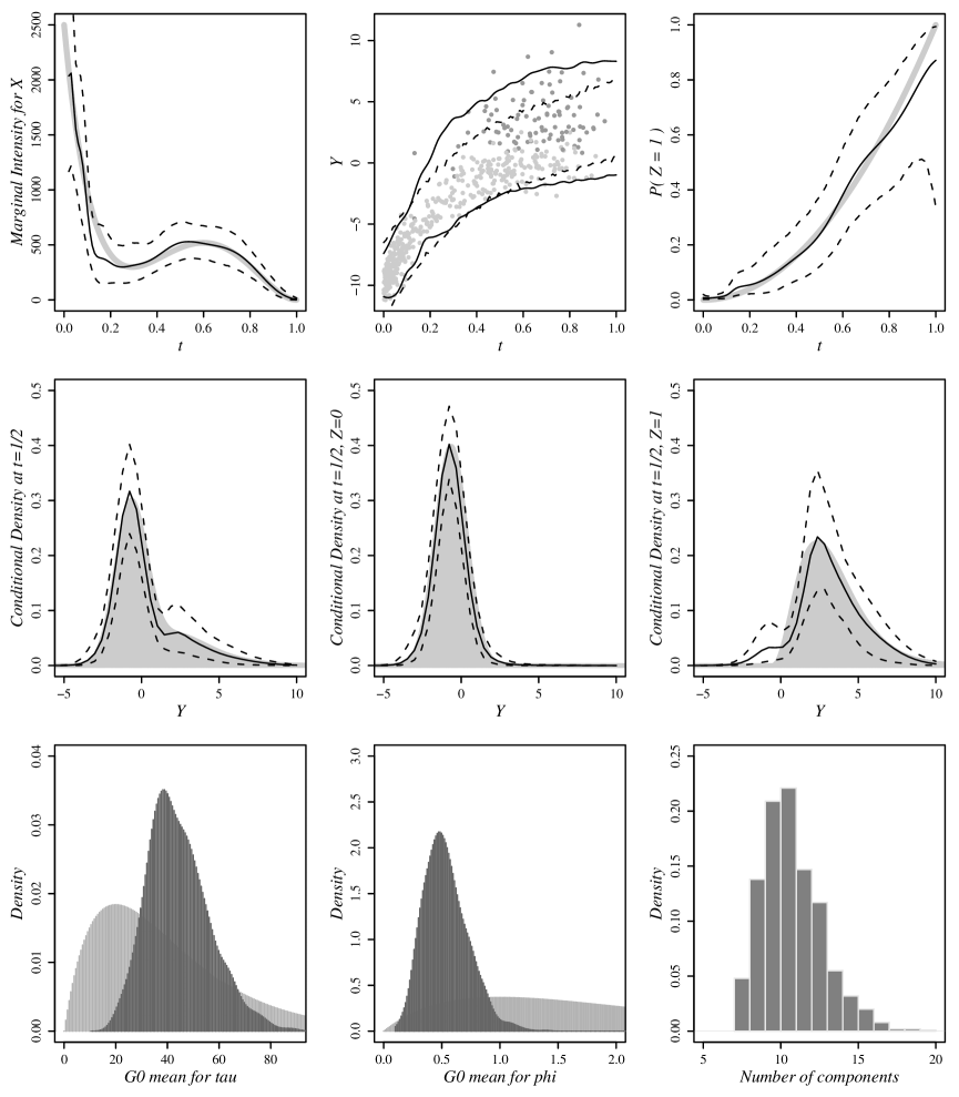
Figure 1: Simulation study results. On top, from left to right, we have posterior mean and 90% interval for the marginal intensity $\lambda(t;G)$ (with the true intensity denoted by the grey line), the data (dark grey for $z=1$), and posterior 90% predictive intervals based on both $h(y\mid t;G)$ (solid lines) and GP regression (dotted lines), and posterior mean and 90% intervals for $\mathrm{Pr}(z=1\mid t;G)$ (with the true function denoted by the grey line). The middle row has mean and 90% intervals for conditional densities for $y$ at $t=1/2$, marginalized over $z$ (left panel) and conditional on $z$ (middle and right panels), with true densities plotted in grey. Lastly, the bottom row shows posterior samples for $\beta_{\tau}$ and $\beta_{\phi}$ (dark grey, with priors in the background) and for the number of latent mixture components.

Results are shown in Figure 1. In the top row, we see that our methods are able to capture the marginal point intensity and general conditional behavior for $y$ and $z$; note that the uncertainty bounds are based on a full assessment of posterior uncertainty that is made possible through use of the truncated $G_{L}$ approximations to random mixing measure $G$ (as developed in Section 4.2). We also fit a Gaussian process (GP) regression model to the $(t,y)$ data pairs (using the tgp package for R under default parametrization) and, in contrast to our approach based on draws from $h(y\mid t;G_{L})$ as in (18), the top middle panel shows the GP model’s global variance as unable to adapt to a wider skewed error distribution for larger $t$ values.

The middle row of Figure 1 illustrates behavior for a slice of the conditional mark density for $y$, at $t=1/2$, both marginally and given $z=0$ or $1$. The marginal (left-most) plot shows that our model is able to reproduce the skewed response distribution, while the other two plots capture conditional response behavior given each value for $z$. As one would expect, posterior uncertainty around the conditional mark density estimates is highest at the transition from normal to gamma errors. Finally, posterior inference for model characteristics is illustrated in the bottom row of Figure 1. Peaked posteriors for $\beta_{\tau}$ and $\beta_{\phi}$ show that it is possible to learn about hyperparameters of the DP base distribution for both $t$ and $y$ kernel parameters, despite the flexibility of a DP mixture. Moreover, based on the posterior distribution for $m$, we note that the near to 500 observations have been shrunk to (on average) 12 distinct mixture components.

fnum@subsection5.2 Temporal Poisson process with count marks

Our second example involves a standard data set from the literature, the “coal-mining disasters” data (e.g., , Andrews and Herzberg1985, p. 53-56). The point pattern is defined by the times (in days) of 191 explosions of fire-damp or coal-dust in mines leading to accidents, involving 10 or more men killed, over a total time period of 40,550 days, from 15 March 1851 to 22 March 1962. The data marks $y$ are the number of deaths associated with each accident.

This example will compare two different mixture models for marginal location intensity: a “direct” model with beta-Poisson kernels, and a “transformed” model with data mapped to $\mathds{R}^{2}$ and fit via multivariate normal kernels. The first scheme models data directly on its original scale, but requires Metropolis-Hastings augmented MCMC for the beta kernel parameters, and dependence between $t$ and $y$ is induced only through $G$. The second model affords the convenience of the collapsed Gibbs sampler and correlated kernels, but on a transformed scale.

Following our general modeling approach, both models use the reference prior for $\Lambda_{\mathcal{R}}$ and assume NHPP density form $f(t,y;G)=$ $\int\mathrm{k}(t,y;\theta)dG(\theta)$ with $G\sim\mathrm{DP}(\alpha,G_{0})$ and $\pi(\alpha)=\mathrm{ga}(2,1)$. The distinction between the two models is thus limited to choice of kernel and base distribution. For the direct model,

$$\mathrm{k}(t,y;\mu,\tau,\phi) = b(t;\mu,\tau)\mathrm{Po}_{\geq 10}(y;\phi),$$ (20)

$$g_{0}(\mu,\tau,\phi) = \mathds{1}_{\mu\in(0,1)}\mathrm{ga}(\tau^{-1};2,\beta_{\tau})\mathrm{ga}(\phi;1,1/60),$$

where $\mathrm{Po}_{\geq 10}(y;\phi)$ is a Poisson density truncated at $y=10$, and with $\pi(\beta_{\tau})=\mathrm{ga}(1,1/63)$. This leads to prior expectations $\mathds{E}[\phi]=60$ and $\mathds{E}[\tau]=$ $\mathds{E}[\beta_{\tau}]=63$ for mean location kernel precision $(1+\tau)/(\mu(1-\mu))$ $\approx$ $4(1+63)$, which translates to a standard deviation of $1/16$. For the transformed model, we take $\tilde{y}=$ $y-9.5$ and

$$\mathrm{k}(t,y;\boldsymbol{\mu},\boldsymbol{\Sigma}) = \frac{\mathrm{N}\left([\mathrm{logit}(t),\log(\tilde{y})]^{\prime};\boldsymbol{\mu},\boldsymbol{\Sigma}\right)}{\tilde{y}t(1-t)}$$ (21)

$$g_{0}(\boldsymbol{\mu},\boldsymbol{\Sigma}) = \mathrm{N}(\boldsymbol{\mu};(0,2.5)^{\prime},10\boldsymbol{\Sigma})W(\boldsymbol{\Sigma}^{-1};3,\boldsymbol{\Omega}),$$

with $\pi(\boldsymbol{\Omega})=$ $\mathrm{W}(3,\mathrm{diag}[10,20])$ for $\mathds{E}(\Sigma)=$ $2/3\mathds{E}(\Omega)=\mathrm{diag}[1/5,1/10]$ ($\mathrm{logit}(t)$ and $\log(\tilde{y})$ range in (-5,5) and (-1,6), respectively). Both models were found to be robust to changes in this parametrization (e.g., $\mathds{E}[\phi]\in[10,100]$ and diagonal elements of $\mathds{E}[\Sigma]$ in $[0.1,1]$).

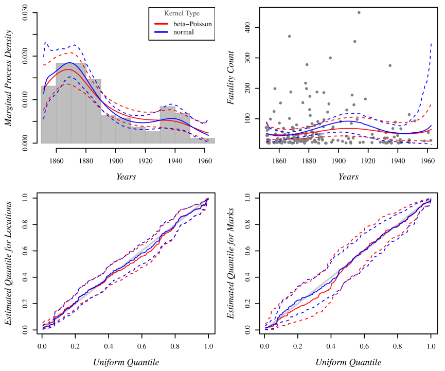
Figure 2: Coal-mining disasters. Mean and 90% intervals for (clockwise from top-left): marginal density $f(t;G_{L})$ (with data histogram); conditional expected count $\mathds{E}(y\mid t;G_{L})$ (data counts in grey); and posterior Q-Q plots for $\mathrm{Pr}(y<y_{i}\mid t_{i};G_{L})$ and $\Lambda(t_{i};G_{L})$, respectively.

Results under both models are shown in Figure 2. In the top left panel, we see that marginal process density estimates derived from each model are generally similar, with the normal model perhaps more sensitive to data peaks and troughs. There is no noticeable edge effect for either model. The Q-Q plot in the bottom left panel shows roughly similar fit with the normal model performing slightly better. The top and bottom right panels report inference for the count mark conditional mean and distribution Q-Q plot. For the beta-Poisson model, posterior realizations for $\mathds{E}(y\mid t;G_{L})$ are obtained using (19). The conditional mean calculation for the normal model must account for the correlated kernels (and the transformation to $\tilde{y}$), such that $\mathds{E}(y\mid t;G_{L})$ is 92 + (q_0∑_l=1^L p_l N(t; μ_lt, σ^2_lt) E[y ∣t;ϑ_l] + ∑_j=1^mq_jN(t; μ^⋆_jt, σ^⋆2_jt) E[y ∣t;θ^⋆_j])/f(t;G_L) where $\mathds{E}[y\mid t,\theta]=$ $\exp\left[\mu_{y}+\rho\sigma_{t}^{-2}(t-\mu_{t})+0.5(\sigma^{2}_{y}-\rho^{2}\sigma_{t}^{-2})\right]$ with $\boldsymbol{\mu}=$ $(\mu_{t},\mu_{y})$ and $\boldsymbol{\Sigma}$ partitioned into variances $(\sigma^{2}_{t},\sigma^{2}_{y})$ and correlation $\rho$. Similarly, uniform quantiles for the conditional mark distribution under the beta-Poisson model are available as weighted sums of Poisson distribution functions, while the normal model calculation for $\mathrm{Pr}(y<y_{i}\mid t_{i};G_{L})$ is as above for $\mathds{E}(y\mid t;G_{L})$, but with $\mathds{E}[y\mid t,\theta]$ replaced by $\mathrm{Pr}(y<y_{i}\mid t_{i};\theta)=$ $\Phi\left(\left[\tilde{y}_{i}-\mu_{y}+\rho\sigma_{t}^{-2}(t_{i}-\mu_{t})\right](\sigma^{2}_{y}-\rho^{2}\sigma_{t}^{-2})^{-1/2}\right)$. The estimated conditional mean functions are qualitatively different, with the poisson model missing the peak at WW1. Indeed, the corresponding QQ plot shows that the normal model provides a better fit to this data; we hypothesize that this is due to the equality of mean and variance assumed in Poisson kernels, and may be fixed by using instead, say, truncated negative binomials.

fnum@subsection5.3 Spatial Poisson process with continuous marks

Our final example considers the locations and diameters of 584 Longleaf pine trees in a $200\times 200$ meter patch of forest in Thomas County, GA. The trees were surveyed in 1979 and the measured mark is diameter at breast height (1.5 $m$), or $dbh$, recorded only for trees with greater than 2 cm dbh. The data, available as part of the spatstat package for R, were analyzed by Rathburn and Cressie (1994) as part of a space-time survival point process. Poisson processes are generally viewed as an inadequate model for forest patterns, due to the dependent birth process by which trees occur. However, the NHPP should be flexible enough to account for variability in tree counts at a single time point and, in this example, we will concentrate primarily on inference for the conditional $dbh$ mark distribution.

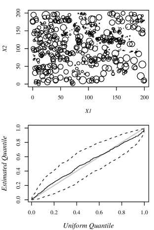
Figure 3: Longleaf pines. The left panel has data (point size proportional to tree diameter) and a Q-Q plot (mean and 90% interval) for $\int^{y}h(s\mid\mathbf{x};G_{L})ds$ evaluated at data. The right panel plots posterior mean and 90% intervals for $h(y\mid\mathbf{x};G_{L})$ at four specific $\mathbf{x}$ values.

To analyse this data set, we employ a spatial version of the model in (13), with tree marks log-transformed to lie on the real line. Thus, our three-dimensional normal kernel model is

$$\phi(\mathbf{x},y;G)=\Lambda_{\mathcal{R}}\int\frac{\mathrm{N}\left([\mathrm{logit}(\mathbf{x}),\log(y-2)]^{\prime};\boldsymbol{\mu},\boldsymbol{\Sigma}\right)}{(y-2)\prod_{i=1}^{2}x_{i}(1-x_{i})}dG(\boldsymbol{\mu},\boldsymbol{\Sigma}),\hskip 14.22636ptG\sim\mathrm{DP}(\alpha,G_{0}).$$

The base distribution is taken to be $g_{0}(\boldsymbol{\mu},\boldsymbol{\Sigma})=$ $\mathrm{N}(\boldsymbol{\mu};(0,0,1)^{\prime},100\boldsymbol{\Sigma})\mathrm{W}(\boldsymbol{\Sigma}^{-1};4,\boldsymbol{\Omega})$, with $\pi(\boldsymbol{\Omega})=$ $\mathrm{W}(4,\mathrm{diag}[0.1,0.1,0.1,0.1])$. A $\mathrm{ga}(2,1)$ prior is placed on $\alpha$. Posterior sampling follows the fully collapsed Gibbs algorithm of Appendix A.2.

In this data set, high density clusters of juveniles trees (dbh $<5$cm) combine with the more even dispersal of larger trees to form conditional mark densities with non-standard shapes and non-homogeneous variability. This behavior is clearly exhibited in the posterior estimates of the conditional density for $dbh$, shown on the right side of Figure 3, at four different locations in the observations window. Although conditional densities vary in shape over the different locations, each appears to show the mixture of a diffuse component for mature trees combined with a sharp increase in density at low $dbh$ values, corresponding to collections of juvenile trees (only some of whom make it to maturity). It is notable that we are able to infer this structure nonparametrically, in contrast to existing approaches where the effect of a tree-age threshold is assumed a priori (as in Rathburn and Cressie, 1994). Finally, the conditional mark distribution Q-Q plot on the bottom right panel of Figure 3 (based on calculations similar to those in Section 5.2) shows a generally decent mean-fit with wide uncertainty bands corresponding to the 95% and 5% density percentile Q-Q plots.

6 Discussion

We have presented a nonparametric Bayesian modeling framework for marked non-homogeneous Poisson processes. The key feature of the approach is that it develops the modeling from the Poisson process density. We have considered various forms of Dirichlet process mixture models for this density which, when extended to the joint mark-location process, result in highly flexible nonparametric inference for the location intensity as well as for the conditional mark distribution. The approach enables modeling and inference for multivariate mark distributions comprising both categorical and continuous marks, and is especially appealing with regard to the relative simplicity with which it can accommodate spatially correlated marks. We have discussed methods for prior specification, posterior simulation and inference, and model checking. Finally, three data examples were used to illustrate the proposed methodology.

The Poisson assumption for marked point processes is what enables us to separate modeling for the process density from the integrated intensity. This simplification is particularly useful for applications involving several related intensity functions and mark distributions, and is less restrictive than it may at first appear. For instance, Taddy (2010) presents an estimation of weekly violent crime intensity surfaces, using autoregressive modeling for marked spatial NHPPs, and (Kottas et al.2011) compares neuronal firing intensities recorded under multiple experimental conditions, using hierarchically dependent modeling for temporal NHPPs.

Among the possible ways to relax the restrictions of the Poisson assumption, while retaining the appealing structure of the NHPP likelihood, we note the class of multiplicative intensity models studied, for instance, in Ishwaran and James (2004). These models for marked point processes are under the NHPP setting and, indeed, follow the simpler strategy of separate modeling for the process intensity and mark density as in the semiparametric framework of Section 3.1. More generally, one could envision relaxing the Poisson assumption for the number of marks through a joint intensity function such that the location intensity is not the marginal of the joint intensity over marks. Such extensions would however sacrifice the main feature of our proposed framework – flexible modeling for multivariate mark distributions under a practical posterior simulation inference scheme. As a more basic extension, our factorization in (1) could be combined with alternative specifications for integrated intensity; for example, hierarchical models may be useful to connect intensity across observation windows.

Appendix: Implementation Details for Dirichlet Process Mixture Models

A.1   Prior Specification

Prior specification for the DP precision parameter is facilitated by the role of $\alpha$ in controlling the number, $m\leq N$, of distinct mixture components. For instance, for moderately large $N$, $\mathds{E}[m\mid\alpha]\approx$ $\alpha\log\left((\alpha+N)/\alpha\right)$. Furthermore, it is common to assume a gamma prior for $\alpha$, such that $\pi(\alpha)=$ $\mathrm{ga}(\alpha;a_{\alpha},b_{\alpha})$, and use prior intuition about $m$ combined with $\mathds{E}[m\mid\alpha]$ to guide the choice of $a_{\alpha}$ and $b_{\alpha}$.

Specification of the base distribution parameters will clearly depend on kernel choice and application details, and DP mixture models are typically robust to reasonable changes in this specification. First, the base distribution for kernel location (usually the mean, but possibly median) can be specified through a prior guess for the data center; for example, this value can be used to fix the mean parameter $\boldsymbol{\delta}$ in (6) or the mean of a normal hyperprior for $\boldsymbol{\delta}$. In choosing dispersion parameters, note that the DP prior will place most mass on a small number of mixture components, with the remaining components assigned very little weight and, hence, very few observations. At the same time, this behavior can be overcome in the posterior and it is important to not restrict the mixture to overly-dispersed kernels. Thus, the expectation of the kernel variance (or scale, or shape) parameters should be specified with a small number of mixture components in mind, but with low precision. For example, again in the context of (6), the square-root of the hyperprior expectation for diagonal elements of $\boldsymbol{\Omega}$ can be set at $1/8$ to $1/16$ of a prior guess at data range, and the precision $\nu$ will be as small as is practical (usually the dimension of the kernel plus 2). The factor $\kappa$ is then chosen to scale the mixture to expected dispersion in $\boldsymbol{\mu}$.

Moreover, except when specific prior information about co-dependence is available, it is best to center $G_{0}$ on kernel parametrization that implies independence between variables, such that the mixture is centered on a model with dependence induced nonparametrically by $G$. For example, in the model of (6), we assume zeros in the off-diagonal elements for the prior expectation of $\boldsymbol{\Omega}$, and this is combined with a small $\nu$ to allow for within-kernel dependence where appropriate. A prior expectation of independence also fits with our general approach of building kernels for mixed-type data as the product of multiple independent densities.

Note that we have chosen to introduce prior information into the base measure based on the intuition arising from a small number of large mixture components and $\alpha$ near zero. Recent work in Bush, Lee, and MacEachern (2010) provides a rigorous treatment of non-informative prior specification, and they advocate a hierarchical scheme for $\alpha|G_{0}$ that maintains desirable properties at all scales of precision. As the main work here – use of mixtures for modeling joint location-mark Poisson process densities – is independent of prior and base measure choice, these innovations, as well as application-specific prior schemes, could potentially be integrated into our framework.

A.2   Posterior Simulation

Using results from Antoniak (1974), the posterior distribution for the DP mixture model is partitioned as $\mathrm{p}(G,\boldsymbol{\theta}^{\star},\mathbf{s},\alpha,\psi\mid\text{data})=$ $\mathrm{p}(G\mid\boldsymbol{\theta}^{\star},\mathbf{s},\alpha,\psi)\mathrm{p}(\boldsymbol{\theta}^{\star},\mathbf{s},\alpha,\psi\mid\text{data})$, where $G$, given $\boldsymbol{\theta}^{\star},\mathbf{s},\alpha,\psi$, is distributed as a DP with precision parameter $\alpha+N$ and base distribution given by (15). Hence, full posterior inference involves sampling for the finite dimensional portion of the parameter vector, which is next supplemented with draws from the conditional posterior distribution for $G$ (obtained as discussed in Section 4.2). A generic Gibbs sampler for posterior simulation from $\mathrm{p}(\boldsymbol{\theta}^{\star},\mathbf{s},\alpha,\psi\mid\text{data})$, derived by combining MCMC methods from MacEachern (1994) and Escobar and West (1995), proceeds iteratively as follows:

• For $i=1,\ldots,N$, denote by $\mathbf{s}^{(-i)}$ the allocation vector with component $s_{i}$ removed, and by $N_{s}^{(-i)}$ the number of elements of $\mathbf{s}^{(-i)}$ that are equal to $s$. Then, if $s=s_{r}$ for some $r\neq i$, the $i$-th allocation variable is updated according to Pr(s_i = s ∣s^(-i),α,ψ,data) ∝Ns(-i)N - 1 + α ∫k(z_i;θ^⋆) p(θ^⋆ ∣s^(-i),ψ,data) dθ^⋆, where $p(\theta^{\star}\mid\mathbf{s}^{(-i)},\psi,\text{data})$ is the density proportional to $g_{0}(\theta^{\star};\psi)\prod\nolimits_{\{r\neq i:s_{r}=s\}}\mathrm{k}(\mathbf{z}_{r};\theta^{\star})$. Moreover, the probability of generating a new component, that is, $\text{Pr}(s_{i}\neq s_{r}\,\text{for all}\,r\neq i\mid\mathbf{s}^{(-i)},\alpha,\psi,\text{data})$, is proportional to $\alpha(N-1+\alpha)^{-1}\int\mathrm{k}(\mathbf{z}_{i};\theta^{\star})g_{0}(\theta^{\star};\psi)d\theta^{\star}$.

• For $j=1,...,m$, draw $\theta^{\star}_{j}$ from $p(\theta^{\star}_{j}\mid\mathbf{s},\psi,\text{data})\propto$ $g_{0}(\theta^{\star}_{j};\psi)\prod\nolimits_{\{i:s_{i}=j\}}\mathrm{k}(\mathbf{z}_{i};\theta^{\star}_{j})$.

• Draw the base distribution hyperparameters from $\pi(\psi)\prod_{j=1}^{m}g_{0}(\theta^{\star}_{j};\psi)$, where $\pi(\psi)$ is the prior for $\psi$. Finally, if $\alpha$ is assigned a gamma hyperprior, it can be updated conditional on only $m$ and $N$ using the auxiliary variable method from Escobar and West (1995).

The integrals that are needed to update the components of $\mathbf{s}$ can be evaluated analytically for models where $G_{0}$ is conjugate for $\mathrm{k}(\cdot;\theta)$. It is for this reason that conditionally conjugate mixture models can lead to substantially more efficient posterior sampling, especially when $\theta$ is high-dimensional. When this is not true (as for, e.g., beta kernel models or the truncated Poisson of Equation 20), the draw for $\mathbf{s}$ requires use of the auxiliary parameters, $\boldsymbol{\theta}^{\star}$, sampled as in the second step of our algorithm, in conjunction with a joint Metropolis-Hastings draw for each $\theta_{i}$ and $s_{i}$ given $\boldsymbol{\theta}^{(-i)}$ and $\mathbf{s}^{(-i)}$. In particular, we can make use of algorithms from Neal (2000) for non-conjugate models.

References

- (1) Andrews, D. F. and Herzberg, A. M. (1985). Data, A Collection of Problems from Many Fields for the Student and Research Worker. Springer-Verlag.
- Antoniak (1974) Antoniak, C. (1974). Mixtures of Dirichlet processes with applications to Bayesian nonparametric problems. Annals of Statistics 2, 1152 – 1174.
- Baddeley et al. (2005) Baddeley, A., R. Turner, J. Møller, and M. Hazelton (2005). Residual analysis for spatial point processes (with discussion). Journal of the Royal Statistical Society, Series B 67, 617–666.
- Best et al. (2000) Best, N. G., K. Ickstadt, and R. L. Wolpert (2000). Spatial Poisson regression for health and exposure data measured at disparate resolutions. Journal of the American Statistical Association 95, 1076–1088.
- Brix and Diggle (2001) Brix, A. and P. J. Diggle (2001). Spatiotemporal prediction for log-Gaussian Cox processes. Journal of the Royal Statistical Society, Series B 63, 823–841.
- Brix and Møller (2001) Brix, A. and J. Møller (2001). Space-time multi type log Gaussian Cox processes with a view to modeling weeds. Scandinavian Journal of Statistics 28, 471–488.
- Brown et al. (2001) Brown, E. M., R. Barbieri, V. Ventura, R. E. Kass, and L. M. Frank (2001). The time-rescaling theorem and its application to neural spike train data analysis. Neural Computation 14, 325–346.
- Brunner and Lo (1989) Brunner, L. J. and A. Y. Lo (1989). Bayes methods for a symmetric uni-modal density and its mode. Annals of Statistics 17, 1550–1566.
- Bush, Lee, and MacEachern (2010) Bush, C., J. Lee, and S. N. MacEachern (2010). Minimally informative prior distributions for nonparametric Bayesian analysis. Journal of the Royal Statistical Society: Series B 72, 253–268.
- Cressie (1993) Cressie, N. A. C. (1993). Statistics for Spatial Data (Revised edition). Wiley.
- Daley and Vere-Jones (2003) Daley, D. J. and D. Vere-Jones (2003). An Introduction to the Theory of Point Processes (2nd ed.). Springer.
- Diaconis and Ylvisaker (1985) Diaconis, P. and D. Ylvisaker (1985). Quantifying prior opinion. In J. M. Bernardo, M. H. DeGroot, D. V. Lindley, and A. F. M. Smith (Eds.), Bayesian Statistics, Volume 2. North-Holland.
- Diggle (1990) Diggle, P. J. (1990). A point process modelling approach to raised incidence of a rare phenomenon in the vicinity of a prespecified point. Journal of the Royal Statistical Society, Series A 153, 349–362.
- Diggle (2003) Diggle, P. J. (2003). Statistical Analysis of Spatial Point Patterns (Second Edition). London, Arnold.
- Escobar and West (1995) Escobar, M. and M. West (1995). Bayesian density estimation and inference using mixtures. Journal of the American Statistical Association 90, 577–588.
- Ferguson (1973) Ferguson, T. (1973). A Bayesian analysis of some nonparametric problems. Annals of Statistics 1, 209–230.
- Grunwald et al. (1993) Grunwald, G. K., A. E. Raftery, and P. Guttorp (1993). Time series of continuous proportions. Journal of the Royal Statistical Society, Series B 55, 103–116.
- Gutiérrez-Peña and Nieto-Barajas (2003) Gutiérrez-Peña, E. and L. E. Nieto-Barajas (2003). Bayesian nonparametric inference for mixed Poisson processes. In J. Bernardo, M. Bayarri, J. Berger, A. Dawid, D. Heckerman, A. Smith, and M. West (Eds.), Bayesian Statistics 7, pp. 163–179. Oxford Univeresity Press.
- Guttorp (1995) Guttorp, P. (1995). Stochastic Modelling of Scientific Data. Chapman & Hall.
- Heikkinen and Arjas (1998) Heikkinen, J. and E. Arjas (1998). Non-parametric Bayesian estimation of a spatial Poisson intensity. Scandinavian Journal of Statistics 25, 435–450.
- Heikkinen and Arjas (1999) Heikkinen, J. and E. Arjas (1999). Modeling a Poisson forest in variable elevations: a nonparametric Bayesian approach. Biometrics 55, 738–745.
- Hjort (1990) Hjort, N. L. (1990). Nonparametric Bayes Estimators based on beta processes in models for life history data. Annals of Statistics 18, 1259–1294.
- Ickstadt and Wolpert (1999) Ickstadt, K. and R. L. Wolpert (1999). Spatial regression for marked point processes. In J. M. Bernardo, J. O. Berger, P. Dawid, and A. F. M. Smith (Eds.), Bayesian Statistics 6, pp. 323–341. Oxford University Press.
- Ishwaran and James (2004) Ishwaran, H. and L. F. James (2004). Computational methods for multiplicative intensity models using weighted gamma processes: Proportional hazards, marked point processes, and panel count data. Journal of the American Statistical Association 99, 175–190.
- Ishwaran and Zarepour (2002) Ishwaran, H. and M. Zarepour (2002). Exact and approximate sum representations for the Dirichlet process. The Canadian Journal of Statistics 30, 269–283.
- Ji et al. (2009) Ji, C., D. Merl, T. B. Kepler, and M. West (2009). Spatial mixture modelling for unobserved point processes: Examples in immunofluorescence histology. Bayesian Analysis 4, 297 – 316.
- Kingman (1993) Kingman, J. F. C. (1993). Poisson Processes. Clarendon Press.
- Kottas and Gelfand (2001) Kottas, A. and A. E. Gelfand (2001). Bayesian semiparametric median regression modeling. Journal of the American Statistical Association 96, 1458–1468.
- Kottas and Sansó (2007) Kottas, A. and B. Sansó (2007). Bayesian mixture modeling for spatial Poisson process intensities, with applications to extreme value analysis. Journal of Statistical Planning and Inference 137, 3151–3163.
- Kottas and Behseta (2010) Kottas, A. and S. Behseta (2010). Bayesian nonparametric modeling for comparison of single-neuron firing intensities. Biometrics 66, 277–286.
- (31) Kottas, A., S. Behseta, D. E. Moorman, V. Poynor, and C. R. Olson (2011). Bayesian nonparametric analysis of neuronal intensity rates. Journal of Neuroscience Methods, in press; doi:10.1016/j.jneumeth.2011.09.017
- Kuo and Ghosh (1997) Kuo, L. and S. K. Ghosh (1997). Bayesian nonparametric inference for nonhomogeneous Poisson processes. Technical report, Department of Statistics, University of Connecticut.
- Kuo and Yang (1996) Kuo, L. and T. Y. Yang (1996). Bayesian computation for nonhomogeneous Poisson processes in software reliability. Journal of the American Statistical Association 91, 763–773.
- Liang et al. (2009) Liang, S., B. P. Carlin, and A. E. Gelfand (2009). Analysis of Minnesota colon and rectum cancer point patterns with spatial and nonspatial covariate information. The Annals of Applied Statistics 3, 943–962.
- Lo (1992) Lo, A. Y. (1992). Bayesian inference for Poisson process models with censored data. Journal of Nonparametric Statistics 2, 71–80.
- Lo and Weng (1989) Lo, A. Y. and C.-S. Weng (1989). On a class of Bayesian nonparametric estimates: II. Hazard rate estimates. Annals of the Institute for Statistical Mathematics 41, 227–245.
- MacEachern (1994) MacEachern, S. N. (1994). Estimating normal means with a conjugate style Dirichlet process prior. Communications in Statistics: Simulation and Computation 23, 727–741.
- MacEachern et al. (1999) MacEachern, S. N., M. Clyde, and J. S. Liu (1999). Sequential importance sampling for nonparametric Bayes models: The next generation. The Canadian Journal of Statistics 27, 251–267.
- Møller et al. (1998) Møller, J., A. R. Syversveen, and R. P. Waagepetersen (1998). Log Gaussian Cox processes. Scandinavian Journal of Statistics 25, 451–452.
- Møller and Waagepetersen (2004) Møller, J. and R. P. Waagepetersen (2004). Statistical Inference and Simulation for Spatial Point Processes. Chapman & Hall/CRC.
- Müller et al. (1996) Müller, P., A. Erkanli, and M. West (1996). Bayesian curve fitting using multivariate normal mixtures. Biometrika 83, 67–79.
- Neal (2000) Neal, R. (2000). Markov chain sampling methods for Dirichlet process mixture models. Journal of Computational and Graphical Statistics 9, 249–265.
- Pitman (1996) Pitman, J. (1996). Some developments of the Blackwell-MacQueen urn scheme. In T. S. Ferguson, L. S. Shapley, and J. B. MacQueen (Eds.), Statistics, Probability and Game Theory, IMS Lecture Notes – Monograph Series, 30, pp. 245–267.
- Rathburn and Cressie (1994) Rathburn, S. L. and N. Cressie (1994). A space-time survival point process for a longleaf pine forest in southern Georgia. Journal of the American Statistical Association 89, 1164–1174.
- Rodriguez et al. (2009) Rodriguez, A., D. B. Dunson, and A. E. Gelfand (2009). Nonparametric functional data analysis through Bayesian density estimation. Biometrika 96, 149–162.
- Sethuraman (1994) Sethuraman, J. (1994). A constructive definition of the Dirichlet prior. Statistica Sinica 4, 639–650.
- Taddy (2010) Taddy, M. (2010). Autoregressive mixture models for dynamic spatial Poisson processes: Application to tracking intensity of violent crime Journal of the American Statistical Association 105, 1403–1417.
- Taddy and Kottas (2010) Taddy, M. and A. Kottas (2010). A Bayesian nonparametric approach to inference for quantile regression. Journal of Business and Economic Statistics 28, 357–369.
- Wolpert and Ickstadt (1998) Wolpert, R. L. and K. Ickstadt (1998). Poisson/gamma random field models for spatial statistics. Biometrika 85, 251–267.