The Exact String Matching Problem:
a Comprehensive Experimental Evaluation

Abstract

This paper addresses the online exact string matching problem which consists in finding all occurrences of a given pattern $p$ in a text $t$. It is an extensively studied problem in computer science, mainly due to its direct applications to such diverse areas as text, image and signal processing, speech analysis and recognition, data compression, information retrieval, computational biology and chemistry. Since 1970 more than 80 string matching algorithms have been proposed, and more than 50% of them in the last ten years. In this note we present a comprehensive list of all string matching algorithms and present experimental results in order to compare them from a practical point of view. ¿From our experimental evaluation it turns out that the performance of the algorithms are quite different for different alphabet sizes and pattern length.

1 Introduction

Given a text $t$ of length $n$ and a pattern $p$ of length $m$ over some alphabet $\Sigma$ of size $\sigma$, the string matching problem consists in finding all occurrences of the pattern $p$ in the text $t$. It is an extensively studied problem in computer science, mainly due to its direct applications to such diverse areas as text, image and signal processing, speech analysis and recognition, data compression, information retrieval, computational biology and chemistry.

String matching algorithms are also basic components used in implementations of practical softwares existing under most operating systems. Moreover, they emphasize programming methods that serve as paradigms in other fields of computer science. Finally they also play an important role in theoretical computer science by providing challenging problems.

Applications require two kinds of solutions depending on which string, the pattern or the text, is given first. Algorithms based on the use of automata or combinatorial properties of strings are commonly implemented to preprocess the pattern and solve the first kind of problem. This kind of problem is generally referred as online string matching. The notion of indexes realized by trees or automata is used instead in the second kind of problem, generally referred as offline string matching. In this paper we are only interested in algorithms of the first kind.

The worst case lower bound of the online string matching problem is $\mathcal{O}(n)$ and has been firstly reached by the well known Morris-Pratt algorithm [MP70]. An average lower bound in $\mathcal{O}(n\log m/m)$ (with equiprobability and independence of letters) has been proved by Yao in [Yao79].

Algorithms based on characters comparison
BF	Brute-Force	[CLRS01]
MP	Morris-Pratt	[MP70]	1970
KMP	Knuth-Morris-Pratt	[KMP77]	1977
BM	Boyer-Moore	[BM77]	1977
HOR	Horspool	[Hor80]	1980
GS	Galil-Seiferas	[GS83]	1983
AG	Apostolico-Giancarlo	[AG86]	1986
KR	Karp-Rabin	[KR87]	1987
ZT	Zhu-Takaoka	[ZT87]	1987
OM	Optimal-Mismatch	[Sun90]	1990
MS	Maximal-Shift	[Sun90]	1990
QS	Quick-Search	[Sun90]	1990
AC	Apostolico-Crochemore	[AC91]	1991
TW	Two-Way	[CP91]	1991
TunBM	Tuned-Boyer-Moore	[HS91]	1991
COL	Colussi	[Col91]	1991
SMITH	Smith	[Smi91]	1991
GG	Galil-Giancarlo	[GG92]	1992
RAITA	Raita	[Rai92]	1992
SMOA	String-Matching on Ordered ALphabet	[Cro92]	1992
NSN	Not-So-Naive	[Han93]	1993
TBM	Turbo-Boyer-Moore	[CCG+94]	1994
RCOL	Reverse-Colussi	[Col94]	1994
SKIP	Skip-Search	[CLP98]	1998
ASKIP	Alpha-Skip-Search	[CLP98]	1998
KMPS	KMP-Skip-Search	[CLP98]	1998
BR	Berry-Ravindran	[BR99]	1999
AKC	Ahmed-Kaykobad-Chowdhury	[AKC03]	2003
FS	Fast-Search	[CF03]	2003
FFS	Forward-Fast-Search	[CF05]	2004
BFS	Backward-Fast-Search, Fast-Boyer-Moore	[CF05, CL08]	2004
TS	Tailed-Substring	[CF04]	2004
SSABS	Sheik-Sumit-Anindya-Balakrishnan-Sekar	[SAP+04]	2004
TVSBS	Thathoo-Virmani-Sai-Balakrishnan-Sekar	[TVL+06]	2006
PBMH	Boyer-Moore-Horspool using Probabilities	[Neb06]	2006
FJS	Franek-Jennings-Smyth	[FJS07]	2007
2BLOCK	2-Block Boyer-Moore	[SM07]	2007
HASH$q$	Wu-Manber for Single Pattern Matching	[Lec07]	2007
TSW	Two-Sliding-Window	[HAKS+08]	2008
BMH$q$	Boyer-Moore-Horspool with $q$-grams	[KPT08]	2008
GRASPm	Genomic Rapid Algo for String Pm	[DC09]	2009
SSEF	SSEF	[Kül09]	2009

Figure 1: The list of all comparison based string matching algorithms (1970-2010).

Algorithms based on automata
DFA	Deterministic-Finite-Automaton	[CLRS01]
RF	Reverse-Factor	[Lec92]	1992
SIM	Simon	[Sim93]	1993
TRF	Turbo-Reverse-Factor	[CCG+94]	1994
FDM	Forward-DAWG-Matching	[CR94]	1994
BDM	Backward-DAWG-Matching	[CR94]	1994
BOM	Backward-Oracle-Matching	[ACR99]	1999
DFDM	Double Forward DAWG Matching	[AR00]	2000
WW	Wide Window	[HFS05]	2005
LDM	Linear DAWG Matching	[HFS05]	2005
ILDM1	Improved Linear DAWG Matching	[LWLL06]	2006
ILDM2	Improved Linear DAWG Matching 2	[LWLL06]	2006
EBOM	Extended Backward Oracle Matching	[FL08]	2009
FBOM	Forward Backward Oracle Matching	[FL08]	2009
SEBOM	Simplified Extended Backward Oracle Matching	[FYM09]	2009
SFBOM	Simplified Forward Backward Oracle Matching	[FYM09]	2009
SBDM	Succint Backward DAWG Matching	[Fre09]	2009

Figure 2: The list of the automata based string matching algorithms (1992-2009).

Algorithms based on bit-parallelism
SO	Shift-Or	[BYR92]	1992
SA	Shift-And	[BYR92]	1992
BNDM	Backward-Nondeterministic-DAWG-Matching	[NR98a]	1998
BNDM-L	BNDM for Long patterns	[NR00]	2000
SBNDM	Simplified BNDM	[PT03, Nav01]	2003
TNDM	Two-Way Nondeterministic DAWG Matching	[PT03]	2003
LBNDM	Long patterns BNDM	[PT03]	2003
SVM	Shift Vector Matching	[PT03]	2003
BNDM2	BNDM with loop-unrolling	[HD05]	2005
SBNDM2	Simplified BNDM with loop-unrolling	[HD05]	2005
BNDM-BMH	BNDM with Horspool Shift	[HD05]	2005
BMH-BNDM	Horspool with BNDM test	[HD05]	2005
FNDM	Forward Nondeterministic DAWG Matching	[HD05]	2005
BWW	Bit parallel Wide Window	[HFS05]	2005
FAOSO	Fast Average Optimal Shift-Or	[FG05]	2005
AOSO	Average Optimal Shift-Or	[FG05]	2005
BLIM	Bit-Parallel Length Invariant Matcher	[Kül08]	2008
FSBNDM	Forward SBNDM	[FL08]	2009
BNDM$q$	BNDM with $q$-grams	[DHPT09]	2009
SBNDM$q$	Simplified BNDM with $q$-grams	[DHPT09]	2009
UFNDM$q$	Shift-Or with $q$-grams	[DHPT09]	2009
SABP	Small Alphabet Bit-Parallel	[ZZMY09]	2009
BP2WW	Bit-Parallel2 Wide-Window	[CFG10a]	2010
BPWW2	Bit-Parallel Wide-Window2	[CFG10a]	2010
KBNDM	Factorized BNDM	[CFG10b]	2010
KSA	Factorized Shift-And	[CFG10b]	2010

Figure 3: The list of all bit-parallel string matching algorithms (1992-2010).

More than 80 online string matching algorithms (hereafter simply string matching algorithms) have been proposed over the years. All solutions can be divided into two classes: algorithms which solve the problem by making use only of comparisons between characters, and algorithms which make use of automata in order to locate all occurrences of the searched string. The latter class can be further divided into two classes: algorithms which make use of deterministic automata and algorithms based on bit-parallelism which simulate the behavior of non-deterministic automata.

Fig. 1, Fig. 2 and Fig. 3 present the list of all string matching algorithms based on comparison of characters, deterministic automata and bit-parallelism, respectively.

The class of algorithms based on comparison of characters is the wider class and consists of almost 50 per cent of all solutions. Among the comparison based string matching algorithms the Boyer-Moore algorithm [BM77] deserves a special mention, since it has been particularly successful and has inspired much work.

Also automata play a very important role in the design of efficient string matching algorithms. The first linear algorithm based on deterministic automata is the Automaton Matcher [CLRS01].

Over the years automata based solutions have been also developed to design algorithms which have optimal sublinear performance on average. This is done by using factor automata [BBE⁺83, Cro85, BBE⁺85, ACR99], data structures which identify all factors of a word. Among the algorithms which make use of a factor automaton the BDM [CR94] and the Backward-Oracle-Matching algorithm [ACR99] are among the most efficient solutions, especially for long patterns.

In recent years, most of the work has been devoted to develop software techniques to simulate efficiently the parallel computation of non-deterministic finite automata related to the search pattern. Such simulations can be done efficiently using the bit-parallelism technique [BYG92], which consists in exploiting the intrinsic parallelism of the bit operations inside a computer word. In some cases, bit-parallelism allows to reduce the overall number of operations up to a factor equal to the number of bits in a computer word. Thus, although string matching algorithms based on bit-parallelism are usually simple and have very low memory requirements, they generally work well with patterns of moderate length only.

The bit-parallelism technique has been used to simulate efficiently the non-deterministic version of the Morris-Pratt automaton. The resulting algorithm, named Shift-Or [BYG92], runs in $\mathcal{O}(n\lceil m/w\rceil)$, where $w$ is the number of bits in a computer word. Later, a variant of the Shift-Or algorithm, called Shift-And, and a very fast BDM-like algorithm (BNDM), based on the bit-parallel simulation of the non-deterministic suffix automaton, were presented in [NR98b].

Bit-parallelism encoding requires one bit per pattern symbol, for a total of $\lceil m/w\rceil$ computer words. Thus, as long as a pattern fits in a computer word, bit-parallel algorithms are extremely fast, otherwise their performance degrades considerably as $\lceil m/w\rceil$ grows. Though there are a few techniques to maintain good performance in the case of long patterns, such limitation is intrinsic.

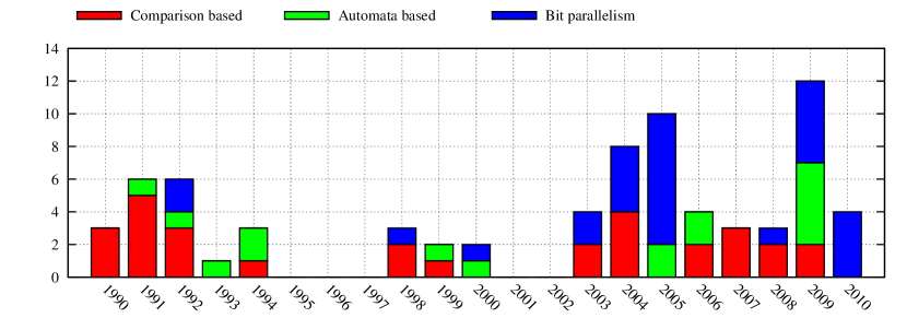
Figure 4: Number of algorithms proposed in the last 21 years (1990-2010)

Fig. 4 presents a plot of the number of algorithms (for each class) proposed in the last 21 years (1990-2010). Observe that the number of proposed solutions have doubled in the last ten years, demonstrating the increasing interest in this issue. It is interesting to observe also that almost 50 per cent of solutions in the last ten years are based on bit-parallelism. Moreover it seems that the number of bit-parallel solutions proposed in the years follows an increasing trend.

In the rest of the paper we present a comprehensive experimental evaluation of all string matching algorithms listed above in order to compare them from a practical point of view.

2 Experimental Results

We present next experimental data which allow to compare in terms of running time all the algorithms listed in Fig. 1, Fig. 2 and Fig. 3.

In particular we tested the Hash$q$ algorithm with $q$ equal to $3$, $5$ and $8$. The AOSO and BNDM$q$ algorithms have been tested with a value of $q$ equal to $2$, $4$ and $6$. Finally the SBNDM$q$ and UFNDM$q$ have been tested with $q$ equal to $2$, $4$, $6$ and $8$.

All algorithms have been implemented in the C programming language and were used to search for the same strings in large fixed text buffers on a PC with Intel Core2 processor of 1.66GHz and running times have been measured with a hardware cycle counter, available on modern CPUs. The codes have been compiled with the GNU C Compiler, using the optimization options -O2 -fno-guess-branch-probability.

In particular, the algorithms have been tested on the following 12 text buffers:

1. eight Rand$\sigma$ text buffers, for $\sigma=2,4,8,16,32,64,128$ and $256$, where each Rand$\sigma$ text buffer consists in a 5Mb random text over a common alphabet of size $\sigma$, with a uniform distribution of characters;

2. a genome sequence of $4,638,690$ base pairs of Escherichia coli (with $\sigma=4$);

3. a protein sequence (the hs file) from the Saccharomyces cerevisiae genome, of length $3,295,751$ byte (with $\sigma=20$);

4. the English King James version of the Bible composed of $4,047,392$ characters (with $\sigma=63$);

5. the file world192.txt (The CIA World Fact Book) composed of $2,473,400$ characters (with $\sigma=94$);

Files (ii), (iv) and (v) are from the Large Canterbury Corpus (http://www.data-compression.info/Corpora/CanterburyCorpus/), while file (iii) is from the Protein Corpus (http://data-compression.info/Corpora/ProteinCorpus/).

For each input file, we have generated sets of 400 patterns of fixed length $m$ randomly extracted from the text, for $m$ ranging over the values $2$, $4$, $8$, $16$, $32$, $64$, $128$, $256$, $512$ and $1024$. For each set of patterns we reported in a table the mean over the running times of the 400 runs. Running times are expressed in thousandths of seconds.

Moreover we color each running time value with different shades of blue-red. In particular better results are presented in tones verging to red while worse results are presented in tones verging to blue. In addition best results are highlighted with a light gray background.

Although we tested more than 85 different algorithms, for the sake of clearness we include in the following tables only the algorithms that obtain, for each text buffer and each pattern length, the 25 best results. We add a red marker to comparison based algorithms, while a green and a blue marker is added to automata and bit parallel algorithms, respectively.

Then, for each table, we briefly discuss the performance of the string matching algorithms by referring to the following four classes of patterns:

• very short patterns (pattern with $m\leq 4$);

• short patterns (pattern with $4<m\leq 32$);

• long patterns (pattern with $32<m\leq 256$);

• very long patterns (pattern with $m>256$);

Finally we discuss the overall performance of the tested algorithms by considering those algorithms which maintain good performance for all classes of patterns.

2.1 Experimental Results on Rand$2$ Problem

In this section we present experimental results on a random text buffer over a binary alphabet. Matching binary data is an interesting problem in computer science, since binary data are omnipresent in telecom and computer network applications. Many formats for data exchange between nodes in distributed computer systems as well as most network protocols use binary representations.

$m$	2	4	8	16	32	64	128	256	512	1024
•BF	44.6	46.4	52.4	52.6	52.5	52.5	52.5	52.5	52.5	52.5
•KR	48.2	24.7	16.9	16.4	16.4	16.4	16.4	16.4	16.4	16.4
•QS	38.7	41.2	44.0	45.3	44.4	45.2	45.5	45.5	45.7	44.7
•NSN	37.4	43.1	43.2	43.4	43.4	43.3	43.3	43.3	43.3	43.3
•Smith	46.8	41.2	39.8	39.2	40.2	39.7	39.5	40.5	40.3	40.0
•RCol	44.5	37.5	28.4	20.4	15.2	11.9	9.80	8.59	7.09	6.15
•ASkip	77.3	53.2	28.5	15.2	8.27	4.89	5.09	3.74	3.20	3.75
•BR	35.2	35.6	34.6	33.4	33.4	32.6	32.2	32.5	33.3	33.0
•FS	44.5	37.2	28.4	20.1	15.4	12.0	10.0	8.55	7.25	6.07
•FFS	39.6	33.9	25.2	16.4	11.6	8.41	7.05	6.13	5.03	4.57
•BFS	43.6	37.0	29.1	20.5	15.5	12.2	10.2	9.04	7.88	7.44
•TS	37.5	34.1	27.5	22.9	19.3	17.1	15.5	13.9	12.6	11.5
•SSABS	32.1	37.8	43.4	46.0	43.8	44.7	45.6	44.5	44.8	46.5
•TVSBS	29.8	34.3	36.9	36.1	34.9	36.6	35.6	36.2	36.3	35.5
•FJS	39.7	42.9	50.2	49.4	49.1	50.2	50.6	50.0	50.2	49.8
•HASH3	-	28.2	14.0	9.78	8.64	8.71	8.88	8.71	8.72	8.65
•HASH5	-	-	14.4	6.05	3.72	3.07	3.15	3.12	3.12	3.12
•HASH8	-	-	-	7.67	3.47	2.47	2.87	1.97	1.44	1.30
•SSEF	-	-	-	-	5.38	3.38	3.44	1.79	0.99	0.55
•AUT	21.7	21.7	21.7	21.7	21.7	21.8	21.8	21.9	22.6	23.9
•RF	68.3	50.8	31.6	16.9	9.48	6.19	5.89	4.32	4.93	6.27
•BOM	94.1	74.3	47.4	28.9	17.1	9.94	7.52	4.14	2.27	1.27
•BOM2	84.7	61.1	34.7	17.9	9.51	5.30	4.93	2.91	1.87	2.70
•WW	70.0	53.0	35.1	19.9	11.8	7.43	6.90	5.77	7.07	10.0
•ILDM1	40.5	31.1	23.9	16.9	11.2	7.73	7.16	6.09	7.39	10.4
•ILDM2	54.7	38.9	23.6	12.8	7.42	5.20	5.56	4.81	6.46	9.90
•EBOM	41.1	37.2	25.8	14.4	8.06	4.77	4.61	2.79	1.99	2.92
•FBOM	55.6	43.8	28.3	15.9	8.71	5.19	4.91	2.95	2.05	2.98
•SEBOM	41.4	37.0	25.3	14.6	8.17	4.89	4.79	2.94	2.07	2.98
•SFBOM	52.0	40.5	26.2	14.8	8.24	4.90	4.75	2.93	2.06	2.97
•SO	16.4	16.4	16.4	16.4	16.4	21.7	21.7	21.8	21.8	21.7
•SA	16.4	16.4	16.4	16.4	16.4	19.1	19.1	19.1	19.1	19.1
•BNDM	63.5	47.9	25.6	12.6	6.48	8.53	8.52	8.52	8.53	8.50
•BNDM-L	63.4	46.6	25.3	12.5	6.40	13.7	15.9	16.3	16.4	17.0
•SBNDM	56.1	38.1	23.4	11.8	6.17	5.92	5.91	5.91	5.91	5.90
•SBNDM2	52.5	35.8	21.0	10.9	5.93	5.98	5.98	5.99	5.98	5.99
•SBNDM-BMH	46.6	37.6	23.6	11.8	6.13	5.92	5.91	5.91	5.91	5.90
•FAOSOq2	150	104	39.7	12.5	9.97	9.97	9.97	9.97	9.96	9.98
•AOSO2	167	36.7	11.5	9.66	8.54	8.53	8.55	8.54	8.55	-
•AOSO4	-	147	90.9	32.1	6.92	6.39	6.40	6.39	6.40	6.40
•FSBNDM	56.6	37.7	20.0	10.2	5.69	5.69	5.70	5.71	5.70	5.69
•BNDMq2	51.8	35.8	21.1	11.4	6.45	7.84	7.83	7.80	7.83	7.84
•BNDMq4	-	53.0	18.4	9.49	5.10	6.51	6.49	6.50	6.51	6.49
•BNDMq6	-	-	26.3	9.13	5.08	5.11	5.13	5.12	5.14	5.12
•SBNDMq2	51.1	35.0	20.8	10.9	5.73	5.99	5.99	5.99	5.98	6.00
•SBNDMq4	-	49.7	17.9	9.79	5.49	5.37	5.39	5.37	5.39	5.38
•SBNDMq6	-	-	29.4	9.80	5.25	4.86	4.88	4.88	4.86	4.88
•SBNDMq8	-	-	97.0	11.9	5.02	4.63	4.63	4.65	4.66	4.64
•UFNDMq4	56.8	31.9	22.2	13.4	8.58	8.63	8.61	8.58	8.60	8.57
•UFNDMq6	57.6	35.5	17.9	10.7	7.57	7.55	7.59	7.57	7.56	7.58
•UFNDMq8	58.5	38.7	18.4	10.1	7.12	7.12	7.14	7.12	7.12	7.14

In the case of very short patterns the SO and SA algorithms obtain the best results. The AUT algorithm obtains also good results. For short patterns the algorithms based on bit-parallelism achieves good results. The AOSO2 algorithm is the best for patterns of length 8, while HASH$q$ algorithms obtain best results for patterns of length $16$ and $32$. In the case of long patterns the best results are obtained by the HASH$q$ algorithms and by the SSEF algorithm (for patterns of length 256). For very long patterns the best results are obtained by the SSEF algorithm. Regarding the overall performance no algorithm maintains good performances for all patterns. However when the pattern is short the SA algorithm is a good choice while the HASH$5$ and the SSEF algorithms are suggested for patterns with a length greater than $16$.

2.2 Experimental Results on Rand$4$ Problem

Matching data over four characters alphabet is an interesting problem in computer science mostly related with computational biology. It is the case, for instance, of DNA sequences which are constructed over an alphabet of four bases.

$m$	2	4	8	16	32	64	128	256	512	1024
•KR	29.7	19.4	16.5	16.4	16.3	16.4	16.4	16.4	16.4	16.4
•QS	28.8	21.8	16.6	15.4	15.2	15.4	15.4	15.4	15.2	15.4
•NSN	27.1	30.2	30.1	29.9	30.0	30.4	30.0	29.8	29.6	30.2
•Raita	29.4	18.3	13.7	12.9	12.8	13.2	12.8	12.6	12.3	12.8
•RCol	27.5	18.8	13.7	11.5	9.87	8.56	7.71	7.03	6.04	5.51
•ASkip	55.4	31.9	15.1	7.90	4.68	3.54	4.34	3.94	5.08	8.88
•BR	24.7	18.2	12.2	8.30	6.31	5.74	5.65	5.68	5.69	5.64
•FS	27.5	18.9	14.0	11.8	9.81	8.62	7.58	6.99	6.15	5.54
•FFS	26.6	18.3	12.8	9.51	7.41	5.65	5.04	4.44	3.84	3.56
•BFS	27.6	18.8	12.8	9.88	7.68	6.23	5.47	4.94	4.28	4.14
•TS	27.4	22.3	16.1	11.4	9.11	7.78	6.86	6.19	5.75	5.28
•SSABS	25.1	20.9	17.4	16.8	16.9	16.9	16.8	16.7	16.6	16.4
•TVSBS	22.2	17.4	12.1	8.67	6.90	6.40	6.40	6.30	6.29	6.37
•HASH3	-	21.1	8.30	4.74	3.42	3.07	3.13	3.09	3.10	3.08
•HASH5	-	-	12.5	5.01	2.93	2.48	2.85	2.49	2.24	2.19
•HASH8	-	-	-	7.62	3.45	2.46	2.85	1.96	1.45	1.30
•TSW	29.2	21.6	14.6	10.0	7.71	6.89	6.83	6.79	6.85	6.85
•SSEF	-	-	-	-	5.39	3.36	3.43	1.79	0.99	0.54
•AUT	21.7	21.7	21.7	21.7	21.7	21.7	21.8	21.9	22.6	23.9
•RF	49.4	30.8	17.0	9.71	5.69	3.69	3.98	2.92	3.21	4.83
•BOM	65.7	44.0	27.7	17.6	11.2	6.84	5.79	3.20	1.78	1.03
•BOM2	56.5	32.3	18.0	10.2	5.77	3.51	3.83	2.24	1.50	2.49
•ILDM2	43.4	24.3	13.7	8.12	4.72	3.29	3.99	3.62	5.03	8.65
•EBOM	24.0	14.2	10.2	6.94	4.43	3.06	3.55	2.16	1.61	2.75
•FBOM	29.3	18.1	12.0	7.82	5.06	3.39	3.81	2.28	1.66	2.77
•SEBOM	24.8	14.3	10.3	7.08	4.58	3.23	3.71	2.27	1.67	2.79
•SFBOM	28.9	18.1	11.7	7.57	4.83	3.23	3.68	2.27	1.67	2.78
•SO	16.4	16.4	16.4	16.4	16.4	21.8	21.8	21.7	21.7	21.8
•SA	16.4	16.4	16.4	16.4	16.4	19.1	19.1	19.1	19.1	19.1
•BNDM	49.0	27.8	14.7	7.91	4.40	5.85	5.88	5.86	5.87	5.86
•BNDM-L	49.4	27.8	14.7	7.90	4.40	7.70	9.55	8.82	8.57	8.98
•SBNDM	49.3	22.5	12.6	7.21	4.03	3.84	3.83	3.82	3.81	3.82
•SBNDM2	39.4	18.4	10.8	6.34	3.73	3.65	3.66	3.65	3.66	3.66
•SBNDM-BMH	32.6	21.1	12.7	7.23	4.05	3.83	3.81	3.82	3.84	3.82
•BMH-SBNDM	29.4	19.4	12.8	8.82	5.79	5.74	5.75	5.76	5.78	5.81
•FAOSOq2	97.6	37.8	12.3	10.6	9.95	9.95	9.95	9.95	9.95	9.96
•FAOSOq4	-	79.7	31.2	7.34	5.35	5.36	5.36	5.36	5.35	5.36
•AOSO2	102	35.0	11.3	9.69	9.69	8.54	8.55	8.54	8.54	8.55
•AOSO4	-	84.7	29.6	6.71	5.06	4.54	4.55	4.55	4.55	4.54
•AOSO6	-	-	74.8	28.2	3.96	3.70	3.69	3.70	3.71	3.71
•FSBNDM	39.7	21.1	11.4	6.23	3.36	3.38	3.37	3.37	3.37	3.37
•BNDMq2	37.5	18.4	10.8	6.28	3.66	4.56	4.56	4.55	4.55	4.55
•BNDMq4	-	48.7	10.8	4.89	2.86	3.53	3.54	3.54	3.54	3.53
•BNDMq6	-	-	24.0	7.24	3.53	3.22	3.20	3.21	3.21	3.22
•SBNDMq2	37.1	17.8	10.7	6.23	3.67	3.66	3.66	3.66	3.66	3.66
•SBNDMq4	-	46.0	10.2	4.72	2.87	2.68	2.68	2.69	2.68	2.69
•SBNDMq6	-	-	27.4	8.04	3.76	3.22	3.21	3.22	3.22	3.22
•SBNDMq8	-	-	97.0	11.4	4.55	4.17	4.17	4.17	4.17	4.17
•UFNDMq4	45.2	21.8	11.6	6.52	4.07	4.06	4.07	4.06	4.06	4.07
•UFNDMq6	52.5	28.2	14.2	7.49	4.89	4.87	4.89	4.89	4.90	4.89
•KBNDM	52.5	28.2	17.1	10.5	6.25	3.92	3.92	3.92	3.91	3.90

In the case of very short patterns the SA and SO algorithms obtain the best results. For short patterns the algorithms based on bit-parallelism achieve better results, in particular BNDMq4 and SBNDMq4. Other algorithms like HASH5, HASH8, EBOM and SEBOM are quite competitive. In particular the HASH3 algorithm obtains the best results for patterns of length 8. In the case of long patterns the best results are obtained by the SSEF algorithm. However the algorithm in the EBOM family are good choices. Among the algorithm base on character comparisons the HASH5 and HASH8 algorithms achieve good results. Among the algorithms based on bit-parallelism the SBNDMq4 maintains quite competitive performance. For very long patterns the best results are obtained by the SSEF, HASH8 and BOM algorithms. Finally the algorithms EBOM maintains very good performance for all patterns.

2.3 Experimental Results on Rand$8$ Problem

In this section we present experimental results on a random text buffer over an alphabet of eight characters.

$m$	2	4	8	16	32	64	128	256	512	1024
•KR	22.4	17.8	16.4	16.4	16.4	16.4	16.4	16.4	16.4	16.4
•ZT	36.0	18.3	9.86	5.84	3.79	2.96	3.26	3.02	2.94	2.94
•QS	19.6	13.3	8.91	6.88	6.16	6.14	6.10	6.12	6.17	6.26
•TunBM	22.5	13.1	8.59	6.65	6.28	6.21	6.12	6.19	6.19	6.12
•NSN	20.5	22.5	22.1	22.1	22.1	22.1	22.1	22.1	22.2	22.1
•Raita	20.4	11.3	7.38	5.65	5.33	5.25	5.23	5.29	5.18	5.17
•RCol	18.8	11.1	7.23	5.47	4.97	4.67	4.50	4.44	4.01	3.81
•BR	16.8	11.6	7.47	4.75	3.24	2.76	3.39	2.97	2.93	2.95
•FS	18.9	11.1	7.25	5.54	4.95	4.62	4.45	4.35	4.00	3.79
•FFS	18.7	11.2	7.23	5.24	4.34	3.61	3.61	3.36	2.97	2.85
•BFS	18.9	11.1	7.08	5.15	4.30	3.61	3.64	3.44	3.06	3.02
•TS	18.6	15.9	12.2	8.75	6.13	4.84	4.22	3.73	3.48	3.33
•SSABS	16.5	11.6	8.34	6.74	6.33	6.32	6.28	6.29	6.26	6.17
•TVSBS	14.9	10.5	6.91	4.50	3.23	2.82	3.17	2.96	2.95	2.92
•FJS	17.9	12.8	9.36	7.61	7.19	7.13	6.99	7.09	7.14	7.15
•HASH3	-	19.1	7.25	3.88	2.66	2.46	2.75	2.60	2.45	2.38
•HASH5	-	-	12.2	4.79	2.71	2.41	2.78	2.06	1.64	1.47
•HASH8	-	-	-	7.61	3.45	2.46	2.85	1.96	1.45	1.30
•TSW	19.3	13.5	8.80	5.69	3.91	3.07	3.84	3.28	3.24	3.24
•GRASPm	21.5	12.4	7.94	5.84	4.76	3.84	4.06	3.35	2.70	2.17
•SSEF	-	-	-	-	5.39	3.36	3.43	1.79	1.00	0.55
•AUT	22.3	22.3	21.7	22.3	22.4	21.7	21.8	21.9	22.6	23.9
•RF	34.5	22.0	12.6	7.02	4.31	2.89	3.47	2.59	2.87	4.38
•BOM	48.6	33.3	22.2	15.1	9.60	5.98	5.11	2.82	1.60	0.94
•BOM2	36.8	23.1	13.2	7.16	4.37	2.82	3.40	1.96	1.36	2.41
•ILDM1	30.3	20.1	11.6	6.38	4.01	2.94	3.54	3.29	4.67	8.20
•ILDM2	31.9	19.4	10.8	5.93	3.77	2.83	3.53	3.29	4.65	8.21
•EBOM	19.6	8.37	5.04	3.70	3.00	2.63	3.13	1.90	1.48	2.65
•FBOM	17.4	10.4	6.72	4.63	3.45	2.83	3.30	2.01	1.52	2.69
•SEBOM	20.6	8.73	5.22	3.82	3.12	2.76	3.25	2.02	1.56	2.72
•SFBOM	17.2	10.4	6.77	4.68	3.49	2.88	3.33	2.05	1.56	2.72
•SO	16.8	16.8	16.8	16.8	16.8	21.8	21.8	21.7	21.7	21.8
•SA	16.4	16.4	16.4	16.4	16.4	18.9	18.9	18.9	18.9	18.9
•BNDM	37.3	22.0	11.6	6.10	3.66	4.51	4.51	4.52	4.52	4.51
•BNDM-L	37.1	21.9	11.6	6.08	3.67	5.48	6.86	6.33	5.98	6.26
•SBNDM	48.2	17.8	8.61	5.05	3.24	3.09	3.08	3.11	3.10	3.09
•TNDM	29.9	19.1	10.9	5.89	3.57	3.55	3.55	3.54	3.53	3.56
•TNDMa	27.0	18.2	11.2	5.93	3.47	3.40	3.39	3.39	3.38	3.38
•LBNDM	39.7	22.9	12.8	7.08	4.27	2.95	4.25	3.86	7.02	33.7
•SBNDM2	36.0	13.5	6.98	4.30	3.01	2.79	2.79	2.81	2.80	2.80
•SBNDM-BMH	21.9	14.0	8.49	5.03	3.21	3.08	3.11	3.08	3.09	3.09
•BMH-SBNDM	19.4	11.0	6.96	5.10	4.08	4.22	4.25	4.21	4.19	4.18
•AOSO2	58.0	15.9	9.79	9.72	9.71	8.56	8.58	8.56	8.57	8.56
•AOSO4	-	49.7	11.1	5.15	5.05	4.56	4.55	4.57	4.57	4.56
•AOSO6	-	-	44.8	9.79	3.53	3.31	3.31	3.31	3.30	3.30
•FSBNDM	28.1	14.2	7.85	4.71	2.74	2.75	2.74	2.74	2.74	2.76
•BNDMq2	33.8	12.8	6.58	4.06	2.84	3.41	3.44	3.45	3.45	3.44
•BNDMq4	-	48.4	10.4	4.59	2.57	3.16	3.15	3.17	3.16	3.16
•BNDMq6	-	-	24.0	7.22	3.52	3.19	3.19	3.18	3.18	3.20
•SBNDMq2	33.5	12.7	6.72	4.25	2.97	2.79	2.79	2.79	2.81	2.82
•SBNDMq4	-	45.8	9.90	4.39	2.56	2.46	2.46	2.46	2.45	2.46
•SBNDMq6	-	-	27.4	8.03	3.75	3.21	3.22	3.21	3.21	3.21
•UFNDMq4	42.3	21.1	10.9	6.04	3.53	3.54	3.53	3.53	3.52	3.54
•KBNDM	43.7	22.0	12.1	7.25	4.72	3.10	3.58	3.58	3.59	3.58

In the case of very short the best performance is obtained by the TVSBS and SSABS algorithms. Algorithms with very good performance are also FBOM and SFBOM. For short patterns the algorithms based on bit-parallelism achieve good results, in particular BNDMq2, FSBNDM and SBNDM2. However the algorithms in the EBOM family are also good choices. In the case of long patterns the best results are obtained by the EBOM, HASH5 and SBNDMq4 algorithms. For very long patterns the best results are obtained by the SSEF algorithm. For the overall performance we notice that the algorithms int the EBOM family, and the TVSBS and FSBNDM algorithms maintain very good performance for all patterns.

2.4 Experimental Results on Rand$16$ Problem

In this section we present experimental results on a random text buffer over an alphabet of 16 characters.

$m$	2	4	8	16	32	64	128	256	512	1024
•KR	19.4	17.1	16.4	16.4	16.4	16.4	16.4	16.4	16.4	16.4
•ZT	31.6	16.2	8.71	5.10	3.22	2.60	3.00	2.05	1.56	1.45
•QS	15.4	9.98	6.38	4.34	3.46	3.22	3.26	3.27	3.28	3.24
•TunBM	17.4	9.59	5.71	3.87	3.17	3.04	3.06	3.04	3.04	3.06
•NSN	16.8	17.9	17.8	17.8	17.9	17.7	17.8	17.9	17.8	17.8
•Raita	17.3	9.29	5.59	3.77	3.06	2.91	2.96	2.94	2.93	2.96
•RCol	15.3	8.47	5.08	3.48	2.88	2.77	2.80	2.77	2.72	2.63
•BR	13.3	9.22	5.96	3.83	2.76	2.56	3.08	2.08	1.64	1.51
•FS	15.3	8.47	5.08	3.47	2.86	2.77	2.80	2.78	2.72	2.65
•FFS	15.2	8.54	5.13	3.46	2.84	2.65	2.90	2.77	2.53	2.62
•BFS	15.4	8.51	5.08	3.43	2.79	2.65	2.89	2.77	2.56	2.65
•TS	14.7	13.3	11.1	8.52	6.08	4.21	3.61	3.56	3.56	3.60
•SSABS	12.3	8.25	5.51	3.94	3.28	3.12	3.14	3.16	3.15	3.16
•TVSBS	11.6	8.09	5.33	3.51	2.74	2.55	2.87	1.96	1.52	1.40
•FJS	12.7	8.58	5.75	4.16	3.44	3.26	3.31	3.30	3.28	3.30
•HASH3	-	18.3	6.85	3.58	2.49	2.33	2.69	2.31	2.07	1.96
•HASH5	-	-	12.1	4.72	2.65	2.39	2.74	1.84	1.37	1.22
•HASH8	-	-	-	7.59	3.45	2.46	2.85	1.96	1.44	1.29
•TSW	15.2	10.6	6.94	4.53	3.19	2.60	3.60	2.47	2.00	1.86
•GRASPm	17.2	9.42	5.57	3.72	2.99	2.74	2.98	2.65	1.94	1.43
•SSEF	-	-	-	-	5.38	3.37	3.44	1.79	0.99	0.55
•RF	26.5	16.2	10.3	6.11	3.51	2.66	3.28	2.49	2.77	4.21
•BOM	40.9	29.0	22.6	15.6	9.65	5.86	4.89	2.75	1.55	0.97
•BOM2	27.7	16.9	10.9	6.40	3.56	2.60	3.21	1.86	1.29	2.38
•ILDM1	24.5	15.2	9.65	5.59	3.18	2.68	3.38	3.19	4.54	8.16
•ILDM2	25.4	15.2	9.59	5.48	3.15	2.69	3.37	3.18	4.53	8.18
•EBOM	18.6	7.15	3.88	2.81	2.55	2.44	2.83	1.81	1.42	2.68
•FBOM	13.3	8.17	5.10	3.41	2.79	2.66	3.20	1.88	1.45	2.69
•SEBOM	19.6	7.57	4.11	2.94	2.68	2.56	2.95	1.93	1.49	2.74
•SFBOM	13.3	8.25	5.18	3.48	2.87	2.74	3.28	1.96	1.50	2.73
•SO	16.8	16.8	16.8	16.8	16.8	22.1	22.1	22.1	22.1	22.1
•SA	16.4	16.4	16.4	16.4	16.4	19.1	19.1	19.1	19.1	19.1
•SBNDM	48.1	16.8	7.71	4.20	2.61	2.60	2.59	2.60	2.60	2.60
•TNDM	25.0	14.9	9.34	5.32	2.89	2.87	2.88	2.89	2.89	2.88
•TNDMa	22.3	13.6	9.26	5.65	2.88	2.83	2.83	2.82	2.82	2.84
•LBNDM	34.0	19.0	11.2	6.31	3.57	2.62	3.54	2.47	2.53	4.08
•SVM1	18.5	13.9	16.4	11.9	9.20	20.8	20.8	20.8	20.8	20.8
•SBNDM2	35.2	12.5	6.10	3.45	2.55	2.44	2.45	2.45	2.45	2.44
•SBNDM-BMH	16.1	9.90	6.57	4.17	2.62	2.59	2.59	2.60	2.59	2.60
•BMH-SBNDM	15.5	8.42	5.00	3.35	2.75	2.84	2.84	2.85	2.81	2.84
•FAOSOq2	36.6	12.4	10.7	10.7	10.2	10.2	10.2	10.2	10.2	10.2
•AOSO2	34.1	11.2	9.73	9.72	9.74	8.52	8.52	8.52	8.53	8.52
•AOSO4	-	28.5	6.57	5.09	5.10	4.55	4.57	4.55	4.55	4.55
•FSBNDM	23.6	12.1	6.46	3.73	2.38	2.38	2.38	2.39	2.39	2.37
•BNDMq2	33.3	11.8	5.61	3.16	2.48	2.68	2.67	2.67	2.68	2.70
•BNDMq4	-	48.4	10.4	4.57	2.57	3.14	3.14	3.16	3.15	3.14
•SBNDMq2	32.6	11.7	5.70	3.35	2.50	2.45	2.44	2.44	2.44	2.44
•SBNDMq4	-	45.7	9.88	4.36	2.54	2.44	2.45	2.45	2.44	2.44

In the case of very short patterns the best results are obtained by the TVSBS and EBOM algorithms for patterns of length 2 and 4, respectively. For short patterns the algorithms EBOM is the fastest. However it is outperformed by the FSVBNDM algorithm for patterns of length 32. The FSBNDM algorithm is very fast also for long patterns but is outperformed by the HASH3 algorithm and by the SSEF algorithm for patterns of length 64 and 256, respectively. For very long patterns the best results are obtained by the SSEF algorithms. Regarding the overall performance the algorithm TVSBS, the algorithm BR and the algorithms in the EBOM family maintain very good performance for all patterns.

2.5 Experimental Results on Rand$32$ Problem

In this section we present experimental results on a random text buffer over an alphabet of 32 characters.

$m$	2	4	8	16	32	64	128	256	512	1024
•BM	21.1	11.2	6.34	3.88	2.79	2.55	2.76	2.74	2.72	2.68
•KR	17.8	16.7	16.4	16.4	16.4	16.4	16.4	16.4	16.4	16.4
•ZT	29.8	15.4	8.29	4.86	3.08	2.55	2.87	1.67	1.07	0.77
•QS	13.5	8.57	5.29	3.43	2.64	2.48	2.82	2.71	2.70	2.70
•TunBM	14.9	8.01	4.58	2.92	2.50	2.36	2.57	2.58	2.57	2.58
•NSN	15.0	15.7	15.7	15.6	15.6	15.5	15.7	15.7	15.7	15.5
•Raita	15.9	8.48	4.84	3.07	2.52	2.40	2.63	2.60	2.61	2.60
•RCol	13.8	7.43	4.27	2.76	2.43	2.33	2.53	2.52	2.48	2.47
•Skip	23.6	13.4	8.19	5.51	3.80	2.85	4.78	3.44	2.58	2.32
•BR	11.8	8.20	5.34	3.50	2.64	2.51	2.85	1.67	1.08	0.79
•FS	13.8	7.44	4.27	2.76	2.43	2.33	2.53	2.51	2.49	2.47
•FFS	13.8	7.52	4.33	2.79	2.44	2.35	2.64	2.62	2.47	2.53
•BFS	13.8	7.47	4.29	2.75	2.44	2.35	2.65	2.61	2.49	2.58
•TS	12.8	12.1	11.0	9.22	7.07	4.98	4.35	3.58	3.19	3.10
•SSABS	10.6	6.92	4.43	3.06	2.58	2.46	2.66	2.64	2.65	2.66
•TVSBS	10.2	7.19	4.73	3.17	2.62	2.50	2.68	1.58	1.02	0.74
•FJS	10.5	6.97	4.49	3.09	2.61	2.49	2.68	2.66	2.66	2.66
•HASH3	-	18.1	6.68	3.45	2.45	2.30	2.63	1.92	1.55	1.38
•HASH5	-	-	12.1	4.72	2.64	2.38	2.73	1.85	1.37	1.22
•HASH8	-	-	-	7.59	3.44	2.45	2.85	1.95	1.45	1.29
•TSW	13.6	9.51	6.29	4.18	3.05	2.55	3.36	2.06	1.40	1.06
•GRASPm	15.4	8.25	4.69	2.95	2.48	2.35	2.61	2.49	2.09	1.61
•SSEF	-	-	-	-	5.38	3.38	3.44	1.78	1.00	0.54
•RF	22.8	13.0	8.05	5.29	3.36	2.57	3.07	2.42	2.62	4.16
•BOM	37.8	27.4	24.6	17.4	11.4	6.97	5.31	2.96	1.73	1.15
•BOM2	24.0	13.6	8.47	5.59	3.48	2.51	3.00	1.75	1.27	2.42
•EBOM	18.3	6.87	3.63	2.67	2.49	2.41	2.72	1.71	1.38	2.69
•FBOM	11.8	7.41	4.61	3.05	2.67	2.61	2.91	1.79	1.46	2.72
•SEBOM	19.4	7.29	3.85	2.79	2.61	2.52	2.83	1.79	1.45	2.73
•SFBOM	11.8	7.48	4.68	3.14	2.74	2.67	2.98	1.89	1.51	2.75
•SO	16.8	16.8	16.8	16.8	16.8	22.0	22.1	22.1	22.1	22.1
•SA	16.4	16.4	16.4	16.4	16.4	19.1	19.1	19.1	19.1	19.1
•SBNDM	48.1	16.6	7.52	4.00	2.45	2.61	2.61	2.61	2.60	2.61
•LBNDM	31.5	16.9	9.64	5.81	3.43	2.46	3.23	1.98	1.58	1.52
•SVM1	15.9	11.6	15.4	11.1	8.70	20.7	20.7	20.7	20.7	20.7
•SBNDM2	35.0	12.3	5.90	3.27	2.45	2.39	2.40	2.39	2.39	2.39
•SBNDM-BMH	13.6	7.81	4.92	3.45	2.52	2.60	2.60	2.60	2.60	2.61
•BMH-SBNDM	13.9	7.42	4.24	2.73	2.41	2.44	2.45	2.44	2.44	2.44
•FAOSOq2	23.8	11.1	10.7	10.7	10.2	10.2	10.2	10.2	10.2	10.2
•FAOSOq4	-	18.1	6.12	5.72	5.46	5.45	5.45	5.45	5.45	5.44
•AOSO2	21.9	10.1	9.73	9.73	9.72	8.52	8.53	8.52	8.54	8.53
•AOSO4	-	16.9	5.45	5.09	5.08	4.55	4.55	4.55	4.55	4.54
•AOSO6	-	-	15.1	3.96	3.57	3.29	3.29	3.29	3.29	3.30
•FSBNDM	21.9	11.2	5.97	3.43	2.29	2.28	2.29	2.31	2.29	2.30
•BNDMq2	33.1	11.5	5.37	2.94	2.40	2.47	2.48	2.48	2.48	2.47
•BNDMq4	-	48.5	10.5	4.59	2.58	3.15	3.15	3.15	3.14	3.15
•SBNDMq2	32.4	11.4	5.46	3.12	2.42	2.38	2.37	2.39	2.39	2.39
•SBNDMq4	-	45.7	9.90	4.37	2.53	2.44	2.45	2.45	2.44	2.44
•UFNDMq2	30.3	15.5	8.19	4.52	2.79	2.79	2.79	2.79	2.80	2.80
•DBWW	19.3	11.1	6.90	4.07	4.07	4.06	4.07	4.06	4.07	4.07
•DBWW2	19.1	11.1	6.85	4.03	4.03	4.03	4.04	4.04	4.05	4.04
•KBNDM	40.2	20.3	10.6	5.82	3.49	2.62	3.01	2.00	2.00	2.02

In the case of very short patterns the TVSBS and the EBOM algorithms obtain the best results. For short patterns the algorithm EBOM is still the best algorithm. However it is outperformed by the FSBNDM algorithm for patterns of length 32. In the case of long patterns the algorithm FSBNDM achieves the best results when then length of the pattern is less than 256. For patterns of length 256 the best results are obtained by the TVSBS algorithm. For very long patterns the best results are obtained by the SSEF algorithm. For the overall performance the algorithms TVSBS and BR maintain very good performance for all patterns.

2.6 Experimental Results on Rand$64$ Problem

In this section we present experimental results on a random text buffer over an alphabet of 64 characters.

$m$	2	4	8	16	32	64	128	256	512	1024
•BM	20.3	10.7	5.87	3.49	2.52	2.32	2.72	2.53	2.49	2.49
•HOR	24.9	13.0	7.05	4.04	2.69	2.43	3.14	2.72	2.68	2.69
•KR	17.1	16.5	16.4	16.4	16.4	16.4	16.4	16.4	16.4	16.4
•ZT	29.4	15.4	8.42	5.01	3.25	2.61	2.86	1.61	0.97	0.61
•QS	12.6	7.92	4.80	3.03	2.45	2.28	2.97	2.59	2.55	2.57
•TunBM	13.7	7.29	4.09	2.60	2.34	2.20	2.60	2.42	2.40	2.38
•NSN	14.3	14.5	14.5	14.6	14.5	14.5	14.5	14.5	14.4	14.5
•Raita	15.4	8.12	4.55	2.77	2.41	2.26	2.66	2.47	2.45	2.44
•RCol	13.1	7.00	3.94	2.52	2.32	2.20	2.58	2.41	2.38	2.36
•Skip	22.1	12.0	6.92	4.37	3.11	2.57	3.74	2.76	2.14	1.83
•BR	11.4	8.02	5.32	3.60	2.78	2.60	2.82	1.59	0.96	0.63
•FS	13.1	7.00	3.94	2.52	2.31	2.19	2.58	2.42	2.39	2.37
•FFS	13.1	7.03	3.96	2.54	2.34	2.23	2.66	2.54	2.58	2.77
•BFS	13.2	7.01	3.95	2.53	2.34	2.23	2.68	2.55	2.59	2.78
•TS	12.0	11.6	11.0	9.94	8.37	6.39	5.20	3.87	2.90	2.68
•SSABS	9.75	6.38	4.02	2.69	2.43	2.29	2.66	2.48	2.44	2.44
•TVSBS	9.83	7.04	4.75	3.30	2.73	2.56	2.67	1.52	0.92	0.59
•PBMH	21.0	11.0	6.05	3.58	2.54	2.36	3.19	2.91	3.64	6.68
•FJS	9.59	6.30	3.98	2.69	2.44	2.31	2.66	2.48	2.43	2.44
•HASH3	-	17.9	6.62	3.40	2.42	2.28	2.58	1.72	1.28	1.13
•HASH5	-	-	12.1	4.73	2.63	2.39	2.72	1.84	1.37	1.21
•HASH8	-	-	-	7.60	3.44	2.46	2.86	1.96	1.44	1.29
•TSW	16.3	11.4	7.42	4.80	3.33	2.68	3.34	1.98	1.26	0.88
•GRASPm	14.6	7.72	4.31	2.63	2.36	2.21	2.64	2.41	2.26	2.05
•SSEF	-	-	-	-	5.39	3.37	3.43	1.80	0.99	0.55
•RF	21.0	11.5	6.70	4.32	3.07	2.56	3.05	2.34	2.51	3.89
•BOM	36.2	26.6	25.6	19.0	13.9	9.40	6.85	3.71	2.10	1.36
•BOM2	22.2	12.1	7.10	4.54	3.18	2.52	2.99	1.71	1.24	2.40
•EBOM	18.4	6.92	3.72	2.77	2.59	2.51	2.76	1.73	1.41	2.68
•FBOM	11.5	7.41	4.70	3.23	2.76	2.67	2.86	1.79	1.45	2.71
•SEBOM	19.4	7.32	3.94	2.88	2.70	2.62	2.87	1.83	1.48	2.74
•SFBOM	11.5	7.47	4.76	3.29	2.83	2.74	2.95	1.86	1.52	2.78
•SBDM	24.9	13.0	7.03	4.06	2.69	2.44	3.11	2.72	2.68	2.70
•SO	16.8	16.8	16.8	16.8	16.8	22.1	22.1	22.1	22.1	22.1
•SA	16.4	16.4	16.4	16.4	16.4	19.1	19.1	19.1	19.1	19.1
•SBNDM	48.0	16.5	7.47	3.94	2.42	2.53	2.52	2.52	2.52	2.52
•TNDM	21.7	11.7	6.75	4.22	2.87	2.84	2.84	2.85	2.84	2.86
•TNDMa	19.5	10.4	5.94	3.89	2.92	2.84	2.85	2.84	2.84	2.86
•LBNDM	30.4	15.9	8.75	5.16	3.28	2.43	3.00	1.77	1.21	1.06
•SVM1	14.7	10.5	14.9	10.5	8.34	20.7	20.7	20.7	20.7	20.7
•SBNDM2	34.9	12.3	5.85	3.23	2.42	2.38	2.38	2.38	2.38	2.38
•SBNDM-BMH	12.4	6.90	4.08	2.83	2.41	2.52	2.52	2.51	2.52	2.52
•BMH-SBNDM	13.2	6.98	3.92	2.50	2.30	2.34	2.35	2.36	2.36	2.35
•FAOSOq2	17.3	10.8	10.7	10.7	10.2	10.2	10.2	10.2	10.2	10.2
•FAOSOq4	-	12.0	5.82	5.72	5.45	5.45	5.45	5.46	5.45	5.46
•AOSO2	15.8	9.80	9.73	9.72	9.72	8.53	8.52	8.52	8.52	8.53
•AOSO4	-	11.0	5.18	5.09	5.08	4.54	4.55	4.55	4.55	4.54
•FSBNDM	21.2	10.9	5.80	3.32	2.27	2.27	2.27	2.26	2.27	2.27
•BNDMq2	33.0	11.4	5.31	2.88	2.39	2.44	2.44	2.43	2.43	2.43
•BNDMq4	-	48.6	10.5	4.60	2.57	3.14	3.14	3.16	3.15	3.14
•SBNDMq2	32.3	11.4	5.40	3.07	2.39	2.38	2.38	2.38	2.38	2.38
•SBNDMq4	-	45.7	9.90	4.37	2.53	2.44	2.44	2.45	2.44	2.44
•UFNDMq2	30.2	15.4	8.07	4.43	2.71	2.70	2.70	2.70	2.70	2.70
•DBWW	17.4	9.58	5.73	3.66	3.65	3.65	3.65	3.66	3.66	3.65
•DBWW2	17.3	9.55	5.73	3.63	3.64	3.63	3.63	3.63	3.63	3.64
•KBNDM	40.2	20.5	10.8	5.94	3.54	2.64	3.01	1.63	1.47	1.46

In the case of very short patterns the FJS algorithm obtains the best performance. For short patterns the algorithms SBNDM-BMH and BMH-SBNDM are very fast. However other algorithms based on bit-parallelism obtain good results. In particular the FSBNDM algorithm is the fastest for patterns of length 32. For patterns of length 8 the EBOM algorithm obtains the best results. In the case of long patterns the FSBNDM algorithm obtains very good results. In some cases it is outperformed by the TVSBS algorithm. For very long patterns the best results are obtained by the SSEF and TVSBS algorithms. Regarding the overall performance the algorithms BR, and TVSBS maintain very good performance for all patterns.

2.7 Experimental Results on Rand$128$ Problem

In this section we present experimental results on a random text buffer over an alphabet of 128 characters.

$m$	2	4	8	16	32	64	128	256	512	1024
•BM	19.9	10.4	5.65	3.32	2.44	2.24	2.68	2.08	2.11	2.08
•HOR	24.2	12.6	6.74	3.81	2.53	2.34	3.06	2.30	2.36	2.36
•KR	16.7	16.4	16.3	16.4	16.4	16.4	16.4	16.4	18.7	17.4
•ZT	39.2	20.3	10.9	6.16	3.83	2.77	2.98	1.62	1.07	0.60
•OM	18.5	11.6	6.99	4.30	2.83	2.45	2.83	2.26	2.35	2.22
•QS	12.1	7.64	4.57	2.86	2.40	2.21	2.91	2.21	2.28	2.05
•TunBM	13.1	6.99	3.85	2.48	2.29	2.14	2.58	2.03	2.06	1.84
•NSN	13.8	14.0	13.9	13.9	13.9	13.9	14.0	13.9	15.9	14.4
•Raita	15.1	8.01	4.40	2.64	2.38	2.19	2.66	2.09	2.13	1.89
•RCol	12.8	6.82	3.80	2.46	2.27	2.13	2.58	2.03	2.04	1.83
•Skip	21.4	11.3	6.29	3.79	2.71	2.43	3.28	2.18	1.90	1.37
•BR	15.2	10.6	6.87	4.43	3.06	2.74	2.92	1.59	1.08	0.60
•FS	12.8	6.82	3.79	2.46	2.29	2.13	2.57	2.02	2.04	1.84
•FFS	12.8	6.83	3.81	2.47	2.32	2.17	2.66	2.20	2.44	2.49
•BFS	12.8	6.85	3.80	2.47	2.31	2.19	2.66	2.20	2.44	2.50
•TS	11.6	11.4	11.1	10.5	9.47	7.96	6.43	5.01	3.67	2.54
•SSABS	9.34	6.14	3.81	2.54	2.39	2.25	2.61	2.07	2.08	1.86
•TVSBS	13.6	9.60	6.30	4.15	2.95	2.66	2.77	1.54	1.05	0.59
•PBMH	20.3	10.6	5.76	3.38	2.47	2.27	3.20	2.54	3.52	6.30
•FJS	9.18	6.04	3.76	2.54	2.38	2.25	2.61	2.04	2.10	1.86
•HASH3	-	18.0	6.62	3.41	2.44	2.30	2.57	1.72	1.45	1.18
•HASH5	-	-	12.1	4.71	2.65	2.38	2.73	1.85	1.57	1.26
•HASH8	-	-	-	7.59	3.44	2.46	2.85	1.97	1.65	1.34
•TSW	18.8	13.1	8.52	5.57	4.05	3.44	3.67	2.11	1.47	0.88
•GRASPm	14.2	7.51	4.13	2.48	2.35	2.15	2.64	2.06	2.06	1.80
•SSEF	-	-	-	-	5.40	3.38	3.43	1.79	1.14	0.57
•BOM	35.5	26.4	26.6	20.3	16.0	12.2	9.55	5.49	3.45	1.92
•BOM2	21.5	11.4	6.43	3.93	2.83	2.54	3.03	1.72	1.41	2.48
•ILDM1	19.6	10.4	5.77	3.51	2.75	2.59	3.18	3.02	5.01	7.90
•EBOM	26.0	8.61	4.65	3.11	2.69	2.56	2.83	1.75	1.62	2.77
•FBOM	16.8	10.7	6.52	4.16	2.97	2.83	2.96	1.83	1.68	2.79
•SEBOM	26.4	8.82	4.78	3.23	2.81	2.67	2.93	1.83	1.67	2.79
•SFBOM	16.8	10.7	6.60	4.22	3.04	2.87	3.06	1.98	1.77	2.88
•SBDM	24.2	12.6	6.75	3.81	2.52	2.33	3.05	2.42	2.37	2.13
•SO	16.8	16.9	16.8	16.8	16.8	22.1	22.1	25.3	25.1	22.8
•SA	16.4	16.5	16.4	16.4	16.4	19.1	19.1	21.5	21.8	19.7
•SBNDM	48.1	16.6	7.46	3.94	2.42	2.36	2.36	2.66	2.70	2.43
•TNDM	21.1	11.2	6.27	3.74	2.64	2.62	2.62	2.94	3.01	2.71
•TNDMa	19.1	9.95	5.39	3.28	2.58	2.51	2.52	2.81	2.87	2.59
•LBNDM	29.8	15.5	8.29	4.73	3.01	2.41	2.91	1.81	1.18	0.81
•SVM1	14.1	9.97	14.6	10.2	8.12	20.7	20.7	23.3	23.7	21.4
•SBNDM2	34.9	12.4	5.84	3.23	2.43	2.38	2.38	2.66	2.70	2.45
•SBNDM-BMH	11.8	6.55	3.71	2.58	2.29	2.36	2.36	2.67	2.69	2.43
•BMH-SBNDM	12.8	6.86	3.78	2.45	2.28	2.34	2.33	2.61	2.67	2.40
•FNDM	22.5	12.1	6.65	3.93	2.71	2.63	2.63	2.95	3.00	2.72
•FAOSOq2	14.0	10.8	10.7	10.7	10.2	10.2	10.2	11.4	11.7	10.5
•FAOSOq4	-	8.87	5.76	5.72	5.44	5.45	5.46	6.10	6.20	5.63
•AOSO2	12.7	9.74	9.75	9.74	9.74	8.53	8.51	9.58	9.74	8.79
•AOSO4	-	8.02	5.12	5.10	5.09	4.55	4.55	5.09	5.18	4.70
•FSBNDM	20.9	10.8	5.74	3.29	2.26	2.27	2.25	2.54	2.57	2.33
•BNDMq2	33.0	11.4	5.30	2.88	2.38	2.42	2.41	2.72	2.77	2.50
•BNDMq4	-	48.7	10.5	4.58	2.58	3.15	3.17	3.52	3.58	3.25
•SBNDMq2	32.3	11.4	5.39	3.06	2.39	2.37	2.38	2.65	2.71	2.46
•SBNDMq4	-	45.8	9.89	4.37	2.54	2.44	2.44	2.76	2.79	2.52
•UFNDMq2	30.2	15.4	8.07	4.40	2.69	2.68	2.67	3.00	3.06	2.77
•DBWW	16.5	8.85	5.07	3.17	3.17	3.18	3.17	3.88	3.62	3.29
•DBWW2	16.4	8.82	5.05	3.16	3.17	3.17	3.17	3.84	3.59	3.27
•KBNDM	44.7	22.7	11.8	6.38	3.64	2.64	3.09	2.07	1.24	1.13

In the case of very short patterns the FJS algorithm have the best performance. For short patterns the algorithms SBNDM-BMH, BMH-SBNDM and FSBNDM obtain the best results. In the case of long patterns the algorithm FSBNDM is still a good choice. Very good results are obtained by the TVSBS and FS algorithms. For very long patterns the best results are obtained by the SSEF and TVSBS algorithms. Regarding the overall performance the algorithm FS shows good results for all patterns. Good results are also maintained over all patterns by the algorithm FJS.

2.8 Experimental Results on Rand$256$ Problem

In this section we present experimental results on a random text buffer over an alphabet of 256 characters.

$m$	2	4	8	16	32	64	128	256	512	1024
•BM	20.3	10.6	5.70	3.34	2.49	2.26	2.67	1.75	1.33	1.21
•HOR	24.7	12.8	6.83	3.83	2.54	2.39	2.98	1.98	1.54	1.40
•ZT	47.7	24.7	13.3	7.84	5.44	4.32	3.87	2.02	1.08	0.63
•OM	18.8	11.8	7.05	4.30	2.81	2.48	2.85	1.94	1.52	1.49
•QS	12.3	7.71	4.60	2.86	2.46	2.26	2.83	1.88	1.47	1.35
•TunBM	13.2	6.98	3.87	2.51	2.34	2.17	2.60	1.73	1.30	1.16
•NSN	14.1	14.1	14.1	14.1	14.0	14.1	14.1	14.1	14.1	14.1
•Raita	15.5	8.13	4.49	2.67	2.44	2.23	2.69	1.79	1.35	1.20
•RCol	13.1	6.91	3.84	2.53	2.32	2.18	2.58	1.73	1.31	1.18
•Skip	21.7	11.3	6.20	3.63	2.60	2.38	3.10	1.87	1.32	1.02
•BR	19.9	13.8	9.06	6.15	4.75	4.21	3.78	2.00	1.10	0.60
•FS	13.1	6.90	3.84	2.50	2.35	2.17	2.59	1.72	1.29	1.18
•FFS	13.1	6.92	3.84	2.54	2.36	2.23	2.68	1.91	1.69	1.91
•BFS	13.1	6.90	3.84	2.52	2.35	2.23	2.69	1.94	1.69	1.92
•TS	11.7	11.6	11.5	11.1	10.5	9.48	8.08	6.68	4.51	2.90
•SSABS	9.47	6.19	3.85	2.57	2.43	2.29	2.61	1.75	1.31	1.18
•TVSBS	18.4	12.8	8.46	5.88	4.64	4.15	3.70	1.98	1.08	0.60
•PBMH	20.7	10.8	5.80	3.40	2.52	2.31	3.13	2.24	2.58	5.59
•FJS	9.26	6.07	3.76	2.55	2.44	2.29	2.62	1.74	1.32	1.18
•HASH3	-	18.5	6.84	3.50	2.50	2.35	2.65	1.77	1.31	1.17
•HASH5	-	-	12.4	4.86	2.72	2.47	2.81	1.91	1.42	1.25
•HASH8	-	-	-	7.83	3.56	2.53	2.94	2.03	1.47	1.33
•TSW	29.7	22.2	15.8	11.1	7.72	5.47	4.65	2.56	1.49	0.92
•GRASPm	14.5	7.60	4.18	2.50	2.38	2.19	2.64	1.75	1.32	1.16
•SSEF	-	-	-	-	5.58	3.49	3.55	1.84	1.03	0.55
•BOM2	21.8	11.5	6.32	3.77	2.76	2.61	3.11	1.85	1.31	2.41
•ILDM1	19.9	10.4	5.65	3.35	2.73	2.66	3.22	3.16	4.65	7.83
•EBOM	30.0	10.4	5.48	3.72	3.13	2.99	3.06	1.90	1.52	2.77
•SBDM	24.7	12.8	6.81	3.82	2.54	2.39	3.00	1.96	1.53	1.37
•SA	16.9	16.9	17.0	17.0	17.0	19.7	19.7	19.7	19.7	19.7
•SBNDM	49.6	17.0	7.69	4.05	2.49	2.36	2.36	2.35	2.35	2.36
•TNDM	21.6	11.3	6.17	3.62	2.59	2.59	2.59	2.59	2.58	2.58
•TNDMa	19.5	10.00	5.33	3.07	2.52	2.44	2.40	2.43	2.44	2.44
•LBNDM	30.4	15.7	8.33	4.66	2.87	2.46	2.91	1.61	0.96	0.66
•SVM1	14.2	9.98	13.6	10.4	8.26	21.4	21.4	21.4	21.4	21.4
•SBNDM2	36.0	12.6	6.03	3.34	2.49	2.45	2.45	2.45	2.45	2.45
•SBNDM-BMH	11.9	6.50	3.63	2.55	2.30	2.35	2.35	2.34	2.36	2.36
•BMH-SBNDM	13.1	6.90	3.83	2.51	2.32	2.39	2.38	2.38	2.39	2.40
•FNDM	22.9	12.0	6.57	3.76	2.65	2.59	2.60	2.60	2.61	2.60
•FAOSOq2	12.8	11.1	11.1	11.1	10.5	10.5	10.5	10.5	10.5	10.5
•FAOSOq4	-	7.57	5.92	5.90	5.62	5.64	5.62	5.62	5.62	5.62
•AOSO2	11.6	10.0	10.1	10.0	10.1	8.80	8.79	8.80	8.79	8.80
•AOSO4	-	6.81	5.27	5.25	5.26	4.69	4.69	4.70	4.70	4.70
•AOSO6	-	-	5.20	3.70	3.69	3.40	3.41	3.40	3.40	3.38
•FSBNDM	21.4	11.1	5.89	3.37	2.32	2.32	2.33	2.33	2.33	2.34
•BNDMq2	34.0	11.8	5.45	2.98	2.45	2.49	2.48	2.49	2.49	2.49
•SBNDMq2	33.3	11.7	5.57	3.17	2.46	2.45	2.46	2.47	2.45	2.45
•SBNDMq4	-	47.2	10.2	4.51	2.60	2.52	2.51	2.51	2.52	2.51
•DBWW	16.6	8.77	4.88	2.96	2.96	2.97	2.95	2.96	2.97	2.97
•DBWW2	16.6	8.78	4.90	2.95	2.96	2.96	2.96	2.95	2.96	2.96
•KBNDM	46.6	23.7	12.5	7.16	4.75	3.61	3.42	1.78	0.96	0.87

In the case of very short patterns the best performance are obtained by the FJS algorithm. For short patterns the algorithms SBNDM-BMH, BMH-SBNDM and FS obtain the best results. In the case of long patterns the algorithms based on characters comparison are good choices, among them FS, GRASPm and TunBM. Very good results are obtained also by the LBNDM, KBNDM and FSBNDM algorithms. For very long patterns the best results are obtained by the SSEF, LBNDM and KBNDM algorithms. Regarding the overall performance the algorithm FS shows good results for all patterns. Good results are also maintained over all patterns by the algorithms GRASPm and FJS.

2.9 Experimental Results on a Genome Sequence

In this section we present experimental results on a genomic sequence which consists of 4 different characters.

$m$	2	4	8	16	32	64	128	256	512	1024
•KR	51.1	35.8	33.8	33.7	33.7	33.8	33.8	33.8	33.8	33.8
•QS	58.4	44.6	34.7	31.7	31.1	31.2	31.3	31.7	31.4	31.1
•TunBM	66.5	44.0	35.0	32.3	31.7	32.7	32.6	32.6	32.1	31.5
•NSN	55.1	63.0	62.0	61.6	61.7	61.2	61.1	61.6	61.5	61.8
•Raita	60.6	37.4	28.4	26.2	25.7	26.6	26.2	25.8	26.1	26.0
•RCol	57.4	39.5	28.6	23.7	20.7	17.7	15.6	14.4	12.6	11.3
•ASkip	112	65.5	31.7	16.3	9.67	7.07	8.41	6.59	6.61	9.32
•BR	50.5	37.2	25.2	17.0	12.8	11.3	11.3	11.4	11.4	11.4
•FS	57.4	39.7	28.9	23.5	20.4	17.7	15.8	14.5	12.9	11.5
•FFS	56.1	37.9	27.1	19.9	14.9	11.8	10.4	9.06	7.47	6.70
•BFS	57.2	38.8	26.9	20.1	15.7	12.6	11.2	9.89	8.43	7.62
•TS	56.0	45.9	33.1	23.7	18.5	15.5	13.7	12.4	10.9	10.2
•SSABS	51.4	42.5	36.2	34.2	33.6	33.7	33.8	33.9	33.6	34.4
•TVSBS	44.6	35.3	24.6	17.5	13.8	12.7	12.6	12.6	12.8	12.5
•FJS	60.3	50.6	43.7	41.8	42.2	42.0	41.7	42.4	41.7	41.3
•HASH3	-	39.8	15.0	7.93	5.38	4.96	5.59	5.22	5.06	5.03
•HASH5	-	-	25.1	9.84	5.54	4.91	5.66	4.00	3.04	2.58
•HASH8	-	-	-	15.8	7.18	5.09	5.86	4.19	3.13	2.70
•TSW	55.0	40.7	27.6	19.0	14.6	12.8	12.9	12.7	12.6	12.9
•GRASPm	66.7	43.8	30.1	23.1	17.9	14.2	16.1	12.5	9.97	8.90
•SSEF	-	-	-	-	11.5	6.22	6.68	3.75	2.26	1.59
•AUT	44.8	46.0	44.8	46.1	46.0	44.8	46.1	45.0	45.7	47.1
•RF	102	62.5	35.5	20.1	11.8	7.53	8.09	5.22	4.79	6.02
•TRF	112	70.2	41.2	24.8	15.1	9.96	9.64	7.42	7.39	8.88
•BOM	136	90.2	56.5	36.6	23.0	14.1	11.8	6.52	3.59	2.05
•BOM2	117	66.7	37.7	21.2	12.0	7.20	7.84	4.37	2.73	3.20
•WW	108	67.9	40.3	23.5	13.9	8.71	9.43	6.54	6.69	9.86
•ILDM1	80.4	53.9	33.3	19.9	11.8	7.73	8.33	6.10	6.65	9.94
•ILDM2	89.7	50.5	28.5	16.5	9.90	6.74	7.95	5.88	6.51	9.81
•EBOM	49.8	29.1	21.3	14.3	9.03	6.11	7.03	4.08	2.74	3.42
•FBOM	60.2	38.0	24.8	16.0	10.2	6.78	7.59	4.35	2.84	3.49
•SEBOM	51.4	29.4	21.4	14.5	9.14	6.32	7.24	4.19	2.79	3.47
•SFBOM	57.5	37.5	24.1	15.4	9.68	6.30	7.22	4.18	2.80	3.47
•SO	35.3	35.3	35.3	35.3	35.3	44.8	44.8	44.8	44.8	44.9
•SA	33.8	33.9	33.8	33.8	33.8	39.0	39.0	39.0	39.0	38.9
•BNDM	102	57.1	30.5	16.5	9.12	12.1	12.1	12.0	12.1	12.1
•BNDM-L	101	57.2	30.6	16.4	9.13	15.6	19.9	18.1	17.8	18.9
•SBNDM	102	46.5	26.2	15.0	8.44	8.03	8.02	8.04	8.03	8.02
•TNDM	82.3	52.8	29.7	16.6	9.54	9.32	9.32	9.29	9.30	9.31
•TNDMa	79.4	52.7	30.1	16.9	9.73	9.47	9.48	9.44	9.46	9.43
•LBNDM	108	62.5	34.2	19.1	10.8	8.18	12.4	26.4	113	111
•SBNDM2	81.5	37.6	22.3	13.0	7.75	7.73	7.73	7.74	7.74	7.73
•SBNDM-BMH	67.4	43.5	26.2	14.9	8.44	8.04	8.01	8.04	8.03	8.02
•BMH-SBNDM	61.3	40.4	26.2	18.2	11.9	11.9	11.8	11.8	11.8	11.8
•FAOSOq2	199	78.2	26.1	22.4	20.5	20.5	20.5	20.5	20.5	20.5
•FAOSOq4	-	163	64.7	15.5	11.0	11.0	11.0	11.0	11.0	11.0
•AOSO2	211	73.0	23.4	20.0	20.0	17.6	17.6	17.6	17.6	17.6
•AOSO4	-	174	61.1	13.8	10.4	9.34	9.34	9.34	9.33	9.33
•AOSO6	-	-	155	57.5	8.15	7.62	7.61	7.62	7.60	7.61
•FSBNDM	80.9	43.0	23.2	12.9	7.06	7.07	7.05	7.07	7.06	7.07
•BNDMq2	77.6	37.6	22.5	13.0	7.63	9.49	9.50	9.48	9.47	9.48
•BNDMq4	-	101	22.4	10.2	5.95	7.34	7.34	7.35	7.35	7.33
•BNDMq6	-	-	49.8	14.9	7.28	6.59	6.58	6.58	6.58	6.58
•SBNDMq2	76.5	36.5	22.0	12.9	7.63	7.73	7.73	7.72	7.72	7.72
•SBNDMq4	-	94.9	21.2	9.76	5.93	5.55	5.57	5.56	5.58	5.58
•SBNDMq6	-	-	56.7	16.6	7.73	6.64	6.65	6.66	6.64	6.64
•SBNDMq8	-	-	201	23.6	9.37	8.64	8.64	8.63	8.64	8.65
•UFNDMq4	93.5	45.1	24.1	13.6	8.47	8.45	8.45	8.48	8.48	8.46
•UFNDMq6	109	58.2	29.4	15.4	10.0	10.1	10.0	10.0	10.0	10.1
•KBNDM	109	58.1	35.5	21.6	12.9	8.06	8.02	8.00	8.02	7.99

In the case of very short patterns the SA and EBOM algorithms obtain the best performance for patterns of length 2 and 4, respectively. In the case of short patterns the HASH3 algorithm achieves the best results. In the case of long patterns the algorithms in the HASHq family are still very good choices. They are sporadically outperformed by algorithms based on bit-parallelism. For very long patterns the best results are obtained by the SSEF. Regarding the overall performance the EBOM family of algorithms maintain good performance for all patterns.

2.10 Experimental Results on a Protein Sequence

In this section we present experimental results on a protein sequence which consists of 20 different characters.

$m$	2	4	8	16	32	64	128	256	512	1024
•KR	12.0	10.9	10.6	10.6	10.6	10.7	10.6	10.7	10.6	10.7
•ZT	20.5	10.6	5.69	3.35	2.14	1.76	2.02	1.34	0.99	0.84
•QS	9.88	6.32	4.00	2.71	2.08	1.92	2.06	1.97	1.96	1.94
•TunBM	11.1	6.17	3.70	2.44	1.97	1.83	1.90	1.89	1.88	1.87
•NSN	10.9	11.4	11.3	11.3	11.4	11.5	11.5	11.4	11.4	11.2
•Raita	11.1	5.97	3.56	2.38	1.88	1.76	1.88	1.87	1.84	1.82
•RCol	9.86	5.46	3.25	2.19	1.82	1.70	1.81	1.75	1.72	1.68
•Skip	17.0	10.4	6.73	4.59	3.21	2.49	3.91	2.79	2.16	1.93
•BR	8.61	5.98	3.90	2.52	1.85	1.74	2.05	1.36	1.02	0.87
•FS	9.88	5.49	3.26	2.17	1.82	1.70	1.80	1.77	1.72	1.69
•FFS	9.84	5.52	3.30	2.18	1.79	1.69	1.88	1.84	1.77	1.98
•BFS	9.94	5.48	3.25	2.15	1.78	1.68	1.87	1.85	1.80	2.01
•TS	9.41	8.58	7.31	5.80	4.42	3.36	3.03	2.72	2.43	2.20
•SSABS	8.01	5.28	3.57	2.48	2.02	1.87	1.97	1.93	1.93	1.93
•TVSBS	7.50	5.28	3.50	2.34	1.85	1.73	1.92	1.31	0.98	0.82
•FJS	8.21	5.52	3.70	2.65	2.13	1.96	2.03	1.99	1.98	1.98
•HASH3	-	11.8	4.39	2.29	1.61	1.52	1.74	1.37	1.17	1.07
•HASH5	-	-	7.85	3.07	1.74	1.56	1.79	1.22	0.90	0.80
•HASH8	-	-	-	4.96	2.24	1.60	1.87	1.29	0.96	0.85
•TSW	9.82	6.86	4.55	3.01	2.18	1.84	2.48	1.71	1.33	1.16
•GRASPm	11.2	6.10	3.60	2.35	1.86	1.72	1.90	1.70	1.33	0.99
•SSEF	-	-	-	-	3.57	2.24	2.29	1.21	0.63	0.36
•RF	16.8	10.2	6.47	3.93	2.31	1.78	2.17	1.91	2.39	4.19
•BOM	26.5	18.4	14.3	9.93	6.36	3.92	3.22	1.84	1.06	0.73
•BOM2	17.9	10.8	6.84	4.12	2.38	1.74	2.12	1.29	1.02	2.22
•EBOM	12.1	4.71	2.59	1.91	1.75	1.70	1.95	1.34	1.20	2.57
•FBOM	8.64	5.36	3.40	2.29	1.92	1.85	2.21	1.41	1.24	2.59
•SEBOM	12.8	5.01	2.77	2.03	1.89	1.81	2.07	1.46	1.28	2.61
•SFBOM	8.68	5.42	3.44	2.36	1.99	1.93	2.27	1.48	1.29	2.63
•SO	10.8	10.8	10.8	10.9	10.8	14.2	14.2	14.2	14.2	14.2
•SA	10.7	10.7	10.7	10.7	10.7	12.3	12.3	12.3	12.3	12.3
•SBNDM	31.2	10.9	5.02	2.73	1.71	1.72	1.73	1.72	1.73	1.72
•TNDM	16.1	9.55	5.93	3.49	1.95	1.94	1.93	1.94	1.94	1.95
•TNDMa	14.4	8.67	5.79	3.66	2.00	1.95	1.95	1.96	1.94	1.95
•LBNDM	22.0	12.2	7.08	4.08	2.34	1.70	2.28	1.53	1.40	1.49
•SVM1	11.9	8.87	10.2	7.67	5.93	13.5	13.5	13.5	13.5	13.5
•SBNDM2	22.8	8.14	3.95	2.25	1.67	1.60	1.60	1.59	1.60	1.60
•SBNDM-BMH	10.4	6.30	4.17	2.66	1.73	1.72	1.72	1.73	1.72	1.73
•BMH-SBNDM	10.1	5.43	3.18	2.11	1.72	1.77	1.78	1.80	1.78	1.78
•FAOSOq2	23.1	8.04	7.02	7.01	6.64	6.66	6.65	6.65	6.65	6.64
•AOSO2	-	7.24	6.32	6.32	6.32	5.56	5.57	5.55	5.56	5.57
•AOSO4	-	-	4.23	3.31	3.31	2.97	2.97	2.95	2.96	2.97
•AOSO6	2.33	2.32	16.1	3.29	2.33	2.15	2.15	2.16	2.15	2.16
•FSBNDM	15.3	7.77	4.15	2.42	1.56	1.56	1.55	1.54	1.56	1.56
•BNDMq2	21.4	7.61	3.63	2.05	1.62	1.74	1.73	1.75	1.73	1.73
•BNDMq4	-	31.5	6.80	2.99	1.68	2.06	2.05	2.06	2.07	2.06
•SBNDMq2	21.1	7.58	3.70	2.16	1.63	1.59	1.60	1.59	1.61	1.60
•SBNDMq4	-	29.7	6.44	2.85	1.66	1.61	1.60	1.60	1.60	1.61
•UFNDMq2	19.9	10.4	5.59	3.18	2.01	2.01	2.01	2.02	2.02	2.02

In the case of very short patterns the SBNDM-BMH algorithm obtains the best performance. Other very good algorithms are SSABS, TVSBS and FJS. For short patterns the algorithms based on bit-parallelism achieves better results, in particular SBNDM2, FSBNDM, BNDMq2, SBNDMq2. The EBOM and SEBOM algorithms maintain also good performance. In the case of long patterns the algorithms EBOM and SEBOM are good choices. Very good results are obtained also by the HASH$q$ algorithms, LBNDM and TVSBS. For very long patterns the best results are obtained by the SSEF, ZT, BR, HASH$q$ and TVSBS algorithms. Among the algorithms based on automata the best results are obtained by the BOM algorithm. Evaluating the overall performance the algorithms GRASPm, BR and TVSBS maintains good performance for all patterns.

2.11 Experimental Results on Bible

In this section we present experimental results on a natural language text with 63 different characters.

$m$	2	4	8	16	32	64	128	256	512	1024
•BM	19.0	10.8	6.39	4.17	2.95	2.46	2.59	2.29	1.90	1.59
•HOR	23.4	13.1	7.87	4.87	3.45	2.75	3.05	2.58	2.20	1.91
•KR	14.6	13.3	13.1	13.1	13.1	13.1	13.1	13.1	13.1	13.1
•ZT	26.4	13.8	7.52	4.44	2.87	2.26	2.55	1.77	1.27	0.98
•QS	13.2	8.90	5.56	3.66	2.73	2.32	2.75	2.30	1.97	1.70
•TunBM	14.8	8.41	5.11	3.35	2.59	2.30	2.55	2.25	1.95	1.65
•NSN	14.5	15.8	15.2	15.7	15.5	15.8	16.1	15.9	16.4	16.0
•Smith	24.9	15.5	9.29	5.79	3.97	3.03	3.38	2.81	2.39	2.08
•Raita	14.4	7.90	4.79	3.18	2.43	2.18	2.46	2.18	1.86	1.59
•RCol	12.9	7.39	4.59	3.04	2.38	2.13	2.36	2.07	1.75	1.47
•BR	11.3	8.17	5.28	3.41	2.40	2.17	2.63	1.78	1.30	1.01
•FS	12.8	7.46	4.58	3.09	2.36	2.13	2.37	2.09	1.76	1.47
•FFS	13.0	7.57	4.60	3.02	2.33	2.12	2.39	2.13	1.92	1.96
•BFS	13.1	7.62	4.52	3.01	2.29	2.08	2.40	2.14	1.94	1.99
•TS	12.7	11.2	8.97	7.40	6.22	5.68	5.51	5.70	5.68	5.68
•SSABS	10.8	7.17	4.88	3.43	2.66	2.33	2.52	2.25	1.91	1.65
•TVSBS	10.1	7.16	4.60	3.12	2.35	2.15	2.42	1.71	1.21	0.94
•FJS	11.1	7.53	5.05	3.53	2.77	2.45	2.62	2.32	1.98	1.69
•HASH3	-	14.6	5.42	2.79	1.97	1.84	2.09	1.45	1.06	0.85
•HASH5	-	-	9.68	3.81	2.14	1.90	2.21	1.49	1.07	0.89
•HASH8	-	-	-	6.08	2.77	1.97	2.28	1.58	1.15	0.98
•TSW	13.1	9.32	6.21	4.12	2.91	2.33	3.14	2.17	1.63	1.30
•GRASPm	14.7	8.31	4.97	3.31	2.46	2.16	2.52	2.12	1.69	1.32
•SSEF	-	-	-	-	4.36	2.59	2.72	1.44	0.80	0.45
•BOM	34.6	25.2	19.9	13.9	9.36	6.03	4.90	2.90	1.72	1.10
•BOM2	23.6	15.4	9.71	5.83	3.51	2.40	2.83	1.70	1.22	2.35
•EBOM	15.3	6.53	3.87	2.91	2.47	2.21	2.55	1.68	1.41	2.67
•FBOM	11.8	7.51	4.89	3.51	2.80	2.44	2.85	1.77	1.44	2.69
•SEBOM	16.2	6.84	4.10	3.07	2.61	2.33	2.67	1.80	1.48	2.71
•SFBOM	11.6	7.46	4.94	3.59	2.83	2.49	2.93	1.84	1.48	2.73
•SBDM	23.5	13.4	7.74	4.89	3.44	2.77	3.06	2.58	2.21	1.91
•SO	13.3	13.3	13.3	13.3	13.3	17.6	17.6	17.6	17.6	17.6
•SA	13.1	13.1	13.1	13.1	13.1	15.3	15.3	15.3	15.3	15.3
•SBNDM	38.3	14.0	6.77	3.94	2.55	2.58	2.57	2.56	2.56	2.56
•LBNDM	28.3	16.4	9.59	5.57	3.32	2.19	2.90	1.94	1.65	1.48
•SVM1	16.1	12.3	13.2	9.77	7.46	16.9	16.9	16.9	16.9	16.9
•SBNDM2	28.4	10.5	5.36	3.30	2.39	2.26	2.23	2.25	2.23	2.24
•SBNDM-BMH	13.8	8.80	6.02	3.84	2.54	2.54	2.56	2.57	2.58	2.57
•BMH-SBNDM	13.2	7.41	4.46	2.94	2.28	2.31	2.31	2.31	2.30	2.29
•AOSO2	30.8	10.2	7.86	7.76	7.76	6.82	6.81	6.82	6.81	6.81
•AOSO4	-	26.5	5.93	4.09	4.07	3.62	3.62	3.62	3.63	3.64
•FSBNDM	19.8	10.3	5.74	3.56	2.20	2.18	2.20	2.18	2.18	2.19
•BNDMq2	26.8	10.1	5.06	3.15	2.30	2.67	2.70	2.71	2.70	2.69
•BNDMq4	-	38.8	8.48	3.79	2.16	2.66	2.67	2.68	2.67	2.67
•BNDMq6	-	-	19.2	5.79	2.83	2.58	2.59	2.57	2.58	2.58
•SBNDMq2	26.3	9.87	5.14	3.21	2.37	2.24	2.23	2.21	2.24	2.25
•SBNDMq4	-	36.5	8.02	3.61	2.14	2.04	2.05	2.05	2.05	2.05
•SBNDMq6	-	-	21.9	6.45	3.02	2.59	2.58	2.59	2.59	2.59

In the case of very short patterns the best results are obtained by the TVSBS and EBOM algorithms. For short patterns the EBOM algorithm obtains the best results for patterns of length 8, while in the other cases the best results are obtained by the HASH$q$ algorithm. In the case of long patterns the algorithms in the HASH$q$ family are good choices. Very good results are obtained also by the SSEF and SBNDMq4 algorithms. For very long patterns the best results are obtained by the SSEF algorithm. Evaluating the overall performance the algorithm TVSBS maintains good performance for all patterns.

2.12 Experimental Results on World192

In this section we present experimental results on a natural language text with 94 different characters.

$m$	2	4	8	16	32	64	128	256	512	1024
•BM	11.1	6.08	3.57	2.22	1.56	1.31	1.50	1.21	0.93	0.77
•HOR	13.7	7.41	4.26	2.59	1.76	1.44	1.72	1.33	1.08	0.89
•KR	8.59	8.13	8.01	7.99	7.98	8.00	8.01	8.02	8.02	8.01
•ZT	15.6	8.13	4.46	2.68	1.77	1.44	1.60	1.08	0.76	0.56
•OM	10.9	7.00	4.50	2.98	2.06	1.59	1.68	1.41	1.17	1.15
•MS	10.6	6.92	4.39	2.79	1.91	1.48	1.57	1.33	1.23	1.60
•QS	7.38	4.76	2.99	1.96	1.45	1.26	1.62	1.23	0.99	0.84
•TunBM	8.18	4.63	2.72	1.75	1.39	1.27	1.44	1.16	0.94	0.76
•NSN	7.96	8.41	8.41	8.45	8.35	8.24	8.43	8.40	8.39	8.34
•Smith	15.0	9.31	5.57	3.39	2.22	1.62	1.97	1.50	1.20	1.01
•Raita	8.39	4.57	2.73	1.75	1.36	1.22	1.46	1.18	0.91	0.75
•RCol	7.47	4.10	2.50	1.62	1.31	1.23	1.40	1.12	0.87	0.74
•BR	6.60	4.69	3.13	2.09	1.55	1.42	1.65	1.10	0.78	0.61
•FS	7.39	4.10	2.48	1.64	1.32	1.20	1.40	1.13	0.89	0.71
•FFS	7.44	4.26	2.50	1.64	1.33	1.25	1.45	1.28	1.19	1.39
•BFS	7.43	4.18	2.48	1.63	1.32	1.23	1.46	1.29	1.23	1.46
•TS	7.02	6.44	5.50	4.71	4.09	3.72	3.66	3.62	3.15	2.87
•SSABS	6.04	4.13	2.65	1.83	1.44	1.28	1.46	1.18	0.93	0.77
•TVSBS	5.91	4.21	2.88	1.98	1.54	1.43	1.56	1.05	0.74	0.54
•PBMH	12.1	6.67	3.80	2.31	1.58	1.36	1.78	1.55	2.07	5.05
•FJS	6.07	3.98	2.70	1.86	1.48	1.32	1.51	1.20	0.96	0.82
•HASH3	-	8.85	3.31	1.72	1.22	1.15	1.29	0.88	0.63	0.50
•HASH5	-	-	5.94	2.32	1.32	1.17	1.36	0.93	0.68	0.57
•HASH8	-	-	-	3.74	1.70	1.23	1.43	0.99	0.72	0.63
•TSW	7.92	5.68	3.83	2.59	1.94	1.61	2.05	1.41	1.04	0.85
•GRASPm	8.39	4.65	2.72	1.75	1.35	1.23	1.45	1.16	0.87	0.70
•SSEF	-	-	-	-	2.74	1.69	1.73	0.93	0.48	0.29
•BOM	19.9	13.9	11.7	8.39	5.80	3.92	3.15	1.92	1.20	0.84
•BOM2	13.2	7.89	5.04	3.13	1.99	1.45	1.73	1.09	0.91	2.18
•EBOM	9.36	3.84	2.20	1.64	1.48	1.44	1.62	1.18	1.11	2.49
•FBOM	6.84	4.40	2.81	2.01	1.68	1.61	1.86	1.24	1.16	2.51
•SEBOM	9.90	4.10	2.35	1.80	1.62	1.56	1.75	1.28	1.19	2.54
•SFBOM	6.86	4.38	2.87	2.08	1.75	1.68	1.93	1.33	1.23	2.57
•SBDM	13.7	7.59	4.24	2.62	1.76	1.43	1.74	1.32	1.04	0.88
•SO	8.12	8.10	8.12	8.11	8.10	10.7	10.8	10.7	10.8	10.8
•SA	8.02	8.01	8.02	8.02	8.04	9.39	9.40	9.38	9.38	9.39
•SBNDM	23.5	8.32	3.87	2.19	1.39	1.44	1.47	1.45	1.46	1.46
•LBNDM	16.5	9.14	5.28	3.15	1.90	1.30	1.66	1.05	0.76	0.64
•SVM1	8.80	6.60	7.73	5.70	4.38	10.3	10.3	10.3	10.3	10.3
•SBNDM2	17.2	6.27	3.07	1.81	1.35	1.29	1.27	1.29	1.30	1.28
•SBNDM-BMH	7.72	4.62	3.03	2.01	1.40	1.47	1.45	1.47	1.46	1.48
•BMH-SBNDM	7.60	4.18	2.41	1.58	1.28	1.30	1.30	1.29	1.32	1.32
•FAOSOq2	15.7	6.13	5.34	5.27	4.97	4.99	4.99	4.99	4.99	5.00
•FAOSOq4	-	13.2	3.50	2.86	2.69	2.67	2.69	2.67	2.68	2.68
•AOSO2	14.3	5.60	4.81	4.79	4.76	4.18	4.19	4.19	4.18	4.20
•AOSO4	-	11.9	3.08	2.52	2.50	2.23	2.25	2.25	2.25	2.25
•FSBNDM	11.4	6.04	3.27	1.95	1.26	1.25	1.23	1.24	1.24	1.25
•BNDMq2	16.2	5.87	2.89	1.67	1.32	1.47	1.46	1.45	1.47	1.47
•BNDMq4	-	23.7	5.19	2.31	1.33	1.64	1.63	1.63	1.64	1.64
•BNDMq6	-	-	11.8	3.57	1.76	1.59	1.60	1.60	1.60	1.61
•SBNDMq2	15.9	5.84	2.92	1.75	1.34	1.29	1.27	1.30	1.28	1.29
•SBNDMq4	-	22.3	4.89	2.22	1.32	1.26	1.26	1.26	1.24	1.27

In the case of very short patterns the TVSBS and the EBOM algorithms obtain the best performance. In particular the TVSBS algorithm is the fastest for patterns of length 2 while the EBOM algorithm obtains the best results for pattern of length 8. For short patterns the algorithms EBOM, SBNDM-BMH and HASH$q$ obtain good performance for patterns of length 8, 16 and 32, respectively. In the case of long patterns the algorithms HASH$q$ are the best algorithms. However sporadically they are outperformed by the FSBNDM algorithm. For very long patterns the best results are obtained by the SSEF algorithm. Evaluating the overall performance the algorithms TVSBS, SSABS and FS maintain good performance for all patterns.

3 Overall Discussion

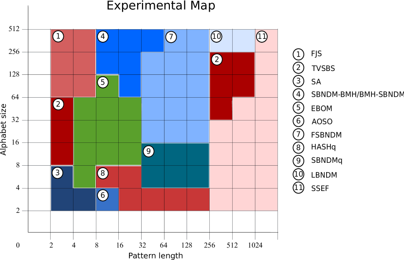
Figure 5: Experimental map of the best results obtained in our evaluation. Comparison based algorithms are presented in red gradations, automata based algorithms are presented in green gradations and bit parallel algorithms are presented in blu gradations.

We performed comparisons between 85 exact string matching algorithms with 12 text of different types. We divide the patterns into four classes according to their length $m$: very short ($m\leq 4$), short ($4<m\leq 32$), long ($32<m\leq 256$) and very long ($m>256$). We proceed in the same way for the alphabet according to their size $\sigma$: very small ($\sigma<4$), small ($4\leq\sigma<32$), large ($32\leq\sigma<128$) and very large ($\sigma>128$). According to our experimental results, we conclude that the following algorithms are the most efficient in the following situations (see Figure 5):

• SA: very short patterns and very small alphabets.

• TVSBS: very short patterns and small alphabets, and long patterns and large alphabets.

• FJS: very short patterns and large and very large alphabets.

• EBOM: short patterns and large and very large alphabets.

• SBNDM-BMH and BMH-SBNDM: short patterns and very large alphabets.

• HASH$q$: short and large patterns and small alphabets.

• FSBNDM: long patterns and large and very larghe alphabets.

• SBNDMq: long pattern and small alphabets.

• LBNDM: very long patterns and very large alphabets.

• SSEF: very long patterns.

Among these algorithms all but one (the SA algorithm) have been designed during the last decade, four of them are based on comparison of characters, one of them is based on automata (the EBOM algorithm) while six of them are bit-parallel algorithms.

References

- [AC91] A. Apostolico and M. Crochemore. Optimal canonization of all substrings of a string. Inf. Comput., 95(1):76–95, 1991.
- [ACR99] C. Allauzen, M. Crochemore, and M. Raffinot. Factor oracle: a new structure for pattern matching. In J. Pavelka, G. Tel, and M. Bartosek, editors, SOFSEM’99, Theory and Practice of Informatics, number 1725 in Lecture Notes in Computer Science, pages 291–306, Milovy, Czech Republic, 1999. Springer-Verlag, Berlin.
- [AG86] A. Apostolico and R. Giancarlo. The Boyer-Moore-Galil string searching strategies revisited. SIAM J. Comput., 15(1):98–105, 1986.
- [AKC03] M. Ahmed, M. Kaykobad, and R. A. Chowdhury. A new string matching algorithm. Int. J. Comput. Math., 80(7):825–834, 2003.
- [AR00] C. Allauzen and M. Raffinot. Simple optimal string matching algorithm. J. Algorithms, 36(1):102–116, 2000.
- [BBE+83] A. Blumer, J. Blumer, A. Ehrenfeucht, D. Haussler, and R. McConnel. Linear size finite automata for the set of all subwords of a word: an outline of results. Bull. Eur. Assoc. Theor. Comput. Sci., 21:12–20, 1983.
- [BBE+85] A. Blumer, J. Blumer, A. Ehrenfeucht, D. Haussler, M. T. Chen, and J. Seiferas. The smallest automaton recognizing the subwords of a text. Theor. Comput. Sci., 40(1):31–55, 1985.
- [BM77] R. S. Boyer and J. S. Moore. A fast string searching algorithm. Commun. ACM, 20(10):762–772, 1977.
- [BR99] T. Berry and S. Ravindran. A fast string matching algorithm and experimental results. In J. Holub and M. Šimánek, editors, Proceedings of the Prague Stringology Club Workshop ’99, pages 16–28, Czech Technical University, Prague, Czech Republic, 1999. Collaborative Report DC–99–05.
- [BYG92] R. Baeza-Yates and G. H. Gonnet. A new approach to text searching. Commun. ACM, 35(10):74–82, 1992.
- [BYR92] R. A. Baeza-Yates and M. Régnier. Average running time of the Boyer-Moore-Horspool algorithm. Theor. Comput. Sci., 92(1):19–31, 1992.
- [CCG+94] M. Crochemore, A. Czumaj, L. Ga̧sieniec, S. Jarominek, T. Lecroq, W. Plandowski, and W. Rytter. Speeding up two string matching algorithms. Algorithmica, 12(4/5):247–267, 1994.
- [CF03] D. Cantone and S. Faro. Fast-Search: a new efficient variant of the Boyer-Moore string matching algorithm. In WEA 2003, volume 2647 of Lecture Notes in Computer Science, pages 247–267. Springer-Verlag, Berlin, 2003.
- [CF04] D. Cantone and S. Faro. Searching for a substring with constant extra-space complexity. In P. Ferragina and R. Grossi, editors, Proc. of Third International Conference on Fun with algorithms, pages 118–131, 2004.
- [CF05] D. Cantone and S. Faro. Fast-Search Algorithms: New Efficient Variants of the Boyer-Moore Pattern-Matching Algorithm. J. Autom. Lang. Comb., 10(5/6):589–608, 2005.
- [CFG10a] D. Cantone, S. Faro, and E. Giaquinta. Bit-(parallelism)2: Getting to the next level of parallelism. In Paolo Boldi and Luisa Gargano, editors, Fun with Algorithms, volume 6099 of Lecture Notes in Computer Science, pages 166–177. Springer-Verlag, Berlin, 2010.
- [CFG10b] D. Cantone, S. Faro, and E. Giaquinta. A compact representation of nondeterministic (suffix) automata for the bit-parallel approach. In A. Amir and L. Parida, editors, Combinatorial Pattern Matching, volume 6129 of Lecture Notes in Computer Science, pages 288–298. Springer-Verlag, Berlin, 2010.
- [CL08] M. Crochemore and T. Lecroq. A fast implementation of the Boyer-Moore string matching algorithm. manuscript, 2008.
- [CLP98] C. Charras, T. Lecroq, and J.D. Pehoushek. A very fast string matching algorithm for small alphabets and long patterns. In M. Farach-Colton, editor, Proceedings of the 9th Annual Symposium on Combinatorial Pattern Matching, number 1448 in Lecture Notes in Computer Science, pages 55–64, Piscataway, NJ, 1998. Springer-Verlag, Berlin.
- [CLRS01] T. H. Cormen, C. E. Leiserson, R. L. Rivest, and C. Stein. Introduction to Algorithms. MIT Press, second edition, 2001.
- [Col91] L. Colussi. Correctness and efficiency of the pattern matching algorithms. Inf. Comput., 95(2):225–251, 1991.
- [Col94] L. Colussi. Fastest pattern matching in strings. J. Algorithms, 16(2):163–189, 1994.
- [CP91] M. Crochemore and D. Perrin. Two-way string-matching. J. Assoc. Comput. Mach., 38(3):651–675, 1991.
- [CR94] M. Crochemore and W. Rytter. Text algorithms. Oxford University Press, 1994.
- [Cro85] M. Crochemore. Optimal factor transducers. In A. Apostolico and Z. Galil, editors, Combinatorial Algorithms on Words, volume 12 of NATO Advanced Science Institutes, Series F, pages 31–44. Springer-Verlag, Berlin, 1985.
- [Cro92] M. Crochemore. String-matching on ordered alphabets. Theor. Comput. Sci., 92(1):33–47, 1992.
- [DC09] S. Deusdado and P. Carvalho. GRASPm: an efficient algorithm for exact pattern-matching in genomic sequences. Int. J. Bioinformatics Res. Appl., 5(4):385–401, 2009.
- [DHPT09] B. Durian, J. Holub, H. Peltola, and J. Tarhio. Tuning BNDM with q-grams. In I. Finocchi and J. Hershberger, editors, Proceedings of the Workshop on Algorithm Engineering and Experiments, ALENEX 2009, pages 29–37, New York, New York, USA, 2009. SIAM.
- [FG05] K. Fredriksson and S. Grabowski. Practical and optimal string matching. In M. P. Consens and G. Navarro, editors, SPIRE, volume 3772 of Lecture Notes in Computer Science, pages 376–387. Springer-Verlag, Berlin, 2005.
- [FJS07] F. Franek, C. G. Jennings, and W. F. Smyth. A simple fast hybrid pattern-matching algorithm. J. Discret. Algorithms, 5(4):682–695, 2007.
- [FL08] S. Faro and T. Lecroq. Efficient variants of the Backward-Oracle-Matching algorithm. In Jan Holub and Jan Žďárek, editors, Proceedings of the Prague Stringology Conference 2008, pages 146–160, Czech Technical University in Prague, Czech Republic, 2008.
- [Fre09] K. Fredriksson. Succinct backward-DAWG-matching. J. Exp. Algorithmics, 13:1.8–1.26, 2009.
- [FYM09] H. Fan, N. Yao, and H. Ma. Fast variants of the backward-oracle-marching algorithm. In Proceedings of the 2009 Fourth International Conference on Internet Computing for Science and Engineering, ICICSE ’09, pages 56–59, Washington, DC, USA, 2009. IEEE Computer Society.
- [GG92] Z. Galil and R. Giancarlo. On the exact complexity of string matching: upper bounds. SIAM J. Comput., 21(3):407–437, 1992.
- [GS83] Z. Galil and J. Seiferas. Time-space optimal string matching. J. Comput. Syst. Sci., 26(3):280–294, 1983.
- [HAKS+08] A. Hudaib, R. Al-Khalid, D. Suleiman, M. Itriq, and A. Al-Anani. A fast pattern matching algorithm with two sliding windows (TSW). J. Comput. Sci., 4(5):393–401, 2008.
- [Han93] C. Hancart. Analyse exacte et en moyenne d’algorithmes de recherche d’un motif dans un texte. Thèse de doctorat, Université Paris 7, 1993.
- [HD05] J. Holub and B. Durian. Talk: Fast variants of bit parallel approach to suffix automata. In The Second Haifa Annual International Stringology Research Workshop of the Israeli Science Foundation, http://www.cri.haifa.ac.il/events/2005/string/presentations/Holub.pdf, 2005.
- [HFS05] L. He, B. Fang, and J. Sui. The wide window string matching algorithm. Theor. Comput. Sci., 332(1-3):391–404, 2005.
- [Hor80] R. N. Horspool. Practical fast searching in strings. Softw. Pract. Exp., 10(6):501–506, 1980.
- [HS91] A. Hume and D. M. Sunday. Fast string searching. Softw. Pract. Exp., 21(11):1221–1248, 1991.
- [KMP77] D. E. Knuth, J. H. Morris, Jr, and V. R. Pratt. Fast pattern matching in strings. SIAM J. Comput., 6(1):323–350, 1977.
- [KPT08] P. Kalsi, H. Peltola, and J. Tarhio. Comparison of exact string matching algorithms for biological sequences. In M. Elloumi, J. Küng, M. Linial, R. F. Murphy, K. Schneider, and C. Toma, editors, Proceedings of the Second International Conference on Bioinformatics Research and Development, BIRD’08, volume 13 of Communications in Computer and Information Science, pages 417–426, Vienna, Austria, 2008. Springer-Verlag, Berlin.
- [KR87] R. M. Karp and M. O. Rabin. Efficient randomized pattern-matching algorithms. IBM J. Res. Dev., 31(2):249–260, 1987.
- [Kül08] M. Oğuzhan Külekci. A method to overcome computer word size limitation in bit-parallel pattern matching. In S.-H. Hong, H. Nagamochi, and T. Fukunaga, editors, Proceedings of the 19th International Symposium on Algorithms and Computation, ISAAC 2008, volume 5369 of Lecture Notes in Computer Science, pages 496–506, Gold Coast, Australia, 2008. Springer-Verlag, Berlin.
- [Kül09] M. Oğuzhan Külekci. Filter based fast matching of long patterns by using simd instructions. In Jan Holub and Jan Žďárek, editors, Proceedings of the Prague Stringology Conference 2009, pages 118–128, Czech Technical University in Prague, Czech Republic, 2009.
- [Lec92] T. Lecroq. A variation on the Boyer-Moore algorithm. Theor. Comput. Sci., 92(1):119–144, 1992.
- [Lec07] T. Lecroq. Fast exact string matching algorithms. Inf. Process. Lett., 102(6):229–235, 2007.
- [LWLL06] C. Liu, Y. Wang, D. Liu, and D. Li. Two improved single pattern matching algorithms. In ICAT Workshops, pages 419–422, Hangzhou, China, 2006. IEEE Computer Society.
- [MP70] J. H. Morris, Jr and V. R. Pratt. A linear pattern-matching algorithm. Report 40, University of California, Berkeley, 1970.
- [Nav01] G. Navarro. NR-grep: a fast and flexible pattern-matching tool. Softw. Pract. Exp., 31(13):1265–1312, 2001.
- [Neb06] M. E. Nebel. Fast string matching by using probabilities: on an optimal mismatch variant of Horspool’s algorithm. Theor. Comput. Sci., 359(1):329–343, 2006.
- [NR98a] G. Navarro and M. Raffinot. A bit-parallel approach to suffix automata: Fast extended string matching. Technical Report TR/DC–98–1, Department of Computer Science, University of Chile, 1998.
- [NR98b] G. Navarro and M. Raffinot. A bit-parallel approach to suffix automata: Fast extended string matching. In M. Farach-Colton, editor, Proceedings of the 9th Annual Symposium on Combinatorial Pattern Matching, number 1448 in Lecture Notes in Computer Science, pages 14–33, Piscataway, NJ, 1998. Springer-Verlag, Berlin.
- [NR00] G. Navarro and M. Raffinot. Fast and flexible string matching by combining bit-parallelism and suffix automata. ACM J. Experimental Algorithmics, 5:4, 2000.
- [PT03] H. Peltola and J. Tarhio. Alternative algorithms for bit-parallel string matching. In M. A. Nascimento, E. Silva de Moura, and A. L. Oliveira, editors, Proceedings of the 10th International Symposium on String Processing and Information Retrieval SPIRE’03, volume 2857 of Lecture Notes in Computer Science, pages 80–94, Manaus, Brazil, 2003. Springer-Verlag, Berlin.
- [Rai92] T. Raita. Tuning the Boyer-Moore-Horspool string searching algorithm. Softw. Pract. Exp., 22(10):879–884, 1992.
- [SAP+04] S.S. Sheik, S.K. Aggarwal, A. Poddar, N. Balakrishnan, and K. Sekar. A fast pattern matching algorithm. J. Chem. Inf. Comput., 44:1251–1256, 2004.
- [Sim93] I. Simon. String matching algorithms and automata. In R. Baeza-Yates and N. Ziviani, editors, Proceedings of the 1st South American Workshop on String Processing, pages 151–157, Universidade Federal de Minas Gerais, Brazil, 1993.
- [SM07] M.A. Sustik and J.S. Moore. String searching over small alphabets. In Technical Report TR-07-62, Department of Computer Sciences, University of Texas at Austin, 2007.
- [Smi91] P. D. Smith. Experiments with a very fast substring search algorithm. Softw. Pract. Exp., 21(10):1065–1074, 1991.
- [Sun90] D. M. Sunday. A very fast substring search algorithm. Commun. ACM, 33(8):132–142, 1990.
- [TVL+06] R. Thathoo, A. Virmani, S. Sai Lakshmi, N. Balakrishnan, and K. Sekar. TVSBS: A fast exact pattern matching algorithm for biological sequences. J. Indian Acad. Sci., Current Sci., 91(1):47–53, 2006.
- [Yao79] A. C. Yao. The complexity of pattern matching for a random string. SIAM J. Comput., 8(3):368–387, 1979.
- [ZT87] R. F. Zhu and T. Takaoka. On improving the average case of the Boyer-Moore string matching algorithm. J. Inform. Process., 10(3):173–177, 1987.
- [ZZMY09] G. Zhang, E. Zhu, L. Mao, and M. Yin. A bit-parallel exact string matching algorithm for small alphabet. In X. Deng, J. E. Hopcroft, and J. Xue, editors, Proceedings of the Third International Workshop on Frontiers in Algorithmics, FAW 2009, Hefei, China, volume 5598 of Lecture Notes in Computer Science, pages 336–345. Springer-Verlag, Berlin, 2009.