Scalar Moduli, Wall Crossing and Phenomenological Predictions

1 Introduction

The physics of wall crossing [1] has received considerable attention from the perspective of theoretical developments, model building and phenomenological predictions. Various prior supergravity models pertaining to the multiplet structures have been developed in the literature [2]. In this concern, string theory plays a crucial role in bringing out all possible spacetime dimensions in a unified framework [3]. Recently, there have been a number of investigations involving $D$-brane instantons in type-II compactifications [4] $D$-instanton counting [5] and corresponding microscopic properties. The above first consideration leads to the notion of moduli stabilization, while the second one leads to the localization of an arbitrary $p$-form. Hereby, the hypermultiplet structure [6] and the corresponding moduli space geometry play an important role in understanding the phenomenon of wall crossing, duality symmetries and twistor space properties. Various algebraic properties of the wall crossing phenomenon opens up a new avenue to learn modern issues of background scalar fields, viz., $(2,2)$ superconformal theories, $D$-terms, quasihomogeneous superpotentials and spectral flow properties [7].

In sequel, black hole physics has revealed an understanding of $AdS_{5}\times S^{5}$ geometry [8] and the corresponding microscopic aspects of a class of higher derivative corrected black holes [9]. The development does not stop here, but it continues far beyond the expectation, viz. the overall theme of microstate counting, $D$-brane instantons, and wall crossing hints about the structure of the nonperturbative string theory [10]. From the perspective of AdS/CFT correspondence [11], and hidden conformal field theory [12], this offers generalized thermodynamical properties of BPS and non-BPS black holes, Hawking radiation, symmetry breaking and the phenomenology of general black holes in string theory. For the case of the two parameter Hawking radiating black hole configurations [13], the constant amplitude radiation and decreasing amplitude York model demonstrate that the statistical fluctuations pertaining to horizon perturbations, quantum gravity corrections and radiation flux can be globally stabilized in specific frequency channels.

From the perspective of the real intrinsic Riemannian geometry, the interesting cases arise for arbitrary charges of the gauged supergravity and arbitrary component scalar moduli configurations. A priori, we have analyzed the moduli stabilization properties of the singlet and doublet complex scalar fields [14], which correspond to the pure marginal and threshold configurations. Algebraically, the above consideration shows that the BPS walls of moduli stability arise as certain polynomial relations in the Fayet parameter. Here we will describe a much more extensive class of exact, analytic stabilization properties for the $D$-term and $F$-term moduli potentials. The present solutions of intrinsic moduli stabilization have an arbitrary number of scalar fields. Our solution may help to clarify many moduli vacuum stabilization effects, which we have recently introduced for the two and four components real scalar fields. As per the notion of moduli configuration, our proposal may play an important role in the exact phenomenological predictions of the string theory moduli space configurations.

2 Fayet Moduli Configurations

The $D$-term moduli configuration may in general be described by the potential

$$V_{D}(\varphi_{i})=(\sum_{i\in\Lambda}\ q_{i}\ \varphi_{i}^{{\dagger}}\varphi_{i}+b)^{2},$$ (1)

where $b$ is the Fayet term. Here we want to analyze “walls of BPS stabilities” by focusing our attention on the role of the intrinsic Riemannian geometry. In order to keep arbitrary electric charges, we shall consider the configuration in its most general form. It is worth to recall that the marginal stability of the vacuum fluctuations requires uniform sign of the electric charges, which must retain the same sign as the Fayet term. Whilst, the threshold stability requires relative signs of electric charges such that the $D$-term can vanish, in order to satisfy the supersymmetry property of the vacuum. The main purpose of the present article is to illustrate phenomenological properties of the moduli stabilization for such a generic vacuum configuration. Let us first illustrate the stabilization properties of the configurations with fewer constituent moduli scalar fields. For a given complex modulus $\varphi_{i}:=(x_{1},x_{2})\in U(1)$, the marginal stability of the vacuum configuration is described by the following Fayet potential

$$V(x_{1},x_{2}):=(x_{1}^{2}+x_{2}^{2}+b)^{2}.$$ (2)

On the other hand, the corresponding threshold configuration with two real scalar fields requires to consider two complex scalar fields $\{\varphi_{1},\varphi_{2}\}$ in a special way. In order to illustrate the role of the threshold type consideration, let us first focus our attention on the moduli configuration involving only two real scalars. In this case, it turns out that the general vacuum configurations of the present interest can be defined as an element of the moduli space, viz., $\{\varphi_{1},\varphi_{2}\}\in\mathcal{M}_{2}$, such that the $D$-term potential vanishes in the vacuum limit. In fact, it follows that the possible values of the constituent fields are an element of $\mathcal{M}_{2}$, which in the limit of extreme values of the fields, can be defined as the following set

$$\mathcal{M}_{2} := \{\{(x_{1},0),(x_{2},0)\},\{(x_{1},0),(0,x_{2})\},$$ (3)

$$\{(0,x_{1}),(x_{2},0)\},\{(0,x_{1}),(0,x_{2})\}\}.$$

In order to ensure supersymmetry, we are required to choose two alternating abelian charges, which in an appropriate normalization correspond to the choice of $q_{1}=1$ and $q_{2}=-1$. Hereby, the threshold stability of the $D$-term moduli configurations pertains to the following Fayet like potential

$$V(x_{1},x_{2}):=(x_{1}^{2}-x_{2}^{2}+b)^{2}.$$ (4)

The two modulus $\{\varphi_{1},\varphi_{2}\}$ case involves four constituent real scalar fields $(x_{1},x_{2},x_{3},x_{4})$. In this case, the $D$-term potential, which corresponds to the marginal moduli configuration, can be expressed as

$$V(x_{1},x_{2},x_{3},x_{4}):=(x_{1}^{2}+x_{2}^{2}+x_{3}^{2}+x_{4}^{2}+b)^{2}.$$ (5)

Correspondingly, the $D$-term potential pertaining to the four constituent real scalar fields, $x_{a}=(x_{1},x_{2},x_{3},x_{4})$, which describes the underlying threshold moduli configuration, takes the following form

$$V(x_{1},x_{2},x_{3},x_{4}):=(x_{1}^{2}+x_{2}^{2}-x_{3}^{2}-x_{4}^{2}+b)^{2}.$$ (6)

In order to appreciate the intrinsic geometric version of the moduli stabilization problem, we may consider a set of real scalar fields $\{x_{i}\}\in\mathcal{M}$ such that the map $V:\mathcal{M}\rightarrow R$ defines the real scalar potential of the complex scalar moduli. Thus, we may geometrically analyze how the transformations $b\mapsto-b$, $b\mapsto 0$ and $b\mapsto 1/b$ appear in the self pair correlation functions and the global correlation volume on the vacuum moduli fluctuations. One of the interesting transformation properties could be to examine how the local and global vacuum correlation(s) behave under the above dilation and translation of the Fayet parameter $b$.

Notice further that the reflection symmetry of the $D$-term potential is required, due to the supersymmetry constraints. Furthermore, the marginal configurations allow the decay of the BPS configurations to non-BPS configurations. However, the corresponding thresholds configurations do not. In particular, we observe that the threshold configurations possess a nontrivial vacuum moduli, for example $\mathcal{M}_{2}$, as mentioned for the extreme limit of the two complex modulus configuration. Practically, the perspective of the intrinsic geometry shows that such a specification of the threshold configurations corresponds to a particular orientation of the vacuum moduli with respect to the line $b=0$, where the supersymmetry is restored.

3 Intrinsic Geometry

We will explore the moduli stabilization properties of the Fayet like configurations for an arbitrary number of constituent scalar fields. In general, let us first note that the consideration of fractional charges and associated constituent gauge fields motivates us to keep the charges to a set of general real values.

3.1 $F$ Term Fluctuations

To test the properties of our model, let us determine the local and global intrinsic geometric properties corresponding to the $F$-term potential. For given dilaton $\phi$ and axion $a$, the $F$-term potential takes the form $V(x_{1},x_{2})=(x_{1}-x_{2})^{2}$, where the $x_{1},x_{2}$ are functions of $\{\phi,a\}$. For the supersymmetry breaking configurations with $b\neq 0$ and arbitrarily charged dilaton axion like configurations, the moduli space potential can be cascaded as

$$V(x_{1},x_{2}) = (q_{1}x_{1}^{2}+q_{2}x_{2}^{2}+b)^{2},$$ (7)

where $q_{1},q_{2}$ are the abelian charges corresponding to the constituent scalar fields $\{x_{1},x_{2}\}$. In this case, we find that the components of the metric tensor satisfy the following quadratic polynomial relations

$$g_{x_{1}x_{1}} = 12q_{1}^{2}x_{1}^{2}+4q_{1}q_{2}x_{2}^{2}+4q_{1}b,$$

$$g_{x_{1}x_{2}} = 8q_{1}q_{2}x_{1}x_{2},$$

$$g_{x_{2}x_{2}} = 4q_{1}q_{2}x_{1}^{2}+12q_{2}^{2}x_{2}^{2}+4q_{2}b.$$ (8)

From the perspective of the intrinsic geometry, we see that the principle components of the intrinsic metric tensor are symmetric quadratic polynomials in the real scalars, whereas the off-diagonal component is a symmetric quadratic monomial. Hereby, an analogous analysis may as well be performed easily for the concerned global stability of the configuration. In particular, we see that the determinant of the metric tensor takes a well-defined positive-definite quadratic polynomial form

$$\|g\|=16q_{1}q_{2}(q_{1}x_{1}^{2}+q_{2}x_{2}^{2}+b)(b+3q_{2}x_{2}^{2}+3q_{1}x_{1}^{2}).$$ (9)

From the definition of the Gaussian fluctuations, we find that the underlying vacuum moduli configuration has the following invariant scalar curvature

$$R = -b\frac{q_{1}x_{1}^{2}+q_{2}x_{2}^{2}}{(q_{1}x_{1}^{2}+q_{2}x_{2}^{2}+b)^{2}(b+3q_{2}x_{2}^{2}+3q_{1}x_{1}^{2})^{2}}.$$ (10)

For a set of given charges, we see that the scalar curvature vanishes, for the vanishing value of the Fayet parameter. In this case, the determinant of the metric tensor remains a nonzero constant, for the vanishing value of the Fayet parameter. The present investigation demonstrates that the $F$ term scalar moduli configurations are statistically interacting, as long as the vacuum possesses a nonzero Fayet parameter and both the vacuum expectation values, viz., $\{x_{1},x_{2}\}$, do not vanish simultaneously. For all values of the Fayet parameter, it is interesting to notice that the threshold configurations, which are defined as a pair of scalar fields with alternating abelian charges, correspond to a noninteracting statistical basis, whenever the constituent scalar moduli fields take an equal absolute value in the vacuum.

3.2 $D$ Term Fluctuations

Let us now consider a realistic case of the vacuum moduli fluctuation. For arbitrary abelian charges $\{q_{1},q_{2},q_{3},q_{4}\}$, a general complex doublet, when the underlying theory has been broken to the $U(1)\times U(1)$, involves the following Fayet potential

$$V(x_{1},x_{2},x_{3},x_{4}) = (\sum_{i=1}^{4}q_{i}x_{i}^{2}+b)^{2}.$$ (11)

Herewith, we observe that the local moduli pair correlations reduce to the following expressions

$$g_{x_{i}x_{i}} = 12q_{i}x_{i}^{2}+4q_{i}\sum_{j\neq i}q_{j}x_{j}^{2}+4q_{i}b,\ i=1,2,3,4$$

$$g_{x_{i}x_{j}} = 8q_{i}q_{j}x_{i}x_{j},\ \forall i\neq j,\ i,j=1,2,3,4.$$ (12)

As mentioned before, in this case, we find further that the principle components of the metric tensor are polynomials in the scalar fields, while, the off-diagonal terms are monomials in the concerned scalar fields. In order to analyze the internal stability of the configuration, we need to examine the positivity of the principle minors of the metric tensor. In this case, we find that the planar and hyper planar minors are given by the following polynomials

$$g_{2} = 16q_{1}q_{2}(\sum_{i=1}^{4}q_{i}x_{i}^{2}+b)(b+3\sum_{i=1}^{2}q_{i}x_{i}^{2}+\sum_{i=3}^{4}q_{i}x_{i}^{2}),$$

$$g_{3} = 64q_{1}q_{2}q_{3}(\sum_{i=1}^{4}q_{i}x_{i}^{2}+b)^{2}(b+3\sum_{i=1}^{3}q_{i}x_{i}^{2}+q_{4}x_{4}^{2}).$$ (13)

The pattern of the polynomial invariance continues and the corresponding determinant of the metric tensor satisfies the following polynomial expression

$$\|g\| = 256q_{1}q_{2}q_{3}q_{4}(\sum_{i=1}^{4}q_{i}x_{i}^{2}+b)^{3}(3\sum_{i=1}^{4}q_{i}x_{i}^{2}+b).$$ (14)

An analogous analysis may as well be performed further for the computation of the concerned global intrinsic geometric invariant quantity. In particular, we see that the underlying Ricci scalar of the vacuum moduli fluctuations is given by

$$R = -\frac{9}{2}\frac{\sum_{i=1}^{4}q_{i}x_{i}^{2}}{(3\sum_{i=1}^{4}q_{i}x_{i}^{2}+b)^{2}(\sum_{i=1}^{4}q_{i}x_{i}^{2}+b)}.$$ (15)

In this case, we find that the vacuum moduli configurations, defined by the real scalar fields $\{x_{1},x_{2},x_{3},x_{4}\}$, correspond to an interacting statistical syatem for all values of the Fayet parameter. It is worth mentioning that the statistical interactions continue to persist, even for the case when the Fayet parameter vanishes. Further, the global statistical interactions exist in the limiting marginal moduli system with an equal value of the constituent scalar fields.

This shows a clear cut distinction between the global vacuum statistical interactions of the $F$ term moduli and $D$ term moduli configurations. It is observed that the marginal moduli configurations preserved the nature of intrinsic geometric invariants. Specifically, the determinant of the metric tensor remains positive for nontrivial vacua with a given Fayet parameter. However, the threshold vacua change their statistical behavior by a translation in the vacuum expectation values of the constituent scalar fields. For a set of given abelian charges, we find that the global nature of the two and four real scalar moduli marginal and threshold configurations is characterized as

$$R_{mar}(x_{i})|_{x_{i}=x} \neq 0,\ \ R_{thr}(x)|_{x_{i}=x}=0,i=1,2$$

$$R_{mar}(x_{i})|_{x_{i}=x} \neq 0,\ \ R_{thr}(x_{i})|_{x_{i}=x}\neq 0,i=1,2,3,4.$$ (16)

We have generalized the above computation for the six and higher number of real scalars. In fact, we have obtained the exact expressions for the components of the metric tensor, principle minors, determinant of the metric tensor and the underlying scalar curvature of the fluctuating configurations. As per this evaluation, the global correlation properties of the six moduli configuration are shown in Fig.(1). Under the vacuum fluctuations, the first figure describes the ensemble stability of the vacuum configuration and the second figure describes the corresponding phase space stability of the vacuum moduli configuration.

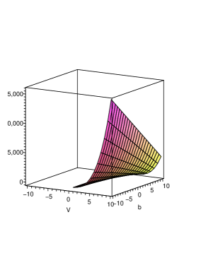
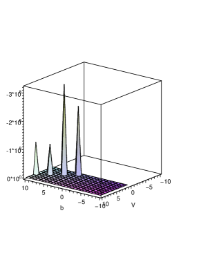
Figure 1: The determinant of the metric and scalar curvature as a function of the potential energy $V$ and Fayet parameter $b$ for the six component real vacuum moduli configuration. As per this prescription, note that we can measure the vacuum fluctuations of an arbitrary finite component scalar moduli configuration.

4 Scalar Phenomenologies

Finally, let us describe the mixing of finitely many real scalar fields. For a set of given abelian charges, the statistical fluctuation of the most general Fayet like configuration involves an ensemble of vacuum moduli fields. As mentioned in the foregoing case, we now consider an extension of the statistical fluctuations pertaining to the phenomenology of the Fayet models, with a set of finitely many constituent real scalar fields. The picture of the marginal and threshold configurations continues to hold for an ensemble of the constituent scalar fields. For $q_{i}\in R$, let $V(\{x_{i}\})=(\sum_{i\in\Lambda}q_{i}x_{i}^{2})^{2},\Lambda\subset Z$ be the Fayet potential. Then, the global vacuum correlation volume, when considered as the scalar curvature of the corresponding statistical configuration, is described as

$$R(\{x_{i}\}=(const).\frac{\sum_{i\in\Lambda}q_{i}x_{i}^{2}}{(b+3\sum_{i\in\Lambda}q_{i}x_{i}^{2})^{2}}\frac{(\tilde{\beta}b+\tilde{\alpha}\sum_{i\in\Lambda}q_{i}x_{i}^{2})}{\|g\|_{linear}},$$ (17)

where $\|g\|_{linear}$ is a $C^{\infty}$ smooth linear map in the $V:\mathcal{M}\rightarrow R$. In this model, we find that the parameters $\{\tilde{\alpha},\tilde{\beta}\}$ can be subsequently determined from the phenomenological considerations of supersymmetry breaking to $U(1)^{r}$. Hereby, we observe that the above claim describes an arbitrary mixing of threshold and marginal configurations, viz., uniform sign of the weight $q_{i}$ for the marginal configurations and alternating sign for the threshold configurations.

Following the foregoing pattern, we find that the $D$ term and $F$ term configurations can completely be determined as a straight line plot between the square root of the Fayet potential and the Fayet parameter. Herewith, from the principle of the mathematical induction, we find further justifications for an increasing number of the constituent scalar fields. In general, let there be $m$ real scalar moduli. Then, as per the pattern observed in the foregoing configurations, we observe that the corresponding intermediate principle minors $p_{n}$ and the determinant of the metric tensor take the following from

$$p_{n} = (\prod_{i=1}^{n}4^{i}q_{i})V(\{x_{i}\})^{\frac{m-1}{2}}(\sqrt{V}+2\sum_{i=1}^{n}q_{i}x_{i}^{2}),$$

$$\|g\| = p_{m}=(\prod_{i=1}^{n}4^{i}q_{i})V(\{x_{i}\})^{\frac{m-1}{2}}(3\sqrt{V}-2b),$$ (18)

where we have taken an account of the fact that arbitrary Fayet potential $V(\{x_{i}\})$ admits a linear combination in the square of the constituent scalar moduli, viz., $\sqrt{V}-b=\sum_{i\in\Lambda}q_{i}x_{i}^{2}$. In this convention, we find the following expression for the scalar curvature

$$R=-(const)\frac{(\sqrt{V}-b)}{V(3\sqrt{V}-2b)^{2}}(\alpha\sqrt{V}+\beta b).$$ (19)

Based on the above observation, we conjecture $\forall i\in\Lambda$ that $\alpha,\beta\in Z$. A physical justification is provided as follows. In doing so, we can easily enlist the specific configurations while verifying the above conjecture, and thus a classification of the scalar moduli configurations. In particular, we find that the vacuum statistical fluctuations can be described by specifying the parameters of the underlying scalar moduli configurations, viz., (i) 2 real scalars: $\alpha=0,\beta=1$, (ii) 4 real scalars: $\alpha=1,\beta=0$ and (iii) 6 real scalars: $\alpha=3,\beta=-1$. For the supersymmetric models broken down to $U(1)^{r}$, we hereby find that the lines of the vacuum phase transitions are $V=0$ and $V=4b^{2}/9$. From the perspective of the local and global mixing, we observe further that the global correlation volume, viz. the scalar curvature, of finitely many scalar moduli configurations can be expressed as

$$R=-\frac{const}{\|g\|^{2}}V^{2\gamma}(\sqrt{V}-b)(\alpha\sqrt{V}+\beta b).$$ (20)

This leads to an observation of the fact that the phenomenology of the scalar moduli correlations arises with $\gamma=k-1$ and $m=2k$. In order to experimentally determine the admissible numerical values of the model parameters $\{\alpha,\beta\}$, let us define $\delta:=-(const)\frac{(\sqrt{V}-b)}{V(3\sqrt{V}-2b)^{2}}$. Thus, for a given vacuum scalar curvature $R$, the Fayet potential and the Fayet parameter satisfy the following linear relation

$$\sqrt{V}=-\frac{\beta}{\alpha}b+\frac{R}{\delta\alpha}.$$ (21)

Experimentally, the parameters $\{\alpha,\beta\}$ can be determined from the slope angle $\theta=-tan^{-1}(\frac{\beta}{\alpha})$ and its intercept $c=\frac{R}{\delta\alpha}$ on the $b$-axis. Specifically, we see that the curve of interaction, as per the characterization of the above straight line, passes from the first and third quadrants. Physically, the constant $\{\alpha,\beta\}$ can be fixed by scaling the scalar potential at a different Fayet parameter. In fact, it follows that our consideration involves only the globally invariant determinant of the metric tensor in the globally invariant scalar curvature, and thus only the correlation dimensions of the vacuum moduli. For a well-defined equilibrium configuration, we find that the underlying statistical system becomes noninteracting for the following case of (i) vanishing vacuum expectation values of the constituent scalar fields, (ii) the square root of the sum of vacuum expectation values of the scalar fields becomes equal to the value of the Fayet parameter and (iii) the parameters of vacuum configuration vanish identically, viz., $\alpha=0,\beta=0$. This provides an excitement for phenomenological aspects of the vacuum fluctuations in the $D$ and $F$ scalar moduli configurations.

References

- [1] E. Witten, JHEP 04 (2002) 012; A. Sen, JHEP 0705 (2007) 039; A. Sen, JHEP 07 (2008) 078; A. Mukherjee, S. Mukhi, R. Nigam, Mod. Phys. Lett. A 24 (2009) 1507-1515; D. Gaiotto, G. W. Moore, and A. Neitzke, Commun. Math. Phys. 299 (2010) 163-224; E. Diaconescu, G. W. Moore, arXiv:0706.3193v1 [hep-th]; F. Denef, JHEP 10 (2002) 023; F. Denef, JHEP 08 (2000) 050; D. Joyce, Adv. Math. 217 (2008), no. 1, 125-204; N. Nekrasov, E. Witten, arXiv:1002.0888v2 [hep-th]; N. A. Nekrasov, Adv. Theor. Math. Phys. 7 (2004) 831-864.
- [2] S. Ferrara, A. Gnecchi, A. Marrani, Phys. Rev. D 78 (2008) 065003; R. D’Auria, S. Ferrara, M. Trigiante. Nucl. Phys. B 780 (2007) 28-39; S. Bellucci, S. Ferrara, A. Marrani, A. Yeranyan, Phys. Rev. D 77 (2008) 085027; G. Gibbons, R. Kallosh, B. Kol, Phys. Rev. Lett. 77 (1996) 4992-4995; D. Green, E. Silverstein, D. Starr, Phys. Rev. D 74 (2006); G. Villadoro, F. Zwirner, JHEP 0603 (2006) 087.
- [3] E. Witten, Nucl. Phys. B 443 (1995) 85-126
- [4] R. Blumenhagen, M. Cvetic, S. Kachru, T. Weigand, Ann. Rev. Nucl. Part. Sci. 59 (2009) 269-296; R. Blumenhagen, S. Moster, E. Plauschinn, Phys. Rev. D 78 (2008) 066008.
- [5] N. Seiberg and E. Witten, Nucl. Phys. B 431, (1994) 19; D. Bellisai, F. Fucito, A. Tanzini, G. Travaglino, Phys. Lett. B 480 (2000) 365-372; U. Bruzzo, F. Fucito, J. F. Morales, A. Tanzini, JHEP 0305 (2003) 054; M. Bianchi, F. Fucito, J. F. Morales, JHEP 0908 (2009) 040.
- [6] B. Pioline, Class. Quant. Grav. 23 (2006) S981; M. Gunaydin, A. Neitzke, B. Pioline, A. Waldron, JHEP 0709 (2007) 056; J. Manschot, B. Pioline, A. Sen, arXiv:1011.1258v2 [hep-th].
- [7] S. Cecotti, Nuc. Phys. B 355, 3, 27 (1991), 755-775; S. Cecotti and C. Vafa, Commun. Math. Phys. 158 (1993) 569-644; arXiv:0910.2615v2 [hep-th]; arXiv:1002.3638v1 [hep-th]; J. J. Heckman, C. Vafa, JHEP 0709 (2007) 011.
- [8] S. Bhattacharyya, S. Lahiri, R. Loganayagam, S. Minwalla, JHEP 0809 (2008) 054; S. Bhattacharyya, S. Minwalla, JHEP 0909 (2009) 034; P. Basu, J. Bhattacharya, S. Bhattacharyya, R. Loganayagam, S. Minwalla, V. Umesh, JHEP 1010 (2010) 045; S. Bhattacharyya, S. Minwalla, K. Papadodimas, arXiv:1005.1287v1 [hep-th].
- [9] R. M. Wald, Phys. Rev. D 48 (1993) 3427-3431; R. M. Wald, Living Rev. Rel. 4 (2001) 6; V. Iyer, R. M. Wald, Phys. Rev. D 50 (1994) 846-864; S. E. Gralla, R. M. Wald, Class. Quant. Grav. 25 (2008) 205009; A. Sen, JHEP 0509 (2005) 038; A. Sen, Gen. Rel. Grav. 40 (2008) 2249-2431; A. Sen, Int. J. Mod. Phys. A 24 (2009) 4225-4244; A. Sen, JHEP 08 (2009) 068; S. Murthy and B. Pioline, JHEP 09 (2009) 022; A. Dabholkar, J. Gomes, S. Murthy, A. Sen, arXiv:1009.3226v1 [hep-th].
- [10] A. Castro, D. Grumiller, F. Larsen, R. McNees, JHEP 0811 (2008) 052; E. Gimon, F. Larsen, J. Simon, JHEP 0907 (2009) 052; A. Castro, F. Larsen, JHEP 0912 (2009) 037; M. Cvetic, F. Larsen, JHEP 0909 (2009) 088; A. Castro, C. Keeler, F. Larsen, arXiv:1004.0554v1 [hep-th].
- [11] J. M. Maldacena, Adv. Theor. Math. Phys. 2 (1998) 231-252; O. Aharony, S. S. Gubser, J. M. Maldacena, H. Ooguri, Y. Oz, Phys. Rept. 323 (2000) 183-386; I. R. Klebanov, E. Witten, Nucl. Phys. B 556 (1999) 89-114; E. Silverstein, E. Witten, Nucl. Phys. B 444 (1995) 161-190.
- [12] A. Castro, A. Maloney, A. Strominger, arXiv:1004.0996v1 [hep-th]; M. Guica, A. Strominger, arXiv:1009.5039v1 [hep-th]; M. Guica, T. Hartman, W. Song, A. Strominger, arXiv:0809.4266v1 [hep-th]; T. Hartman, K. Murata, T. Nishioka, A. Strominger, JHEP 0904 (2009) 019; A. Maloney, W.Song, A. Strominger, Phys. Rev. D 81 (2010) 064007; T. Hartman, W. Song, A. Strominger, arXiv:0912.4265v1 [hep-th].
- [13] S. Bellucci, B. N. Tiwari, JHEP 1011 (2010) 030.
- [14] S. Bellucci, B. N. Tiwari, arXiv:1011.3406 [hep-th].