5-dimensional SU(2) lattice gauge theory with $Z_{2}$ orbifolding and its phase structure

Abstract:

In an $SU(2)$ lattice gauge theory with a $Z_{2}$ orbifolded extra dimension, the new symmetry which is called as a stick symmetry is useful in understanding the bulk transition. We discuss the relation with the Fradkin-Shenker’s phase diagram as well. A remnant of the extra dimension is remained as two $U(1)$ gauge symmetries in two 4-dimensional spaces. We also consider more general bulk gauge groups beyond $SU(2)$.

1 Motivations

Besides supersymmetry, there is an attractive scenario called gauge-Higgs unification in which the Higgs field is identified with the extra component of higher dimensional gauge fields[1, 2], and the gauge symmetry in the scenario is caused by the Hosotani mechanism[3, 4]. In the gauge-Higgs unification scenario by extra-dimensional gauge theories, it is possible to introduce a Higgs field from a gauge field component naturally and the field has only selfcouplings originated by the gauge interaction. The potential term is calculable in principle, although it is difficult.

Generally, an orbifolding condition is imposed to reduce the dynamical freedom of an extra-dimensional system but an origin of the symmetry breaking is also generated because the extra-dimensional profile function is strongly constrained due to the condition. Namely, from orbifolding of an extra-dimensional space, it is possible to induce the origin of the electro-weak symmetry breaking. Since any perturbative approach assumes the existence of a trivial vacuum, although a nonperturbative approach to the unification scenario is valuable, the success of its lattice version depends on whether it can describe correctly the properties of the vacuum.

In this talk, we investigate a 5-dimensional $SU(2)$ gauge theory with $S^{1}/Z_{2}$ orbifolding because $S^{1}/Z_{2}$ orbifolding is the simplest way and we follow to some pioneering works for the lattice formulation [5, 6, 7]. The model has a bulk phase transition characterized by the new symmetry instead of the center symmetry. The center symmetry is helpless owing to $Z_{2}$-projection in this case. The newly found symmetry is called as a stick one [8].

A simple method to study the vacuum structure is to study the phase diagram which describes the property of the vacuum based on the investigation of two couplings parameter space. There is a famous work by Fradkin-Shenker [9] about the gauge-Higgs system in 4-dimensional theories. Our analysis on the phase diagram is carried forward comparing with their work. As the result, we find that two $U(1)$ gauge symmetry in two 4-dimensional spaces are essentially different from any original gauge-Higgs system in 4 dimensions.

For phenomenological applications, we extend the stick symmetry and find that it is admissible only for bulk gauge groups which has even-dimensional fundamental or defining representations.

2 Setup and lattice formulation

We shall start with a 5-dimensional lattice setup for a large 4-dimensional space($x_{\mu}$) and a compact $S^{1}$($x_{5}$). Following to the pioneering works [5, 6, 7], $S^{1}\to S^{1}/Z_{2}$ orbifolding is done in the 5th dimension. Although it is natural to take $x_{\mu}=n_{\mu}a$ and $x_{5}=n_{5}a_{5}$, where the feature of $S^{1}$ reflects on the periodic boundary condition along the 5-th coordinate with a size $2L_{5}$, it is not necessary for $a=a_{5}$, i.e. an isotropical lattice. From the smoothness of our 4-dimensional space, $a$ is enforced to be extremely small or infinitesimal but it is enough for $a_{5}$ to be less than the inverse of our standard model energy scale. Our explicit setup follows as the gauge group is $SU(2)$, a compact 5-dimensional space is $S^{1}/Z_{2}$, the size of our 4-dimensional space is $N_{4}^{4}$. Accordingly, an $SU(2)$ link variables is described as

$$U_{N,M},~{}~{}{M=1,\cdots 5},$$ (1)

where $N$ is a 5-dimensional lattice coordinate $N=\{n_{\nu},n_{5}\}$ and $M$ indicates the direction.

After $Z_{2}$ orbifolding($S^{1}/Z_{2}$), in a bulk space($n_{5}=0,\cdots L_{5}$) $SU(2)$ link variables are projected out as follows;

$$U_{\{n_{\nu},n_{5}\},\mu} =gU_{\{n_{\nu},2L_{5}-n_{5}\},\mu}g^{\dagger},$$

$$U_{\{n_{\nu},n_{5}\},5} =gU^{\dagger}_{\{n_{\nu},2L_{5}-n_{5}-1\},5}g^{\dagger},$$ (2)

and for two special points, FP(1):$n_{5}=0$ and FP(2):$n_{5}=L_{5}$, the projections imply

$$U_{\{n_{\nu},0\},\mu}=gU_{\{n_{\nu},0\},\mu}g^{\dagger},~{}~{}~{}~{}U_{\{n_{\nu},L_{5}\},\mu}=gU_{\{n_{\nu},L_{5}\},\mu}g^{\dagger},$$ (3)

where $g=i\sigma_{3}$. It is found that these two 4-dimensional spaces, FP(1) and FP(2) and the associated symmetries have the important meaning later.

From a usual action,

$$S_{S^{1}}=\beta\sum\limits_{P\in M^{4}\times S^{1}}{[1-\frac{1}{2}{\rm{Tr}}\,\,\,U_{P}]},$$ (4)

we obtain our $Z_{2}$ projected action,

$$S_{S^{1}/Z_{2}}=\beta\sum\limits_{P\in bulk}{[1-\frac{1}{2}{\rm{Tr}}\,\,\,U_{P}]}+{\frac{\beta}{2}}\sum\limits_{P\in{\rm FP(1),FP(2)}}{[1-\frac{1}{2}{\rm{Tr}}\,\,\,U_{P}]}.$$ (5)

Here we note the plaquette made of four link variables as $U_{P}$. The second term of (5) is written by only $U(1)$ plaquettes from $Z_{2}$ orbifolding on FP(1) and FP(2) (3).

3 $Z_{2}$ orbifolding and Stick symmetry

For $Z_{2}$ orbifolded theories, a gauge invariant quantity, is called as $Z_{2}$-projected Polyakov loop, is defined as

$$L_{2}(n_{\nu})\equiv{\rm{Tr}}\,\,U_{\{n_{\nu},0\},5}U_{\{n_{\nu},1\},5}\cdots U_{\{n_{\nu},L_{5}-1\},5}\,\,gU_{{}_{\{n_{\nu},L_{5}-1\},5}}^{\dagger}\cdots U_{{}_{\{n_{\nu},1\},5}}^{\dagger}U_{{}_{\{n_{\nu},0\},5}}^{\dagger}g^{\dagger}$$ (6)

where it is noted that every link variable twice appears in this loop. When we apply the usual center symmetry for this loop, this quantity is invariant and this is not suitable for the order parameter of a symmetry breaking. Nevertheless, our theory, (5) has a phase transition for the loop as seen in Fig.1.

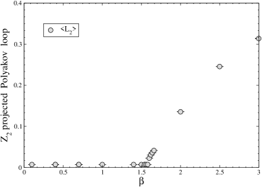
Figure 1: VEV of $Z_{2}$-projected Polyakov loop has been calculated in the lattice system, $N_{4}=8,L_{5}=4$. A small hysteresis effect is observed.

To understand this situation, in our paper[8], we proposed a new symmetry(stick symmetry),

U_{n_ν,L_5},μ → iσ_2 U_{n_ν,L_5},μ( - iσ_2 ) = U^* _{n_ν,L_5},μ , (7)

$$U_{\{n_{\nu},n_{5}\},\mu} \to U_{\{n_{\nu},n_{5}\},\mu}~{}~{}~{}{\rm where}~{}~{}n_{5}=0,\cdots,L_{5}-1,$$

$$U_{\{n_{\nu},n_{5}\},5} \to U_{\{n_{\nu},n_{5}\},5}~{}~{}~{}{\rm where}~{}~{}n_{5}=0,\cdots,L_{5}-2,$$

$$U_{\{n_{\nu},L_{5}-1\},5} \to U_{\{n_{\nu},L_{5}-1\},5}(-i\sigma_{2}).$$

Under the transformation (7), we can show our action (5) and the path integral measure are invariant, $S_{S^{1}/Z_{2}}\to S_{S^{1}/Z_{2}}$ and $~{}~{}dU_{\{n_{\nu},n_{5}\},M}\to dU_{\{n_{\nu},n_{5}\},M}$. Under the stick symmetry, the $Z_{2}$-projected Polyakov loop is transformed as

$$L_{2}(n_{\nu})\to-L_{2}(n_{\nu}),$$ (8)

and the VEV can be an order parameter under the symmetry.

4 Gauge-Higgs system: a comparison with Fradkin-Shenker’s phase diagram

After $Z_{2}$ projected out, the system is equivalent to a $U(1)^{2}$ gauge system, $U(1)|_{\rm FP(1)}$ and $U(1)|_{\rm FP(2)}$ on two 4-dimensional spaces(FP(1),FP(2)) and interacting Higgs fields with them. That is, in the gauge-Higgs unification, the 5-th component of gauge fields corresponds to Higgs fields and it is possible to compare with Fradkin-Shenker’s work[9] for gauge-Higgs systems in 4 dimensions. Short summary for their work about the phase diagram of the gauge coupling $\beta$ and gauge-Higgs coupling $g_{h}$ is listed in the following. For a $U(1)$ gauge plus Higgs system,

• If a Higgs field has a single-unit charge, the phase diagram has no boundary separated between the confinement and the Higgs phases.

• If a Higgs field has other charge such as a double unit charge, the phase diagram may have a boundary separated between the confinement and the Higgs phases.

For a non abelian gauge plus Higgs system,

• If a Higgs field is a fundamental representation, the phase diagram has no boundary separated between the confinement and the Higgs phases.

• If a Higgs field is other representation such as adjoint one, the phase diagram may have a boundary separated between the confinement and the Higgs phases.

The case of no boundary separated between the confinement and the Higgs phases is called as complimentarity. The important point of determining the existence of the phase boundary at $g_{h}\to\infty$ is the vacuum structure of a gauge-Higgs coupling term,

$$g_{h}H^{\dagger}_{n}U_{n,\mu}H_{n+\hat{\mu}}.$$ (9)

When the Higgs field has a single unit charge or belongs to a fundamental representation, the vacuum configuration of the link variable is unique $U_{n,\mu}\sim 1$. When it has a double unit charge or belongs to an adjoint representation, the vacuum configuration is $U_{n,\mu}\sim 1$ or $U_{n,\mu}\sim-1$. On the other hand, in the gauge weak coupling limit $\beta\to\infty$ the vacuum configuration is a unique $U_{n,\mu}\sim 1$. Therefore, in the case of a double unit charge or an adjoint representation, it has a transition point $\beta_{1C}$. Here we must note that it is needless to say the gauge vacuum configuration is gauge-invariant and it is meaningful only to be unique or doubly degenerate. In the addition in the gauge weak coupling limit $\beta\to\infty$, the gauge-Higgs interaction is reduses to the 4-dimensional spin model which has a transition point $g_{hC}$. Two typical cases are drawn in Fig. 2 and Fig. 3.

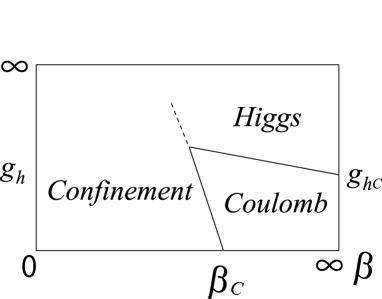
Figure 2: A phase diagram of a gauge field and a fundamental Higgs field system.

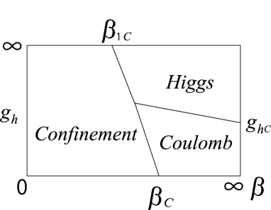
Figure 3: A phase diagram of a gauge field and an adjoint Higgs field system.

When $g_{h}$ goes to infinity, the theory is equivalent to a 4-dimensional spin model coupled to gauge fields with a fixed vacuum angle. The vacuum property depends on the representation or the magnitude of Higgs fields. On the other hand, when $\beta$ goes to infinity, 4-dimensional link variables become trivial and the resulting theory is equivalent to a usual 4-dimensional spin model. Our system is $U(1)\times U(1)$ gauge fields plus a Higgs field. Apparently, this seems to have a Fig.2-type phase diagram because it has no double unit charge. But, the typical interaction between 4-gauge and 5th-gauge fields is

$${\rm Tr~{}}U_{\{n,L_{5}-1\},5}U_{\{n,L_{5}\},\mu}U^{\dagger}_{\{n+\hat{\mu},L_{5}-1\},5}U^{\dagger}_{\{n,L_{5}-1\},\mu},$$ (10)

and the vacuum configuration of the gauge field on the FP(2) is lead to $U_{\{n,L_{5}\},\mu}\sim\pm 1$. Consequently, our system has a similar phase diagram to Fig.3.

Although this discussing model is an effective 4-dimensional gauge-Higgs action, our actual model is a 5-dimensional one. This has so-called a bulk phase transition found by Creutz [10]. The remnant of the 5th dimension in the effective theory is remained as the symmetry $U(1)\times U(1)^{\prime}$. The difference between two U(1) gauge symmetries is characterized by vaious extra-dimensional theories such as matter fields. Based on these results, our model is conjected as Fig.4.

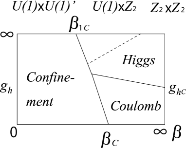
Figure 4:  A phase diagram of a 5-dimensional gauge system with $Z_{2}$ orbifolding. It is expected that the dashed line implies a phase boundary for the breaking of the remained $U(1)$.

Instead of the continuum theory, gauge variant variables in a lattice gauge theories have no physical meaning at all such as profile functions of 5-th components in the bulk gauge fields. Since couplings between FP(2) link variables and 5-th components in link variables on the bulk space are gauge invariant, the Higgs field has a double unit charge coupled to the FP(2) link variables because of non existence of $U(1)|_{\rm FP(2)}$ monopole.

5 Generalization of stick symmetry

We shall consider conditions when there exists the stick symmetry that a bulk gauge symmetry, $G$, breaks into a fixed point gauge symmetry, $H$, where $H=\{h\in G|ghg^{\dagger}=h,g\in G\}$. From the property of $Z_{2}$ orbifolding, $g^{2}$ belongs to the center of $G$, $C(G)$. This means the matrix $g$ which describes $Z_{2}-orbifolding$ can be written as

$$g=\Omega^{1/2}VSV^{\dagger}$$ (11)

where $\Omega$ is an element of C(G), $V$ is a unitary matrix, and $\epsilon$ is defined by $S_{ij}=\epsilon_{i}\delta_{ij}$ with $\epsilon_{i}=\pm 1$. Still, the VEV of $Z_{2}$-projected Polyakov loop must vanish in the strong coupling limit because of the confinement phase,

$$<L_{2}>~{}\propto~{}{\rm{Tr}}~{}g=0.$$ (12)

From (11) and (12), the following condition is lead as

$$\sum_{i}~{}\epsilon_{i}=0,$$ (13)

and it means the irreducible representation belongs to an even dimensional space. If the bulk gauge theory is made of fundamental or defining representations of $SU(2N),SO(2N),F_{4},E_{8},USp(2N)$, its stick symmetry can be realized.

6 Summaries

We consider a lattice $SU(2)$ gauge theory with $S^{1}/Z_{2}$ orbifolding in 5 dimensions. From the numerical simulation, it is guessed that there should exist a certain symmetry in even $S^{1}/Z_{2}$ orbifolding. The new symmetry is called as stick one and corresponds to a kind of a charge conjugation in a fixed point 4-dimensional space, FP(2). Comparing with Fradkin-Shenker’s phase diagram, we can conjecture our theory have one or two phase transition point(s). The first transition is the bulk one by found Creutz firstly [10]. The second transition is originated in a $U(1)$ gauge theory on a 4-dimensional space(FP(2)). If our theory has only a single transition point, it is difficult to take the continuum limit. If our theory has two transition points and a $U(1)$ transition continuously occurs under the confinement phase in the bulk theory, we expect the theory can take the continuum limit.

Phenomenologically, the bulk $SU(2)$ gauge symmetry is too small and we extend the symmetry. Since lattice gauge theories necessarily have a confinement phase in the strong coupling region, the $Z_{2}$-projected Polyakov loop must vanish in the region and it means a stick symmetry unbroken phase. This leads us to a condition; ${\rm Tr~{}}g=0$. If the bulk gauge theory is one of $SU(2N),SO(2N),F_{4},E_{8},USp(2N)$, one shall find its stick symmetry.

References

- [1] C. Csaki, J. Hubisz and P. Meada, TASI Lectures on electroweak symmetry breaking from extra dimensions, [arXiv:hep-ph/0510275].
- [2] H. C. Cheng, Little Higgs, Non-standard Higgs, No Higgs and all that, [arXiv:0710.3407(hep-ph)].
- [3] Y. Hosotani, Dynamical Mass Generation by Compact Extra Dimensions, Phys. Lett. B126 (1983) 309.
- [4] Y. Hosotani, Dynamics of Nonintegrable Phases and Gauge Symmetry Breaking, Ann. Phys. 190 (1989) 233.
- [5] N. Irges and F. Knechtli, Non-perturbative definition of five-dimensional gauge theories on the R orbifold, Nucl. Phys. B719(2005) 121 [hep-lat/0411018].
- [6] N. Irges and F. Knechtli, Non-perturbative mass spectrum of an extra-dimensional orbifold, hep-lat/0604006.
- [7] N. Irges and F. Knechtli, Lattice gauge theory approach to spontaneous symmetry breaking from an extra dimension, Nucl. Phys. B775(2007) 283 [hep-lat/0609045].
- [8] K. Ishiyama, M. Murata, H. So and K. Takenaga, Symmetry and Orbifolding Approach in Five-dimensional Lattice Gauge Theory, Prog. Theor. Phys. 123 (2010) 257 [arXiv:0911.4555].
- [9] E. Fradkin and S. H. Shenker, Phase diagrams of lattice gauge theories with Higgs fields, Phys. Rev. D19 (1979) 3682.
- [10] M. Creutz, Confinement and the Critical Dimensionality of Space-Time, Phys. Rev. Lett. 43 (1979) 553.