Pion mass dependence of the $K_{l3}$ semileptonic scalar form factor within finite volume K. Ghorbani^a,d, M. M. Yazdanpanah^b,d and A. Mirjalili^c,d

a) Physics Department, Faculty of Sciences, Arak University, Arak 38156-8-8349, Iran
b) Physics Department, Kerman Shahid Bahonar University, Kerman, Iran
c) Physics Department, Yazd University, 89195- 741, Yazd, Iran
d) School of Particles and Accelerators, IPM(Institute for research in fundamental sciences), P.O.Box 19395-5531, Tehran, Iran

We calculate the scalar semileptonic kaon decay in finite volume at the momentum transfer $t_{m}=(m_{K}-m_{\pi})^{2}$, using chiral perturbation theory. At first we obtain the hadronic matrix element to be calculated in finite volume. We then evaluate the finite size effects for two volumes with $L=1.83~{}fm$ and $L=2.73~{}fm$ and find that the difference between the finite volume corrections of the two volumes are larger than the difference as quoted in [18]. It appears then that the pion masses used for the scalar form factor in ChPT are large which result in large finite volume corrections. If appropriate values for pion mass are used, we believe that the finite size effects estimated in this paper can be useful for Lattice data to extrapolate at large lattice size.

PACS: 11.15.Ha, 12.39.Fe, 13.20.Eb, 14.40.Aq.

1 Introduction

A precise determination of the CKM matrix element, $V_{us}$, is highly demanded if one expects to find a footprint of new physics in the unitarity relation of the first row of the CKM matrix [1, 2], namely,

$$|V_{ud}|^{2}+|V_{us}|^{2}+|V_{ub}|^{2}=1.$$ (1)

Among three entities above, $|V_{us}|$ is less precisely known from experimental measurements in strangeness changing weak kaon decays $K_{l3}$ and therefore dominates the uncertainty in the unitarity relation. The theoretical framework for the determination of this quantity is explained by Leutwyler and Roos in [3]. To achieve a more precise value of $|V_{us}|$, one requires a better control over the long distance effects due to the strong interactions in the process under consideration. In fact one can only obtain experimentally, the combination $|V_{us}f_{+}(0)|$ by measuring the semileptonic kaon decay rates. Here, $f_{+}(0)$ denotes the related vector form factor at zero momentum transfer. This can be exemplified in the master formula for $K_{l3}$, see [4] and references therein

$$\Gamma\left(K^{i}\to\pi^{j}\ell^{+}\nu_{l}\right)=C^{ij^{2}}\frac{G_{F}^{2}S_{EW}m_{K}^{5}}{192\pi^{3}}\left|V_{us}f_{+}^{K^{i}\pi^{j}(0)}\right|{\cal I}^{ij}_{\ell}\left(1+2\Delta_{EM}^{ij}\right)\,,$$ (2)

where $G_{F}$ is the fermi constant, $S_{EW}$ incorporates the short distance electroweak corrections and ${\cal I}^{ij}_{\ell}$ is the phase-space integral depending on the slope and curvature of the form factors. $f_{+}(0)$ contains the non-perturbative effects of strong interactions whose precision estimate may lower the uncertainties on $|V_{us}|$. There exist two main approaches for the calculation of the vector form factors. One powerful technique is the application of chiral perturbation theory (ChPT) as an effective field theory describing low energy strong interactions. The determination of $f_{+}(0)$ at one loop order within ChPT was evaluated by Gasser and Leutwyler [5]. Along the same lines the calculations were extended further to incorporate two loop order corrections [6]. Despite its model-independent prediction, however, ChPT calculations may become less predictive at higher orders due to undetermined parameters.

Lattice QCD on the other hand, is a brute force approach to determine the QCD observables by evaluating the functional integral of QCD numerically. In recent years the technical procedures have reached to a point that calculations with relatively small quark masses are feasible, see [7, 8, 9, 10, 11] and references therein. Lattice data are not free from systematic errors e.g. finite volume effects and chiral extrapolation. As soon as pion mass is small enough and lattice size is large enough in order to make legitimate application of ChPT for the extrapolations, one can get reliable predictions out of Lattice QCD data. There are a large amount of works in the literature on exploiting ChPT to correct the systematic errors. Lattice size effects on pion mass are studied in [12] and for pion decay constant in [13, 14]. Along the same arguments this type of calculations are done for quark vacuum expectation values [15]. Moreover, finite volume effects on pion pion scattering parameters are evaluated near threshold [16]. There exist Lattice data on the semileptonic vector and scalar form factors, see for example [17, 18, 19, 20, 21]. As suggested in [17, 22] the starting point in doing these calculations in the Lattice is to obtain the scalar form factor at the maximum momentum transfer $t_{m}=(m_{K}-m_{\pi})^{2}$, where high statistical accuracy is achievable. We then deem interesting to evaluate the finite size effects for the scalar semileptonic kaon decay. This decay gives the important key role in kaon physics. Therefore we set the main motivation of the present work as pushing the line of the ChPT applications to a case which involves external momentum. For the sake of simplicity we assume external momentum takes on zero spatial component. To this end, we have checked how far we can get on extending the reliability of ChPT to doing chiral and finite volume extrapolations. Earlier work on finite volume calculations for meson current matrix element with external spatial momentum can be found in [23].

The outline of this article is as follows. We begin with an introduction about ChPT in finite volume and infinite volume in Sec. 2. On Sec. 3 the definition of the $K_{l3}$ form factors are reviewed and in Sec. 4 one loop result of the hadronic matrix element in infinite volume and in a tensor form is provided. Finite volume calculations entailing necessary Feynman integrals in finite volume are sketched in Sec. 5. The last section reports on the finite size effects on the scalar form factor and ends with conclusion.

2 ChPT in infinite and finite volume

2.1 ChPT in infinite volume

Chiral perturbation theory (ChPT) is an effective field theory which describes the low energy dynamics of Quantum Chromo Dynamics (QCD). Weinberg in a seminal paper for the first time paved the way for a systematic application of effective Lagrangian [24]. Pseudo-Goldston mesons play the role of dynamical degrees of freedom in the effective Lagrangian. These mesons are resulted as a consequence of the spontaneous breakdown of the chiral symmetry in QCD. The expansion parameter is generically in terms of the momentum, $p^{2}$, and quark mass, $m_{q}$. Later on Gasser and Leutwyler in two elegant papers extended the Lagrangian to order $p^{4}$ [25, 26]. One can arrange the full effective Lagrangian as series of operators with increasing number of derivatives and increasing power of quark mass

$$\mathcal{L}_{eff}=\mathcal{L}_{2}+\mathcal{L}_{4}+\mathcal{L}_{6}+\cdots\,.$$ (3)

Here the subscripts show the chiral order. The lowest order Lagrangian involving two terms has the following form

$$\mathcal{L}_{2}=\frac{F_{0}^{2}}{4}\left(\langle D_{\mu}UD^{\mu}U^{\dagger}\rangle+\langle\chi U^{\dagger}+U\chi^{\dagger}\rangle\right).$$ (4)

The mass relation $m_{\pi}^{2}=B_{0}\left(m_{u}+m_{d}\right)$ allows one to count quark masses as order $p^{2}$. The next to leading order Lagrangian consists of 10+2 independent operators with corresponding effective low energy constants (LEC’s)

$$\mathcal{L}_{4} =L_{1}\langle D_{\mu}U^{\dagger}D^{\mu}U\rangle^{2}+L_{2}\langle D_{\mu}U^{\dagger}D_{\nu}U\rangle\langle D^{\mu}U^{\dagger}D^{\nu}U\rangle$$ (5)

$$+L_{3}\langle D^{\mu}U^{\dagger}D_{\mu}UD^{\nu}U^{\dagger}D_{\nu}U\rangle$$

$$+L_{4}\langle D^{\mu}U^{\dagger}D_{\mu}U\rangle\langle\chi^{\dagger}U+\chi U^{\dagger}\rangle$$

$$+L_{5}\langle D^{\mu}U^{\dagger}D_{\mu}U(\chi^{\dagger}U+U^{\dagger}\chi)\rangle+L_{6}\langle\chi^{\dagger}U+\chi U^{\dagger}\rangle^{2}$$

$$+L_{7}\langle\chi^{\dagger}U-\chi U^{\dagger}\rangle^{2}+L_{8}\langle\chi^{\dagger}U\chi^{\dagger}U+\chi U^{\dagger}\chi U^{\dagger}\rangle$$

$$-iL_{9}\langle F^{R}_{\mu\nu}D^{\mu}UD^{\nu}U^{\dagger}+F^{L}_{\mu\nu}D^{\mu}U^{\dagger}D^{\nu}U\rangle$$

$$+L_{10}\langle U^{\dagger}F^{R}_{\mu\nu}UF^{L\mu\nu}\rangle+H_{1}\langle F^{R}_{\mu\nu}F^{R\mu\nu}+F^{L}_{\mu\nu}F^{L\mu\nu}\rangle$$

$$+H_{2}\langle\chi^{\dagger}\chi\rangle\,.$$

The notation $\langle...\rangle$ = $\mathrm{Tr}_{F}\left(...\right)$ indicates the trace over the flavors. The matrix $U\in SU(3)$ parameterizes the eight light mesons in an exponential representation

$$U(\phi)=\exp(i\sqrt{2}\phi/F_{0})\,,$$ (6)

where

$$\phi(x)=\,\left(\begin{array}[]{ccc}\displaystyle\frac{\pi_{3}}{\sqrt{2}}\,+\,\frac{\eta_{8}}{\sqrt{6}}&\pi^{+}&K^{+}\\ \pi^{-}&\displaystyle-\frac{\pi_{3}}{\sqrt{2}}\,+\,\frac{\eta_{8}}{\sqrt{6}}&K^{0}\\ K^{-}&\bar{K}^{0}&\displaystyle-\frac{2\,\eta_{8}}{\sqrt{6}}\end{array}\right).$$ (10)

The covariant derivative and the field strength tensor are defined as

$$D_{\mu}U=\partial_{\mu}U-ir_{\mu}U+iUl_{\mu}\,,\quad F_{\mu\nu}^{L}=\partial_{\mu}l_{\nu}-\partial_{\nu}l_{\mu}-i\left[l_{\mu},l_{\nu}\right]\,,$$ (11)

and a similar definition apply to the right-handed field strength. Here $l_{\mu}$ and $r_{\mu}$ represent the left-handed and right-handed chiral currents respectively. $\chi$ is parameterized in terms of scalar ($s$) and pseudo scalar ($p$) external densities as $\chi=2B_{0}\left(s+ip\right)$. For the process discussed in this article it is sufficient to set

$$s=\left(\begin{array}[]{ccc}\displaystyle\hat{m}&&\\ &\displaystyle\hat{m}&\\ &&\displaystyle m_{s}\end{array}\right)\,,l_{\mu}=\frac{g_{2}}{\sqrt{2}}\left(\begin{array}[]{ccc}\displaystyle\hfil&V_{ud}W_{\mu}^{+}&V_{us}W_{\mu}^{+}\\ V_{ud}^{\ast}W_{\mu}^{-}&&\\ V_{us}^{\ast}W_{\mu}^{-}&&\end{array}\right),$$

$$r_{\mu}=0.$$

The weak coupling constant, $g_{2}$, is related to the Fermi constant by

$$\frac{g_{2}^{2}}{8m_{W}^{2}}=\frac{G_{F}}{\sqrt{2}}.$$ (20)

2.2 ChPT in finite volume

The effective Lagrangian approach is also applicable to a system which is bound to a large space of volume $V=L^{3}$ with an infinite time extent. The effective Lagrangian to be used for a system enclosed into a finite size is the same as one we use for processes which occur in infinite volume with the same values for the low energy effective constants. The pioneering works [27, 28, 29] provide the foundations in this regards. To do the calculations in finite volume as suggested in [29] one imposes a periodic boundary condition on particle fields which results in the momentum quantization and consequently the modifications of the quantum corrections. The propagation of a particle in space-time is defined through the two-point correlation function. Therefore the correlation function in finite volume becomes

$$G_{V}=\frac{1}{L^{3}}\sum_{\vec{q}}\int\frac{dq^{0}}{2\pi}G(q^{0},\vec{q}),$$ (21)

where the three dimensional momentum takes the discrete values

$$\vec{q}=\frac{2\pi}{L}\vec{n},$$ (22)

with $\vec{n}$ is a three dimensional vector with integral components and $L$ is the linear size of the box. Since the reliability of ChPT is limited to the small momenta, in finite volume this leads to the condition that

$$F_{\pi}L>>1\,,$$ (23)

where $F_{\pi}$ is the pion decay constant. In addition we stay in a limit where the Compton wavelength of the pion is smaller than the lattice size, $L$, so that the zero mode of the pion field does not become strongly coupled. This condition is satisfied if

$$m_{\pi}L>>1\,.$$ (24)

This is the so-called p-regime in which we do our calculations here. Moreover, the quantity $m_{\pi}L$ plays the role of the power counting in the perturbative calculations.

3 The definition of the $K_{l3}$ form factors

The semileptonic kaon weak decays which are generally shown as $K_{l3}$ are:

$$K^{+}(p)\to\pi^{0}(p^{\prime})l^{+}(p_{l})\nu_{l}(p_{\nu})\,,$$ (25)

$$K^{0}(p)\to\pi^{-}(p^{\prime})l^{+}(p_{l})\nu_{l}(p_{\nu}).$$ (26)

Here $l$ stands for $electron$ and $muon$. The two other processes are charge conjugate modes of the processes above.
Neglecting scalar and tensor contributions, the matrix element takes on the structure

$${\cal M}=\frac{G_{F}}{\sqrt{2}}V^{\ast}_{us}J^{\mu}F^{+}_{\mu}(p^{\prime},p),$$ (27)

with

$$J^{\mu} ={\bar{u}}(p_{\nu})\gamma^{\mu}(1-\gamma_{5})v(p_{l}),$$

$$F^{+}_{\mu}(p^{\prime},p) =\hskip 2.84544pt<\pi^{0}(p^{\prime})|{\bar{s}}\gamma_{\mu}u(0)|K^{+}(p)>.$$ (28)

The general form of the vector matrix element is defined

$$<\pi^{0}(p^{\prime})|{\bar{s}}\gamma_{\mu}u(0)|K^{+}(p) =$$

$$\frac{1}{\sqrt{2}}[(p+p^{\prime})_{\mu}f^{K^{+}\pi^{0}}_{+}(t)+(p-p^{\prime})_{\mu}f^{K^{+}\pi^{0}}_{-}(t)].$$

The $K_{l3}$ matrix element for neutral kaon can be obtained when we replace $F^{+}_{\mu}$ by

$$F^{-}_{\mu}(p^{\prime},p) =\hskip 2.84544pt<\pi^{-}(p^{\prime})|{\bar{s}}\gamma_{\mu}u(0)|K^{0}(p)>$$

$$=\frac{1}{\sqrt{2}}[(p+p^{\prime})_{\mu}f^{K^{0}\pi^{-}}_{+}(t)+(p-p^{\prime})_{\mu}f^{K^{0}\pi^{-}}_{-}(t)].$$

The four $K_{l3}$ form factors $f^{K^{+}\pi^{0}}_{\pm}(t)$ and $f^{K^{0}\pi^{-}}_{\pm}(t)$ depend on the four momentum squared which is transferred to the leptons

$$t=(p^{\prime}-p)^{2}=(p_{l}+p_{\nu})^{2}.$$ (31)

In the isospin limit $f^{K^{+}\pi^{0}}_{\pm}(t)=f^{K^{0}\pi^{-}}_{\pm}(t)$. In this article the matrix element in infinite volume is obtained for the neutral koan decay. The scalar form factor which describes the S-wave projection of the matrix element is defined as

$$f_{0}(t)=f_{+}(t)+\frac{t}{m_{K}^{2}-m_{\pi}^{2}}f_{-}(t).$$ (32)

At the point of zero recoil, the general decomposition of the vector current matrix element becomes

$$<\pi^{-}(p^{\prime})|{\bar{s}}\gamma_{\mu}u(0)|K^{0}(p)>_{t_{m}} =$$

$$\frac{1}{\sqrt{2}}[(m_{K}+m_{\pi})f^{K^{0}\pi^{-}}_{+}(t_{m})+(m_{K}-m_{\pi})f^{K^{0}\pi^{-}}_{-}(t_{m})]\delta_{\mu 0}\,,$$

where $t_{m}=(m_{K}-m_{\pi})^{2}$ is the value of momentum transfer at the special point in the kinematical region. Given the definition of the scalar form factor in Eq. (32) and the matrix element in Eq. (3) we find the following relation at the maximum momentum transfer

$$<\pi^{-}(p^{\prime})|{\bar{s}}\gamma_{\mu}u(0)|K^{0}(p)>_{t_{m}}=\frac{m_{K}+m_{\pi}}{\sqrt{2}}f_{0}(t_{m})\delta_{\mu 0}.$$

4 Analytical results in infinite volume

In this section we recalculate the $K_{l3}$ vector form factors at order ${\cal O}(p^{2})$ and ${\cal O}(p^{4})$ in the isospin limit. On top of this, we also obtain a new expression at one loop order for strangeness changing matrix element in a tensor form which is useful for finite volume calculations to be discussed in Sec. 5 and Sec. 6. In the next subsection we introduce the matrix element in its new form and recall the old results. Feynman diagrams up to order $p^{4}$ in chiral order needed for the interested process are provided by Fig. 1.

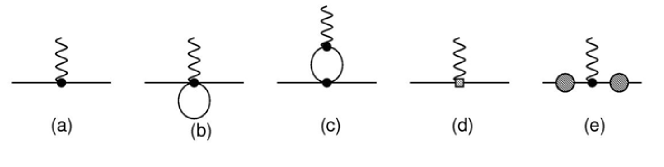
Figure 1: Feynman diagrams contributing to the form factors. Diagram (a) is of ${\cal O}(p^{2})$ with a vertex from the ${\cal O}(p^{2})$ Lagrangian. The rest of the diagrams are of ${\cal O}{(p^{4})}$. Diagram (d) takes its vertex from the ${\cal O}(p^{4})$ Lagrangian and diagram (e) is the wave function corrections to the external legs. The thick lines define meson propagations and wavy lines indicate the gauge boson.

4.1 ${\cal O}(p^{2})$ and ${\cal O}(p^{4})$

In the isospin limit the vector form factors and scalar form factor at leading order are

$$f^{2}_{+}(t)=f^{2}_{0}(t)=1\,, \hskip 14.22636ptf^{2}_{-}(t)=0.$$ (35)

The superscribe indicates the chiral order. These results are obtained by calculating the tree Feynman diagram in Fig. 1(a). At the next order there are four diagrams contributing to the matrix element as depicted in Fig. 1(b-e). Without using the tensor simplification relations for the tensor integrals, we evaluate all the diagrams and sum of the four diagrams read the following expression

$$F(p,p^{\prime}).\epsilon =\frac{1}{F_{\pi}^{2}}\Big{[}2q^{2}L_{9}+[\frac{3}{8}A(m_{\pi}^{2})+\frac{3}{8}A(m_{\eta}^{2})$$ (36)

$$+\frac{3}{4}A(m_{K}^{2})]r.\epsilon-[\frac{3}{2}B_{\mu\nu}(m_{\pi}^{2},m_{K}^{2},q^{2})$$

$$+\frac{3}{2}B_{\mu\nu}(m_{K}^{2},m_{\eta}^{2},q^{2})]r^{\nu}\epsilon^{\mu}+[-2(m_{K}^{2}-m_{\pi}^{2})L_{9}$$

$$+4(m_{K}^{2}-m_{\pi}^{2})L_{5}+\frac{1}{2}A(m_{\eta}^{2})-\frac{5}{12}A(m_{\pi}^{2})$$

$$+\frac{7}{12}A(m_{K}^{2})]q.\epsilon+B(m_{\pi}^{2},m_{K}^{2},q^{2})(\frac{5}{12}q^{2}$$

$$-\frac{5}{12}m_{K}^{2}-\frac{1}{12}m_{\pi}^{2})q.\epsilon+B(m_{K}^{2},m_{\eta}^{2},q^{2})(\frac{1}{4}q^{2}$$

$$-\frac{7}{12}m_{K}^{2}+\frac{1}{12}m_{\pi}^{2})q.\epsilon-[\frac{5}{6}B_{\mu\nu}(m_{\pi}^{2},m_{K}^{2},q^{2})$$

$$+\frac{1}{2}B_{\mu\nu}(m_{K}^{2},m_{\eta}^{2},q^{2})]q^{\mu}\epsilon^{\nu}+B_{\mu}(m_{\pi}^{2},m_{K}^{2},q^{2})\times$$

$$[\frac{3}{4}(p+p^{\prime})^{\mu}q.\epsilon+\frac{5}{12}q^{\mu}q.\epsilon+\frac{5}{6}m_{K}^{2}\epsilon^{\mu}+\frac{1}{6}m_{\pi}^{2}\epsilon^{\mu}$$

$$-\frac{5}{6}q^{2}\epsilon^{\mu}]+B_{\mu}(m_{K}^{2},m_{\eta}^{2},q^{2})[\frac{3}{4}(p+p^{\prime})^{\mu}q.\epsilon$$

$$+\frac{1}{4}q^{\mu}q.\epsilon+\frac{7}{6}m_{K}^{2}\epsilon^{\mu}-\frac{1}{6}m_{\pi}^{2}\epsilon^{\mu}-\frac{1}{2}q^{2}\epsilon^{\mu}]\Big{]},$$

with

$$r=p^{\prime}+p\,, \hskip 14.22636ptq=p^{\prime}-p\,,$$ (37)

and $\epsilon$ is the polarization four vector of the gauge boson. The integral functions $A,B,B_{\mu}$ and $B_{\mu\nu}$ are introduced in the Appendix. In infinite volume, it is possible to use the tensor simplification relations which are provided in the Appendix, to reduce the tensor integrals in terms of scalar functions. The one loop integrals can be evaluated by applying the dimensional regularization scheme. The infinities arising from loop integrals can be canceled by redefining (in a renormalization scheme as discussed in [26]) the LEC’s in terms of renormalized LEC’s and subtracted parts containing infinities. After doing the renormalization, we ensure the cancellation of infinities and recover the old results [3]

$$f_{+}^{K^{0}\pi^{-}(4)}(t) =\frac{1}{F_{\pi}^{2}}\Big{[}2\,L^{r}_{9}t+\frac{3}{8}\,\overline{A}(m_{\pi}^{2})+\frac{3}{4}\,\overline{A}(m_{K}^{2})$$ (38)

$$+\frac{3}{8}\,\overline{A}(m_{\eta}^{2})-\frac{3}{2}\,\overline{B}_{22}(m_{\pi}^{2},m_{K}^{2},t)$$

$$-\frac{3}{2}\,\overline{B}_{22}(m_{K}^{2},m_{\eta}^{2},t)\Big{]}\,,$$

$$f_{-}^{K^{0}\pi^{-}(4)}(t) =\frac{1}{F_{\pi}^{2}}\,\Big{[}-2\,m_{K}^{2}\,L^{r}_{9}+4\,m_{K}^{2}\,L^{r}_{5}-4\,m_{\pi}^{2}\,L^{r}_{5}$$ (39)

$$+2\,m_{\pi}^{2}\,L^{r}_{9}-\frac{5}{12}\,\overline{A}(m_{\pi}^{2})+\frac{7}{12}\,\overline{A}(m_{K}^{2})$$

$$+\frac{1}{2}\,\overline{A}(m_{\eta}^{2})+\overline{B}(m_{\pi}^{2},m_{K}^{2},t)\,(\frac{5}{12}\,t-\frac{5}{12}\,m_{K}^{2}$$

$$-\frac{1}{12}\,m_{\pi}^{2})+\overline{B}(m_{K}^{2},m_{\eta}^{2},t)\,(\frac{1}{4}\,t-\frac{7}{12}\,m_{K}^{2}$$

$$+\frac{1}{12}\,m_{\pi}^{2})+\,\overline{B}_{1}(m_{\pi}^{2},m_{K}^{2},t)\,(-\frac{5}{12}\,t+\frac{19}{12}\,m_{K}^{2}$$

$$-\frac{7}{12}\,m_{\pi}^{2})+\,\overline{B}_{1}(m_{K}^{2},m_{\eta}^{2},t)\,(-\frac{1}{4}\,t+\frac{23}{12}\,m_{K}^{2}$$

$$-\frac{11}{12}\,m_{\pi}^{2})+\,\overline{B}_{21}(m_{\pi}^{2},m_{K}^{2},t)\,(-\frac{5}{6}\,t-\frac{3}{2}\,m_{K}^{2}$$

$$+\frac{3}{2}\,m_{\pi}^{2})+\overline{B}_{21}(m_{K}^{2},m_{\eta}^{2},t)\,(-\frac{1}{2}\,t-\frac{3}{2}\,m_{K}^{2}$$

$$+\frac{3}{2}\,m_{\pi}^{2})-\frac{5}{6}\,\overline{B}_{22}(m_{\pi}^{2},m_{K}^{2},t)$$

$$-\frac{1}{2}\,\overline{B}_{22}(m_{K}^{2},m_{\eta}^{2},t)\Big{]}.$$

5 Finite volume calculations

When we enclose a system in a finite box, Lorentz symmetry is no longer respected. This can make it impossible to define without ambiguity vector form factors for such a system. It also turns out impossible to define vector form factors at the point of zero recoil energy in finite volume because it is always possible to reshuffle terms in the matrix element in such a way to obtain different values for $f_{+}$ and $f_{-}$ according to their definitions in Eq.(3). However, we see from Eq.(3) that the time component of the matrix element at the maximum momentum transfer, $t_{m}$, is proportional to the scalar form factor and therefore the evaluation of the time component of the matrix element in finite volume can give us the scalar form factor at $t_{m}$. The one-loop Feynman integrals which contribute to the matrix element of the process are evaluated in this section. We expect finite volume effects arising from the simultaneous propagation of kaon and eta particles to be much smaller than the same effects when pion and kaon propagate simultaneously in the loop. We demonstrate this claim quantitatively in the next subsection.

5.1 Scalar one-loop integrals

We work out in this subsection the one-loop scalar integrals in detail. In what follows we define for a generic function, F, $\Delta F=F_{V}-F_{\infty}$. Subscripts $V$ and $\infty$ indicate integration in finite and infinite volume, respectively. In finite volume, as we mentioned before, momentum $\vec{q}$ gets discrete values, $\vec{q}=\frac{2\pi}{L}\vec{n}$, but we obtain our formula for the case with infinite time extension. We begin with the tadpole integral

$$A_{V}(m) =-\frac{i}{L^{3}}\sum_{\vec{q}}\int\frac{dq_{0}}{2\pi}\frac{1}{q^{2}-m^{2}}$$ (40)

$$=A_{\infty}-i\int\frac{dq_{0}}{2\pi}\sum_{\vec{n}\neq 0}\int\frac{d^{3}\vec{q}}{(2\pi)^{3}}\frac{e^{iL\vec{q}.\vec{n}}}{q^{2}-m^{2}}.$$

To get the second equality we have used the Poisson summation formula

$$\frac{1}{L^{3}}\sum_{\vec{q}=\frac{2\pi}{L}\vec{n}}f(\vec{q}~{}^{2})=\int\frac{d^{3}q}{(2\pi)^{3}}f(\vec{q}~{})+\sum_{\vec{n}\neq 0}\int\frac{d^{3}q}{(2\pi)^{3}}f{(\vec{q}~{})}e^{iL\vec{q}.\vec{n}}.$$ (41)

By evaluating the contour integral over $q_{0}$ in Eq.(40) we arrive at

$$A_{V}(m)=A_{\infty}(m)-\sum_{\vec{n}\neq 0}\int\frac{d^{3}\vec{q}}{(2\pi)^{3}}\frac{e^{iL\vec{q}.\vec{n}}}{2\sqrt{\vec{q}^{2}+m^{2}}}.$$ (42)

We finally take the final integral and obtain

$$\Delta A=-\frac{m}{4\pi^{2}L}\sum_{\vec{n}\neq\vec{0}}\frac{1}{|\vec{n}|}m(k)K_{1}(mL|\vec{n}|),$$ (43)

where function $K_{1}$ is the modified Bessel function of order one. m(k) accounts for the number of ways that the equality $\vec{n}^{2}=n_{1}^{2}+n_{2}^{2}+n_{3}^{2}$ is satisfied for positive and negative integer numbers for $n_{1}$, $n_{2}$ and $n_{3}$. This result agrees with that in [15].

The second Feynman integral we need to consider here, involves the propagation of two particles with different masses. At the momentum transfer, $t_{m}=(M_{K}-M_{\pi})^{2}$, we first perform the integral for particles with masses $M=M_{K}$ and $m=M_{\pi}$ in the propagators

$$B_{V} =-\frac{i}{L^{3}}\sum_{\vec{q}}\int\frac{dq_{0}}{2\pi}\frac{1}{q^{2}-m^{2}}\frac{1}{(q+p)^{2}-M^{2}}=B_{\infty}$$

$$-\int\frac{dq_{0}}{2\pi}\sum_{\vec{n}\neq 0}\int\frac{d^{3}\vec{q}}{(2\pi)^{3}}\frac{ie^{iL\vec{q}.\vec{n}}}{(q^{2}-m^{2})((q+p)^{2}-M^{2})}\,,$$

where the Poisson summation formula is employed to get the second line. For a simplifying assumption we take the external momentum completely in the time direction as $p=(p_{0},\vec{0})$ and we proceed by exploiting the Feynman parameter formula to get

$$B_{V}=B_{\infty}-i\int_{0}^{1}dx\int\frac{dq_{0}}{2\pi}\sum_{\vec{n}\neq 0}\int\frac{d^{3}\vec{q}}{(2\pi)^{3}}\frac{e^{iL\vec{q}.\vec{n}}}{[q^{2}+x(1-x)p_{0}^{2}-xm^{2}-(1-x)M^{2}]^{2}}\,.$$

We first perform a contour integration over $q_{0}$ and then plug in $p_{0}^{2}=t_{m}$ to find

$$B_{V}=B_{\infty}+\frac{1}{4}\sum_{\vec{n}\neq 0}\int\frac{d^{3}\vec{q}}{(2\pi)^{3}}e^{iL\vec{q}.\vec{n}}\int_{0}^{1}\frac{dx}{[\vec{q}^{2}+(xm+(x-1)M)^{2}]^{3/2}}.$$ (46)

Taking the integral over $x$ gives

$$B_{V}=B_{\infty}+\frac{1}{4(M-m)}\sum_{\vec{n}\neq 0}\int\frac{d^{3}\vec{q}}{(2\pi)^{3}}e^{iL\vec{q}.\vec{n}}(\frac{M}{\vec{q}^{2}\sqrt{\vec{q}^{2}+M^{2}}}-\frac{m}{\vec{q}^{2}\sqrt{\vec{q}^{2}+m^{2}}}).$$ (47)

The second piece contains a three dimensional integral where integration over the angular part leaves us with

$$B_{V}=B_{\infty}-\frac{i}{(2\pi)^{2}4(M-m)L}\sum_{\vec{n}\neq 0}\frac{1}{|\vec{n}|}\int_{-\infty}^{+\infty}d|\vec{q}|\hskip 2.84544pt(\frac{Me^{iL|\vec{q}||\vec{n}|}}{|\vec{q}|\sqrt{{|\vec{q}|}^{2}+M^{2}}}-\frac{me^{iL|\vec{q}||\vec{n}|}}{|\vec{q}|\sqrt{{|\vec{q}|}^{2}+m^{2}}}).$$

To carry out the last integration we make use of the convolution technique. After taking the integral we obtain

$$\Delta B=\frac{1}{16\pi(M-m)}\sum_{\vec{n}\neq 0}M[L_{-1}(ML|\vec{n}|)K_{0}(ML|\vec{n}|)+L_{0}(ML|\vec{n}|)K_{1}(ML|\vec{n}|)]$$

$$-m[L_{-1}(mL|\vec{n}|)K_{0}(mL|\vec{n}|)+L_{0}(mL|\vec{n}|)K_{1}(mL|\vec{n}|)].$$

$L_{\alpha}$ and $K_{\alpha}$ are respectively modified Struve and modified Bessel functions of order $\alpha$. In Fig. 2, the function $\Delta B$ is plotted versus $L$ for three different values of the pion mass while we change the kaon mass correspondingly. The results in Fig. 2 show a reasonable trend. In addition, we need to perform another one-loop integral for propagating particles with masses $M_{\eta}$ and $M_{K}$. It turned out that one cannot find a formula in closed form in this case. The final result for the $K-\eta$ loops reads

$$\Delta B=\frac{1}{8\pi^{2}}\sum_{\vec{n}\neq 0}\frac{1}{L|\vec{n}|}\Big{(}\frac{H_{1}+H_{2}}{H_{1}}\int_{0}^{\infty}\frac{Sin(L|\vec{n}|q)qdq}{(\vec{q}^{2}+H_{3})\sqrt{(H_{1}+H_{2})^{2}+H_{3}+\vec{q}^{2}}}$$

$$-\frac{H_{2}}{H_{1}}\int_{0}^{\infty}\frac{Sin(L|\vec{n}|q)qdq}{(\vec{q}^{2}+H_{3})\sqrt{H_{2}^{2}+H_{3}+\vec{q}^{2}}}\Big{)}\,,$$

where

$$H_{1}=M_{K}-M_{\pi}\,,$$ (51)

$$H_{2}=\frac{M_{K}^{2}-M_{\eta}^{2}-(M_{K}-M_{\pi})^{2}}{2(M_{K}-M_{\pi})}\,,$$

$$H_{3}=M_{\eta}^{2}-H_{2}^{2}.$$

We solve the integral above numerically and plot the function $\Delta B$ versus $L$ as depicted in Fig. 3. By comparing the results in Fig. 2 and Fig. 3, we conclude that the $K-\eta$ loops are suppressed with respect to the $\pi-K$ loops.

Figure 2: $\pi$-K loops in finite volume for three different values of the pion mass and kaon mass.

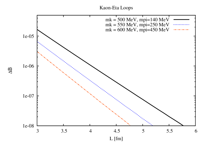
Figure 3: K-$\eta$ loops in finite volume for three different values of the pion mass and kaon mass

5.2 Tensor one-loop integrals

The tensor integral $B^{\mu}$ defined in the Appendix has only one component, i.e. $B^{0}$, needed to be evaluated in the finite volume at the momentum transfer $t_{m}$. We thus consider the integral

$$B_{V}^{0}=-\frac{i}{L^{3}}\int\frac{dq_{0}}{2\pi}\sum_{\vec{q}}\frac{q_{0}}{(q^{2}-m^{2})((q+p)^{2}-M^{2})}=B^{0}_{\infty}+\int\frac{dq_{0}}{2\pi}\sum_{\vec{n}\neq 0}\int\frac{d^{3}\vec{q}}{(2\pi)^{3}}$$ (52)

$$\times\frac{q_{0}\hskip 2.84544pte^{iL\vec{q}.\vec{n}}}{(q^{2}-m^{2})((q+p)^{2}-M^{2})}.$$

The second term which we call $\Delta B^{0}$ can be written in terms of the functions which we obtained already. After doing some manipulations on the integrand, we obtain

$$\Delta B^{0}=\frac{1}{2(M-m)}[\Delta A(m)-\Delta A(M)+2m(M-m)\Delta B].$$ (53)

The last integral we need to calculate in the finite volume is the $B^{00}$ component of the tensor integral $B^{\mu\nu}$. Again we apply the Poisson summation formula to arrive at the second line for the integral below

$$B_{V}^{00} =-\frac{i}{L^{3}}\int\frac{dq_{0}}{2\pi}\sum_{\vec{q}}\frac{q_{0}^{2}}{(q^{2}-m^{2})((q+p)^{2}-M^{2})}$$ (54)

$$=B^{00}_{\infty}-i\int\frac{dq_{0}}{2\pi}\sum_{\vec{n}\neq 0}\int\frac{d^{3}\vec{q}}{(2\pi)^{3}}\frac{q_{0}^{2}\hskip 2.84544pte^{iL\vec{q}.\vec{n}}}{(q^{2}-m^{2})((q+p)^{2}-M^{2})}.$$

We integrate over $q_{0}$ following the same argument sketched before and find

$$\Delta B^{00} =-\int\frac{d^{3}\vec{q}}{(2\pi)^{3}}\frac{e^{iL\vec{q}.\vec{n}}}{2\sqrt{\vec{q}^{2}+M^{2}}}+\frac{1}{4(M-m)}\int\frac{d^{3}\vec{q}}{(2\pi)^{3}}$$ (55)

$$\hskip 17.07182pt\times e^{iL\vec{q}.\vec{n}}(\frac{M(\vec{q}^{2}+m^{2})}{\vec{q}^{2}\sqrt{{\vec{q}}^{2}+M^{2}}}-\frac{m(\vec{q}^{2}+m^{2})}{\vec{q}^{2}\sqrt{{\vec{q}}^{2}+m^{2}}})\,.$$

Substituting the results of Eq.(42) and Eq.(47) into the relation above will yield us

$$\Delta B^{00} =\Delta A(M)-\frac{1}{2(M-m)}[M\Delta A(M)-m\Delta A(m)]+m^{2}\Delta B.$$ (56)

5.3 An asymptotic formula for the scalar form factor

It is important to know the behavior of the finite volume correction of the scalar form factor in asymptotically large volume. To this end, we provide a formula in which we have ignored eta loop effects as well as terms with kaon mass in the exponential and obtain the following result

$$\Delta f_{0}(t_{m}) \simeq\frac{1}{F_{\pi}^{2}}\Big{(}\frac{\sqrt{2m_{\pi}}(m_{K}-19m_{\pi})}{24(2\pi L)^{3/2}(m_{\pi}+m_{K})}$$ (57)

$$+\frac{\frac{34}{27}m_{\pi}^{3}-\frac{5}{12}m_{\pi}^{2}m_{K}+\frac{1}{4}m_{K}^{2}m_{\pi}}{2(\pi L)^{3/2}\sqrt{m_{\pi}}(m_{K}^{2}-m_{\pi}^{2})}\Big{)}\times$$

$$\sum_{\vec{n}\neq 0}\frac{e^{-m_{\pi}L|\vec{n}|}}{{|\vec{n}|}^{3/2}}.$$

Hence, one clearly notices that the volume corrections to the scalar form factor are exponentially suppressed.

6 Numerical results and conclusions

It is seen that the value of the scalar form factor at the endpoint in infinite volume only depends on one low energy constant i.e., $L_{5}^{r}$, which we use as input $L_{5}^{r}=0.97205\times 10^{-3}$, see [30] for detailed discussion on this LEC. The subtraction scale is $\mu=770\,MeV$. There is an ambiguity on the value we should put in for the pion decay constant when one calculates a quantity at one loop order. We use the physical value for the pion decay constant instead of its lowest order value since the difference shifts to higher order. The value $F_{\pi}=0.0924\,GeV$ is chosen as input. The loop integrals in infinite volume are performed with the renormalization scale $\mu=770\,MeV$. We show in Fig. 4 the pion mass dependence of the scalar form factor in infinite volume at the endpoint for $m_{K}=500\,MeV$ and $m_{K}=600\,MeV$. Moreover, from Fig. 4, one can see that in going away from the physical value of the pion mass to an unphysical value of about $350\,MeV$ the scalar form factor in the infinite volume changes about $5$ percent. In addition, we study the volume dependence of the form factor at order $p^{4}$ by defining the ratio

$$R_{f_{0}}=\frac{f_{0}^{V}(t_{m})-f_{0}^{\infty}(t_{m})}{f_{0}^{\infty}(t_{m})}.$$ (58)

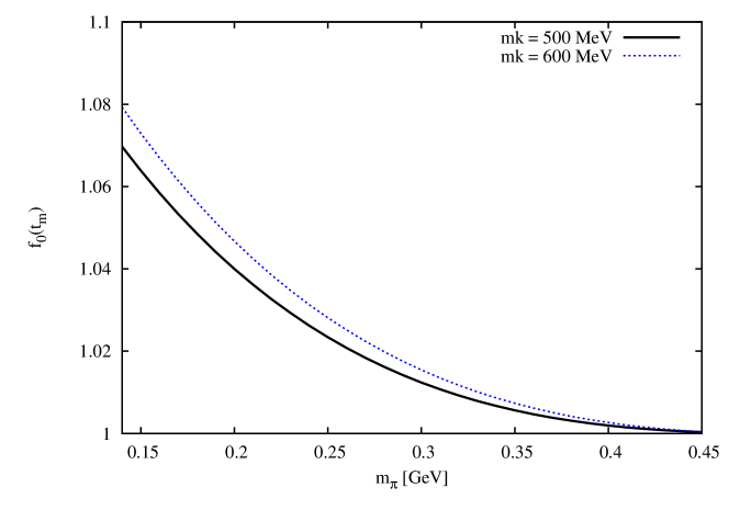
Figure 4: We compare the pion mass dependence of the scalar form factor at the endpoint in the infinite volume for two different values of the kaon mass.

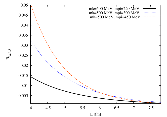
Figure 5: The ratio $R_{f_{0}}$ is plotted versus the linear size of the lattice for pion masses $m_{\pi}=220\,MeV$, $m_{\pi}=300\,MeV$ and $m_{\pi}=450\,MeV$ for a fixed value of the kaon mass, $m_{K}=500\,MeV$.

The ratio $R_{f_{0}}$ is plotted in Fig. 5 versus lattice size, L, for three different values of the pion mass, i.e. $m_{\pi}=220\,MeV$, $m_{\pi}=300\,MeV$ and $m_{\pi}=450\,MeV$, with a fixed value for the kaon mass, $m_{K}=500\,MeV$. The results in Fig. 5 clearly show that for lattice sizes smaller than $L=6.15\,fm$ there is a larger finite size effects for the larger pion mass while the ratio behaves differently for the lattice sizes larger than $L=6.15\,fm$. We found out that the term with the function $B^{0}$ in our finite volume expression for the scalar form factor, takes responsibility for finite volume effects to become large for larger pion mass at small volumes. The reason is that the function $B^{0}$ in the finite volume does not converge fast enough to compensate the quadratic growth of the pion mass in front of $B^{0}$. However, as we see from Eq. 57, the finite volume corrections to the scalar form factor exhibit a standard behavior at asymptotically large pion mass, wherein the corrections suppress exponentially. We therefore stress that the finite volume effects for the scalar form factor at the endpoint can be sizable for $L=4\,fm$ for large pion mass of about $300\,MeV$.

$m_{\pi}(GeV)$	$m_{K}(GeV)$	$m_{\pi}$L	$\Delta f_{0}$ (Only $\pi-K$ loops)	$\Delta f_{0}$ (Including $K-\eta$ loops)	$f^{V}_{0}$	$f^{V}_{0}$ [18]
0.329	0.575	4.50	0.08459	0.08490	1.09532	1.02143(132)
0.416	0.604	5.69	0.11169	0.11196	1.11360	1.00887(89)
0.556	0.663	7.61	0.12323	0.12340	1.12179	1.00192(34)
0.671	0.719	9.19	0.11435	0.11446	1.11382	1.00029(6)

Table 1: We compare our finding for the scalar form factor in finite volume with those quoted in [18], corresponding to the pion masses and kaon masses given in the first and second column. The linear size of the lattice in these calculations is 2.74 fm. Finite volume corrections to the scalar form factor without and with K-$\eta$ loop contributions are given in the forth and fifth column respectively.

In Table 1. we present the finite volume corrections to the scalar form factor and the value of the form factor in finite volume with $L=2.73\,fm$ for particular values of the pion mass and kaon mass as used in [18]. Given the systematic errors in the scalar form factor quoted in [18] our results in Table. 1 show that the lattice data is precise enough for heavier pion masses to take into account the $\eta$ contributions at finite volume. However, our results for the finite volume correction to the scalar form factor at finite volume appear to be large so that the resulting scalar form factor in finite volume is larger than those quoted in [18] while for light pion masses the discrepancy becomes smaller. This is expected from Fig. 5, since our calculated finite volume corrections become large for large pion masses while being in the p-regime, and therefore this is the question of how much SU(3) ChPT is reliable for larger pion masses in the process studied in this article. Moreover, we have also evaluated the finite size effects for a smaller lattice size with $L=1.83\,fm$ and find that the finite volume effects here is about 40 percent which exceed the almost 10 percent finite volume corrections obtained for a lattice with $L=2.73\,fm$. The difference between the estimated finite size effects from ChPT for $L=2.73\,fm$ and $L=1.83\,fm$ is quite larger than the amount of difference as quoted in Table III found in [18]. This is again due to the fact the used pion masses in our ChPT calculations for the scalar form factor are large.

Further work in this direction is to extend our results to non-vanishing spatial momentum since lattice practitioners use these values to interpolate to zero momentum transfer. Moreover, our study can be extended to the case of twisted boundary condition.

7 Appendix

We introduce the one loop Feynman integrals as follows

$$A(m^{2})=\frac{1}{i}\int\frac{d^{d}q}{(2\pi)^{d}}\frac{1}{q^{2}-m^{2}},$$ (59)

$$B(m^{2},M^{2},p^{2}) =\frac{1}{i}\int\frac{d^{d}q}{(2\pi)^{d}}$$ (60)

$$\hskip 14.22636pt\times\frac{1}{(q^{2}-m^{2})((q+p)^{2}-M^{2})},$$

$$B_{\mu}(m^{2},M^{2},p^{2}) =\frac{1}{i}\int\frac{d^{d}q}{(2\pi)^{d}}$$ (61)

$$\hskip 14.22636pt\times\frac{p_{\mu}}{(q^{2}-m^{2})((q+p)^{2}-M^{2})},$$

$$B_{\mu\nu}(m^{2},M^{2},p^{2}) =\frac{1}{i}\int\frac{d^{d}q}{(2\pi)^{d}}$$ (62)

$$\hskip 14.22636pt\times\frac{p_{\mu}p_{\nu}}{(q^{2}-m^{2})((q+p)^{2}-M^{2})}.$$

Invoking lorentz symmetry, the tensor integrals above can be written in terms of scalar functions

$$B_{\mu}(m^{2},M^{2},p^{2})=p_{\mu}B_{1}(m^{2},M^{2},p^{2}),$$ (63)

$$B_{\mu\nu}(m^{2},M^{2},p^{2}) =p_{\mu}p_{\nu}B_{12}(m^{2},M^{2},p^{2})$$ (64)

$$+g_{\mu\nu}B_{22}(m^{2},M^{2},p^{2}).$$

References

- [1] N. Cabibbo, Phys. Rev. Lett. 10 (1963) 531.
- [2] M. Kobayashi and T. Maskawa, Prog. Theor. Phys. 49 (1973) 652.
- [3] H. Leutwyler and M. Roos, Z. Phys. C 25 (1984) 91.
- [4] V. Cirigliano, PoS KAON (2008) 007.
- [5] J. Gasser and H. Leutwyler, Nucl. Phys. B 250 (1985) 517.
- [6] J. Bijnens and P. Talavera, Nucl. Phys. B 669 (2003) 341.
- [7] A. Bazavov et al. [MILC Collaboration], PoS C D09 (2009) 007 [arXiv:0910.2966 [hep-ph]],
- [8] S. Aoki et al. [PACS-CS Collaboration], Phys. Rev. D 79, 034503 (2009),[arXiv:0807.1661 [hep-lat]].
- [9] S. Aoki et al. [PACS-CS Collaboration], Phys. Rev. D 81, 074503 (2010),[arXiv:0911.2561 [hep-lat]].
- [10] S. Durr, Z. Fodor, J. Frison, C. Hoelbling, R. Hoffmann, et al., Science 322, 1224 (2008), [arXiv:0906.3599 [hep-lat]].
- [11] S. Durr, Z. Fodor, C. Hoelbling, S. Katz, S. Krieg, et al.(2010), [arXiv:1011.2403 [hep-lat]].
- [12] G. Colangelo and C. Haefeli, Nucl. Phys. B 744 (2006) 14 [arXiv:hep-lat/0602017].
- [13] G. Colangelo, S. Durr and C. Haefeli, Nucl. Phys. B 721 (2005) 136 [arXiv:hep-lat/0503014].
- [14] G. Colangelo and C. Haefeli, Phys. Lett. B 590 (2004) 258.
- [15] J. Bijnens and K. Ghorbani, Phys. Lett. B 636 (2006) 51.
- [16] P. F. Bedaque, I. Sato and A. Walker-Loud, Phys. Rev. D 73 (2006) 074501.
- [17] D. Becirevic et al., Nucl. Phys. B 705 (2005) 339.
- [18] P. A. Boyle et al., Phys. Rev. Lett. 100 (2008) 141601.
- [19] P. A. Boyle et al., PoS LAT2007 (2007) 380.
- [20] V. Lubicz, F. Mescia, S. Simula, C. Tarantino, and f. t. E. Collaboration, Phys. Rev. D 80, 111502 (2009), [arXiv:0906.4728 [hep-lat]].
- [21] G. Colangelo, S. Durr, A. Juttner, L. Lellouch, H. Leutwyler, et al.,[arXiv:1011.4408 [hep-lat]].
- [22] S. Hashimoto, A. X. El-Khadra, A. S. Kronfeld, P. B. Mackenzie, S. M. Ryan and J. N. Simone, Phys. Rev. D 61 (1999) 014502.
- [23] T. Bunton, F.-J. Jiang, and B. Tiburzi, Phys. Rev. D 74, 034514 (2006), [arXiv:hep-lat/0607001 [hep-lat]].
- [24] S. Weinberg, Physica A 96 (1979) 327.
- [25] J. Gasser and H. Leutwyler, Annals Phys. 158 (1984) 142.
- [26] J. Gasser and H. Leutwyler, Nucl. Phys. B 250 (1985) 465.
- [27] J. Gasser and H. Leutwyler, Phys. Lett. B 184 (1987) 83.
- [28] J. Gasser and H. Leutwyler, Phys. Lett. B 188 (1987) 477.
- [29] J. Gasser and H. Leutwyler, Nucl. Phys. B 307 (1988) 763.
- [30] G. Amoros, J. Bijnens and P. Talavera, Nucl. Phys. B 602 (2001) 87.