Solar energetic events, the solar-stellar connection, and statistics of extreme space weather

Abstract

Observations of the Sun and of Sun-like stars provide access to different aspects of stellar magnetic activity that, when combined, help us piece together a more comprehensive picture than can be achieved from only the solar or the stellar perspective. Where the Sun provides us with decent spatial resolution of, e.g., magnetic bipoles and the overlying dynamic, hot atmosphere, the ensemble of stars enables us to see rare events on at least some occasions. Where the Sun shows us how flux emergence, dispersal, and disappearance occur in the complex mix of polarities on the surface, only stellar observations can show us the activity of the ancient or future Sun. In this review, I focus on a comparison of statistical properties, from bipolar-region emergence to flare energies, and from heliospheric events to solar energetic particle impacts on Earth. In doing so, I point out some intriguing correspondences as well as areas where our knowledge falls short of reaching unambiguous conclusions on, for example, the most extreme space-weather events that we can expect from the present-day Sun. The difficulties of interpreting stellar coronal light curves in terms of energetic events are illustrated with some examples provided by the SDO, STEREO, and GOES spacecraft.

1 Introduction

Magnetic activity of Sun and Sun-like or “cool” stars results in a rich variety of observable phenomena that range from the asterospheres that surround these stars down to the stellar surfaces and – with rapid advances expected in asteroseismology – below. Many of these phenomena are directly observable on Sun and stars alike, including the outer-atmospheric phenomena of persistent chromospheres and coronae, as well as their perturbations in the form of short-lived light-curve perturbations that are the signature of energetic events. It is on the latter that I focus here.

The proximity of the Sun enables us to see details in the evolving magnetic field and associated atmospheric phenomena that are simply impossible to infer from stellar observations. Small wonder, then, that many of the names for stellar phenomena are taken from the solar dictionary: active regions, spots, flares, eruptions, and even the processes such as differential rotation and meridional advection that are part of the equivalent of the magnetic activity cycle, all the way to the loss of angular momentum associated with the gusty outflow of hot, magnetized plasma. Ensembles of observations taken over periods of years to centuries are revealing the statistical properties of some of these phenomena, even as state-of-the art observatories in space and on the ground are revealing physical processes and the interconnectedness of the global outer atmosphere.

But recent observations of the Sun only provide a very limited view of what its magnetic activity has on offer, for at least two reasons. First, our Sun has a magnetic activity cycle that is relatively long compared to researchers’ careers as well as to the era of advanced technology that has aided us in our observations. Consequently, we can expect even the ’present-day Sun’ to have surprises in store for us that we have not yet observed simply because we have not been looking long enough. Some of these surprises may lie hidden in records such as polar ice sheets, while others lie embedded in rocks from outer space. But the lessons that can be learned from these invaluable and, as yet, under-explored archives are limited by access to these resources, by the limited temporal resolution of such records, and by the long chains of processes that sit between a solar phenomenon like the sunspot cycle or its largest flares and the ’recording physics’ for the archive from which we are attempting to learn about them. In addition to learning about the Sun from such ’geological’ records of its activity, one can also perform an ensemble study of states of infrequent extreme solar activity by looking at a sample of stars like it. This can provide us with a large enough sample of Sun-like stars that we can begin to assess how frequently the Sun may subject us to rare but high-impact events such as dangerous superflares and disruptive geomagnetic storms: although rare, the damage that may be inflicted to our global society and its safety and economy by extreme events is of such a magnitude that in-depth study of their properties and likelihood is prudent.

A second reason why stellar studies are crucial to understanding of solar activity is that only stellar observations allow us to explore what the Sun’s activity has been in the very distant past or what it will be in the very distant future (measured on time scales up to billions of years) by selecting stars of a wide range of ages.

In this review, I discuss a sampling of the results coming out of the study of what has been termed the solar-stellar connection. I focus, in particular, on lessons that we are learning about what could be called ’space climate’, i.e., the characteristic state of activity of a star like the Sun including the fluctuations about the mean in the form of energetic events like flares and coronal mass ejections (CMEs). Consequently, one of the topics selected for this review is a comparison of frequency distributions of bipolar regions, flares, CMEs, and solar energetic particle (SEP) events, the possible relationships between them, and the lessons learned by combining solar and stellar observations in our quest to establish the ’laws’ of astro-magnetohydrodynamics. Another topic is that of light curves, which touches on the need to have pan-chromatic knowledge to guide our interpretation of stellar observations as well as on the long-standing concept of ’sympathetic events’ in stellar magnetic activity.

2 The flux spectrum of bipolar regions

Magnetic flux emerges from the solar interior as flux bundles that shape themselves into bipolar regions. Those regions large enough to contain spots during at least some of their mature, coherent phase, are called active regions. Their emergence frequency for sunspot cycle 22 was found to be characterized by a power-law distribution with an index $-\alpha_{\Phi}=2.0\pm 0.1$ (Harvey & Zwaan 1993; Schrijver & Harvey 1994).

The flux bundles that are too small to contain spots, typically with fluxes below about $10^{20}$ Mx, but larger than about $10^{18}$ Mx, are called ephemeral regions. The flux spectrum of the ephemeral regions appears to smooth transition into that of the active region spectrum. When the frequency distributions for active and ephemeral regions are combined into an approximate power-law distribution, one finds

$$N(\Phi){\rm d}\Phi\propto\Phi^{-\alpha_{\Phi}}{\rm d}\Phi$$ (1)

for $\alpha_{\Phi}=2.69$ (Thornton & Parnell 2011). The difference between the above values of $\alpha_{\Phi}$ indicates that a single power-law is too simple as an approximation, with the flux spectrum somewhat less steep with increasing size. For the purpose of the discussion below, I will take the range as a measure of uncertainty, i.e. $\alpha_{\Phi}=2.3\pm 0.3$.

The active-region spectrum for cycle 22 appeared to be roughly fixed in shape, going up and down by a multiplicative factor over the cycle with a power-law index changing by at most a few tenths of its value (Harvey & Zwaan 1993; Schrijver & Harvey 1994). During the recent cycle minimum (late 2008 and early 2009), active regions were essentially absent for a long time, with the 3-month average sunspot number hovering around an unusually low value of 1.5, down from around 150 during characteristic sunspot maxima. The ephemeral-region population, in contrast, remained essentially unchanged (Schrijver et al. 2010). Hence, the bipolar-region spectrum is likely not a single, time-independent power law. Yet, at least during relatively active phases, on which I shall focus below, this simple approximation appears warranted.

Figure 1.: Sample X-ray lightcurves observed with GOES (top) and EUV signals observed with SDO/AIA in the Fe XVI 335 Å channel (center) and the Fe IX/X 171 Å channel (bottom), for an M5.4 active-region flare (left) and for the eruption of a large filament from a quiet-Sun region (right). The intensities were scaled to a pre-event reference value (at the dashed line). Note that the vertical scale of the center-left panel is 10$\times$ that of the other AIA panels.

Eq. (1) characterizes the frequency of emerging bipoles. In a study of bipolar regions existing on the solar surface during 1996 to 2008, Zhang et al. (2010) find a power law with an index of $\alpha_{\rm exist}\sim 1.63$; its lower (absolute) value than $\alpha_{\Phi}$ in Eq. (1) is caused by the longer life time of larger active regions.

The flux distribution reported on by Zhang et al. (2010) exhibits a marked drop below the power law for fluxes exceeding $\Phi\sim 6\times 10^{23}$ Mx, and they find no regions above $\Phi_{\rm max}\sim 2\times 10^{24}$ Mx. Historically, the largest sunspot group recorded occurred in April of 1946, with a value of 6 milliHemispheres (Taylor 1989); for an estimated field strength of 3 kG, that amounts to a flux in the spot group alone of $\Phi_{\rm spots}\sim 6\times 10^{23}$ Mx. The total flux in this spot group was likely larger, but perhaps within a factor of $2-3$ of that in the spots, and thus of the same order of magnitude as the upper limit to the distribution found by Zhang et al. (2010).

During their mature, coherent phase solar active regions are characterized by a remarkably similar flux density, $\langle B\rangle$ of about $100$ Mx/cm² to $150$ Mx/cm² (Schrijver & Harvey 1994) regardless of region size. This allows us to perform a transformation of the frequency distribution of fluxes to one of total energies in the atmospheric field (to be discussed below), using a simple approximation that the energy $E_{B}$ contained in the bipolar-region field for an active region with size $\ell$ scales as

$$E_{B}\propto\langle B\rangle^{2}\ell^{3}\propto(\langle B\rangle\ell^{2})^{3/2}=\Phi^{3/2}.$$ (2)

Thus, when rewriting Eq. (1) in terms of energies one finds:

$$N(\Phi){\rm d}\Phi=n(E_{B}){{\rm d}\Phi\over{\rm d}E_{B}}{\rm d}E_{B}\propto E_{B}^{-{2\over 3}\alpha_{\Phi}-{1\over 3}}{\rm d}E_{B}\equiv E_{B}^{-\mu}{\rm d}E_{B}=E_{B}^{-1.9\pm 0.2}{\rm d}E_{B}.$$ (3)

For the above value of $\Phi_{\rm max}$, the corresponding energy is $E_{B,{\rm max}}\sim 10^{37}$ ergs.

3 The spectral appearance of flares and eruptions

Solar flares span an astonishing range of energies: from the largest flares, emitting brightly in hard X-rays and even $\gamma$ rays, down to the weakest EUV flares barely detectable against the persistent background glow of the quiet-Sun corona. The fact that flares shift in color from EUV for $\sim 10^{24}$-erg nanoflares to hard X-rays for $\sim 10^{32}$-erg X-class events makes a statistical comparison difficult: small and large flares are generally observed with different instruments, exacerbating the difficulties in estimating total energies in the absence of bolometric observables (solar flares are too faint to be picked up by total irradiance monitors, with very few exceptions). This is compounded by problems in estimating the strong background in the case of the weakest events. For the largest flares, there are statistical limitations owing to their low frequency.

The launch of the Solar Dynamics Observatory (SDO) in the spring of 2010 has opened a window onto the global Sun that enables a direct comparison of solar and stellar observations in terms of light curves and their interpretation. The Atmospheric Imaging Assembly (AIA; Lemen et al. 2010) on SDO is a full-disk EUV imaging telescope array that provides high-resolution ($\sim 1.4$ arcsec), high-cadence ($\sim 12$ s) coronal images in 7 narrow-band spectral windows (in addition to a few UV channels). SDO’s Extreme-ultraviolet Variability Experiment (EVE) measures the X-ray and EUV spectral irradiance (e.g., Woods et al. 2010). The comparison of the data from these two instruments is just starting, but already some unanticipated findings are emerging.

One of these surprises has to do with the relationship between flares and CMEs. With the Sun in a moderately active state through much of 2010, SDO has thus far observed primarily C-class flares and only a few low M-class flares. Woods et al. (2010) note that the AIA observations show that about 80% of the C-class flares are associated with CMEs. Earlier work had suggested numbers as low as $\sim 20$% for C-class flares, increasing to $\sim 40$% and $\sim 100$% for M- and X-class flares, respectively (see summary and references in Schrijver 2009). The reason for the relatively large fraction of eruptive events remains subject to investigation; it may reflect a selection bias in earlier studies, or may suggest that flaring during low-activity states more readily breaks through the relatively weak overlying field than during higher activity states.

On another front, even the Sun still has surprises in store as to how flares show themselves in different pass bands. Associated with the large fraction of eruptive C-class flares is a characteristic signature seen in the EVE spectral irradiance measurements: Woods et al. (2010) point out that these eruptive flares have late-phase emissions in, e.g., Fe XV and Fe XVI that AIA data show to be associated with relatively high post-eruption loop systems, apparently reconnecting and cooling after the eruptive flare. That late-phase emission was not observed for C-class solar flares until now.

Another example of what we are learning about solar energetic events is shown in Fig. 1. The top-left panel shows the GOES $0.5-4.0$ Å (lower curve) and $1.0-8.0$ Å (upper curve) signals for the 2010/11/05 M5.4 flare. The AIA lightcurves below it are for the Fe XVI 335 Å and Fe IX/X 171 Å channels. This eruptive flare shows a spike in the Fe XVI 335 Å channel followed by a long-duration signal indicative of the cooling of post-eruption loops (as discussed above for the less energetic C-class flares). The much cooler Fe IX/X 171 Å signal shows a mixture of brightenings and darkenings that reflect heating, cooling, and expansion-related coronal dimmings. For an analogous discussion on stellar flaring, see, e.g., Osten & Brown (1999).

Figure 2.: Sample lightcurves observed with GOES (top) and with SDO/AIA in the Fe XVI 335 Å channel (center) and the Fe IX/X 171 Å channel (bottom), for a series of related coronal mass ejections and flares (as discussed by Schrijver & Title 2010). The intensities were scaled to the time of minimum brightness in the 335 Å channel (at the dashed line). Vertical dashed lines show approximate times of the start of filament eruptions seen in AIA’s 304 Å channel, and dotted lines show when the first signs of CMEs were seen in STEREO’s COR1 images.

The right-hand panels in Fig. 1 show the signals in these same pass bands associated with the eruption of a large quiet-Sun filament from an otherwise quiet-Sun disk. The X-ray brightening barely registers as a flare, reaching no more than the B2 level. The Fe XVI 335 Å signal shows a long-lived brightening followed by a dimming before the signal recovers to pre-eruption levels some 18 h after the onset, while the Fe IX/X 171 Å signal persists as a brightening associated with quiet-Sun post-eruption arcades for that entire period, starting about an hour after the onset of the B2 flare. The total energy (fluence) associated with this event (estimated from EVE measurements by R. Hock, priv. comm.) is $\sim 2\times 10^{30}$ ergs, i.e. comparable to a low M-class flare, not dissimilar from that shown on the left. Despite the comparable energies involved in these two events, the softness of the spectrum and the duration of this very extended event, spanning a good fraction of a solar radius, lead to an entirely different observational appearance if observed through lightcurves as can be obtained for stars.

4 Local and global influences on eruptions

High-resolution solar instruments typically have a limited field of view, while telemetry constraints on, e.g., the full-Sun X-ray imager on YOHKOH often led observers to down-select regions around a flare site to bring down higher-cadence imaging. From that perspective, it is not surprising that many studies looking for conditions leading to the explosive/eruptive release of magnetic energy focus on the conditions within or nearby an active region. This has led to the recognition of certain patterns in the magnetic field generally associated with flaring regions, in particular neutral lines, often with high shear or high gradients (as summarized, e.g., by Schrijver 2009).

The capabilities of SDO’s AIA, particularly when combined with EUV observations from the two STEREO spacecraft that both approach quadrature relative to the Sun-Earth line, are revealing that long-range interactions play an important part in flares and eruptions in addition to the ’internal conditioning’. Schrijver & Title (2010) discuss one particular set of flares and eruptions in detail, but many more similar connections have been inferred from other observations. They use full-sphere magnetic field maps in combination with the STEREO and SDO observations to show that a series of events on 2010/08/01 are directly connected by magnetic field, in particular by field lines that are part of a web of topological fault zones, i.e., separatrices, separators, and quasi-separatrix layers. These long-range connections span across half a hemisphere, part of which was invisible from Earth, but covered by one of the STEREO spacecraft.

These observations reveal that in many cases, what may look like a single event is instead a complex of simultaneous events, or events that occur in close succession, across a large area of a stellar surface. The solar events of 2010/08/01 are dominated by short active-region flare loops in the X-ray part of the spectrum and by long post-eruption loops over quiet-Sun filaments; the combination of these wavelengths to estimate the properties of the field involved, as one might do if these were stellar observations, would lead to fundamentally erroneous conclusions. This is illustrated by the lightcurves in Fig. 2 (showing the same set of signals as Fig. 1): the flares are identifiable in the GOES X-ray signal (top panel), but already of a substantially different character in the Fe XVI 335 Å passband shown below it. Around 1 MK, in the Fe IX/X 171 Å channel, the flares are absent, while the dimmings are not obviously connected to the filament eruptions. Where multi-wavelength coverage would help interpret stellar observations, separation of the multitude of events on that day using only light curves and then estimating total energies from available limited pass bands is obviously an exercise fraught with large ambiguities and uncertainties. The repercussions on such linked (or “sympathetic’) events on the hotly-debated problem of the causal links between flares and CMEs continue to be studied; we may need to follow Harrison (1996) who acknowledges the complex linkages between these event classes and suggests that we refer to their composites as ’coronal magnetic storms,’ a term equally suitable for the stellar arena (where sympathetic flaring is discussed, e.g., by Osten & Brown 1999).

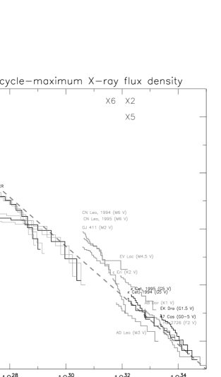
Figure 3.: Downward-cumulative flare frequency distribution for energies exceeding $E$, normalized to approximate solar-maximum X-ray flux density levels ($1.3\times 10^{5}$ erg cm^-2 s^-1; Judge et al. (2003)) assuming a linear dependence of the X-ray surface flux density. Flare spectra for Sun-like G-type stars are shown in black, for warmer and cooler stars in grey. The grey dashed power-law fit has an index of $\alpha_{f}+1=-0.87$. EUV data from Aschwanden (2000), soft X-ray data from Shimizu (1997), hard X-ray data $>8$ keV from Lin et al. (2001), and stellar data from Audard et al. (2000). The grey histograms for solar data bracket a conservative energy uncertainty of a factor of 2. Three estimates of flare energies for GOES X flares are shown near the top, from Aschwanden & Alexander (2001) and Benz (2008).

5 Flare energy spectrum

Despite the difficulties that arise in establishing total energies for the variety of flares even for solar events, the comparison from nanoflares to X-class flares has been made, with the intriguing result that flares span a range of at least 8 orders of magnitude with a frequency distribution that can be approximated by a power-law spectrum.

Statistics on stellar data are even harder to assemble and interpret, but over the years lessons have been learned and numbers extracted. One such study, by Audard et al. (2000), assembles EUVE observations on 10 cool stars into downward-cumulative frequency distributions (to suppress the problem of low-number statistics) of estimated energies. Here, too, power-law spectra arise, in fact with slopes very much like those reported for solar flares. In another study, Wolk et al. (2005) look at young, active stars in the Orion Nebula Cluster, just a few million years old; their flare energy distribution yield a power-law index of $\alpha_{f}\approx 1.7$.

Osten & Brown (1999) – for over 140 d of observations on 16 tidally interacting RS CVn binaries – and Audard et al. (2000) – for some 74 d of observing of 10 single and binary stars – both conclude that the overall flaring rate increases essentially linearly with the background stellar X-ray luminosity, with flares reaching energies of over $10^{34}$ ergs, roughly comparable to a solar X500 flare. If we use the inferred proportionality of flare frequency with X-ray brightness to normalize the observed stellar frequency distribution for flare energies to the Sun characteristic of cycle maximum, the combined solar and stellar flare statistics (Fig. 3, which shows the downward-cumulative frequency distribution) reveals a frequency distribution for flare energies of

$$N(E_{f}){\rm d}E_{f}\propto E_{f}^{-\alpha_{f}}{\rm d}E_{f},$$ (4)

with $\alpha_{f}=-1.87\pm 0.10$ (rough uncertainty estimate). The solar data align remarkably well with those of the G-type main-sequence stars in the sample by Audard et al. (2000).

One property of note here is that the slopes $\alpha_{f}$ in Eq. (4) and $\mu$ in Eq. (3) agree within their uncertainties. What can we infer from this? The scaling of the flare frequency spectra observed for stars is essentially linear with the X-ray brightness of the stars (Audard et al. 2000), which, in turn, is essentially linearly dependent on the unsigned magnetic flux threading the stellar surface (Schrijver 2001), and modeling with a surface flux-transport model suggests that that scales linearly with the rate of emergence of bipolar active regions (Schrijver 2001).

With this chain of linear scalings, it is very tempting to conclude that the flare frequency is proportional to the emergence frequency of bipolar regions. One possible inference from this is that flares draw their power from the same source as the active region magnetic configurations. In that context, it is interesting to note that the flare energy distribution in Fig. 3 does not suggest a cutoff in energy up to values approaching $10^{35}$ ergs, which is comfortably below the maximum available energy $E_{B,{\rm max}}$ estimated above for historically observed solar active regions.

Interestingly, recent Kepler observations of white light flares reported at the 16th workshop on “Cool Stars, Stellar Systems, and the Sun” suggest flares can occur up to at least $10^{37}$ ergs, although these most energetic flares are (at least at present) reported for stars significantly cooler than the Sun, see, e.g., Walkowicz et al. (2010). What does it take to power such large flares? If we assume that a fraction of $f=0.01-0.1$ of the magnetic energy density in a volume with a characteristic mean field strength of $B_{0}$ can be converted into what eventually is radiated from the flare site, the typical dimension $d_{0}$ and magnetic flux $\Phi_{0}=B_{0}d_{0}^{2}$ in such a flaring region are given by

$$d_{0}=\left({4\pi E_{f}/f\over B_{0}^{2}}\right)^{1/3}\,\,;\,\,\Phi_{o}=B_{0}d_{0}^{2}={(4\pi E_{f}/f)^{2/3}\over B_{o}^{1/3}}.$$ (5)

At $B_{0}=300$ G, for flares with $E_{f}=10^{35}$ ergs, $d_{0}\approx(0.7-1.6)R_{\odot}$ and $\Phi_{0}\approx(0.8-4)\,10^{24}$ Mx. Although very sizeable, these numbers are still compatible with the largest fluxes, $\Phi_{\rm max}$, discussed in Sect. 2; note that the value of $B_{0}$ here was chosen 3 times higher than characteristic of solar regions to illustrate how challenging it is to fit the flaring region on the available solar surface (see also, e.g., Osten & Brown 1999, for evidence of extended flaring regions in some RS CVn stars). For $E_{f}=10^{37}$ ergs, on the other hand, $d_{0}\approx(3-7)R_{\odot}$ and $\Phi_{0}\approx(20-80)\,10^{24}$ Mx, which simply would not fit on the Sun, and involves fluxes well above $\Phi_{\rm max}$; conditions for such stellar flares must differ from those on the present-day Sun, and perhaps – as I discuss next – these very extreme events no longer occur on the aged star next door.

6 Spectrum of solar energetic particle events

The frequency distribution in Fig. 3 suggests that if we estimate an X1 flare to have an energy of about $10^{32}$ ergs, we should see about 30 flares per year of that magnitude or larger during active phases in the solar cycle. That number compares quite well with the average frequency of 25 per year for X-class flares over the past three solar cycles, when counting only during the active half of the cycles (see the compilation by Hudson 2007). We would expect an X10 or larger about 4 times per year, which is high by a factor of about three given the 21 observed X-class flares since 1976 with the Sun in an active state for about 15 years within that interval. Extending that spectrum even further, we would expect an X100 flare or larger once every other year for the Sun near cycle maximum. As we have not experienced such large flares in at least half a century, we face the possibility that despite the intriguing alignment of solar and stellar flare data after normalization to the mean coronal brightness, there may in fact be an upper limit to stellar flare energies that may shift to lower values with increasing age even as the spectrum below that value is left unchanged in slope: the solar flare energy distribution appears to drop below the power-law fit in Fig. 3 above X10, and the largest flare observed to date has been estimated to be an X45$\pm 5$ (Thomson et al. 2004).

Are there constraints that can be set on the occurrence of extreme flares that can be found in ’archives’ on Earth other than those compiled by mankind? Solar eruptive events are frequently associated with solar energetic particle (SEP) events that modulate the galactic cosmic ray (GCR) background which itself varies on time scales of years and longer (Schrijver & Siscoe 2010a, b). SEP events can accelerate particles to energies up to several GeV which suffices to initiate a nuclear cascade in the upper layers of the Earth’s atmosphere and in lunar or meteoric rocks. Some constraints on large SEP events can be recovered by studying the mix of radioactive nuclides or in radioactive decay products as a function of penetration depth in lunar and meteoric rock samples, or by studying the so-called odd nitrogen concentrations that are modulated by reactions high in the Earth’s atmosphere that are sensitive to ionization states. The combination of space-age measurements with such geological archival information led Usoskin (2008) to conclude that the downward-cumulative probabilities of large solar proton events scaled with the fluence $F_{\rm p}$ as a power law with a slope of $\delta+1\sim 0.4$ for relatively small events, then turning towards a steeper slope with a lower limit of $\delta+1\leq 0.9$, with the ’break’ occurring around fluences of $10^{10}$ cm^-2 for protons above 10 MeV.

One might deduce from the inferred break in the SEP fluence distribution that the behavior of solar flares changes at high energies. That conclusion is ambiguous based on this argument only, however, as argued by combining several observed frequency distributions. Let us start from the particle fluence distribution

$$N_{\rm p}{\rm d}F_{\rm p}\propto F_{\rm p}^{-\delta}{\rm d}F_{\rm p},$$ (6)

with the above value for $\delta$ as estimated from the cumulative distribution function of the fluences. In order to relate the fluences at Earth to those originating from the solar flares and associated coronal mass ejections (both of which appear to contribute to the SEPs in a mixture that continues to be debated), let us assume that the particles are emitted from their source region in the corona or inner heliosphere into a solid angle that scales with the total energy $E_{\rm f}$ of the eruptive event as

$$\Omega\propto E_{\rm f}^{\gamma}.$$ (7)

The value of $\gamma$ can be estimated by comparing the flare energy distribution in Eq. (4) and the distribution of opening angles, $a$ (in degrees), for eruptions from very large CMEs seen by SOHO’s LASCO to small fibril eruptions observed by TRACE and perhaps for even smaller events seen in STEREO data (summarized by Schrijver 2010)

$$N_{a}{\rm d}a=b\,a^{-\beta}{\rm da},$$ (8)

with $\beta=2.0\pm 0.3$ (estimated from Fig. 2 in Schrijver (2010); $b\approx 1.1$ for $\beta=2$). For given $a$ (in radians), the corresponding fractional solid angle is given by

$${\Omega\over 4\pi}={1\over 2}(1-\cos{a})\approx{1\over 4}a^{2},$$ (9)

where the first term in the Taylor expansion shown on the right approximates the solid angle only for sufficiently small values of $a$, otherwise saturating when the hemisphere above the event is filled at $\Omega=2\pi$. Using the right-hand expression in Eq. (9) together with Eq. (7), we can rewrite Eq. (8) as

$$N_{a}{\rm d}a\propto\Omega^{-{1\over 2}(1+\beta)}{\rm d}\Omega\propto E_{f}^{-{\gamma\over 2}(1+\beta)+\gamma-1}{\rm d}E_{f}.$$ (10)

With Eq. (4), $\alpha_{f}={\gamma\over 2}(1+\beta)-\gamma+1$ one finds $\gamma=2(\alpha_{f}-1)/(\beta-1)$.

Let us further assume that the particle fluence at Earth, $F_{p}$ is a fixed fraction $f$ of $E_{\rm f}$, diluted by expanding over a solid angle $\Omega$, i.e., that with Eq. (7),

$$F_{p}\propto f{E_{\rm f}\over\Omega}\propto E_{\rm f}^{1-\gamma}.$$ (11)

With this, Eq. (6) can be transformed to read

$$N_{\rm p}{\rm d}F_{\rm p}\propto E_{\rm f}^{-\delta(1-\gamma)-\gamma}{\rm d}E_{\rm f}\propto E_{f}^{\rm-\delta+2(\alpha-1)(\delta-1)/(\beta-1)}{\rm d}E_{\rm f}.$$ (12)

The assumption that the SEPs are emitted within a solid angle $\Omega$ implies that only those for which the direction of the Earth (mapped through the curved path of the Parker spiral of the heliospheric magnetic field) is included within that solid angle can be detected (here, I ignore the fact that relatively small flares often do not connect to the heliosphere, see Sect. 3). This means that only a fraction

$$p={\Omega\over 4\pi}\propto E_{\rm f}^{\gamma}$$ (13)

of the total number of events is detected. Hence, to recover the flare energy distribution from the observed SEP fluences, the distribution in Eq. (12) has to be divided by $p$:

$$N_{f}{\rm d}E_{\rm f}\propto E_{\rm f}^{-\delta+2(\alpha-1)(\delta-2)/(\beta-1)}{\rm d}E_{\rm f}\equiv E_{\rm f}^{-\epsilon}{\rm d}E_{\rm f}\stackrel{{\scriptstyle?}}{{=}}E_{\rm f}^{-\alpha_{f}}{\rm d}E_{\rm f}.$$ (14)

With the values of the exponents above, one finds $\epsilon=2.4\pm 0.5$, consistent with the value of $\alpha_{f}$ in the flare energy distribution of Eq. (4) within $\sim 1.1\sigma$, provided we limit the comparison to events for which the SEPs are spread over a solid angle $a$ small compared to $2\pi$ steradians. This slope holds up to an SEP frequency at Earth of about 1/yr; if we assume for those events $\Omega\approx 2\pi$, $p\approx 1/2$, so $\approx 2$/yr for the full Sun; Eq. (8) has that downward cumulative frequency for $a\approx 200^{\circ}$, which is slightly high, but roughly consistent with our hypothetical argumentation. For relatively large opening angles $a$, the expression in Eq. (9) saturates to a constant value, as does the detection probability $p$. In that case, one would expect $\epsilon\approx\delta\approx\alpha$. Such a value is just allowed by the empirical upper limits to the energy distributions from Moon rocks. On the other hand, such a slope may be too shallow relative to what is suggested around the ’break’ in the spectrum from NO₃ data from ice cores as summarized by Usoskin (2008).

From this, we can tentatively conclude that at least the frequency distributions for solar flares, for CME opening angles, and for SEP fluences are consistent for proton events up to the largest observed in the instrumental era. The break in the fluence spectrum above those values might reflect the saturation of the spreading of the SEPs over essentially a full hemisphere over the solar source region. But it is possible that a true saturation occurs somewhere along the chain of events from Sun to Earth: flare energies may have an upper cutoff for the present-day Sun (with flare probabilities dropping significantly below the power-law fit in Fig. 3 for flares above X10) that is not readily inferred by looking at samples of young Suns or the generation of energetic particles may be limited (either at the flare site or within heliospheric shocks).

7 In conclusion

The sample observations discussed above demonstrate that the combination of geophysical, heliophysical, and astrophysical data can teach us much about the Sun’s magnetic climate, up to the most energetic of events. The interpretations outlined are, of course, to be tested and alternatives, that doubtlessly exist, are to be explored. Despite the speculative nature of the scenarios sketched above, it appears that we are close to having the material available to learn where the solar flare-energy spectrum drops below a solar-stellar power law: the combination of the study of archives in ice and of stellar flare statistics should be able to provide us with an answer. On a less positive note, the solar observations discussed above demonstrate that measuring the energies involved in explosive and eruptive events is difficult, that separating events based on lightcurves alone is an ambiguous exercise, and that broad wavelength coverage is essential to both of these objectives: to learn about the most severe space weather, we have to accept that long-duration, large-sample, pan-chromatic (and thus often multi-observatory) stellar observations are needed because they can provide crucial information that can otherwise only be gathered by observing the Sun for a very long time and undergoing the detrimental effects of extreme magnetic storms on the Sun and around the Earth.

Acknowledgments

I thank M. Aschwanden, J. Beer, R. Osten, C. Parnell, and A. Title for discussions, suggestions, and pointers to the literature.

References

- Aschwanden (2000) Aschwanden, M. J. 2000, Solar Phys., 190, 233
- Aschwanden & Alexander (2001) Aschwanden, M. J., & Alexander, D. 2001, Solar Phys., 204, 91
- Audard et al. (2000) Audard, M., Güdel, M., Drake, J. J., & Kashyap, V. L. 2000, ApJ, 541, 396
- Benz (2008) Benz, A. O. 2008, Living Reviews in Solar Physics, 5, 1
- Harrison (1996) Harrison, R. A. 1996, Solar Phys., 166, 441
- Harvey & Zwaan (1993) Harvey, K. L., & Zwaan, C. 1993, Solar Phys., 148, 85
- Hudson (2007) Hudson, H. S. 2007, ApJL, 663, 45.
- Judge et al. (2003) Judge, P. G., Solomon, S. C., & Ayres, T. R., 2003 ApJ, 593, 534.
- Lemen et al. (2010) Lemen, J. R., Title, A. M., Akin, D. J., et al. 2010, submitted to Solar Phys.
- Lin et al. (2001) Lin, R. P., Feffer, P. T., & Schwartz, R. A. 2001, ApJL, 557, L125
- Osten & Brown (1999) Osten, R. A., & Brown, A. 1999, ApJ, 515, 746
- Schrijver & Siscoe (2010a) Schrijver, C., & Siscoe, G. 2010a, Heliophysics. Evolving solar activity and the climates of space and Earth (Cambridge, U.K.: Cambridge University Press)
- Schrijver & Siscoe (2010b) — 2010b, Heliophysics. Space storms and radiation: Causes and Effects (Cambridge, U.K.: Cambridge University Press)
- Schrijver (2001) Schrijver, C. J. 2001, ApJ, 547, 475
- Schrijver (2009) Schrijver, C. J. 2009, Advances in Space Research, 43, 739.
- Schrijver (2010) — 2010, ApJ, 710, 1480.
- Schrijver & Harvey (1994) Schrijver, C. J., & Harvey, K. L. 1994, Solar Phys., 150, 1
- Schrijver et al. (2010) Schrijver, C. J., Livingston, W. C., Woods, T. N., & Mewaldt, R. A. 2010, in preparation.
- Schrijver & Title (2010) Schrijver, C. J., & Title, A. M. 2010, JGR, in press
- Shimizu (1997) Shimizu, T. 1997, in Magnetic Reconnection in the Solar Atmosphere, edited by R. D. Bentley & J. T. Mariska, vol. 111 of Astronomical Society of the Pacific Conference Series, 59
- Taylor (1989) Taylor, P. O. 1989, J. of the American Assoc. of Variable Star Observers, 18, 65
- Thomson et al. (2004) Thomson, N. R., Rodger, C. J., & Dowden, R. L. 2004, Geophys. Res. Lett., 31, 6803
- Thornton & Parnell (2011) Thornton, L. M., & Parnell, C. E. 2011, Solar Phys., in press
- Usoskin (2008) Usoskin, I. G. 2008, Living Reviews in Solar Physics, 5, 3.
- Walkowicz et al. (2010) Walkowicz, L. M., Basri, G., Batalha, N., et al. 2010, ArXiv e-prints 1008.0853
- Wolk et al. (2005) Wolk, S. J., Harnden, F. R., Jr., Flaccomio, E., Micela, G., Favata, F., Shang, H., & Feigelson, E. D. 2005, ApJSS, 160, 423.
- Woods et al. (2010) Woods, T. N., Eparvier, F., Jones, A. R., Hock, R., Chamberlin, P. C., Klimchuk, J. A., Didkovsky, L., Judge, D., Mariska, J., Tobiska, W. K., Schrijver, C. J., & Webb, D. F. 2010
- Zhang et al. (2010) Zhang, J., Wang, Y., & Liu, Y. 2010, ApJ, 723, 1006