Restricting Fourth Order Gravity via Cosmology

Abstract

The cosmology of general fourth order corrections to Einstein gravity is considered, both for a homogeneous and isotropic background and for general tensor perturbations. It is explicitly shown how the standard cosmological history can be (approximately) reproduced and under what condition the evolution of the tensor modes remain (approximately) unchanged. Requiring that the deviations from General Relativity are small during inflation sharpens the current constraints on such corrections terms by some thirty orders of magnitude. Taking a more conservative approach and requiring only that cosmology be approximately that of GR during Big Bang Nucleosynthesis, the constraints are improved by $4\--6$ orders of magnitude.

I Introduction

General Relativity (GR) is often considered to be an extremely well tested physical theory, however compared to the other fundamental constants (e.g. the electron charge, the speed of light etc.), the gravitational constants are rather poorly constrained. Whilst it is true that the predictions of GR have been verified to staggering accuracy (see for example C_Will ), there is little experimental/ observational evidence to restrict corrections of GR that involve higher powers of curvature invariants. This is simply a consequence of the fact that GR has been directly tested in weak curvature regimes, with strong curvature tests (such as near black holes and neutrons stars) typically resulting in theoretical restrictions. The Einstein-Hilbert action for GR contains only terms that are, at most, second order in the derivatives of the metric (in the form of the Ricci scalar $R$) and a natural question to then ask is what restrictions are there on the presence of terms that contain higher order derivatives of the metric?

Motivation for such a question can be found from two, broadly different, approaches. The first is phenomenological: are there corrections to the Einstein-Hilbert action that can better describe observed data? In particular there has been much effort in looking for deviations from GR that might explain the apparent presence of Dark Energy, Dark Matter and inflation (such as $f(R)$ gravity Nojiri:2006ri ; Appleby:2007vb ; Sotiriou:2008rp ; Nojiri:2003ft ; Amendola:2006we ; Nojiri:2008nt ; Nojiri:2010wj ; Capozziello:2007ec ; Capozziello:2006uv ; Nojiri:2007as ; Boehmer:2007kx , chameleon models Khoury:2003aq ; Khoury:2003rn ; Brax:2008hh , conformal gravity Mannheim:1999nc ; Mannheim:1996rv , MOND Milgrom:1992hr ; Milgrom:2002tu ; Bekenstein:2007iq , TeVeS Skordis:2009bf ; Moffat:2005si ; Sagi:2007hb ; Skordis:2005eu ; Sanders:2005vd ; Zlosnik:2006sb etc.). The second approach is to consider theoretically motivated corrections to GR, often due to Quantum Gravity (such as String/ Brane theory Mavromatos:2007sp ; Smolin:1995ai ; Baumann:2009ni ; Brax:2003fv ; Duff:2000mt ; Garriga:1999yh ; Nelson:2008sv ; Germani:2002pt ; Hawking:2000kj ; Kachru:2003sx ; Randall:1999vf ; Sasaki:1999mi , ADS-CFT Anchordoqui:2000du ; Gubser:1999vj ; Nojiri:2000kq , Loop Quantum Gravity Bojowald:2006ww ; lving_rev_MB ; Smolin:2010kk ; Nelson:2007cp ; Bianchi:2009ri ; Bianchi:2006uf ; Smolin:2004sx ; Ashtekar:2004eh ; Thiemann:2007zz ; Baez:1999sr , Chern-Simons theory Alexander:2009tp ; Yunes:2008ua etc.) or a Grand Unification theory (such as Non-commutative Geometry Buck:2010sv ; Chamseddine:2010ud ; Chamseddine:2006ep ). Because there are only three curvature invariants that contain at most two derivatives of the metric, $R$, the cosmological constant $\Lambda$ and the Gauss-Bonnet combination (defined below), one is generally forced to consider correction terms containing $4^{\rm th}$ and higher derivatives of the metric, at least in the low energy, effective limit of the full theory.

Theoretically there is, however, a serious difficultly with a theory that contains higher than second order derivatives of the metric; such a theory would contain ‘ghosts’. These are modes that have a negative kinetic term and can result in super-luminal propagation and other instabilities Barth:1983hb ; Stelle:1977ry ; DeFelice:2006pg . Such difficulties become particularly acute when the theory is quantised, since the presence of ghosts leads to particles with negative energies or states with negative norm. This shows that any theory containing higher order corrections to GR cannot be a fundamental theory unless powerful non-perturbative effects come into play. Here we will consider a general $4^{\rm th}$ order correction to GR and take the point of view that this is an effective theory, approximating (some of) the corrections to GR that are produced by some complete underlying, non-perturbative theory. This precisely is the approach that is taken when renormalisation group techniques are applied to GR Lauscher:2001ya ; Reuter:2001ag ; Donoghue:1993eb .

The only terms containing at most $4^{\rm th}$ order derivatives of the metric that are constructed out of curvature invariants (other than the cosmological constant) are

$$R^{\mu\nu\rho\gamma}R_{\mu\nu\rho\gamma}~{},~{}~{}R^{\mu\nu}R_{\mu\nu}~{},~{}~{}R^{2}~{},~{}~{}R~{},$$ (1)

where $R^{\mu}_{~{}\nu\rho\gamma}$ is the Riemann tensor, defined as

$$R^{\mu}_{~{}\nu\rho\beta}=\Gamma^{\mu}_{\rho\nu,\beta}-\Gamma^{\mu}_{\beta\nu,\rho}+\Gamma^{\alpha}_{\nu\rho}\Gamma^{\mu}_{\beta\alpha}-\Gamma^{\alpha}_{\nu\beta}\Gamma^{\mu}_{\rho\alpha}~{},$$ (2)

and we follow the notation of Nelson:2010ig Greek letters to denote space-time indices; $\Gamma^{\mu}_{\nu\rho}$ is the usual Christoffel symbol; we denote partial derivatives as $\partial_{\eta}R=R_{,0}$ and we use the convention $R_{\mu\nu}=R^{\rho}_{~{}\mu\rho\nu}$, with the signature $\left(-+++\right)$. The Ricci scalar (last term in (1)) is at most second order in derivatives of the metric, while the particular combination, $R^{2}-4R_{\mu\nu}R^{\mu\nu}+R^{\mu\nu\rho\gamma}R_{\mu\nu\rho\gamma}$, called the Gauss-Bonnet combination, satisfies (in four dimensions)

$$\sqrt{-g}\left(R^{2}-4R_{\mu\nu}R^{\mu\nu}+R^{\mu\nu\rho\gamma}R_{\mu\nu\rho\gamma}\right)={\rm total~{}divergence}~{}.$$ (3)

Thus, assuming there are no boundary terms (which can be a significant complication, particularly when attempting to quantise the theory Barth:1983hb ), one can write any $4^{\rm th}$ derivative correction to the Lagrangian of GR as

$${\cal S}=-\int{\rm d}^{4}x\sqrt{-g}\left[\frac{\gamma}{\kappa^{2}}R-\hbar\beta R^{2}+\hbar\alpha R_{\mu\nu}R^{\mu\nu}\right]+{\cal S}_{\rm matter}~{},$$ (4)

where for simplicity we have neglected the cosmological constant. Note that higher order terms (e.g. $R^{3}$) can lead to $4^{\rm th}$ derivative terms in the equation of motion Schmidt:2001ac , however here we will restrict our attention to terms that are of similar order in the Lagrangian, assuming that Eq. (4) is a low curvature expansion of some underlying theory. We define $\kappa^{2}=32\pi G$ where $G$ is Newton’s constant and we use units in which $\left[c\right]=1$. $\alpha$, $\beta$ and $\gamma$ are dimensionless couplings and the presence of $\hbar$ is due only to the dimensions (i.e. the theory is entirely classical). In general the coefficients $\alpha$ and $\beta$ are arbitrary constants, however if these corrections are due to some underlying Quantum Gravity theory, then they would be expected to be of order one, so that the quantum gravity scale is of the order of the Planck scale. The value of $\alpha$ and $\beta$ set the scale at which significant corrections to the GR occur and in the following we will restrict these values via cosmological considerations. In all of the following we set $\left[\hbar\right]=1$.

By varying this action with respect to the metric $g_{\mu\nu}$ as usual, one finds the field equations Stelle:1977ry ,

$$H^{\mu}_{~{}\nu} \equiv \left(\alpha-2\beta\right)R^{;\mu}_{~{}~{};\nu}-\alpha R^{\mu~{};\rho}_{~{}\nu~{};\rho}-\left(\frac{\alpha}{2}-2\beta\right)g^{\mu}_{~{}\nu}R^{;\rho}_{~{};\rho}+2\alpha R^{\rho\lambda}R^{\mu}_{~{}\rho\nu\lambda}$$ (5)

$$-2\beta RR^{\mu}_{~{}\nu}-\frac{1}{2}g^{\mu}_{~{}\nu}\left(\alpha R^{\rho\lambda}R_{\rho\lambda}-\beta R^{2}\right)+\gamma\kappa^{-2}G^{\mu}_{~{}\nu}=-\frac{1}{2}T^{\mu}_{~{}\nu}~{},$$

where $R_{;\mu}=\nabla_{\mu}R$ is the covariant derivative of $R$ and $T_{\mu\nu}$ is the energy momentum tensor given by varying ${\cal S}_{\rm matter}$ with respect to $g_{\mu\nu}$. Perturbations of this theory around a flat background, show that the theory contains, in addition to the massless graviton, a massive spin-$2$ field (of negative energy) which is a ghost field and a (positive energy) massive scalar field Stelle:1977ry .

One particular example of a theory that predicts $4^{\rm th}$ order corrections to GR is Non-commutative Geometry Chamseddine:2010ud . Here the asymptotic expansion of this (non-commutative) geometric theory produces the entire standard model coupled to a gravitational action of the form Chamseddine:2006ep ,

$${\cal S}_{\rm NCG}=-\int{\rm d}^{4}x\sqrt{-g}\left(\frac{1}{16\pi G}R+\alpha_{\rm NCG}C^{\mu\nu\rho\gamma}C_{\mu\nu\rho\gamma}\right)~{},$$ (6)

where $C_{\mu\nu\rho\gamma}$ is the Weyl tensor. The consequences of this modification for cosmology Nelson:2009wr ; Nelson:2008uy and astrophysics Nelson:2010rt ; Nelson:2010ru have been considered and in particular in Nelson:2008uy it was shown that background cosmology is unaffected by the presence of such a correction. Using (3) to write action this in the form of (4) gives,

$${\cal S}_{\rm NCG}=-\int{\rm d}^{4}x\sqrt{-g}\left[\frac{1}{16\pi G}R+2\alpha_{\rm NCG}\left(R_{\mu\nu}R^{\mu\nu}-\frac{1}{3}R^{2}\right)\right]~{}.$$ (7)

In particular then corrections of this form satisfy $\alpha=3\beta$ and in the following we will show that only this combination leaves the background dynamics unaffected.

The question we will address is what restrictions on $\alpha$ and $\beta$ can be deduced from the cosmology given by (4) and how they compare to the current constraints. Existing restrictions on $\alpha$ and $\beta$ are in fact very mild, requiring only that these coefficients be less than ${\cal O}\left(10^{72}\right)$. The restrictions come from solar system tests, notable the perihelion precession of Mercury Stelle:1977ry and gravitational wave production in binary systems Nelson:2010rt . There are also laboratory scale tests of the inverse square law, which restrict parameters of this form significantly more, $\alpha<{\cal O}\left(10^{60}\right)$ Kapner:2006si . However here we will focus on the cosmological implications of such corrections and so compare to the other large scale constraints.

The reason that these restrictions are so weak is that corrections to General Relativity occur at higher orders in curvature and hence are highly suppressed in weak curvature systems. In order for the effects of such corrections to become more significant, one needs to consider a system that contains either strong curvature (such as black holes or the early universe) or long evolution times (so as to allow the small deviations from General Relativity to accumulate). Here we consider the latter case, by examining both the dynamics of the background cosmology and the evolution of tensor mode perturbations over cosmological time scales.

Ideally one would want to consider the evolution of scalar mode perturbations, since these can be directly related to the wealth of observational data coming from large scale galaxy surveys, weak lensing maps and the Cosmic Microwave Background (CMB). By contrast, cosmological tensor mode perturbations, although generically predicted by inflationary models, have yet to be observed. Despite this, tensor mode perturbations have the advantage of being technically much simpler to calculate than scalar modes (evolving according to a single equation, rather than four coupled equations). In addition, since tensor perturbations do not couple to the matter content of the universe other than through the background evolution (at least for matter with vanishing anisotropic stress) they are a direct probe of the underlying gravity theory and are unaffected by any possible modifications to the matter action.

In Section II we derive the dynamics of the background (i.e. homogeneous and isotropic) cosmology, discussing in particular the solutions during inflation and during the radiation and matter dominated eras. Section III derives the general evolution equation for tensor mode perturbations for the action given in (4), while in Section IV we consider the evolution of such perturbations against specific background cosmologies. Using these evolution equations we derive constraints on $\alpha$ and $\beta$ in Section V and summarise and conclude in Section VI.

II Background Cosmology

In order to examine the background cosmology of this theory, we need to calculate the modified Friedmann and Raychaudhuri equations, which are given respectively by, $H^{0}_{~{}0}=\frac{-1}{2}T^{0}_{~{}0}$ and $H^{i}_{~{}i}=\frac{-1}{2}T^{i}_{~{}i}$. We want to consider a Friedmann-Robertson-Walker universe, whose metric is given in block diagonal form by,

$$\bar{g}_{\mu\nu}=a^{2}\left(\eta\right)\left(\begin{array}[]{cc}-1&{\bf 0}^{\top}\\ {\bf 0}&\gamma_{ij}\end{array}\right)~{},$$ (8)

where $i,j\dots=1,2,3$ will be used to denote spatial components; ${\bf 0}$ is the three dimensional zero vector; $a(\eta)$ is the scale factor, with $\eta$ conformal time, and the three dimensional spatial metric $\gamma_{ij}$ is given by,

$$\gamma_{ij}=\frac{\delta_{ij}}{\left(1+\frac{K}{4}\delta_{mn}x^{m}x^{n}\right)^{2}}~{},$$ (9)

where $\delta_{ij}$ denotes the three dimensional Kronecker delta and $K$ the (scaled) spatial curvature ($K=1$ has spherical spatial topology and corresponds to a closed universe, $K=0$ is spatially flat and $K=-1$ is spatially hyperbolic). We shall denote background quantities with a bar. For example, the full metric is given by,

$$g_{\mu\nu}\left(\eta,{\bf x}\right)=\bar{g}_{\mu\nu}\left(\eta\right)+\delta g_{\mu\nu}\left(\eta,{\bf x}\right)~{},$$ (10)

where, as expected from homogeneity and isotropy, the background quantity (in this case the metric) depends only on conformal time, whilst the perturbed quantity (here $\delta g_{\mu\nu}$) depends on both spatial and temporal coordinates.

With this metric one can immediately calculate the components of the curvature tensors. For later convenience we list some of the non-zero components the of Riemann and Ricci tensors and the Ricci scalar, with the remaining non-zero components being given directly from the symmetries of the tensors.

$$\bar{R}^{0}_{~{}i0j}=-{\cal H}^{\prime}\gamma_{ij}~{},~{}~{}~{}~{}~{}\bar{R}^{i}_{~{}00j}=-{\cal H}^{\prime}\delta^{i}_{j}~{},$$

$$\bar{R}^{i}_{~{}jkm}=-\left({\cal H}^{2}+K\right)\left(\delta^{i}_{k}\gamma_{jm}-\delta^{i}_{m}\gamma_{jk}\right)~{},~{}~{}~{}~{}\bar{R}^{0}_{~{}0}=-\frac{3}{a^{2}}{\cal H}^{\prime}~{},$$

$$\bar{R}^{i}_{~{}j}=-\frac{1}{a^{2}}\left({\cal H}^{\prime}+2\left({\cal H}^{2}+K\right)\right)\delta^{i}_{j}~{},~{}~{}~{}~{}\bar{R}=\frac{-6}{a^{2}}\left({\cal H}^{\prime}+{\cal H}^{2}+K\right)~{},$$ (11)

where a dash means differentiation with respect to conformal time $\eta$ and ${\cal H}\equiv a^{\prime}/a$ is the conformal Hubble parameter (see for example durrer_book ).

As outlined in Appendix A, one can use this metric to find,

$$\bar{H}^{0}_{~{}0} \equiv \frac{2}{a^{2}}\frac{\left(\alpha-3\beta\right)}{\gamma\kappa^{-2}}\left[-2{\cal H}\left({\cal H}^{\prime\prime}+2{\cal H}{\cal H}^{\prime}\right)+3{\cal H}^{4}+2{\cal H}^{2}K+\left({\cal H}^{\prime}\right)^{2}-K^{2}\right]$$ (12)

$$+\left({\cal H}^{2}+K\right)=\frac{1}{6\gamma\kappa^{-2}}a^{2}\rho~{},$$

$$\bar{H}^{\rho}_{~{}\rho} = \frac{-2}{a^{2}}\frac{\left(\alpha-3\beta\right)}{\gamma\kappa^{-2}}\left[{\cal H}^{\prime\prime\prime}-6{\cal H}^{2}{\cal H}^{\prime}-2{\cal H}^{\prime}K\right]$$ (13)

$$+\left({\cal H}^{\prime}+{\cal H}^{2}+K\right)=\frac{1}{12\gamma\kappa^{-2}}a^{2}\left(\rho-3P\right)~{},$$

where we used the fact that by homogeneity and isotropy the most general background energy momentum tensor is that of a perfect fluid,

$$\bar{T}_{\mu\nu}\left(\eta\right)=\left(\begin{array}[]{cc}-\bar{g}_{00}\rho\left(\eta\right)&{\bf 0}^{\top}\\ {\bf 0}&\bar{g}_{ij}P\left(\eta\right)\end{array}\right)~{},$$ (14)

with $\rho$ and $P$ the energy density and pressure of the fluid.

Notice that, as expected, the $\alpha=\beta=0$ case i.e. GR, gives the usual Friedmann and Raychaudhuri equations, as does $\alpha=3\beta$. Recall that latter case corresponds to the NCG motivated correction to GR (see Section I), which vanishes for a FRW universe Nelson:2008uy .

Unfortunately there does not appear to be a general, analytic solution to (12) for a fluid satisfying $P=\omega\rho$, with $\omega$ a constant, however progress can be made by checking the consistency of certain, important, cosmological solutions. In particular we will consider radiation and matter dominated universes, whose matter components have $\omega=1/3$ and $\omega=0$ respectively and also a universe dominated by a slowly rolling scalar field, for which $\omega=-1$. In Macrae:1981ic the conformal properties of (4) were used to derive general consequences of these corrections, however here we explicitly calculate the background evolution, to facilitate the inclusion of tensor perturbations in Section III.

One would like to be able to specify the form of the matter content (i.e. $\omega$) and deduce the corresponding cosmological history $a\left(\eta\right)$, however this leads to rather involved expressions and a more transparent approach is to specify the form of the cosmological expansion $a\left(\eta\right)$ that matches the GR expectation and evaluate the properties of the matter components that support this expansion. The properties of these matter fluids will, in general, deviate from their standard values and this deviation measures the significance of the correction terms on the cosmological evolution. It is important to note here that the non-linear nature of Eq. (12) and Eq. (13) means that finding such deviations to be small, does not immediately imply that the solutions, $a\left(\eta\right)$, with the correct matter content would be close to those of standard GR. The approach used here is however a necessary (but not sufficient) condition for the cosmological evolution to approximate that of GR and should be supplemented by direct numerical evaluations of Eq. (12) and Eq. (13).

II.1 De Sitter expansion

The scale factor for an exponentially expanding universe (in conformal time) is given by

$$a\left(\eta\right)=\frac{a_{\rm inf}\eta_{\rm inf}}{\eta}~{},$$ (15)

where $a_{\rm inf}$ is the normalisation of the scale factor at the beginning of inflation, taken to occur at (conformal) time $\eta_{\rm inf}$. Using this ansatz in (12) and (13) we find,

$$\rho\left(a\right) = \frac{12\left(\alpha-3\beta\right)}{\left(a_{\rm inf}\eta_{\rm inf}\right)^{4}}\left(-4+2K\left(\frac{a_{\rm inf}\eta_{\rm inf}}{a}\right)^{2}-K^{2}\left(\frac{a_{\rm inf}\eta_{\rm inf}}{a}\right)^{4}\right)$$

$$+\frac{6\gamma\kappa^{-2}}{\left(a_{\rm inf}\eta_{\rm inf}\right)^{2}}\left(1+K\left(\frac{a_{\rm inf}\eta_{\rm inf}}{a}\right)^{2}\right)~{},$$

$$\rho\left(a\right)\left(1-3\omega\right) = \frac{24\left(\alpha-3\beta\right)K}{\left(a_{\rm inf}\eta_{\rm inf}\right)^{2}a^{2}}+\frac{12\gamma\kappa^{-2}}{\left(a_{\rm inf}\eta_{\rm inf}\right)^{2}}\left(2+K\left(\frac{a_{\rm inf}\eta_{\rm inf}}{a}\right)^{2}\right)~{}.$$ (16)

In a spatially flat universe ($K=0$), we then have

$$\rho\left(a\right)=\frac{6\gamma\kappa^{-2}}{\left(a_{\rm inf}\eta_{\rm inf}\right)^{2}}\left(1-8\frac{A}{\left(a_{\rm inf}\eta_{\rm inf}\right)^{2}}\right)~{},$$ (17)

and

$$\omega=\frac{1}{3}\left(1-4\left(1-8\frac{A}{\left(a_{\rm inf}\eta_{\rm inf}\right)^{2}}\right)^{-1}\right)~{},$$ (18)

where

$$A=\frac{\alpha-3\beta}{\gamma\kappa^{-2}}~{}.$$ (19)

Recall that both $\kappa$ and cosmic time $t\equiv a\eta$ have units of length (or equivalently $M^{-1}$), hence, on dimensional grounds, one expects the key dimensionless parameter to be $A\left(a\eta\right)^{-2}$.

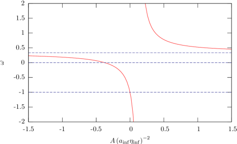
Figure 1: The equation of state that is required to maintain an exponential expansion depends on the coefficients of the corrections to GR, $A\left(a_{\rm inf}\eta_{\rm inf}\right)^{-2}$. Also plotted for comparison are the equations of state for a cosmological constant $\omega=-1$, pressureless matter $\omega=0$ and radiation $\omega=1/3$.

From (17) we see that exponential expansion is given by a fluid with a constant energy density just as for GR, however for a given energy density the Hubble rate, ${\cal H}$, will depend on the parameters of the theory ($\alpha$, $\beta$ and $\gamma$). In order to maintain the exponential expansion the equation of state parameter of the fluid, $\omega$ differs from the GR case ($\omega=-1$). Although it is a constant, it is important to note that this is only true for exactly exponential expansion with $K=0$, in general one would require a varying $\omega$. The equation of state that is required depends on the $\alpha$, $\beta$ and $\gamma$ and is plotted in Fig. (1), notice in particular for $8A=\left(a_{\rm inf}\eta_{\rm inf}\right)^{2}$ the equation of state that produces exponential expansion diverges, essentially meaning that it is not possible to have such expansion for these for a fluid with a finite pressure. However for $8A=\left(a_{\rm inf}\eta_{\rm inf}\right)^{2}$, (17) gives $\rho\left(a\right)=0$, thus it is not surprising that the pressure becomes ill defined. For this specific choice of parameters, the vacuum solution of the theory is an exponentially expanding cosmology. This divergence will appear again (for the $\alpha=0$ case) in Section III, when perturbations are considered.

From Fig. (1) we see that for $0<8A\left(a_{\rm inf}\eta_{\rm inf}\right)^{-2}<1$ a phantom fluid is required to produce the expansion i.e. $\omega<-1$, while for $8A\left(a_{\rm inf}\eta_{\rm inf}\right)^{-2}>1$ a fluid with $\omega>1/3$ is necessary. Finally for $A<0$ (i.e. $\alpha-3\beta<0$) exponential expansion can be achieved by fluids with $-1<\omega<1/3$. In particular, only $A=0$ (or equivalently $\alpha-3\beta=0$) will produce an exponential expansion in the presence of a slowly rolling scalar field (for which $\omega\approx-1$). The $A<0$ and $8A\left(a_{\rm inf}\eta_{\rm inf}\right)^{-2}>1$ cases could have the desired expansion driven by a scalar field if the kinetic and potential energies of the field were correctly matched, to give (18). However even if this does not result in excessive fine-tuning (over that required by standard inflation), it would likely be rather difficult to ensure that $\omega$ has the correct value over a long period of expansion.

Thus a period of exponential expansion, within general fourth derivative gravity theories is unlikely to be sourced by a simple scalar field, unless $A\ll 1$ (this is the case for example in Muller:1988db and Schmidt:1988hq ). However the presence of non-minimal couplings between the scalar field and the curvature terms can have a significant effect even in the $\alpha-3\beta=0$ case Nelson:2009wr ; Buck:2010sv ; Barvinsky:2009ii , so one cannot rule out the possibility. Indeed, the motivation for studying such corrections to GR requires that we consider $\alpha-3\beta$ be small (and hence $A$ to be small), in order to avoid super-luminal propagation (and other ghost effects, see Section I). With this in mind it is possible that standard slow roll inflation would result in almost exponential expansion i.e. that the deviations from the expected GR behaviour are small. Determining the observational consistency of such an approximation would require both a general solution to (12) in the presence of a scalar field and, eventually, details of the evolution of perturbations against this background.

If we want to have inflation driven by a scalar field in the standard way, the correction terms need to satisfy, $|A|\left(a_{\rm inf}\eta_{\rm inf}\right)^{-2}\ll 1$. Since this is a constant, it would imply that also at the end of the inflationary epoch $|A|\left(a_{\rm inf}\eta_{\rm inf}\right)^{-2}\ll 1$ and hence the radiation era would begin with this dimensionless ratio being small.

II.2 Radiation era

In standard GR an era dominated by a single fluid with $\omega=1/3$ (i.e. radiation) produces $a\left(\eta\right)=a_{\rm r}\eta/\eta_{\rm r}$, where $a_{\rm r}$ is the scale factor at $\eta_{\rm r}$, which is the conformal time at which the radiation era begins. Using this form of the scale factor in (12), we find that

$$\rho\left(a\right) = \frac{12\left(\alpha-3\beta\right)a_{\rm r}^{4}}{\eta_{\rm r}^{4}a^{8}}\left(4+2K\left(\frac{a\eta_{\rm r}}{a_{\rm r}}\right)^{2}-K^{2}\left(\frac{a\eta_{\rm r}}{a_{\rm r}}\right)^{4}\right)$$ (20)

$$+\frac{\gamma\kappa^{-2}a_{\rm r}^{2}}{\eta_{\rm r}^{2}a^{4}}\left(1+K\left(\frac{a\eta_{\rm r}}{a_{\rm r}}\right)^{2}\right)~{},$$

and

$$\rho\left(a\right)\left(1-3\omega\right) = -\frac{48\left(\alpha-3\beta\right)Ka_{\rm r}^{2}}{\eta_{\rm r}^{2}a^{6}}+\frac{12\gamma\kappa^{-2}K}{a^{2}}~{}.$$ (21)

Thus, if we restrict our attention to the $K=0$ case, we find that an expansion of $a\left(\eta\right)=a_{\rm r}\eta/\eta_{\rm r}$ is produced by a fluid with $\omega=1/3$ and

$$\rho\left(a\right)=\frac{6a_{\rm r}^{2}\gamma\kappa^{-2}}{\eta_{\rm r}^{2}a^{4}}\left(1+8\frac{Aa_{\rm r}^{2}}{\eta_{\rm r}^{2}a^{4}}\right)~{},$$ (22)

where $A$ is given in (19). Such a fluid has the equation of state of radiation, however the required energy density would be larger (for $\alpha-3\beta>0$) than that of radiation and would scale differently. Such corrections to the energy density would, however, rapidly become small as the universe expands and

$$8\frac{|A|a_{\rm r}^{2}}{\eta_{\rm r}^{2}a^{4}}\ll 1~{}.$$ (23)

As discussed in Section (II.1), if the radiation era is preceded by an epoch of inflation that is driven by a scalar field, then $8|A|\ll\left(a_{\rm r}\eta_{\rm r}\right)^{2}$ at the beginning of the radiation era. This would ensure that the expected expansion would approximately be achieved by standard radiation even early in the radiation era.

II.3 Matter era

Repeating the above procedure for matter era type expansion, i.e., $a\left(\eta\right)=a_{\rm m}\eta^{2}/\eta_{\rm m}^{2}$, where as in the previous two cases, we have defined the time the matter era began as $\eta_{\rm m}$ and the scale factor at this time to be $a_{\rm m}$. One then finds (again for the $K=0$ case) that the required energy density is,

$$\rho\left(a\right)=\frac{24\gamma\kappa^{-2}a_{\rm m}}{\eta_{\rm m}^{2}a^{3}}\left(1+34\frac{Aa_{\rm m}}{\eta_{\rm m}^{2}a^{3}}\right)~{}.$$ (24)

Thus, just as in the radiation case, the fluid would have to have a larger (for $\alpha-3\beta>0$) energy density than standard pressureless matter. These corrections would rapidly become very small as the universe expands, however, unlike the radiation era case where the usual equation of state was found, here we require,

$$\omega=\frac{2Aa_{\rm m}}{\eta_{\rm m}^{2}a^{3}}\left(1+34\frac{Aa_{\rm m}}{\eta_{\rm m}^{2}a^{3}}\right)^{-1}~{}.$$ (25)

Therefore an exactly pressureless fluid will not produce an expansion consistent with predictions of GR. However the pressure that is required to match the GR expectations is vanishingly small for

$$\frac{|A|a_{\rm m}}{\eta_{\rm m}^{2}a^{3}}\ll 1~{}.$$ (26)

Thus for large scales (or late times) the background cosmological evolution will be approximately the same as that expected from GR, provided

$$|A|\left(a_{\rm inf}\eta_{\rm inf}\right)^{-2}\ll 1~{}.$$ (27)

Considering for the moment only the radiation and matter eras, all that is required is that $|A|\left(a_{\rm r}\eta_{\rm r}\right)^{-2}$ be sufficiently small, so as to allow (22) to be approximately correct for standard radiation. As the universe expands the evolution will then quickly approach the standard cosmology of GR. For $|A|\left(a_{\rm inf}\eta_{\inf}\right)^{-2}\ll 1$ this is satisfied and hence the standard background dynamics can be (approximately) reproduced from a slowly rolling scalar field, with the corrections to the GR expectations remaining small throughout the history of the universe. This agrees with the conclusions of Macrae:1981ic .

We have considered only the flat ($K=0$) case, the presence of a non-zero curvature would introduce additional corrections to the standard GR evolution equations. However it is clear from (II.1), (20) and (21) (and similarly for the analogous equations for the matter era) that the consequences of $K\neq 0$ rapidly become small in a large scale, expanding universe. This is to be expected since the energy density associated with the spatial curvature of an expanding universe decreases with time, hence its consequences will diminish.

III Tensor mode perturbations

In the previous sections we derived the evolution of the background cosmology for a general $4^{\rm th}$ order correction to GR. Given the prevalence of ghost modes in such theories, it is important to examine the evolution of perturbations on these background cosmologies. Here we derive the equations governing the dynamics of cosmological gravitational waves. See Bogdanos:2009tn for an alternative derivation in a more general setting and Noh:1996da for an derivation similar to the one presented here. Also Hwang:2001pu for the generation and evolution of tensor modes during inflation for a specific $f(R)$ model, which includes a detailed analysis of the properties of the resulting spectrum.

A general perturbation to the metric, (8), can be decomposed into scalar, vector and tensor components (see for example durrer_book ) and here we will be concerned only with the tensor modes, which are transverse and traceless and given by the perturbed metric,

$$\delta g_{00}=\delta g_{0i}=0~{},~{}~{}~{}~{}\delta g_{ij}=2a^{2}\left(\eta\right)E_{ij}~{},$$ (28)

where the perturbation $E_{ij}$ is transverse ($D^{i}E_{ij}=0$) and traceless ($\bar{g}^{ij}E_{ij}=0$), the non-transverse and non-traceless parts giving contributions to the vector and scalar perturbations respectively. Using this perturbed metric one finds the perturbations to the components of the Riemann tensor,

$$\delta R^{0}_{~{}i0j}=-\left(E^{\prime\prime}_{ij}+{\cal H}E^{\prime}_{ij}+2{\cal H}^{\prime}E_{ij}\right)~{},~{}~{}~{}~{}\delta R^{0}_{~{}ijk}=E^{\prime}_{ij|k}-E^{\prime}_{ik|j}~{},$$

$$\delta R^{i}_{~{}00j}=\left(E^{\prime\prime}\right)^{i}_{~{}j}+{\cal H}\left(E^{\prime}\right)^{i}_{~{}j}~{},~{}~{}~{}~{}\delta R^{i}_{~{}0jk}=-\left(E^{\prime}\right)^{i}_{~{}k|j}+\left(E^{\prime}\right)^{i}_{~{}j|k}~{}$$

$$\delta R^{i}_{~{}j0k}=-\left(E^{\prime}\right)^{~{}~{}|i}_{jk}-\left(E^{\prime}\right)^{i}_{~{}k|j}~{},$$

$$\delta R^{i}_{~{}jmn}=-2{\cal H}^{2}\left(\delta^{i}_{m}E_{jn}-\delta^{i}_{n}E_{jm}\right)$$

$$~{}~{}~{}~{}~{}~{}~{}~{}~{}~{}~{}-\left(E^{i}_{~{}j|nm}-E^{i}_{~{}j|mn}+E^{i}_{~{}n|jm}-E^{i}_{~{}m|jn}+E^{~{}~{}~{}|i~{}}_{jm~{}|n}-E^{~{}~{}|i~{}}_{jn~{}|m}\right)$$

$$~{}~{}~{}~{}~{}~{}~{}~{}~{}~{}~{}-{\cal H}\left(\delta^{i}_{m}\left(E^{\prime}\right)_{jn}-\delta^{i}_{n}\left(E^{\prime}\right)_{jm}-\left(E^{\prime}\right)^{i}_{~{}n}\gamma_{jm}+\left(E^{\prime}\right)^{i}_{~{}m}\gamma_{jn}\right)~{},$$ (29)

where $E_{ij|k}=D_{k}E_{ij}$ is the spatial covariant derivative of $E_{ij}$. Similarly one can calculate the perturbations to the remaining tensor components given in (II), the only non-zero expression being,

$$\delta R^{i}_{~{}j}=\frac{1}{a^{2}}\left(-\left(E^{\prime\prime}\right)^{i}_{~{}j}-2{\cal H}\left(E^{\prime}\right)^{i}_{~{}j}+\left(\Delta-K\right)E^{i}_{~{}j}\right)~{},$$ (30)

where $\Delta=D^{i}D_{i}$ is the spatial Laplacian. Note also that, because $E_{ij}$ is traceless, we have $\delta g^{i}_{~{}i}=0$, and hence $\delta G^{i}_{~{}j}=\delta R^{i}_{~{}j}$.

With this one can calculate the perturbations to (5) to find,

$$\delta H^{\mu}_{~{}\nu}=\left(\alpha-2\beta\right)\delta\left(R^{;\mu}_{~{}~{};\nu}\right)-\alpha\delta\left(R^{\mu~{};\rho}_{~{}\nu~{}~{};\rho}\right)-\left(\frac{\alpha}{2}-2\beta\right)\bar{g}^{\mu}_{~{}\nu}\delta\left(R^{;\rho}_{~{};\rho}\right)+2\alpha\left(\delta R\right)^{\rho\lambda}\bar{R}^{\mu}_{~{}\rho\nu\lambda}$$

$$+2\alpha\bar{R}^{\rho\lambda}\left(\delta R\right)^{\mu}_{~{}\rho\nu\lambda}+\left(\gamma\kappa^{-2}-2\beta\bar{R}\right)\left(\delta R\right)^{\mu}_{~{}\nu}=\frac{-1}{2}\delta T^{\mu}_{~{}\nu}~{}.$$ (31)

Of the various terms appearing in (III) those not involving covariant derivatives are the easiest to calculate. Using (III) and (30), one immediately finds,

$$\left(\delta R\right)^{\rho\lambda}\bar{R}^{i}_{~{}\rho j\lambda}=-\frac{\left({\cal H}^{2}+K\right)}{a^{4}}\left(\left(E^{\prime\prime}\right)^{i}_{~{}j}+2{\cal H}\left(E^{\prime}\right)^{i}_{~{}j}-\left(2{\cal H}^{\prime}+4{\cal H}^{2}+\Delta+2K\right)E^{i}_{~{}j}\right)~{},$$ (32)

and

$$\bar{R}^{\rho\lambda}\left(\delta R\right)^{i}_{~{}\rho j\lambda} = \frac{1}{a^{4}}\Bigl{(}-3{\cal H}^{\prime}\left(E^{\prime\prime}\right)^{i}_{~{}j}-2{\cal H}^{\prime}{\cal H}\left(E^{\prime}\right)^{i}_{~{}j}$$ (33)

$$+6\left({\cal H}^{2}+K\right){\cal H}\left(E^{\prime}\right)^{i}_{~{}j}-\left({\cal H}^{\prime}+2\left({\cal H}^{2}+K\right)\right)\left(2{\cal H}^{2}+\Delta\right)E^{i}_{~{}j}\Bigr{)}~{},$$

while since only tensor perturbations are being considered the remaining components vanish.

Calculating the terms in (III) that involve covariant derivatives is rather more involved however it is easily achieved by expanding out the covariant derivatives in terms of the metric and its derivatives. Here we quote the results, with the (tedious) calculation given in Appendix B.

$$\delta\left(R^{;\rho}_{~{}~{};\rho}\right) = \delta\left(R^{;0}_{~{}~{};0}\right)=\delta\left(R^{;0}_{~{}~{};i}\right)=0~{},$$

$$\delta\left(R^{;i}_{~{}~{};j}\right) = \frac{-1}{a^{2}}\bar{R}^{\prime}\left(E^{\prime}\right)^{i}_{~{}j}~{},$$

$$\delta\left(R^{0~{};\rho}_{~{}0~{};\rho}\right) = \delta\left(R^{0~{};\rho}_{~{}i~{};\rho}\right)=0~{},$$

$$\delta\left(R^{i~{};\rho}_{~{}j~{};\rho}\right) = \frac{8}{a^{4}}{\cal H}\left({\cal H}^{\prime}-{\cal H}^{2}-K\right)\left(E^{\prime}\right)^{i}_{~{}j}$$ (34)

$$+\frac{1}{a^{2}}{\cal D}\left(\frac{1}{a^{2}}\left(-\left(E^{\prime\prime}\right)^{i}_{~{}j}-2{\cal H}\left(E^{\prime}\right)^{i}_{~{}j}+\left(\Delta-K\right)E^{i}_{~{}j}\right)\right)~{},$$

where in the last equation, the differential operator ${\cal D}$ is defined as

$${\cal D}\equiv\left(-\frac{\partial^{2}}{\partial\eta^{2}}-2{\cal H}\partial_{\eta}+2{\cal H}^{2}+\Delta\right)~{}.$$ (35)

Using the expressions given in (III) one readily finds that the evolution equation for tensor mode perturbations, (III), becomes

$$\delta H^{i}_{~{}j}=\frac{1}{a^{4}}\Bigl{[}-\alpha\left(E^{\prime\prime\prime\prime}\right)^{i}_{~{}j}+\left(\alpha_{1}+2\alpha\Delta\right)\left(E^{\prime\prime}\right)^{i}_{~{}j}+\alpha_{2}\left(E^{\prime}\right)^{i}_{~{}j}$$

$$+\left[\left(\Delta-K\right)\left(\alpha_{3}-\alpha\Delta\right)+\alpha_{4}-2\alpha\left({\cal H}^{\prime}+2{\cal H}^{2}+2K\right)\Delta\right]E^{i}_{~{}j}\Bigr{]}~{},$$

where we have defined the $\eta$ dependent functions,

$$\alpha_{1} \equiv -4{\cal H}^{\prime}\left(2\alpha+3\beta\right)+4{\cal H}^{2}\left(\alpha-3\beta\right)-3K\left(\alpha+4\beta\right)-\frac{\gamma a^{2}}{\kappa^{2}}~{},$$

$$\alpha_{2} \equiv 4{\cal H}^{\prime\prime}\left(\alpha-3\beta\right)+8\alpha{\cal H}^{3}+6\alpha{\cal H}K-4{\cal H}{\cal H}^{\prime}\left(\alpha+6\beta\right)-\frac{2\gamma a^{2}{\cal H}}{\kappa^{2}}~{},$$

$$\alpha_{3} \equiv -2{\cal H}^{\prime}\left(\alpha-6\beta\right)+12\beta{\cal H}^{2}+2K\left(\alpha+6\beta\right)+\frac{\gamma a^{2}}{\kappa^{2}}~{},$$

$$\alpha_{4} \equiv 6\alpha{\cal H}^{2}K+4\alpha K{\cal H}^{\prime}+6\alpha K^{2}~{}.$$ (37)

Notice in particular that the degeneracy present in the background equations between $\alpha$ and $\beta$ is now broken and the particular combination $\alpha-3\beta$ play no special role in the perturbation equations. This agrees with the results of Nelson:2008uy ; Nelson:2010rt , which showed that deviations from standard cosmology for NCG inspired corrections to GR (for which $\alpha=3\beta$), are important for perturbations in general and gravitational waves in particular. Indeed, by restricting our attention to flat Minkowski space-time, i.e., ${\cal H}=0$ and $K=0$, and taking $\alpha=3\beta$, (III) reduces to the equation for gravitational radiation derived in Nelson:2010rt .

IV Tensor Perturbations Against Different Cosmological Backgrounds

The general evolution equation given in (III) can be simplified by considering specific forms of background evolution. For example, consider $a\left(\eta\right)=a_{\rm i}\eta_{\rm i}^{-\nu}\eta^{\nu}$ for some constants $\nu$, $a_{\rm i}$ and $\eta_{\rm i}$. Such power law behaviour is typical in cosmologies dominated by a single matter fluid in GR e.g. $\nu=2$ corresponds to the matter dominated era, while $\nu=1$ gives the radiation dominated era, with $a_{\rm i}$ and $\eta_{\rm i}$ being the scale factor and conformal time at the beginning of these eras respectively (see Section II). One can easily extend this to include several matter fields and hence allow for (for example) the transition from the radiation to matter dominated eras, however for simplicity we focus on single fluid systems. Here we have kept $\alpha$ and $\beta$ general, however it must be remembered that if (for example) $a\left(\eta\right)\propto\eta$ is to represent the expansion during a radiation dominated era, then we must satisfy (23).

Decomposing all spatial functions into eigenfunctions, $Q_{\bf k}$ of the spatial Laplacian i.e. $\Delta Q_{\bf k}=-|{\bf k}|^{2}Q_{\bf k}$  so that in particular $\Delta E^{i}_{~{}j}=-|{\bf k}|^{2}E^{i}_{~{}j}$, one finds,

$$\delta H^{i}_{~{}j}\Big{|}_{\rm powerlaw}=\left(\frac{|{\bf k}|}{a_{\rm i}}\right)^{4}\left(\frac{x_{\rm i}}{x}\right)^{4\nu}\Biggl{[}-\alpha\frac{{\rm d}^{4}E^{i}_{~{}j}}{{\rm d}x^{4}}+\left(-\beta_{1}+\frac{\beta_{2}}{x^{2}}-{\cal K}\left(\frac{x}{x_{\rm i}}\right)^{2\nu}\right)\frac{{\rm d}^{2}E^{i}_{~{}j}}{{\rm d}x^{2}}$$

$$+\left(6\alpha\nu\frac{K}{|{\bf k}|^{2}}+\frac{\beta_{3}}{x^{2}}-2\nu{\cal K}\left(\frac{x}{x_{\rm i}}\right)^{2\nu}\right)\frac{1}{x}\frac{{\rm d}E^{i}_{~{}j}}{{\rm d}x}$$

$$+\left(\beta_{4}+\frac{\beta_{5}}{x^{2}}+x^{2}\beta_{6}-{\cal K}\left(\frac{x}{x_{\rm i}}\right)^{2}\left(\frac{K}{|{\bf k}|^{2}}+1\right)\right)E^{i}_{~{}j}\Biggr{]}~{},$$ (38)

where

$$\beta_{1} = 2\alpha+3\left(\alpha+4\beta\right)\frac{K}{|{\bf k}|^{2}}~{},$$

$$\beta_{2} = 4\nu\left(2\alpha+3\beta+\nu\left(\alpha-3\beta\right)\right)~{},$$

$$\beta_{3} = 8\nu^{3}\alpha+4\nu^{2}\left(\alpha+6\beta\right)+8\nu\left(\alpha-3\beta\right)~{},$$

$$\beta_{4} = 4\left(\alpha-3\beta\right)\left(\frac{K}{|{\bf k}|^{2}}\right)^{2}+4\alpha\left(\frac{K}{|{\bf k}|^{2}}\right)-\alpha-2\nu\left(\alpha-6\beta\right)-12\nu^{2}\beta~{},$$

$$\beta_{5} = 6\nu\left(\nu\left(\alpha-2\beta\right)-\alpha+2\beta\right)\left(\frac{K}{|{\bf k}|^{2}}\right)+2\alpha\nu\left(2\nu-1\right)~{},$$

$$\beta_{6} = -3\left(\alpha-4\beta\right)\left(\frac{K}{|{\bf k}|^{2}}\right)~{},$$ (39)

and we have changed variables to $x=\eta|{\bf k}|$ and defined the (dimensionless) variables $x_{\rm i}\equiv|{\bf k}|\eta_{\rm i}$ and

$${\cal K}\equiv\frac{\gamma}{\kappa^{2}}\left(\frac{a_{\rm i}}{|{\bf k}|}\right)^{2}~{}.$$ (40)

Note that if ${\cal K}\gg\alpha,\beta$, then (IV) approximates the usual GR evolution equation for tensor modes (e.g. durrer_book ), as it should. In particular then the evolution of extremely large scale modes (i.e. modes for which $|{\bf k}|\ll 1$) is precisely that of GR. Of course, here one has to be careful, since the GR limit of Eq. (IV) reduces the order of the perturbation equation and hence can introduce strong instabilities. One can, however check that if the solution matches the GR solution initially, then it will continue to do so throughout the evolution. Furthermore, one can estimate the magnitude of the effect of small deviations to the GR solution, by evaluating the higher derivative terms appearing in Eq. (IV) for the (approximate) GR solutions. Doing this one finds that the corrections seem to remain small during the evolution of the modes, however such evidence does not remove the possibility of their being a growing mode to the corrections to the GR solutions, even in the ${\cal K}\gg\alpha,\beta$ limit. However, if such an instability were present, it would likely involve a significant growth in the amplitude of $\delta H^{i}_{~{}j}$ and hence would result in even stronger constraints than those presented below.

Of particular interest is the evolution of tensor modes in a flat ($K=0$) universe, during the radiation era. Recall for such a radiation dominated universe we have $\nu\approx 1$ (see the discussion below (22)). One immediately sees that for $\nu=1$ the coefficients given in (IV) are independent of $\beta$. Hence the propagation of tensor modes during the radiation era are unaffected by the presence of $R^{2}$ corrections, for a flat universe, regardless of the strength of the coupling $\beta$. Assuming that the universe is exactly flat, the evolution during the radiation era ($\nu=1$) for a general $\alpha$ is given by,

$$\delta H^{i}_{~{}j}=\alpha\left(\frac{|{\bf k}|}{a_{\rm i}}\right)^{4}\left(\frac{x_{\rm i}}{x}\right)^{4}\Biggl{[}-\frac{{\rm d}^{4}E^{i}_{~{}j}}{{\rm d}x^{4}}+\left(\frac{12}{x^{2}}-2-\frac{\cal K}{\alpha}\left(\frac{x}{x_{\rm i}}\right)^{2}\right)\frac{{\rm d}^{2}E^{i}_{~{}j}}{{\rm d}x^{2}}$$

$$\left(\frac{20}{x^{2}}-\frac{2{\cal K}}{\alpha}\left(\frac{x}{x_{\rm i}}\right)^{2}\right)\frac{1}{x}\frac{{\rm d}E^{i}_{~{}j}}{{\rm d}x}+\left(\frac{2}{x^{2}}-3-\frac{{\cal K}}{\alpha}\left(\frac{x}{x_{\rm i}}\right)^{2}\right)E^{i}_{~{}j}\Biggr{]}~{}.$$ (41)

Hence, the evolution will be well approximated by that of GR when

$$\frac{\cal K}{\alpha}\left(\frac{x}{x_{\rm i}}\right)^{2}\gg 1~{},$$ (42)

which is true at late times, i.e., large $x$, (recall however the comments below Eq. (40)).

If we consider the evolution of perturbations to a flat inflationary era i.e. with $K=0$ and $\nu=-1$, and consider only $R^{2}$ corrections i.e. $\alpha=0$, we find that (IV) factorises into

$$\delta H^{i}_{~{}j}\Big{|}_{\nu=-1,~{}\alpha=0,~{}K=0}=$$

$$-\left(\frac{|{\bf k}|}{a}\right)^{4}\left(\frac{x}{x_{\rm i}}\right)^{2}\left(\frac{24\beta}{x^{2}_{\rm i}}+{\cal K}\right)\left(\frac{{\rm d}^{2}E^{i}_{~{}j}}{{\rm d}x^{2}}-\frac{2}{x}\frac{{\rm d}E^{i}_{~{}j}}{{\rm d}x}+E^{i}_{~{}j}\left(x\right)\right)~{}.$$ (43)

The differential equation in parenthesis is precisely that of General Relativity, thus, in the absence of a source, the evolution of tensor mode perturbations during inflation (with $K=0$), is unaffected by the presence of $R^{2}$ corrections (provided there are no $R^{\mu\nu}R_{\mu\nu}$ corrections). Note however that although the evolution of these modes is independent of such corrections, their generation will not be. As can be seen from (IV) the effect of the $R^{2}$ correction is to introduce an effective, Newtonian constant

$$a^{2}_{\rm i}\frac{\gamma}{\kappa^{2}}\rightarrow a^{2}_{\rm i}\frac{\gamma}{\kappa^{2}}+24\frac{\beta}{\eta_{\rm i}^{2}}~{}.$$ (44)

In particular there is a critical value at $24\beta\kappa^{2}=-\gamma\left(a_{\rm i}\eta_{\rm i}\right)^{2}$ at which the evolution becomes ill defined. This is precisely the same divergence found for the background evolution in Section (II.1). The vanishing of the prefactor in (IV) makes the evolution arbitrarily sensitive to any deviations for this equation of motion (i.e. the evolution is unstable), which is to be expected for perturbations about such a pathological background cosmology.

We mention in passing that for the specific ratio $\alpha=24\beta$ and $K=0$, (IV) can be exactly solved. The resulting expression, involving hypergeometric functions, is not, however, particularly illuminating.

V Constraining modifications to GR

As mentioned in Section I, local tests of GR, particularly from the perihelion precession of Mercury Stelle:1977ry and the production of gravitational waves from binaries Nelson:2010ru , provide only very weak constraints, typically of the order of $\left(\alpha-3\beta\right)<10^{70}$. Cosmology has the advantage over such test, both because it is possible to reach higher curvature regimes in the early universe and also because we naturally have very long evolution times, during which even small deviations from GR can become significant. As we found in Section II, in order for a slowly rolling scalar field to have sustained the exponential expansion of inflation, in the usual way, we require

$$\left(\frac{|\alpha-3\beta|}{\gamma\kappa^{-2}}\right)\left(\frac{1}{a_{\rm inf}\eta_{\inf}}\right)^{2}\ll 1~{},$$ (45)

where recall $a_{\rm inf}$ and $\eta_{\rm inf}$ are the scale factor and conformal time at the beginning of inflation. Note that $\eta$ is conformal time, so $a_{\rm inf}\eta_{\rm inf}=t_{\inf}$, where $t_{\rm inf}$ is the cosmic time at the beginning of inflation. Taking inflation to have occurred $t\approx t_{0}\times 10^{-40}\approx 10^{-22}{\rm sec}$ kolb_turner , where $t_{0}$ is the current cosmic time (taken to be approximately $10^{18}{\rm sec}$), we see that (45) becomes,

$$\left(\frac{|\alpha-3\beta|}{\gamma\kappa^{-2}}\right)\ll 10^{-80}t_{0}^{2}~{},$$ (46)

or, taking $\gamma\kappa^{-2}=\left(16\pi G\right)^{-1}$ and using the experimental value of Newton’s constant ($G\approx 2.88\times 10^{-87}{\rm sec}^{2}$ in these units),

$$|\alpha-3\beta|\ll 6.7\times 10^{40}~{}.$$ (47)

While this constraint may still seem rather weak it is an improvement by some thirty orders of magnitude over the previous best astrophysical constraints (and is twenty orders of magnitude better than laboratory tests).

One may be concerned that this constraint is produced by assuming that inflation is produced by a slowly rolling scalar field. Maybe there is some other mechanism for producing the exponential expansion required to solve the horizon, curvature and monopole problems of the standard big-bang theory? Indeed, there are examples of higher derivative theories driving inflation directly Starobinsky:2001xq ; Nelson:2009wr . Or perhaps there is an alternative to inflation that does not require such exponential expansion? Certainly, since we have yet to derive the consequences of this general $4^{\rm th}$ order theory on the growth (or otherwise) of scalar perturbations, it is premature to suggest that such an expansion phase would produce the scale invariant perturbation spectrum required by the CMB.

To avoid these difficulties let us take the more conservative point of view and assume that the dynamics of the universe closely match those expected from GR only after some time, $t_{c}$, in the radiation era. Certainly the success of the CMB tells us that GR is a good approximation significantly before decoupling (i.e. before the last scattering surface). From (23) we then have

$$\left(\frac{|\alpha-3\beta|}{\gamma\kappa^{-2}}\right)\frac{1}{t_{\rm r}^{2}}\left(\frac{a_{\rm r}}{a_{\rm c}}\right)^{2}\ll 1~{},$$ (48)

where $t_{\rm r}$ is the cosmic time at the beginning of the radiation era and $a_{\rm r}$ and $a_{\rm c}$ are the scale factors at cosmic times $t_{\rm r}$ and $t_{\rm c}$ respectively. Being extremely conservative, let us assume that the universe was radiation dominated at energy scales below electro-weak unification ($t_{\rm EW}\sim 10^{-12}{\rm sec}$) $t_{\rm r}\sim 10^{-28}t_{0}$. Further let us assume that the universe is well approximated by that of GR at the scales on which Big Bang Nucleosynthesis takes place, $t_{\rm c}\approx 10^{-18}t_{0}$ kolb_turner . This assumptions gives

$$\frac{|\alpha-3\beta|}{\gamma\kappa^{-2}}\ll 10^{-50}t_{0}^{2}~{},$$ (49)

or, putting in the current age of the universe and Newton’s constant, $|\alpha-3\beta|\ll 10^{70}$. Thus even with these extremely conservative estimates, the constraint is the same as that from gravitational waves and solar system tests.

While the estimates above can provide a significant improvement on existing constraints, in the background equations there is a degeneracy in the parameters, in that we can restrict only the combination $\alpha-3\beta$. In order to place independent constraints on each parameter, we need to consider perturbations around the background cosmology. Using the results of Section IV we see that, during the radiation era, the evolution of the cosmological gravitational waves will deviate significantly from the predictions of GR unless,

$$\frac{\cal K}{\alpha}\left(\frac{x}{x_{\rm i}}\right)^{2}\gg 1~{}.$$ (50)

As a specific example, consider a mode that crosses the Horizon at matter-radiation equality, which occurs at $t_{\rm eq}\sim 10^{12}{\rm sec}$, and again conservatively consider the beginning of the radiation dominated era to be at the electro-weak scale. One then finds that (50) reduces to,

$$\alpha\ll 6.7\times 10^{70}~{},$$ (51)

again comparable to the current best constraints on such parameters. As is clear from (50), this constraint can be improved in two ways; by decreasing $x/x_{\rm i}$ i.e. considering the modes close to the beginning of the radiation era or by decreasing ${\cal K}$. Recall from (40) that ${\cal K}\propto|{\bf k}|^{-2}$, thus the constraint can be improved by considering smaller wavelength gravitational waves (i.e. larger $|{\bf k}|$). The fact that these deviations from GR become more significant at small scales might have been expected because of the fact that these modes are ghosts Clunan:2009er .

Taking the point of view that this theory is only an effective theory, good down to some scale, after which some more complete theory will dictate the evolution of these modes, we require only that the deviation for GR be not significant (i.e. that the ghosts are not apparent) on observational scales. The use of the word observational here deserves some comment, since we have yet to observe cosmological gravitational waves at any scale! However the deviations from GR will typically make the tensor perturbations grow (as they represent an instability). If such growth had occurred and been significant, we would have observed their contribution to the galaxy power spectrum and the CMB. A quantitative constraint would require an in-depth analysis of the exact evolution given in (IV) and an understanding of the rate of the growth of the modes that can be expected. However in order to get an estimate on the order of magnitude of the constraint, we will simply require that the deviations from GR be small at the smallest observable scales at which such cosmological tensor modes could have been observed i.e. for the first modes that entered the horizon that have been observed in the galaxy power spectra.

Data from Lyman alpha forests Tegmark:2001jh ; Tegmark:2002cy provide us with a detailed power spectrum of (scalar) density perturbations that matches the expectations of GR down to scales $|{\bf k}|\sim\left(10^{2}\--10^{3}\right)|{\bf k}|_{\rm equality}$, where $|{\bf k}|_{\rm equality}$ is the scale at matter radiation equality (which produces the characteristic peak in the power spectrum). Thus at such scales the constraint is improved by a factor of $10^{4}\--10^{6}$ over (51). This improvement would be further increased by considering smaller scales or, of course, by direct measurement of the cosmological gravitational wave background.

VI Conclusions

We have shown that it is possible to approximately reproduce the key epochs of standard cosmology within a generally modified $4^{\rm th}$ order gravity theory. More precisely we demonstrated that only a correction to Einstein-Hilbert gravity of the form $C^{\mu\nu\rho\gamma}C_{\mu\nu\rho\gamma}$ introduces no deviation from standard background cosmology, while any other correction can approximate the standard background evolution, provided it is initially ‘close’ to such a correction (see Section II for a more precise statement). Furthermore by requiring that the deviations from GR be small at certain key eras (such as during inflation and Big Bang Nucleosynthesis) we can quantify how ‘close’ general corrections need to be in order to be consistent. Even taking the conservative point of view that radiation domination began only after the electroweak scale, such constraints are comparable to the best current restrictions on the theory. Further requiring that inflation be sourced by a fluid with $\omega\approx-1$ allowed us to improve this constraint by thirty orders of magnitude! The appearance of such large constraints is not uncommon within cosmology. Consider for example the spatial curvature within non-inflationary cosmology. If the energy density associated with such curvature vanishes to one part in $10$ today, it would have to vanish to one part in $10^{60}$ close to the Grand Unification scale. Indeed this was one of the original motivations for inflation. Similarly requiring that the higher order curvature corrections be small today is a much weaker constraint than requiring they be small in the past. The earlier we can examine the consequences of such corrections (such as during the radiation era or inflation) the more the constraints can be improved.

At the background level we are able only to constrain the parameter $\alpha-3\beta$ ($\alpha=3\beta$ corresponds to the $C^{\mu\nu\rho\gamma}C_{\mu\nu\rho\gamma}$ correction of Non-commutative Geometry) and not the individual coefficients. In order to break this degeneracy we consider the evolution of perturbations against the homogeneous and isotropic background. For comparison with observations, one would like to examine the scalar perturbations of such a theory, which can be directly related to the galaxy power spectrum, weak lensing surveys, and the CMB. However the equations governing the evolution of scalar perturbation are extremely involved in a general $4^{\rm th}$ order gravity theory, making their use difficult. Instead we focused on the evolution of tensor modes (cosmological gravitational waves), which are technically simpler to calculate. While they have yet to be observed, they have the additional advantage of not coupling directly to matter (in the absence of anisotropic stress). Thus they are independent of any corrections to the matter action and are direct probes of the underlying geometry of the problem.

Without direct observational evidence of such tensor mode perturbations, we considered the types of gravitational theories for which the evolution is approximately that of GR. The fact that such theories will typically lead to instabilities of perturbations, suggests that deviations from GR will include a strong growth of the amplitude of the perturbations. Had this occurred the perturbations would have been observed and hence our constraint is equivalent to ensuring that such instabilities occur at scales that are not (yet) observable.

We showed that the presence of $R^{2}$ corrections to GR does not affect the evolution of tensor mode perturbations in a flat radiation dominated universe, while if only $R^{2}$ corrections are present, there is also no effect on the evolution, during the inflation era (although one can expect an affect on their production). Requiring that corrections be small for a specific mode and a particular scale (within the radiation era) hence constrains the coefficient of $R^{\mu\nu}R_{\mu\nu}$ corrections and breaks the degeneracy present in the background equations.

By considering modes that have contributed to the measured (scalar) power spectrum we can estimate the constraint on $R^{\mu\nu}R_{\mu\nu}$ corrections, finding it to be improved by factor of $10^{4}\--10^{6}$ over current best restrictions. Thus, if inflation is to have occurred in the usual manner, we require

$$\alpha-3\beta\ll{\cal O}\left(10^{40}\right)~{},~{}~{}~{}~{}\alpha\ll{\cal O}\left(10^{65}\right)~{},$$ (52)

which is a remarkable improvement on current constraints which give $\alpha,~{}\beta\ll{\cal O}\left(10^{70}\right)$.

Finally it is important to note that the presence of ghost in theories with such $4^{\rm th}$ order corrections is well known Stelle:1977ry and clearly indicates that the theory cannot be a fundamental theory (and certainly cannot be quantised in any standard way). Thus one should consider such corrections as an effective theory, which is valid in some range of scales and replaced by some more complete theory outside that range. For example, such corrections occur in the asymptotic expansion of certain Non-commutative Geometry theories Chamseddine:2010ud , (in that case $\alpha=3\beta$) and beyond a specific scale the space-time is no longer even approximately commutative. Here we have shown that the presence of ghosts is not felt at the level of background cosmology, however it is crucial for the evolution of perturbations and the constraints produced here essentially ensure that the presence of ghosts would not effect observable scales. One expects that higher (i.e. $6^{\rm th}$ and higher Gottlober:1989ww ; Hwang:1991 ) order corrections to (4) would become significant some scale. The presence of ghosts indicate the scale at which these higher order terms would need to become significant and essentially mark the scale at which the ($4^{\rm th}$ order) effective theory begins to break down. Thus the constraints produced here can be viewed as determining the scale at which (4) is a valid effective theory. It is important to note however, that here we have assumed a perturbative expansion and it is possible that non-perturbative effects might be significant.

Appendix A

In this appendix we derive the time-time component and trace of the tensor $H^{\mu}_{~{}\nu}$ given in (5), for the background FRW metric, (8). First note that the non-zero Christoffel symbols associated with this metric are,

$$\bar{\Gamma}^{0}_{00}={\cal H}~{},~{}~{}~{}~{}\bar{\Gamma}^{i}_{j0}={\cal H}\delta^{i}_{~{}j}~{},~{}~{}~{}~{}\bar{\Gamma}^{0}_{ij}={\cal H}\gamma_{ij}~{},~{}~{}~{}~{}\bar{\Gamma}^{k}_{ij}=~{}^{(3)}\bar{\Gamma}^{k}_{ik}~{},$$ (53)

where ${}^{(3)}\bar{\Gamma}^{k}_{ij}$ is the three dimensional Christoffel symbol calculated from the spatial metric $\gamma_{ij}$. In order to evaluate the components of (5) we need,

$$\bar{R}^{\mu~{};\rho}_{~{}\nu~{};\rho} = \frac{-1}{a^{2}}\left(\bar{f}^{\mu}_{~{}\nu 0,0}+\bar{\Gamma}^{\mu}_{0\alpha}\bar{f}^{\alpha}_{~{}\nu 0}-\bar{\Gamma}^{\alpha}_{\nu 0}\bar{f}^{\mu}_{~{}\alpha 0}-\bar{\Gamma}^{\alpha}_{~{}00}\bar{f}^{\mu}_{~{}\nu\alpha}\right)$$ (54)

$$+\frac{\gamma^{ij}}{a^{2}}\left(\bar{\Gamma}^{\mu}_{i\alpha}f^{\alpha}_{~{}\nu j}-\bar{\Gamma}^{\alpha}_{\nu i}\bar{f}^{\mu}_{~{}\alpha j}-\bar{\Gamma}^{\alpha}_{ji}\bar{f}^{\mu}_{~{}\nu\alpha}\right)~{},$$

where we have defined $\bar{f}^{\mu}_{~{}\nu\alpha}\equiv\bar{R}^{\mu}_{~{}\nu;\alpha}$, which has non-zero components,

$$\bar{f}^{0}_{~{}00} = \frac{3}{a^{2}}\left(2{\cal H}{\cal H}^{\prime}-{\cal H}^{\prime\prime}\right)~{},$$

$$\bar{f}^{0}_{~{}ij} = \frac{2{\cal H}}{a^{2}}\gamma_{ij}\left({\cal H}^{\prime}-{\cal H}^{2}-K\right)~{},$$

$$\bar{f}^{i}_{~{}0j} = \frac{-2{\cal H}}{a^{2}}\delta^{i}_{~{}j}\left({\cal H}^{\prime}-{\cal H}^{2}-K\right)~{},$$

$$\bar{f}^{i}_{~{}j0} = -\delta^{i}_{~{}j}\left(\frac{1}{a^{2}}\left({\cal H}^{\prime}+2\left({\cal H}^{2}+K\right)\right)\right)^{\prime}~{}.$$ (55)

Thus we find,

$$\bar{R}^{0~{};\rho}_{~{}0~{};\rho} = \frac{-3}{a^{4}}\left(2\left({\cal H}^{\prime}\right)^{2}+2{\cal H}{\cal H}^{\prime\prime}-{\cal H}^{\prime\prime\prime}+4{\cal H}^{2}{\cal H}^{\prime}-4{\cal H}^{4}-4{\cal H}^{2}K\right)~{},$$

$$\bar{R}^{\gamma~{};\rho}_{~{}\gamma~{};\rho} = \frac{6}{a^{4}}\left({\cal H}^{\prime\prime\prime}-2{\cal H}^{\prime}\left(K+3{\cal H}^{2}\right)\right)~{}.$$ (56)

In addition we need $\bar{R}^{;0}_{~{};0}$ and $\bar{R}^{;\rho}_{~{};\rho}$ which are,

$$\bar{R}^{;0}_{~{};0} = \frac{6}{a^{4}}\left(-6{\cal H}^{2}{\cal H}^{\prime}-3{\cal H}{\cal H}^{\prime\prime}+6{\cal H}^{2}\left({\cal H}^{2}+K\right)-2{\cal H}^{\prime}K+{\cal H}^{\prime\prime\prime}\right)~{},$$

$$\bar{R}^{;\rho}_{~{};\rho} = \frac{6}{a^{4}}\left({\cal H}^{\prime\prime\prime}-6{\cal H}^{2}{\cal H}^{\prime}-2{\cal H}K\right)~{}.$$ (57)

Using the expressions given in (II) one directly finds the remaining terms in $H^{0}_{~{}0}$ and $H^{\rho}_{~{}\rho}$, eventually giving,

$$\bar{H}^{0}_{~{}0} = \frac{6\left(\alpha-3\beta\right)}{a^{4}}\left[-2{\cal H}\left({\cal H}^{\prime\prime}+2{\cal H}{\cal H}^{\prime}\right)+3{\cal H}^{4}+2{\cal H}^{2}K+\left({\cal H}^{\prime}\right)^{2}-K^{2}\right]$$ (58)

$$+\frac{3\gamma\kappa^{-2}}{a^{2}}\left({\cal H}^{2}+K\right)=\frac{\rho}{2}~{},$$

$$\bar{H}^{\rho}_{~{}\rho} = \frac{-2\left(\alpha-3\beta\right)}{a^{4}}\left[{\cal H}^{\prime\prime\prime}-6{\cal H}^{2}{\cal H}^{\prime}-2{\cal H}^{\prime}K\right]$$ (59)

$$+\frac{\gamma\kappa^{-2}}{a^{2}}\left({\cal H}^{\prime}+{\cal H}^{2}+K\right)=\frac{1}{12}\left(\rho-3P\right)~{},$$

which are the equations given in (12).

Appendix B

Here we calculate the perturbations to $R^{;\rho}_{~{}~{};\rho}$, $R^{;\mu}_{~{}~{};\nu}$ and $R^{\mu~{};\rho}_{~{}\nu~{};\rho}$. In fact, since $R^{;\rho}_{~{}~{};\rho}$ is a scalar and we are considering only tensor perturbations, we know that its perturbation will vanish , however for pedagogical reason we explicitly calculate it here.

Expanding the covariant derivatives in terms of (derivatives of) the metric we have,

$$R^{;\rho}_{~{}~{};\rho}=g^{\alpha\beta}\left(\partial_{\alpha}\partial_{\beta}R-\Gamma^{\gamma}_{~{}\beta\alpha}\partial_{\gamma}R\right)~{},$$ (60)

where $\Gamma^{\gamma}_{~{}\beta\alpha}$ is the Christoffel symbol. Perturbing this gives,

$$\delta\left(R^{;\rho}_{~{}~{};\rho}\right) = \delta g^{\alpha\beta}\left(\partial_{\alpha}\partial_{\beta}\bar{R}-\bar{\Gamma}^{\gamma}_{~{}\beta\alpha}\partial_{\gamma}\bar{R}\right)$$ (61)

$$+\bar{g}^{\alpha\beta}\left(\partial_{\alpha}\partial_{\beta}\delta R-\left(\delta\Gamma\right)^{\gamma}_{~{}\beta\alpha}\partial_{\gamma}\bar{R}-\bar{\Gamma}^{\gamma}_{~{}\beta\alpha}\partial_{\gamma}\delta R\right)~{}.$$

To calculate this note that $\delta R=0$ and the non-zero components of the background Christoffel symbols are given in (53) and the perturbed versions are,

$$\delta\Gamma^{i}_{~{}0j}=\left(E^{\prime}\right)^{i}_{~{}j}~{},~{}~{}~{}~{}\delta\Gamma^{0}_{~{}ij}=2{\cal H}E_{ij}+E^{\prime}_{ij}~{},~{}~{}~{}~{}\delta\Gamma^{i}_{~{}jk}=E^{i}_{~{}j|k}+E^{i}_{~{}k|j}-E^{~{}~{}|i}_{kj}~{}.$$

Using this and the expressions in (II) and (30) one finds,

$$\delta\left(R^{;\rho}_{~{}~{};\rho}\right) = -\delta g^{ij}\bar{\Gamma}^{0}_{~{}ij}\bar{R}^{\prime}-\bar{g}^{ij}\left(\delta\Gamma\right)^{0}_{~{}ij}\bar{R}^{\prime}~{},$$ (63)

$$= \frac{2}{a^{2}}E^{ij}{\cal H}\gamma_{ij}\bar{R}^{\prime}-\frac{1}{a^{2}}\gamma^{ij}\left(2{\cal H}E_{ij}+E^{\prime}_{ij}\right)\bar{R}^{\prime}~{},$$

which, as expected, vanishes because our perturbations are traceless i.e. $E^{ij}\gamma_{ij}=0$.

One can perform a similar expansion of the covariant derivatives in $R^{;\mu}_{~{};\nu}$ to find,

$$R^{;\mu}_{~{};\nu}=\left(g^{\mu\alpha}R_{,\alpha}\right)_{,\nu}+\Gamma^{\mu}_{~{}\nu\beta}g^{\beta\alpha}R_{,\alpha}~{}.$$ (64)

Perturbing this one finds (here we only explicitly calculate the non-zero components),

$$\delta\left(R^{;i}_{~{};j}\right) = \delta\Gamma^{i}_{~{}j0}\bar{g}^{0\alpha}\bar{R}_{,\alpha}+\delta\Gamma^{i}_{~{}jk}\bar{g}^{k\alpha}\bar{R}_{,\alpha}+\bar{\Gamma}^{i}_{~{}j0}\delta g^{0\alpha}\bar{R}_{,\alpha}+\bar{\Gamma}^{i}_{~{}jk}\delta g^{k\alpha}\bar{R}_{,\alpha}~{},$$ (65)

$$= \frac{-1}{a^{2}}\bar{R}^{\prime}\left(E^{\prime}\right)^{i}_{~{}j}~{},$$

where we have used (61) and (30). This is the expression given in (III).

The final quantity that we want to perturb is $R^{\mu~{};\rho}_{~{}\nu~{};\rho}$. Again, expanding the covariant derivatives one finds,

$$R^{\mu~{};\rho}_{~{}\nu~{};\rho}=g^{\gamma\delta}\left(f^{\mu}_{~{}\nu\delta,\gamma}+\Gamma^{\mu}_{~{}\gamma\alpha}f^{\alpha}_{~{}\nu\delta}-\Gamma^{\alpha}_{~{}\nu\gamma}f^{\mu}_{~{}\alpha\delta}-\Gamma^{\alpha}_{~{}\delta\gamma}f^{\mu}_{~{}\nu\alpha}\right)~{},$$ (66)

where

$$f^{\mu}_{~{}\nu\delta}\equiv R^{\mu}_{~{}\nu;\delta}=R^{\mu}_{~{}\nu,\delta}+\Gamma^{\mu}_{~{}\delta\alpha}R^{\alpha}_{~{}\nu}-\Gamma^{\alpha}_{~{}\delta\nu}R^{\mu}_{~{}\alpha}~{}.$$ (67)

Perturbing this one finds that the non-zero components of $\bar{f}^{\alpha}_{~{}\beta\gamma}$ and $\delta f^{\alpha}_{~{}\beta\gamma}$ are,

$$\bar{f}^{0}_{~{}00}=\frac{3}{a^{2}}\left(2{\cal H}{\cal H}^{\prime}-{\cal H}^{\prime\prime}\right)~{},~{}~{}~{}~{}\bar{f}^{0}_{~{}ij}=\frac{2{\cal H}\gamma_{ij}}{a^{2}}\left({\cal H}^{\prime}-{\cal H}^{2}-K\right)~{},$$

$$\bar{f}^{i}_{~{}0j}=\frac{-2{\cal H}\delta^{i}_{~{}j}}{a^{2}}\left({\cal H}^{\prime}-{\cal H}^{2}-K\right)~{},~{}~{}~{}~{}\bar{f}^{i}_{~{}j0}=-\delta^{i}_{~{}j}\left[\frac{1}{a^{2}}\left({\cal H}^{\prime}+2\left({\cal H}^{2}+K\right)\right)\right]^{\prime}$$

$$\delta f^{0}_{~{}ij}=\frac{2}{a^{2}}\left({\cal H}^{\prime}-{\cal H}^{2}-K\right)\left(2{\cal H}E_{ij}+E^{\prime}_{ij}\right)+{\cal H}{\cal E}_{ij}~{},$$

$$\delta f^{i}_{~{}0j}=\frac{-2}{a^{2}}\left({\cal H}^{\prime}-{\cal H}^{2}-K\right)\left(E^{\prime}\right)^{i}_{~{}j}-{\cal H}{\cal E}^{i}_{~{}j}~{},$$

$$\delta f^{i}_{~{}j0}=\left({\cal E}^{\prime}\right)^{i}_{~{}j}~{},~{}~{}~{}~{}\delta f^{i}_{~{}jk}={\cal E}^{i}_{~{}j|k}~{},$$ (68)

where

$${\cal E}_{ij}\equiv\frac{1}{a^{2}}\left(-\left(E^{\prime\prime}\right)_{ij}-2{\cal H}\left(E^{\prime}\right)_{ij}+\left(\Delta-K\right)E_{ij}\right)~{}.$$ (69)

Perturbing (66) we find

$$\delta\left(R^{i~{};\rho}_{~{}j~{};\rho}\right)=\left(T_{1}\right)^{i}_{~{}j}+\left(T_{2}\right)^{i}_{~{}j}+\left(T_{3}\right)^{i}_{~{}j}~{},$$ (70)

where the (components of the) three tensors $T_{1}$, $T_{2}$ and $T_{3}$ are given by,

$$\left(T_{1}\right)^{i}_{~{}j} \equiv \delta g^{km}\left(\bar{\Gamma}^{i}_{~{}k0}\bar{f}^{0}_{~{}jm}-\bar{\Gamma}^{0}_{~{}jk}\bar{f}^{i}_{~{}0m}-\bar{\Gamma}^{0}_{~{}mk}\bar{f}^{i}_{~{}j0}\right)~{},$$ (71)

$$= \frac{-8}{a^{4}}{\cal H}^{2}\left({\cal H}^{\prime}-{\cal H}^{2}-K\right)E^{i}_{~{}j}~{},$$

$$\left(T_{2}\right)^{i}_{~{}j} \equiv \bar{g}^{00}\bigl{(}\delta f^{i}_{~{}j0,0}+\delta\Gamma^{i}_{~{}0m}\bar{f}^{m}_{~{}j0}+\bar{\Gamma}^{i}_{~{}0m}\delta f^{m}_{~{}j0}-\delta\Gamma^{m}_{~{}j0}\bar{f}^{i}_{~{}m0}$$ (72)

$$~{}~{}~{}~{}~{}~{}~{}~{}-\bar{\Gamma}^{m}_{~{}j0}\delta f^{i}_{~{}m0}-\bar{\Gamma}^{0}_{~{}00}\delta f^{i}_{~{}j0}\bigr{)}~{},$$

$$= \frac{1}{a^{2}}\left(\left({\cal E}^{\prime\prime}\right)^{i}_{~{}j}-{\cal H}\left({\cal E}^{\prime}\right)^{i}_{~{}j}\right)~{},$$

$$\left(T_{3}\right)^{i}_{~{}j} \equiv \bar{g}^{km}\Bigl{(}\delta f^{i}_{~{}jm,k}+\delta\Gamma^{i}_{~{}k0}\bar{f}^{0}_{~{}jm}+\bar{\Gamma}^{i}_{~{}k0}\delta f^{0}_{~{}jm}+\bar{\Gamma}^{i}_{~{}kn}\delta f^{n}_{~{}jm}-\delta\Gamma^{0}_{~{}jk}\bar{f}^{i}_{~{}0m}$$ (73)

$$-\bar{\Gamma}^{0}_{~{}jk}\delta f^{i}_{~{}0m}-\bar{\Gamma}^{n}_{~{}jk}\delta f^{i}_{~{}nm}-\delta\Gamma^{0}_{~{}mk}\bar{f}^{i}_{~{}j0}-\bar{\Gamma}^{0}_{~{}mk}\delta f^{i}_{~{}j0}-\bar{\Gamma}^{n}_{~{}mk}\delta f^{i}_{~{}jn}\Bigr{)}~{},$$

$$= \frac{1}{a^{2}}\Bigl{(}{\cal E}^{i~{}|k}_{~{}j~{}|k}+\frac{8}{a^{2}}{\cal H}\left({\cal H}^{\prime}-{\cal H}^{2}-K\right)\left(\left(E^{\prime}\right)^{i}_{~{}j}+{\cal H}E^{i}_{~{}j}\right)+2{\cal H}^{2}{\cal E}^{i}_{~{}j}$$

$$~{}~{}~{}~{}~{}~{}~{}~{}-3{\cal H}\left({\cal E}^{\prime}\right)^{i}_{~{}j}\Bigr{)}~{}.$$

Putting these all together one finds

$$\delta\left(R^{i~{};\rho}_{~{}j~{};\rho}\right)=\frac{8}{a^{4}}{\cal H}\left({\cal H}^{\prime}-{\cal H}^{2}-K\right)\left(E^{\prime}\right)^{i}_{~{}j}+\frac{1}{a^{2}}\left(-\partial_{t}^{2}-2{\cal H}\partial_{t}+2{\cal H}^{2}+\Delta\right){\cal E}^{i}_{~{}j}~{},$$ (74)

which is the expression given in (III).

References

References

- (1) Clifford M. Will, Living Rev. Relativity 9, (2006), 3. URL (cited on 04-08-2010): http://www.livingreviews.org/lrr-2006-3
- (2) S. Nojiri and S. D. Odintsov, eConf C0602061 (2006) 06 [Int. J. Geom. Meth. Mod. Phys. 4 (2007) 115]
- (3) S. A. Appleby and R. A. Battye, Phys. Lett. B 654 (2007) 7
- (4) T. P. Sotiriou and V. Faraoni, Rev. Mod. Phys. 82 (2010) 451
- (5) S. Nojiri and S. D. Odintsov, Phys. Rev. D 68 (2003) 123512
- (6) L. Amendola, R. Gannouji, D. Polarski and S. Tsujikawa, Phys. Rev. D 75 (2007) 083504
- (7) S. Nojiri and S. D. Odintsov, arXiv:0807.0685 [hep-th].
- (8) S. Nojiri and S. D. Odintsov, arXiv:1011.0544 [gr-qc].
- (9) S. Capozziello and M. Francaviglia, Gen. Rel. Grav. 40 (2008) 357
- (10) S. Capozziello, V. F. Cardone and A. Troisi, JCAP 0608 (2006) 001
- (11) S. Nojiri and S. D. Odintsov, Phys. Lett. B 657 (2007) 238
- (12) C. G. Boehmer, T. Harko and F. S. N. Lobo, Astropart. Phys. 29 (2008) 386
- (13) J. Khoury and A. Weltman, Phys. Rev. Lett. 93 (2004) 171104
- (14) J. Khoury and A. Weltman, Phys. Rev. D 69 (2004) 044026
- (15) P. Brax, C. van de Bruck, A. C. Davis and D. J. Shaw, Phys. Rev. D 78 (2008) 104021
- (16) P. D. Mannheim, Astrophys. J. 561 (2001) 1
- (17) P. D. Mannheim, Astrophys. J. 479 (1997) 659
- (18) M. Milgrom, Annals Phys. 229 (1994) 384
- (19) M. Milgrom, New Astron. Rev. 46 (2002) 741
- (20) J. D. Bekenstein, arXiv:astro-ph/0701848.
- (21) C. Skordis, Class. Quant. Grav. 26 (2009) 143001
- (22) J. W. Moffat, JCAP 0603 (2006) 004
- (23) E. Sagi and J. D. Bekenstein, Phys. Rev. D 77 (2008) 024010
- (24) C. Skordis, Phys. Rev. D 74 (2006) 103513
- (25) R. H. Sanders, Mon. Not. Roy. Astron. Soc. 363 (2005) 459
- (26) T. G. Zlosnik, P. G. Ferreira and G. D. Starkman, Phys. Rev. D 74 (2006) 044037
- (27) N. Mavromatos and M. Sakellariadou, Phys. Lett. B 652 (2007) 97
- (28) L. Smolin, arXiv:gr-qc/9503027.
- (29) D. Baumann and L. McAllister, Ann. Rev. Nucl. Part. Sci. 59 (2009) 67
- (30) P. Brax and C. van de Bruck, Class. Quant. Grav. 20 (2003) R201
- (31) M. J. Duff and J. T. Liu, Class. Quant. Grav. 18 (2001) 3207 [Phys. Rev. Lett. 85 (2000) 2052]
- (32) J. Garriga and T. Tanaka, Phys. Rev. Lett. 84 (2000) 2778
- (33) W. Nelson and M. Sakellariadou, Phys. Lett. B 674 (2009) 210
- (34) C. Germani and C. F. Sopuerta, Phys. Rev. Lett. 88 (2002) 231101
- (35) S. W. Hawking, T. Hertog and H. S. Reall, Phys. Rev. D 62 (2000) 043501
- (36) S. Kachru, R. Kallosh, A. D. Linde, J. M. Maldacena, L. P. McAllister and S. P. Trivedi, JCAP 0310 (2003) 013
- (37) L. Randall and R. Sundrum, Phys. Rev. Lett. 83 (1999) 4690
- (38) M. Sasaki, T. Shiromizu and K. i. Maeda, Phys. Rev. D 62 (2000) 024008
- (39) L. Anchordoqui, C. Nunez and K. Olsen, JHEP 0010 (2000) 050
- (40) S. S. Gubser, Phys. Rev. D 63 (2001) 084017
- (41) S. Nojiri and S. D. Odintsov, Phys. Lett. B 494 (2000) 135
- (42) M. Bojowald and A. Skirzewski, eConf C0602061 (2006) 03 [Int. J. Geom. Meth. Mod. Phys. 4 (2007) 25]
- (43) M. Bojowald, Living Rev. Relativity 11, (2008), 4. URL (04-07-2010): http://www.livingreviews.org/lrr-2008-4
- (44) L. Smolin, arXiv:1001.3668 [gr-qc].
- (45) W. Nelson and M. Sakellariadou, Phys. Lett. B 661 (2008) 37
- (46) E. Bianchi, E. Magliaro and C. Perini, Nucl. Phys. B 822 (2009) 245
- (47) E. Bianchi, L. Modesto, C. Rovelli and S. Speziale, Class. Quant. Grav. 23 (2006) 6989
- (48) L. Smolin, arXiv:hep-th/0408048.
- (49) A. Ashtekar and J. Lewandowski, Class. Quant. Grav. 21 (2004) R53
- (50) T. Thiemann, arXiv:gr-qc/0110034.
- (51) J. C. Baez, Lect. Notes Phys. 543 (2000) 25
- (52) S. Alexander and N. Yunes, Phys. Rept. 480 (2009) 1
- (53) N. Yunes and D. N. Spergel, Phys. Rev. D 80 (2009) 042004
- (54) M. Buck, M. Fairbairn and M. Sakellariadou, arXiv:1005.1188 [hep-th].
- (55) A. H. Chamseddine and A. Connes, arXiv:1004.0464 [hep-th].
- (56) A. H. Chamseddine, A. Connes and M. Marcolli, Adv. Theor. Math. Phys. 11 (2007) 991
- (57) N. H. Barth and S. M. Christensen, Phys. Rev. D 28 (1983) 1876.
- (58) K. S. Stelle, Gen. Rel. Grav. 9 (1978) 353.
- (59) A. De Felice, M. Hindmarsh and M. Trodden, JCAP 0608 (2006) 005
- (60) O. Lauscher and M. Reuter, Phys. Rev. D 65 (2002) 025013
- (61) M. Reuter and F. Saueressig, Phys. Rev. D 65 (2002) 065016
- (62) J. F. Donoghue, Phys. Rev. Lett. 72 (1994) 2996
- (63) W. Nelson, arXiv:1010.3986 [gr-qc].
- (64) H. J. Schmidt, Astron. Nachr. 308, 183 (1987) [arXiv:gr-qc/0106035].
- (65) W. Nelson and M. Sakellariadou, Phys. Lett. B 680 (2009) 263
- (66) W. Nelson and M. Sakellariadou, Phys. Rev. D 81 (2010) 085038
- (67) W. Nelson, J. Ochoa and M. Sakellariadou, arXiv:1005.4276 [hep-th].
- (68) W. Nelson, J. Ochoa and M. Sakellariadou, arXiv:1005.4279 [hep-th].
- (69) D. J. Kapner, T. S. Cook, E. G. Adelberger, J. H. Gundlach, B. R. Heckel, C. D. Hoyle and H. E. Swanson, Phys. Rev. Lett. 98 (2007) 021101
- (70) R. Durrer, “The Cosmic Microwave Background”, Cambridge Universe Press (2008)
- (71) K. I. Macrae and R. J. Riegert, Phys. Rev. D 24 (1981) 2555.
- (72) V. Muller and H. J. Schmidt, Gen. Rel. Grav. 21 (1989) 489.
- (73) H. J. Schmidt, Class. Quant. Grav. 5 (1988) 233.
- (74) A. O. Barvinsky, A. Y. Kamenshchik, C. Kiefer, A. A. Starobinsky and C. F. Steinwachs, arXiv:0910.1041 [hep-ph].
- (75) C. Bogdanos, S. Capozziello, M. De Laurentis and S. Nesseris, Astropart. Phys. 34 (2010) 236
- (76) H. Noh and J. c. Hwang, Phys. Rev. D 55 (1997) 5222 [arXiv:gr-qc/9610059].
- (77) J. c. Hwang and H. Noh, Phys. Lett. B 506 (2001) 13 [arXiv:astro-ph/0102423].
- (78) E. W. Kolb and M. Turner, “The early universe,” Westview Press (1990)
- (79) A. A. Starobinsky, S. Tsujikawa and J. Yokoyama, Nucl. Phys. B 610 (2001) 383 [arXiv:astro-ph/0107555].
- (80) T. Clunan and M. Sasaki, Class. Quant. Grav. 27 (2010) 165014
- (81) M. Tegmark, A. J. S. Hamilton and Y. Z. S. Xu, Mon. Not. Roy. Astron. Soc. 335 (2002) 887
- (82) M. Tegmark and M. Zaldarriaga, Phys. Rev. D 66 (2002) 103508
- (83) S. Gottlober, H. J. Schmidt and A. A. Starobinsky, Class. Quant. Grav. 7 (1990) 893.
- (84) J. Hwang, Class Quant. Grav. 8 (1991) L133