Bosonic and Fermionic Dipoles on a Ring

Abstract

We show that dipolar bosons and fermions confined in a quasi-one-dimensional ring trap exhibit a rich variety of states because their interaction is inhomogeneous. For purely repulsive interactions, with increasing strength of the dipolar coupling there is a crossover from a gas-like state to an inhomogeneous crystal-like one. For small enough angles between the dipoles and the plane of the ring, there are regions with attractive interactions, and clustered states can form.

Atoms or molecules with electric or magnetic dipole moments offer unique opportunities for exploring strongly interacting few- and many-body quantum systems. Much progress has been made recently in realizing such systems experimentally dipolar_exp . The anisotropy of the dipole-dipole interaction is an important resource in using cold atoms or polar molecules to simulate elusive quantum states in condensed matter physics (see for example the review articles baranov08 ; lahaye09 ). Dipolar quantum gases in lower dimensions have received considerable attention, mainly because the collisional instability toward “head-to-tail” alignment of the dipoles is strongly suppressed dipolar_exp . From a theoretical perspective, interesting aspects are the possibility of creating, e.g., a p-wave Fermi superfluid in two dimensions cooper09 or phases with Luttinger-liquid-like behavior in one dimension (1D) depalo08 ; arkhipov05 .

In this article, we consider a feature of the dipole-dipole interaction that has so far received little attention: In curved lower-dimensional geometries, the two-body interaction becomes inhomogeneous dutta06 , i.e., it depends not only on the relative coordinate, but also on the center of mass of the two dipoles. This provides a way of creating inhomogeneous two-body interactions that valuably supplement other methods, such as the optical control of magnetic Feshbach resonances bauer09 .

The case we study here is particles confined in a quasi-1D ring guilleumas , a system which can be realized experimentally with ultracold atoms henderson09 ; sherlock11 and which is also of interest in connection with semiconductor nanostructures viefers04 . In this model system, sketched in Fig. 1, the degree of inhomogeneity can be tuned via the orientation of the dipoles. Here, we calculate ground-state properties of a few dipolar bosons and fermions by applying the numerically exact multi-configuration Hartree method zoellner06a . For dipolar tilt angles such that the interaction is repulsive, we identify weakly and strongly interacting gas-like states. Moreover, for large enough tilt angles, there are regions with attractive interactions, and clustered states may be formed.

Hamiltonian —

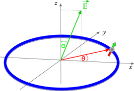
Figure 1: (color online) Sketch of the ring-shaped trap in the $xy$ plane. The dipole moments $\mathbf{d}=d\left(\sin\alpha,0,\cos\alpha\right)$ are aligned by an external field $\mathbf{E}$ in the $xz$-plane.

Let us consider a system of $N$ identical particles (bosons or fermions) of mass $m$ confined in a ring-shaped trap of radius $R$ in the $xy$-plane (Fig. 1). The particles have a dipole moment $\mathbf{d}=d\left(\sin\alpha,0,\cos\alpha\right)$ aligned in the $xz$-plane by an external field, at an angle $\alpha$ to the $z$-axis. The interaction between two dipoles is $V(\mathbf{r})=D^{2}(1-3\cos^{2}\theta_{rd})/r^{3}$, where $\mathbf{r}$ is the separation of the dipoles, $\theta_{rd}$ is the angle between $\mathbf{r}$ and $\mathbf{d}$, and $D^{2}=d^{2}/4\pi\epsilon_{0}$ for electric dipoles and $d^{2}\mu_{0}/4\pi$ for magnetic ones. It is convenient to introduce the length $r_{d}=2mD^{2}/\hbar^{2}$ as a measure of the dipolar interaction. We focus on the limit of a tightly confining ring potential, for which the transverse motion is frozen in the lowest-energy mode, whose spatial extent $a_{\perp}\equiv$$\sqrt{\hbar/m\omega_{\perp}}$ is much smaller than $R$ sinha07 . Integrating out the transverse degrees of freedom, one arrives at an effective 1D Hamiltonian

$$\hat{H}=-\frac{\hbar^{2}}{2mR^{2}}\sum_{i=1}^{N}\frac{\partial^{2}}{\partial\theta_{i}^{2}}+\sum_{i<j}V_{{\rm 1D}}(\theta_{i},\theta_{j}),$$ (1)

where the angle $\theta_{i}$ specifies the position of particle $i$ on the ring. For $R\gg a_{\perp}$, the effective interaction takes the form $V_{{\rm 1D}}(\theta_{1},\theta_{2})=V_{{\rm CM}}\left(\Theta\right)V_{{\rm rel}}(\vartheta)$, where $\Theta=(\theta_{1}+\theta_{2})/2$ is the center-of-mass (CM) angle of the two dipoles and $\vartheta=\theta_{1}-\theta_{2}$ is the relative angle. In terms of the variable $s=2R|\sin(\vartheta/2)|/a_{\perp}$, the dependence on the relative angle is given by dutta06

$$V_{{\rm rel}}(\vartheta)=\sqrt{2\pi}(1+s^{2})e^{s^{2}/2}\mathrm{erfc}(s/\sqrt{2})-2s,$$ (2)

and $V_{{\rm CM}}(\Theta)=D^{2}(1-3\sin^{2}\alpha\sin^{2}\Theta)/4a_{\perp}^{3}$. Thus the CM potential (shown in Fig. 2) has minima at $\Theta=\pm\pi/2$, which become more pronounced as $\alpha$ increases. For $\alpha>\alpha_{\mathrm{c}}\equiv\arcsin(1/\sqrt{3})\approx 0.196\pi$, the potential acquires attractive regions.

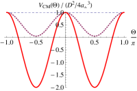
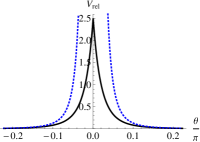
Figure 2: (color online) Left: Coupling strength $V_{{\rm CM}}(\Theta)$ for $\alpha=0$ (dashed), $0.19\pi\approx\alpha_{c}$ (dotted) and ${\pi}/{2}$ (solid). Right: Relative-coordinate potential $V_{{\rm rel}}(\vartheta)$ for $R/a_{\perp}=10$, including the long-range asymptotics (dashed).

Homogeneous interactions —

We first consider the case of dipoles aligned perpendicular to the plane of the ring ($\alpha=0$), for which the interaction is positive and isotropic, and draw some qualitative conclusions before proceeding to the inhomogeneous case. For $\vartheta\to 0$, $V_{{\rm rel}}(\vartheta)$ remains finite because the transverse average cuts off the $1/r^{3}$ divergence of the 3D interaction. Thus for weak enough dipolar repulsion (specified below), the interaction behaves like a potential with range $\sim a_{\perp}$ deuretzbacher09 . For bosonic dipoles, the problem then approximately maps to the Lieb-Liniger model lieb63a on a ring with a contact interaction $g\delta(x_{1}-x_{2})$, where $x_{i}\equiv R\theta_{i}$. For $r_{d}\ll a_{\perp}$, $g$ is the zero-momentum Fourier transform of the potential, and $g=D^{2}/a_{\perp}^{2}$. In the thermodynamic limit $N,R\to\infty$ (keeping the density $n=N/2\pi R$ fixed), the properties of the Lieb-Liniger model are determined by the dimensionless parameter $\gamma=gm/\hbar^{2}n$. For $\gamma\ll 1$ the system is a weakly interacting Bose gas, while for $\gamma\gg 1$ it may be mapped to a noninteracting Fermi gas girardeau60 .

For separations $r\gg a_{\perp}$ the effective 1D interaction behaves as $1/r^{3}$. For sufficiently strong dipolar interaction, this tail becomes important and the system goes over into a crystal-like state, where the dipoles localize as an equally spaced lattice, with energy $E_{{\rm C}}=({ND^{2}}/{16R^{3}})\sum_{\nu=1}^{N-1}\left|\sin[\nu\pi/N]\right|^{-3}$. The amplitude $\Delta$ of the zero-point motion may be estimated to be of order $(\hbar/m\omega)^{1/2}$, where $\omega=(12D^{2}n^{5}/m)^{1/2}$ is the oscillation frequency of a single atom, all others being held fixed. Dipoles are well localized if $\Delta\ll 1/n$, i.e., when the dipole length is large compared with the inter-particle spacing, $(nr_{d})^{1/4}\gg 1$.

Let us now quantify the above considerations. In Fig. 3, we plot the energy of $N=4$ bosonic and fermionic dipoles as a function of interaction strength for $R/a_{\perp}=10$.

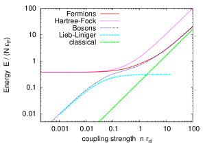
Figure 3: (color online) Homogeneous system ($\alpha=0$): Ground-state energy $E(nr_{d})$ for $N=4$ dipoles. For comparison, the plot includes the Lieb-Liniger results for the Bose gas, Hartree-Fock for fermions, and the classical limit $E_{\mathrm{C}}$.

We see that for $nr_{d}\ll 1$, the bosons are indeed well described by the Lieb-Liniger model with $g=D^{2}/a_{\perp}^{2}$. In particular, for $\gamma=r_{d}/2na_{\perp}^{2}\ll 1$, the bosons form a weakly interacting gas, whereas for $1\lesssim\gamma\ll(na_{\perp})^{-2}$ the bosons tend to fermionize and the energy increases less rapidly with $r_{d}$. For the parameters adopted here, $\gamma=1$ at $nr_{d}=2(na_{\perp})^{2}\approx 0.01$. Note that, since $(na_{\perp})^{2}=nr_{d}/2\gamma$, the fermionized regime is fully separated from the crystal-like one only for strong confinement, $na_{\perp}\ll 1$. For fermions, interaction effects are especially small for $nr_{d}\lesssim 1$ because exchange contributions cancel the direct ones. We also plot the Hartree-Fock energy for comparison.

Inhomogeneous interactions —

For dipoles aligned perpendicular to the plane of the ring, as we discussed above, the system is rotationally invariant about the normal to the plane, and the particle density is uniform. However, for $\alpha\neq 0$ the interaction is smallest for CM angles $\Theta=\pm\pi/2$ and particles tend to lie closer to $\theta=\pm\pi/2$ than to $\theta=0$ or $\pi$. For $nr_{d}\gg 1$, the kinetic energy becomes unimportant, and the configuration is well approximated by particles localized at angles $\theta_{i}$ that minimize the interaction energy.

The upper row in Fig. 4 shows the particle density $\rho(\theta)$ around the ring for $N=4$ bosons (left) and $N=3$ fermions (right) for a dipolar tilt angle $\alpha=0.19\pi$ slightly below the threshold value $\alpha_{c}$. For small couplings $nr_{d}$, the density (green line) reflects the Bose-gas-like state, that gradually develops an inhomogeneity when the interaction is increased to higher values of $nr_{d}$ (blue lines): The initially homogeneous bosonic ground state develops four distinct peaks that demonstrate the localization of the particles near their classical equilibrium positions. The same trend is observed for fermions, as is shown in the right panels of Fig. 4 for $N=3$. For that case, the ground state is a superposition of two states, one of which has two particles near $\theta=\pi/2$ and one near $-\pi/2$, and the other in which the populations are reversed. As a result, the density profile has $2N=6$ peaks rather than $N$.

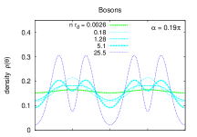
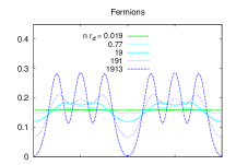
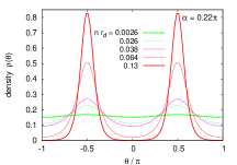
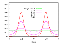
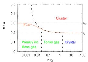
Figure 4: (color online) Density profiles $\rho(\theta)$ for $N=4$ bosons (left) and $N=3$ fermions (right) for $\alpha=0.19\pi$ (uppermost row) and $\alpha=0.22\pi$ (middle row) for different coupling strengths. Bottom: Schematic overview of the different ground states for bosons (for fermions, see text). The dashed lines indicate the boundaries between these approximate regions. On the curved dotted line, the ground-state energy is zero.

For $\alpha>\alpha_{c}$, the interaction is attractive for $\Theta=\pm(\pi/2\pm\Delta\Theta)$ and, for small $\Delta\alpha=\alpha-\alpha_{c}$, $\Delta\Theta\simeq 2^{3/4}\sqrt{\Delta\alpha}$. Then clustered states can be formed, as is illustrated in the middle row of Fig. 4. With increasing interaction strength, the density distribution shows a transition from the homogeneous state to one with two distinct maxima on opposite sides of the ring. This indicates a clustering of the particles due to the attractive part of the interaction, as we further discuss below. The lowest diagram of Fig. 4 summarizes schematically the different ground states for bosons as a function of coupling strength and tilt angle, with the dashed lines indicating the approximate boundaries between the different regimes. The vertical lines corresponds to the values of $nr_{d}$ for which the energy of the Tonks gas equals that of the weakly interacting Bose gas or that of a classical crystal. For fermions, the diagram’s structure is similar, but with the gas-like regions replaced by a single one—a weakly interacting Fermi gas—and clustering occurs at higher $nr_{d}$.

To investigate the clustered states further, we plot in Fig. 5 the ground-state energy of bosons and fermions as a function of the coupling strength for values of $\alpha$ greater than $\alpha_{c}$. The coupling required to produce a bound state is greater for fermions than for bosons for two reasons: first, the Pauli principle leads to a greater kinetic energy for fermions and, second, the exchange hole for fermions reduces the magnitude of the interaction energy.

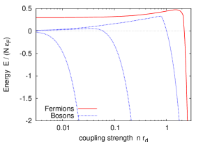
Figure 5: (color online) Ground-state energy $E(nr_{d})$ for $N=3$ fermions (—, $\alpha=0.22\pi$); $N=4$ bosons (- - -, $\alpha=0.2\pi,0.22\pi$, and $\pi/2$ from top to bottom).

With increasing dipole moment, the energy decreases for all $\alpha>\alpha_{c}$ at sufficiently high $nr_{d}$ for both fermions and bosons. For bosons and for $\alpha<\alpha_{c}$, the energy increases monotonically as a function of $nr_{d}$, for $\alpha_{c}<\alpha<\alpha_{c2}\equiv\arcsin\sqrt{2/3}\approx 0.304\pi$ it exhibits a maximum, while for $\alpha>\alpha_{c2}$ it decreases monotonically. The reason for the change in behavior at $\alpha=\alpha_{c2}$ is that, at low densities, the derivative of the energy with respect to density is determined by the spatial average of the two-body interaction, and this changes from positive to negative as $\alpha$ increases through $\alpha_{c2}$. The contribution to the kinetic energy varies as $r_{d}^{2}$ for small $r_{d}$ and is therefore unimportant for weak coupling. For fermions, the energy per particle is always positive for small $r_{d}$ because the Fermi energy dominates the total energy.

Correlations —

We now explore the nature of the ground state in situations where particles are concentrated near $\theta=\pm\pi/2$. Classically, for a repulsive interaction one would expect essentially equal numbers of particles to be present on each side of the ring, while for an attractive interaction, the particles would be concentrated on one side of the ring. A convenient diagnostic for probing the nature of the state is the pair distribution function $\rho_{2}(\theta,\theta^{\prime})=\sum_{i\neq j}\langle\delta(\theta-\theta_{i})\delta(\theta^{\prime}-\theta_{j})\rangle$. For weakly interacting bosons and $0<\alpha<\alpha_{c}$, when the interaction is positive and homogeneous, the system is well described as a Bose–Einstein condensate, with all particles in a single-particle state that has density maxima at the points $\theta=\pm\pi/2$. As shown in Fig. 6, the pair distribution function has maxima in the vicinity of $\theta,\theta^{\prime}=\pm\pi/2$, and they are all of equal strength. For stronger coupling, tunneling between $\theta=\pm\pi/2$ is suppressed, and atoms become localized in the vicinity of $\theta=\pm\pi/2$. In this regime, it is more appropriate to think in terms of Mott-insulator-type states $|N_{+},N_{-}\rangle$ with definite numbers of particles $N_{\pm}$ localized near $\theta=\pm\pi/2$. The ground state for a repulsive interaction would be expected to be dominated by $|N/2,N/2\rangle$, where for simplicity we have taken $N$ to be even. In this case, one expects the peaks around $\theta\approx\theta^{\prime}\approx\pm\pi/2$ to have a strength $1-2/N$ (1/2 for $N=4$) times that of the peaks at $\theta\approx-\theta^{\prime}$. This describes well the data for $nr_{d}=0.803$.

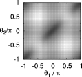
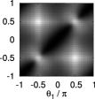
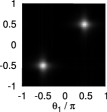
Figure 6: Pair distribution function $\rho_{2}(\theta_{1},\theta_{2})$ for $N=4$ bosons at $\alpha=0.20\pi$ and $nr_{d}=0.026$ (left), $nr_{d}=0.803$ (center) and $nr_{d}=0.808$ (right). Black corresponds to $\rho_{2}=0$ and white to the highest values.

Particles in a bound state would be expected to localize on one side of the ring, in the states $|N,0\rangle$ or $|0,N\rangle$, in order to maximize the attractive contribution to the energy. Because of the symmetry of the system under replacement of $\theta$ by $-\theta$, the ground state will be a linear combination of these states with equal probabilities. For such a state, the pair distribution function is qualitatively different from that of unbound states in that it has only two peaks, at $\theta\approx\theta^{\prime}\approx\pm\pi/2$, as is illustrated in Fig. 6 for $nr_{d}=0.808$, a value only slightly different from the previous one. For very strong coupling $nr_{d}\gg 1$, the critical angle for the formation of bound states approaches $\alpha_{c}$ as is seen in Fig. 4. For weaker coupling, the critical angle for bound state formation increases because of the limited range of CM angles around $\Theta=\pm\pi/2$ for which the interaction is attractive.

Finally, we discuss some experimental aspects. Quasi-1D ring traps with $R/a_{\perp}\sim 10-10^{3}$ and $a_{\perp}\sim 1-10\mu\mathrm{m}$ may be produced using techniques such as time-averaged optical tweezers henderson09 or radiofrequency-dressed magnetic traps sherlock11 . The weak-coupling regime $nr_{d}\ll 1$ may be explored with magnetic atoms (for Cr, $r_{d}\sim 1\mathrm{nm}$), but to observe strong correlations ($\gamma=\pi Rr_{d}/Na_{\perp}^{2}\gg 1$) it is preferable to work with only a small number ($N\sim 10-100$) of molecules and to increase $R/a_{\perp}$. The strongly coupled regime $nr_{d}\gg 1$ may be realized with polar molecules ($r_{d}\sim 0.1\mathrm{\mu m}$ for KRb) and large particle numbers $N\gg 10^{2}R/\mathrm{\mu m}$ (at $\alpha=0$). Measurement of clock shifts similar to those done to determine the atom numbers on sites in the superfluid-insulator transition campbell would be a useful way to distinguish between the state $|N/2,N/2\rangle$ and Schrödinger-cat-like states that are superpositions of $|N,0\rangle$ and $|0,N\rangle$.

In conclusion, we have shown that dipolar particles in ring traps may be used to realize a variety of different states due to the interplay between the ring geometry, dipolar anisotropy, and confinement. This includes both inhomogeneously localized states as well as unconventional effective short-range physics, which may be explored by tuning the numbers of dipolar atoms or molecules, their orientation, and the trapping parameters.

We thank J. Cremon, F. Deuretzbacher, M. Girardeau, A. Griesmaier, and H.-D. Meyer for discussions. SZ was supported by the German Academy of Sciences Leopoldina (LPDS 2009-11). Part of this work was supported by the Swedish Research Council.

- (1) T. Lahaye et al., Nature 448, 672 (2007); T. Koch et al., Nat. Phys. 4, 218 (2008); J. Deiglmayr et al., Phys. Rev. Lett. 101, 133004 (2008); K.-K. Ni et al., Science 322, 231 (2008); S. Ospelkaus et al., ibid. 327, 853 (2010); Phys. Rev. Lett. 104, 30402 (2010); M. Lu, S. H. Youn, and B. L. Lev, ibid. 104, 063001 (2010); K.-K. Ni et al., Nature 464, 1324 (2010).
- (2) M. A. Baranov, Phys. Rep. 464, 71 (2008).
- (3) T. Lahaye et al., Rep. Prog. Phys. 72, 126401 (2009).
- (4) G. Bruun and E. Taylor, Phys. Rev. Lett. 101, 245301 (2008); N. Cooper and G. Shlyapnikov, Phys. Rev. Lett. 103, 155302 (2009).
- (5) See, e.g., R. Citro et al., Phys. Rev. A 75, 51602(R) (2007); T. Roscilde and M. Boninsegni, New J. Phys. 12, 033032 (2010).
- (6) A. S. Arkhipov et al., JETP Lett. 82, 39 (2005).
- (7) O. Dutta, M. Jääskeläinen, and P. Meystre, Phys. Rev. A 73, 043610 (2006).
- (8) D. Bauer et al., Nature Phys. 5, 339 (2009).
- (9) For bosons, a similar system has recently been considered in the Gross–Pitaevskii approximation, M. Abad et al., Phys. Rev. A 81, 043619 (2010).
- (10) K. Henderson et al., New J. Phys. 11, 043030 (2009); A. Ramanathan et al., Phys. Rev. Lett. 106, 130401 (2011).
- (11) B. E. Sherlock et al., Phys. Rev. A 83, 043408 (2011).
- (12) S. Viefers et al., Physica E 21, 1 (2004).
- (13) M. H. Beck et al., Phys. Rep. 324, 1 (2000); for its application to cold atoms, see, e.g., S. Zöllner, H.-D. Meyer, and P. Schmelcher, Phys. Rev. A 74, 053612 (2006).
- (14) We neglect virtual excitation of higher transverse modes, which would alter the 1D effective interaction olshanii98 , see S. Sinha and L. Santos, Phys. Rev. Lett. 99, 140406 (2007).
- (15) F. Deuretzbacher, J. C. Cremon, and S. M. Reimann, Phys. Rev. A 81, 063616 (2010).
- (16) E. H. Lieb and W. Liniger, Phys. Rev. 130, 1605 (1963).
- (17) M. Girardeau, J. Math. Phys. 1, 516 (1960).
- (18) G. K. Campbell et al., Science 313, 649 (2006).
- (19) M. Olshanii, Phys. Rev. Lett. 81, 938 (1998).