High fidelity quantum gates via dynamical decoupling

Abstract

Realizing the theoretical promise of quantum computers will require overcoming decoherence. Here we demonstrate numerically that high fidelity quantum gates are possible within a framework of quantum dynamical decoupling. Orders of magnitude improvement in the fidelities of a universal set of quantum gates, relative to unprotected evolution, is achieved over a broad range of system-environment coupling strengths, using recursively constructed (concatenated) dynamical decoupling pulse sequences.

Introduction.—Quantum systems are famously susceptible to interactions with their surrounding environments, a process which leads to a progressive loss of “quantumness” of these systems, via decoherence Zurek (1991). When a system performs a quantum information processing (QIP) task this loss of quantumness is equivalent to the accumulation of computational errors, which leads to the eventual loss of any quantum advantage in information processing. Robust large-scale quantum information processing therefore requires that decoherence—or any otherwise undesired evolution—of a quantum state be minimized to the largest extent possible by clever system choice and engineering. One may then hope to apply the powerful techniques of fault tolerant quantum error correction (FT-QEC) Gaitan (2008). However, FT-QEC imposes significant resource requirements, in particular rapidly growing spatial and temporal overhead, together with demanding gate and memory error rates which must remain below a certain threshold (e.g., Refs. Aliferis et al. (2006)). This motivates the search for alternative strategies which can slow down decoherence and “keep quantumness alive.” Dynamical decoupling (DD) is a form of quantum error suppression that modifies the system-environment interaction so that its overall effects are very nearly self-canceling, thereby decoupling the system evolution from that of the noise-inducing environment Viola et al. (1999a). DD has primarily been studied as a specialized control technique for quantum memory (i.e., arbitrary state preservation) Viola and Knill (2005); Khodjasteh and Lidar (2005); Witzel and Das Sarma (2007); Zhang et al. (2008); Uhrig (2007); Yang and Liu (2008); West et al. (2009); UL:10 , as convincingly demonstrated by a number of recent experiments in QIP platforms as diverse as electron-nuclear systems Li et al. (2007); Du et al. (2009), photonics qubits Damodarakurup et al. (2009), and trapped ions Biercuk et al. (2009). However, the holy grail of QIP is not just to store states robustly, but rather to perform universal computation robustly Nielsen and Chuang (2000). Fortunately, there are abstract results showing that DD is in principle compatible with computation, essentially by designing DD operations that commute with the computational operations Viola et al. (1999b). Additionally, recent theoretical results indicate that high fidelity “dynamically error-corrected gates” can be designed, using methods inspired by DD Khodjasteh and Viola (2009), and that DD can be merged with FT-QEC to reduce resource overhead, or even improve gate error rates to below threshold Ng et al. (2009). DD can also be used to improve the fidelity of adiabatic quantum computation D. A. Lidar (2008). Experimentally, DD has been successfully combined with QEC in nuclear spin systems to demonstrate robust quantum memory N. Boulant, M.A. Pravia, E.M. Fortunato, T.F. Havel and D.G. Cory (2002). In principle, then, it appears that DD is a suitable control technique for overcoming decoherence and improving gate fidelity. However, a very practical question still remains: what are the conditions under which DD can be used to perform universal quantum computation with a given fidelity? Recent rigorous bounds devised for the popular “periodic DD” (PDD) protocol suggest that it is severely limited in this regard Khodjasteh and Lidar (2008). Here we demonstrate, using numerical simulations of a logical qubit coupled to a small bath, that recursively constructed, concatenated DD (CDD) pulse sequences Khodjasteh and Lidar (2005), can be used to endow a universal set of quantum logic gates with remarkably high fidelities. Though our numerical results illustrate the effectiveness of CDD in a model inspired by quantum dot implementations of QIP Burkard:99 , the framework we describe is in principle more generally applicable, provided encoding and encoded gates can be implemented. We therefore expect that our results will contribute to establishing DD as an indispensable tool in scalable QIP.

Dynamical decoupling.—The total Hamiltonian without DD is $H=H_{B}+H_{SB}$, where $H_{B}$ includes all bath-only terms and $H_{SB}$ includes all terms acting non-trivially on the system. To suppress error, DD allows the joint evolution to proceed under $H$ for some time before applying a control pulse $P_{j}$ to the system alone [generated by a time-dependent system-only Hamiltonian $H_{S}(t)$ which is added to $H$], designed to refocus the evolution toward the error-free ideal, continually repeating this process until some total evolution has been completed: $\operatorname{DD}[U(\tau_{0})]=P_{N}U(\tau_{0})\cdots P_{2}U(\tau_{0})P_{1}U(\tau_{0})\equiv\widetilde{U}(N\tau_{0})$, where $U(\tau_{0})=U_{0}(\tau_{0})B(\tau_{0})$ represents the joint system-bath unitary evolution generated by $H$, for a duration of length $\tau_{0}$ (the pulse interval), decomposed so that $U_{0}(\tau_{0})$ determines the ideal, desired system-only error-free evolution, and $B(\tau_{0})$ is a unitary error operator acting jointly on the system and bath. Here and below we use a tilde to denote evolution in the presence of DD pulses. DD schemes with non-uniform pulse intervals have also been considered and shown to be very powerful for quantum memory purposes Uhrig (2007); Yang and Liu (2008); West et al. (2009); UL:10 ; Biercuk et al. (2009); Du et al. (2009), but since it is unclear how to use them for computation involving multiple qubits, we shall limit our discussion to uniform-interval schemes. For now, but not in our simulations presented below, we assume for simplicity of presentation that the pulses $\{P_{j}\}$ are sufficiently fast as to not contribute to the total time of the evolution. The simplest example is quantum memory, where $U_{0}(\tau_{0})=I_{S}$ is the identity operation, and $B(\tau_{0})$ represents the deviation from the ideal dynamics caused by the presence of a bath. In this case, our goal is to choose pulses so that $\operatorname{DD}[U(\tau_{0})]=I_{S}\otimes\widetilde{B}$, where $\widetilde{B}$ is an arbitrary pure-bath operator. Uniform-interval DD schemes differ in precisely how the pulses $\{P_{j}\}$ are chosen, with the only common constraint that the following basic “decoupling condition” (vanishing average Hamiltonian, i.e., vanishing first order term in the Magnus series of the joint system-bath evolution) is met Viola et al. (1999a): $\sum_{\alpha}P_{\alpha}^{{\dagger}}H_{SB}P_{\alpha}=0$. To be concrete, we will suppose that the pulses $P_{\alpha}\in\{I,X,Y,Z\}$ are Pauli operators. CDD generates pulse sequences by recursively building on a base sequence $Z[\cdot]X[\cdot]Z[\cdot]X[\cdot]$ (motivated below), where $[\cdot]$ denotes either free evolution or the insertion of gate operations between pulses. The sequence is initialized as $\operatorname{CDD}_{0}[U(\tau_{0})]=U(\tau_{0})=U_{0}(\tau_{0})B(\tau_{0})\equiv\widetilde{U}_{0}(\tau_{0})$, and higher levels are generated via the rule $\operatorname{CDD}_{n+1}[U(\tau_{0})]=Z[\widetilde{U}_{n}(\tau_{n})]X[\widetilde{U}_{n}(\tau_{n})]Z[\widetilde{U}_{n}(\tau_{n})]X[\widetilde{U}_{n}(\tau_{n})]\equiv\widetilde{U}_{n+1}(\tau_{n+1})$, where $\tau_{n}=4^{n}\tau_{0}$. Note that in contrast to previous work on CDD Khodjasteh and Lidar (2005); Witzel and Das Sarma (2007); Ng et al. (2009), we are allowing for the possibility of some non-trivial information processing operation $U_{0}(\tau_{0})$, as this will be required in our discussion of universal computation below. The choice of the base sequence is motivated by the observation that it satisfies the “decoupling condition”, in the quantum memory setting $U_{0}(\tau_{0})=I_{S}$, under the dominant “1-local” system-bath coupling term $H_{SB}^{(1)}=\sum_{\alpha\in\{x,y,z\}}\sum_{j}\sigma_{j}^{\alpha}\otimes B_{j}^{\alpha}$, where $\sigma_{j}^{x}\equiv X$, $\sigma_{j}^{y}\equiv Y$, and $\sigma_{j}^{z}\equiv Z$ denote the Pauli matrices acting on system qubit $j$, and $\{B_{j}^{\alpha}\}$ are arbitrary bath operators. (The next order “2-local” coupling would have terms such as $\sigma_{j}^{\alpha}\sigma_{k}^{\beta}\otimes B_{jk}^{\alpha\beta}$, etc.) Similarly, the most common pulse sequence used thus far in DD experiments (e.g., Refs. N. Boulant, M.A. Pravia, E.M. Fortunato, T.F. Havel and D.G. Cory (2002); Li et al. (2007)) is PDD, which generates pulse sequences by periodically repeating the base sequence $Z[\cdot]X[\cdot]Z[\cdot]X[\cdot]$: $\operatorname{PDD}_{k}[U(\tau_{0})]=(\operatorname{PDD}_{1}[U(\tau_{0})])^{k}=\widetilde{U}_{k}(4k\tau_{0})$, where $\operatorname{PDD}_{1}[U(\tau_{0})]=\operatorname{CDD}_{1}[U(\tau_{0})]$. Rigorous noise reduction bounds are known for both PDD and CDD in the quantum memory setting, and show that CDD is a much more effective strategy than PDD, provided $(\left\|H_{B}\right\|+\left\|H_{SB}\right\|)\tau_{0}$ is sufficiently small, where the norm is the largest eigenvalue Ng et al. (2009). It is convenient to characterize the leading-order DD behavior in terms of $\left\|H_{B}\right\|$ and $\left\|H_{SB}\right\|$, as these parameters capture the strength or overall rate of the internal bath and system-bath dynamics, respectively. If $\left\|H_{SB}\right\|\gg\left\|H_{B}\right\|$, then the system-bath coupling is a dominant source of error. In this case, DD should produce significant fidelity gains as it removes the dominant error source. On the other hand, if $\left\|H_{SB}\right\|<\left\|H_{B}\right\|$, then the system-bath coupling induces relatively slow dynamics, while the environment itself has fast internal dynamics. In this case, suppressing the system-bath coupling will have less of an effect on the overall dynamics, so it may be considered a worst case scenario when assessing DD performance.

High fidelity universal quantum gates using CDD.— Our main goal in this work is to demonstrate that we can generate a universal set of logic gates which is highly robust in the presence of a decohering environment. As a model system we consider electron spin qubits in semiconductor quantum dots Burkard:99 , which we study numerically via full-quantum-state (sometimes called “numerically exact”) simulations over a wide range of system-bath coupling parameters. In such systems the dominant bath is provided by the nuclear spins Witzel and Das Sarma (2007), and the interaction between system and environment is described by a Heisenberg exchange Hamiltonian with exponentially decreasing strength as a function of distance $d_{ij}$ between system qubit $j$ and bath qubit $i$. Thus, we let $B_{j}^{\alpha}=J\sum_{i}\sigma_{i}^{\alpha}/2^{d_{ij}}$ in the system-bath Hamiltonian $H_{SB}^{(1)}$, so that $\left\|H_{SB}\right\|\propto J$. We model the interaction between the bath nuclear spin qubits as dipole-dipole coupling, i.e., $H_{B}=\beta\sum_{i<j}\left(\sigma_{i}^{y}\sigma_{j}^{y}+\sigma_{i}^{z}\sigma_{j}^{z}-2\sigma_{i}^{x}\sigma_{j}^{x}\right)/d_{ij}^{3}$ so that $\left\|H_{B}\right\|\propto\beta$, where now $d_{ij}$ is the distance between bath qubits $i$ and $j$. In our simulations we pick the parameters $J$, $\beta$, and $d_{ij}$, as well as the pulse interval $\tau_{0}$ and the pulse width, to include a range of interest for GaAs and Si quantum dots Petta ; supp-mat . The $H_{SB}$ and $H_{B}$ Hamiltonians are on during the entire pulse sequence execution, while $H_{S}(t)$ pulses appropriately between dynamical decoupling ($H_{S}=H_{DD}$) and computational operations ($H_{S}=H_{G}$).

Universal quantum computation requires that only a discrete set of universal gates be implemented; a particularly simple choice are the Hadamard, $\pi/8$, and controlled-phase gates Nielsen and Chuang (2000). The first two are single-qubit gates, and the third is a two-qubit gate which can be used to generate entanglement. A conundrum immediately presents itself when trying to combine computation with DD: how to make sure that the DD pulses do not cancel the (system Hamiltonian implementing the) gates? One solution is to use an encoding so that the DD operations commute with the logical gate operations Viola et al. (1999b); D. A. Lidar (2008); Byrd and Lidar (2002). To this end we use logical qubits encoded into a four-qubit decoherence-free subspace (DFS). The logical basis states are the two orthonormal total spin-zero states of four spin-$1/2$ particles, first described as a DFS in Ref. Zanardi and Rasetti (1997). We stress that our system-bath interaction does not exhibit any symmetries so that there is no naturally occuring DFS which can be used to store protected quantum information; instead, our encoding choice is motivated by the fact that in this setting, a universal set of encoded computational operations can be generated by controllable Heisenberg exchange Hamiltonians between the system qubits ($=H_{G}$), as first described in Bacon et al. (2000), and these commute with the global Pauli operations $\left\{\bar{X},\bar{Z}\right\}=\left\{X_{1}X_{2}X_{3}X_{4},Z_{1}Z_{2}Z_{3}Z_{4}\right\}$ used as decoupling pulses. To generate these pulses $H_{DD}$ is modeled as a controllable uniform magnetic field. However, we emphasize that these choices are by no means unique. Any choice of DD pulses $\{P_{j}\}$ such that $[H_{G},P_{j}]=0$ $\forall j$ will suffice Viola et al. (1999b), including, e.g., the stabilizer quantum error correcting codes relevant in the theory of FT-QEC used as DD pulses, and the normalizers of these codes used to generate computational gates Byrd and Lidar (2002); D. A. Lidar (2008).

Faced with several options for combining DD and computational operations Viola et al. (1999b); Khodjasteh and Lidar (2008), we chose the following “decouple while compute” strategy. In this strategy we alternate between applying computational and DD operations, thus spreading a computational gate over the entire CDD pulse sequence. We do this by applying the $N^{\mathrm{th}}$ root of the gate $N$ times during a CDD pulse sequence involving $N=4^{n}$ pulses. Thus, if the ideal computational gate is $G(T)=e^{-iH_{G}T}$, we implement it by applying $U(\tau_{0})=e^{-i(H_{G}+H_{SB}+H_{B})\tau_{0}}$ between each of the $N$ pulses, where $\tau_{0}=T/N$. As $T$ increases with concatenation level $n$, the exchange couplings in $H_{G}$ are proportionately decreased so that the $\|H_{G}\|T$ product remains constant; in all simulations the pulse interval $\tau_{0}$ is held fixed at 1ns, the time-scale for exchange operations in semiconductor quantum dots Petta . This “decouple while compute” strategy is precisely the formulation presented in the expressions for $\operatorname{CDD}_{n+1}[U(\tau_{0})]$ and $\operatorname{PDD}_{k}[U(\tau_{0})]$ above, provided we identify $U_{0}(\tau_{0})B(\tau_{0})$ there with $U(\tau_{0})$ here, and $U_{0}(\tau_{0})$ there with $G(\tau_{0})$ here. Other strategies are certainly also conceivable, e.g., a “decouple then compute” strategy wherein $U_{0}(\tau_{0})$ is simply the identity operation, and the gate is implemented at the end of the pulse sequence. While the latter strategy was shown to be capable of reducing the resource requirements of FT-QEC Ng et al. (2009), we found in our simulations that we obtain a higher fidelity when we use “decouple while compute”, because then time is not wasted on free evolution during the intervals between pulses.

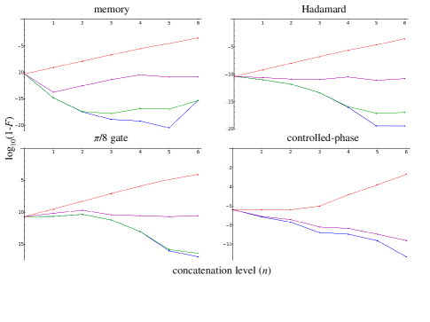
Figure 1: (color online) Fidelity of a universal set of encoded gates under CDD. The coupling strengths and bath dynamics are determined by the parameters $J=10$kHz and $\beta=1$MHz, respectively (we work in units of $\hbar=1$). Pulse intervals are fixed at $\tau_{0}=1$ns, while pulse widths are given by $\delta=0$, $\delta=1$ps, and $\delta=1$ns, corresponding, from bottom to top, to the blue, green (absent for controlled-phase), and magenta lines, respectively. The red dashed line shows the unprotected evolution over a time period $T=4^{n}\tau_{0}$. Notice that the $\log_{10}(1-F)$ ranges change between plots. Also, $n=0$ corresponds to free evolution for a duration $\tau_{0}=1$ns, whence the $n=0$ point starts at a relatively high fidelity. Results depend only slightly on the choice of initial system state.

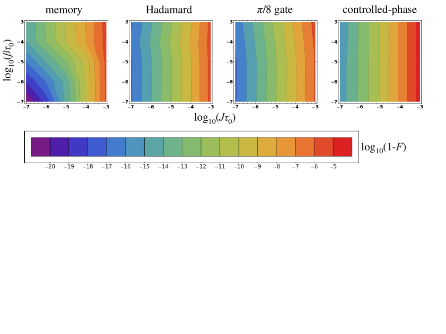
Figure 2: (color online) Constant fidelity contours for the system described in the previous figure, at fixed concatenation level $n=5$ and pulse width $\delta=1$ns. Notice that the fidelity contours are strongly dependent on $J\tau_{0}$.

We now present our simulation results (details of the numerical procedure are given in supp-mat ). The worst-case scenario of $J<\beta$ is shown in Fig. 1 , where we plot $\log_{10}(1-F)$ vs. concatenation level for each of the universal gates, with the fidelity defined as $F\equiv\sqrt{|\left\langle\psi\right|\rho\left|\psi\right\rangle|}$, where $\rho$ is the mixed output system state (obtained from the joint system-bath evolution after partial trace over the bath) and $\left|\psi\right\rangle$ is the desired system state. In each of these plots, the red dashed line represents undecoupled free evolution for increasing total time, given by $T=4^{n}\tau_{0}$. As the evolution time increases, error accumulates and fidelity correspondingly worsens, while $\operatorname{CDD}_{n}$ combats this effect with each successive level of concatenation. To contrast, the blue line in these graphs shows $\operatorname{CDD}_{n}$ with ideal, zero-width DD pulses, so that realistic, finite-width DD pulses lie somewhere between the blue and red lines, as shown. In each of the plots in Fig. 1 CDD achieves impressive results, even when pulse widths are as long as the intervals, that is, when $\delta=\tau_{0}=1$ns as depicted with the magenta lines, CDD still manages more than five orders of magnitude improvement in fidelity over free evolution. As the pulse width $\delta$ narrows relative to the pulse interval $\tau_{0}$, that is, as the DD pulses becomes faster, fidelity improvement grows to between ten and twenty orders of magnitude over free evolution.

The results for the encoded $\pi/8$ and Hadamard gates are similar, which is not surprising given that they require, respectively, one and two elementary Heisenberg exchange operations to be implemented Bacon et al. (2000); Bacon (2001). The fidelity of the controlled-phase gate is several orders of magnitude lower, which is due to the fact that it involves a much longer sequence of $42$ elementary Heisenberg operations Bacon (2001). Finally, while the quantum memory results are comparable to those of the Hadamard and $\pi/8$-gates, we attribute the reduction in memory fidelity at the highest concatenation level to the absence of $H_{G}$ during the intervals between pulses. Indeed, having the system Hamiltonian “on” during the pulse intervals has a beneficial effect, as it effectively reduces the strength of the bath and system-bath Hamiltonians. The overall conclusion from Fig. 1 is rather encouraging: it appears to be possible to implement a universal set of quantum logic gates with a high fidelity in the presence of coupling to a spin bath.

The results in Fig. 1 are for specific coupling parameters chosen deliberately to represent a worst-case scenario for DD, in that $J<\beta$. As we next demonstrate, the conclusions are robust: CDD remains effective over a broad range of bath dynamics and system-bath coupling strengths. Figure 2 shows the resilience of CDD to widely varying environments by displaying constant fidelity contours in $(J\tau_{0},\beta\tau_{0})$ space, at fixed concatenation level and pulse width, as indicated. Note that fixing $n$ and $\delta$ renders the total evolution time constant, so that fidelity becomes strictly a function of the dimensionless coupling parameters $(J\tau_{0},\beta\tau_{0})$. These plots show a strong fidelity dependence on $J\tau_{0}$, and a very weak dependence on $\beta\tau_{0}$, except in the quantum memory case.

More generally, our results show that CDD is effective over a broad range of coupling parameters, including the fundamentally different “good” ($J>\beta$) and “bad” ($J<\beta$) regimes. This conclusion is further bolstered by our complete gate fidelity simulations supp-mat , where the $\beta$ and $J$ parameters each vary over the range from $1$Hz to $1$MHz. In these simulations the non-memory gate fidelities improve monotonically as a function of concatenation level for all values of $J$ and $\beta$. Taken in their totality, our simulation results indicate that universal quantum computation can be combined with CDD to achieve very high fidelities.

Discussion.—The high gate fidelities we have reported here suggest that it is advantageous to incorporate CDD as a first layer of defense against decoherence, in a more complete FT-QEC scheme. In this regard our “decouple while compute” study complements the “decouple then compute” strategy for which it has already been shown that incorporating DD, and in particular CDD, into FT-QEC can lead to substantial improvements Ng et al. (2009). It will be interesting to determine which strategy leads to better performance overall. Undoubtedly, optimal control methods will offer important additional performance improvements in the implementation of encoded logic gates Cappellaro et al. (2006). We look forward to experimental tests of CDD-protected quantum memory and logic gates.

The views and conclusions contained in this document are those of the authors and should not be interpreted as representing the official policies, either expressly or implied, of the United States Department of Defense or the U.S. Government. Approved for public release, distribution unlimited.

Acknowledgments.— All authors were sponsored by the United States Department of Defense. D.A.L. was also sponsored by NSF under Grants No. CHM-924318, CCF-726439 and PHY-803304.

Appendix A The DFS code

We describe the four-qubit DFS code, first proposed in the context of providing immunity against collective decoherence processes Zanardi and Rasetti (1997). Let $S$ and $m_{S}$ denote the quantum numbers associated with total spin and its projection, and let the singlet and triplet states of two electrons $i,j$ be denoted as

$$|s\rangle_{ij}\equiv|S=0,m_{S}=0\rangle=\frac{1}{\sqrt{2}}\left(|\Psi(\uparrow\downarrow)\rangle-|\Psi(\downarrow\uparrow)\rangle\right)$$

$$|t_{-}\rangle_{ij}\equiv|S=1,m_{S}=-1\rangle=|\Psi(\downarrow\downarrow)\rangle$$

$$|t_{0}\rangle_{ij}\equiv|S=1,m_{S}=0\rangle=\frac{1}{\sqrt{2}}\left(|\Psi(\uparrow\downarrow)\rangle-|\Psi(\downarrow\uparrow)\rangle\right)$$

$$|t_{+}\rangle_{ij}\equiv|S=1,m_{S}=1\rangle=|\Psi(\uparrow\uparrow)\rangle.$$

Here $|\Psi(\downarrow\uparrow)\rangle$ denotes a normalized basis state with the first (second) electron in the spin up (down) state, etc. Then a single encoded DFS qubit is formed by the two singlets of four spins, i.e., the two states with zero total spin $S_{\mathrm{T}}=\left|\mathbf{S}_{A}+\mathbf{S}_{B}+\mathbf{S}_{C}+\mathbf{S}_{D}\right|$, where $\mathbf{S}_{i}$ is the Pauli spin vector-operator of electron $i$. These states are formed by combining two singlets of two pairs of spins ($|0_{L}\rangle$), or triplets of two pairs of spins ($|1_{L}\rangle$), with appropriate Clebsch-Gordan coefficients:

$$|0_{L}\rangle = |s\rangle_{AB}\otimes|s\rangle_{CD}$$

$$= \frac{1}{2}\left(|\Psi(\uparrow\downarrow\uparrow\downarrow)\rangle+|\Psi(\downarrow\uparrow\downarrow\uparrow)\rangle-|\Psi(\uparrow\downarrow\downarrow\uparrow)\rangle-|\Psi(\downarrow\uparrow\uparrow\downarrow)\rangle\right)$$

$$|1_{L}\rangle = \frac{1}{\sqrt{3}}\left(|t_{-}\rangle_{AB}\otimes|t_{+}\rangle_{CD}-|t_{0}\rangle_{AB}\otimes|t_{0}\rangle_{CD}+|t_{+}\rangle_{AB}\otimes|t_{-}\rangle_{CD}\right)$$

$$= \frac{1}{\sqrt{3}}(2|\Psi(\uparrow\uparrow\downarrow\downarrow)\rangle+2|\Psi(\downarrow\downarrow\uparrow\uparrow)\rangle-|\Psi(\uparrow\downarrow\downarrow\uparrow)\rangle-|\Psi(\downarrow\uparrow\uparrow\downarrow)\rangle-|\Psi(\uparrow\downarrow\uparrow\downarrow)\rangle-|\Psi(\downarrow\uparrow\downarrow\uparrow)\rangle).$$

The details of the sequences of exchange interactions needed to implement the Hadamard, $\pi/8$, and controlled-phase gates over this DFS code are too long to give here. However, they have been well documented in the original works Bacon et al. (2000); Kempe et al. (2001); Bacon (2001), and perhaps most concisely in the more recent Ref. Woodworth et al. (2005).

Appendix B Details of the numerical procedure

We performed numerically exact simulations since we required extremely high precision fidelity results, inaccessible via approximation techniques Witzel and Sarma (2006); Yang and Liu (2008) capable of handling much larger system and bath sizes. Such methods are required for long time scale simulations, which is not our case. Moreover, large-scale simulations Witzel and Das Sarma (2007) have confirmed earlier small-bath simulations of CDD pulse sequences Khodjasteh and Lidar (2005, 2007). Our numerically exact simulations ran at 100-200 digits of numerical precision, for more than 90 hours on a computer with a dual core intel processor (2GHz + 2G RAM). In our simulations, each logical qubit was encoded using four physical qubits. We tested for dependence on the initial encoded system state, and found a variation in output fidelity of less than an order of magnitude. Hence all our reported results are for the logical-one initial state. As a further test we considered several simple bath geometries: linear, circular, and polygonal. Our results did not depend appreciably on this geometry. We took the initial bath state as the uniform superposition, zero temperature state $\frac{1}{\sqrt{B}}\sum_{i=1}^{B}\left|i\right\rangle$, where $B=2^{N_{n}}$ is the number of available pure bath states when $N_{n}$ bath qubits are present. We checked that finite temperature has only a small quantitative effect on our reported fidelities. In order to keep our numerically exact simulations feasible we had to restrict the total number of qubits to ten, and hence the size of the bath to only two physical qubits when considering two encoded 4-qubit DFS qubits. For consistency we also used two bath qubits in our single encoded qubit simulations. However, we adjusted the strength of the coupling to the bath to account for this, using a scaling relation we found by testing bath sizes in the range $2\leq N_{n}\leq 5$. While we are fully aware of the potential problems associated with using a small bath at long time scales, we expect our small bath simulations to be reliable, as we are concerned only with short timescales, relative to the magnitudes of $J$ and $\beta$, so that possible coherence recurrences due to non-Markovian effects are well out of reach.

Appendix C Complete simulation results

Figures 3-8 present our complete gate fidelity results for the 4-qubit DFS code subject to free evolution or CDD, with the $\beta$ and $J$ parameters each varying over the range from 1Hz to 1MHz. The pulse interval $\tau_{0}$ is fixed at 1ns, and the pulse width assumes the values 0, 1ps, and 1ns. In all cases CDD leads to a fidelity improvement of many orders of magnitude relative to free evolution. The plots surrounded by dashed line boxes are the ones shown in Fig. 1 in the main text.

Appendix D GaAs and Si parameters

We picked the ranges of our $\beta$ and $J$ parameters shown in Figs. 3-8 to represent realistic quantum dot systems – see Table 1. The $J$ parameters in this table were estimated directly from the contact hyperfine interaction between a quantum dot electron and nuclear spins. For GaAs the hyperfine constant is $A=90\mu$eV Coish et al. (2006). For polarized nuclei, the interaction strength is reduced by the number of nuclei $N_{n}$, typically in the range $10^{5}$ to $10^{6}$ per quantum dot, giving $J=A/N_{n}$. For unpolarized nuclei, the interaction strength is reduced by $\sqrt{N_{n}}$ Coish et al. (2006). For Si (silicon), the contact hyperfine strength $A$ is computed from $A=\frac{8\pi}{3}\mu_{{}^{29}Si}\mu_{B}r\nu\eta$, where $\mu_{j}$ is the nuclear or electron (Bohr) magnetic moment, $r$ is the fraction of non-zero spin ²⁹Si nuclei, $\nu$ is the Si nuclear number density, and $\eta$ is the concentration of the electron Bloch wavefunction near the Si nuclei Hale and Mieher (1959). For natural abundance Si we obtained $A=60$neV. For polarized nuclei, the interaction strength is reduced by the number $N_{n}\sim 6\times 10^{4}$ of ²⁹Si in a quantum dot. For unpolarized nuclei the interaction strength is again reduced by $\sqrt{N_{n}}$.

For both GaAs and Si the energy scale $\beta$ of the bath is taken to be $1/T_{2n}$, the inverse of the nuclear dephasing time. For GaAs, the nuclear dephasing time has been estimated at $T_{2n}=100\mu$s Khaetskii et al. (2002); Merkulov et al. (2002), which is the precession time of a nucleus in the dipole magnetic field generated by neighboring nuclei. For Si, the nuclear dephasing time has been measured to be $T_{2n}=5.6m$s Dementyev et al. (2003), again corresponding to the evolution time due to the dipole-dipole interaction between a ²⁹Si nucleus and neighboring ²⁹Si nuclei.

Table 1
system	$J$	$\beta$
unpolarized GaAs	$100$MHz	$10$kHz
polarized GaAs	$1$MHz	$10$kHz
unpolarized Si	$400$kHz	$180$Hz
polarized Si	$1.5$kHz	$180$Hz

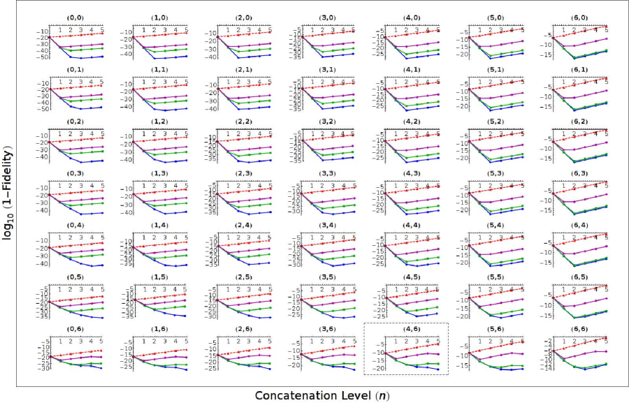
Figure 3: CDD quantum memory in the 4-qubit DFS encoding with pulse interval $\tau_{0}=10^{-9}s$, and pulse widths $\delta=0$s, $\delta=10^{-12}$s, and $\delta=10^{-9}$s corresponding to the blue, green, and magenta lines, respectively. The dashed-red represents free evolution without DD for increasing total times $T=4^{n}\tau_{0}$. The plots are labeled by the strength of the coupling parameters $(\log_{10}J,\log_{10}\beta)$, in Hz. Thus $J$ increases in strength in multiples of $10$ from left to right, and $\beta$ similarly increases from top to bottom. Notice that the $\log_{10}(1-\text{Fidelity})$ ranges change between plots.

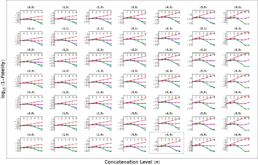
Figure 4: Same as Figure 3, for the $\pi/8$ gate.

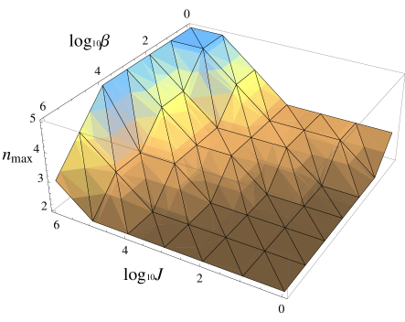
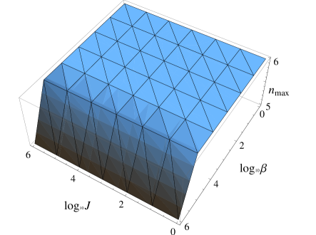
Figure 5: Top: Turning point of the memory fidelity shown in Figure 3, i.e., the maximum concatenation level before fidelity decreases, as a function of $\log_{10}J$ and $\log_{10}\beta$, in Hz. Bottom: Same for the $\pi/8$ gate fidelity shown in Figure 4.

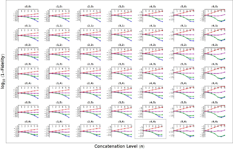
Figure 6: Same as Figure 3, for the Hadamard gate.

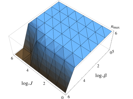
Figure 7: Turning point of the Hadamard gate fidelity shown in Figure 6, i.e., the maximum concatenation level before fidelity decreases, as a function of $\log_{10}J$ and $\log_{10}\beta$, in Hz. Note that slightly better performance is obtained for the $\pi/8$ gate. This is due to the fact that it takes only a single elementary Heisenberg exchange operation to implement, while the Hadamard gate takes two such operations, i.e., double the time.

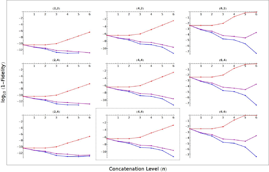
Figure 8: Same as Figure 3, for the controlled-phase gate.

References

- Zurek (1991) W. Zurek, Physics Today 44, 36 (1991).
- Gaitan (2008) F. Gaitan, Quantum Error Correction and Fault Tolerant Quantum Computing (CRC, Boca Raton, 2008).
- Aliferis et al. (2006) P. Aliferis, D. Gottesman, and J. Preskill, Quantum Inf. Comput. 6, 97 (2006); E. Knill, Nature 434, 39 (2005).
- Viola et al. (1999a) L. Viola, E. Knill, and S. Lloyd, Phys. Rev. Lett. 82, 2417 (1999a); P. Zanardi, Phys. Lett. A 258, 77 (1999).
- Viola and Knill (2005) L. Viola and E. Knill, Phys. Rev. Lett. 94, 060502 (2005).
- Khodjasteh and Lidar (2005) K. Khodjasteh and D. A. Lidar, Phys. Rev. Lett. 95, 180501 (2005); K. Khodjasteh and D. A. Lidar, Phys. Rev. A 75, 062310 (2007).
- Witzel and Das Sarma (2007) W. M. Witzel and S. Das Sarma, Phys. Rev. B 76, 241303(R) (2007).
- Zhang et al. (2008) W. Zhang et al., Phys. Rev. B 77, 125336 (2008).
- Uhrig (2007) G.S. Uhrig, Phys. Rev. Lett. 98, 100504 (2007).
- Yang and Liu (2008) W. Yang and R.-B. Liu, Phys. Rev. Lett. 101, 180403 (2008).
- West et al. (2009) J. R. West, B. H. Fong, and D. A. Lidar, Phys. Rev. Lett. 104, 130501 (2010).
- (12) G.S. Uhrig and D.A. Lidar, Phys. Rev. A 82, 012301 (2010).
- Li et al. (2007) D. Li et al., Phys. Rev. Lett. 98, 190401 (2007); J. J. L. Morton et al., Nature 455, 1085 (2008).
- Du et al. (2009) J. Du et al., Nature 461, 1265 (2009).
- Damodarakurup et al. (2009) S. Damodarakurup et al., Phys. Rev. Lett. 103, 040502 (2009).
- Biercuk et al. (2009) M. Biercuk et al., Nature 458, 996 (2009).
- Nielsen and Chuang (2000) M. Nielsen and I. Chuang, Quantum Computation and Quantum Information (Cambridge University Press, Cambridge, England, 2000).
- Viola et al. (1999b) L. Viola, S. Lloyd, and E. Knill, Phys. Rev. Lett. 83, 4888 (1999b).
- Khodjasteh and Viola (2009) K. Khodjasteh and L. Viola, Phys. Rev. Lett. 102, 080501 (2009); K. Khodjasteh, D. A. Lidar, and L. Viola, Phys. Rev. Lett. 104, 090501 (2010).
- Ng et al. (2009) H.-K. Ng, D. A. Lidar, and J. P. Preskill, eprint arXiv:0911.3202.
- D. A. Lidar (2008) D. A. Lidar, Phys. Rev. Lett. 100, 160506 (2008).
- N. Boulant, M.A. Pravia, E.M. Fortunato, T.F. Havel and D.G. Cory (2002) N. Boulant et al., Quant. Inf. Proc. 1, 135 (2002).
- Khodjasteh and Lidar (2008) K. Khodjasteh and D. A. Lidar, Phys. Rev. A 78, 012355 (2008).
- (24) G. Burkard, D. Loss and D.P. DiVincenzo, Phys. Rev. B 59, 2070 (1999).
- (25) J.R. Petta et al., Science 309, 2180 (2005); J.R. Petta, H. Lu, and A.C. Gossard, Science 327, 669 (2010).
- (26) See appendix.
- Byrd and Lidar (2002) M. S. Byrd and D. A. Lidar, Phys. Rev. Lett. 89, 047901 (2002).
- Zanardi and Rasetti (1997) P. Zanardi and M. Rasetti, Phys. Rev. Lett. 79, 3306 (1997).
- Bacon et al. (2000) D. Bacon et al., Phys. Rev. Lett. 85, 1758 (2000); J. Kempe et al., Phys. Rev. A 63, 042307 (2001).
- Bacon (2001) D. Bacon, Ph.D. thesis, Univ. of California, Berkeley (2001), eprint quant-ph/0305025; R. Woodworth, A. Mizel, and D. A. Lidar, J. Phys.: Cond. Mat. 18 (2006).
- Cappellaro et al. (2006) P. Cappellaro et al., J. Chem. Phys. 125, 044514 (2006); M. Grace et al., J. Phys. B. 40, S103 (2007); P. Rebentrost et al., Phys. Rev. Lett. 102, 090401 (2009).
- Bacon et al. (2000) D. Bacon, J. Kempe, D. A. Lidar, and K. B. Whaley, Phys. Rev. Lett. 85, 1758 (2000).
- Kempe et al. (2001) J. Kempe, D. Bacon, D. A. Lidar, and K. B. Whaley, Phys. Rev. A 63, 042307 (2001).
- Bacon (2001) D. Bacon, Ph.D. thesis, Univ. of California, Berkeley (2001), eprint quant-ph/0305025.
- Woodworth et al. (2005) R. Woodworth, A. Mizel, and D. A. Lidar, J. Phys.: Cond. Mat. 18 (2005).
- Witzel and Sarma (2006) W. M. Witzel and S. D. Sarma, Phys. Rev. B 74, 035322 (2006).
- Yang and Liu (2008) W. Yang and R.-B. Liu, Phys. Rev. B 78, 085315 (2008).
- Khodjasteh and Lidar (2005) K. Khodjasteh and D. A. Lidar, Phys. Rev. Lett. 95, 180501 (2005).
- Khodjasteh and Lidar (2007) K. Khodjasteh and D. A. Lidar, Phys. Rev. A 75, 062310 (2007).
- Coish et al. (2006) W. Coish, V. Golovach, J. Egues, and D. Loss, Physica Status Solidi (b) 243, 3658 (2006).
- Hale and Mieher (1959) E. Hale and R. Mieher, Phys. Rev. 184, 751 (1959).
- Khaetskii et al. (2002) A. V. Khaetskii, D. Loss, and L. Glazman, Phys. Rev. Lett. 88, 186802 (2002).
- Merkulov et al. (2002) I. A. Merkulov, A. L. Efros, and M. Rosen, Phys. Rev. B 65, 205309 (2002).
- Dementyev et al. (2003) A. Dementyev, D. Li, K. MacLean, and S. Barrett, Phys. Rev. B 68, 153302 (2003).