Toward a Universal Formulation of the Halo Mass Function

Abstract

We compute the dark matter halo mass function using the excursion set formalism for a diffusive barrier with linearly drifting average which captures the main features of the ellipsoidal collapse model. We evaluate the non-Markovian corrections due to the sharp filtering of the linear density field in real space with a path-integral method. We find an unprecedented agreement with N-body simulation data with deviations $\lesssim 5\%$ over the range of masses probed by the simulations. This indicates that the Excursion Set in combination with a realistic modelling of the collapse threshold can provide a robust estimation of the halo mass function.

A large body of evidence suggests that dark matter (DM) plays a crucial role in the formation, evolution and spatial distribution of cosmic structures Spergel2003 ; Tegmark2004 ; Clowe2006 ; Massey2007 . Central to the DM paradigm is the idea that initial density fluctuations grow under gravitational instability eventually collapsing into virialized objects, the halos. It is inside these gravitationally bounded structures that cooling baryonic gas falls in to form the stars and galaxies we observe today. Consequently, the study of the halo mass distribution is of primary importance in cosmology. In the Press-Schechter approach PressSchechter1974 , the number of halos in the mass range $[M,M+dM]$ can be written as

$$\frac{dn}{dM}=f(\sigma)\frac{\bar{\rho}}{M^{2}}\frac{d\log{\sigma^{-1}}}{d\log{M}},$$ (1)

where $\bar{\rho}$ is the background matter density and $\sigma(M)$ is the root-mean-square fluctuation of the linear dark matter density field smoothed on a scale $R(M)$ (containing a mass $M$), with

$$\sigma^{2}(M)\equiv S(M)=\frac{1}{2\pi^{2}}\int dk~{}k^{2}P(k)\tilde{W}^{2}[k,R(M)],$$ (2)

where $P(k)$ is the linear DM power spectrum and $\tilde{W}(k,R)$ is the Fourier transform of the smoothing (filter) function in real space. In Eq. (1), the function $f(\sigma)=2\sigma^{2}\mathcal{F}(\sigma^{2})$, known as ‘multiplicity function’, encodes the effects of the gravitational processes responsible for the formation of halos through its dependence on $\mathcal{F}(S)\equiv dF/dS$, with $F(S)$ being the fraction of mass elements in halos of mass $>M(S)$. Hereafter, we will refer to $f(\sigma)$ simply as the halo mass function.

The collapse of halos is a highly nonlinear gravitational process that has been primarily investigated using numerical N-body simulations. Over the past few years several numerical studies have measured $f(\sigma)$ at few percent uncertainty level for various cosmologies and using different halo detection algorithms (see e.g. Tinker2008 ; Courtin2011 ; Crocce2010 ; Suman2011 ). On the other hand, we still lack an accurate theoretical estimation of the halo mass function. Following the seminal work by Press and Schechter PressSchechter1974 , the excursion set theory Bond1991 has provided us with a consistent mathematical framework for computing $f(\sigma)$ from the statistical properties of the initial DM density field (for a review see Zentner2007 ). Nevertheless, an analytical derivation of $f(\sigma)$ can be obtained only for a top-hat filter in Fourier space (sharp-k filter). Although Monte-Carlo simulations can be used in the case of generic filters (see e.g. Bond1991 ; Percival2001 ), most of the work in the literature has focused on the modeling of the halo collapse conditions and the comparison with N-body simulations, while assuming the sharp-$k$ filter (see, e.g., Sheth1998 ; Sheth2001 ; Shen2006 ; JunHui2006 ). However, such a smoothing function does not correspond to any realistic halo mass definition. The issue has been recently addressed by Maggiore and Riotto MaggioreRiotto2010a who made a major contribution by introducing a path-integral method that extends the analytical computation to generic filters.

In this Letter we present the first thorough comparison against N-body simulation data of the excursion set mass function with top-hat filter in real space for a stochastic barrier model which encapsulates the main characteristics of the ellipsoidal collapse of dark matter. A detailed derivation of these results is given in a companion paper PSCIA2011 .

Let us consider the DM density contrast, $\delta({\bf x})$, smoothed on the scale $R$,

$$\delta({\bf x},R)=\int d^{3}y\,W(|{\bf x}-{\bf y}|,R)\,\delta({\bf y}),$$ (3)

where $W({\bf x},R)$ is the smoothing function in real space. Bond et al. Bond1991 have shown that at any given point in space, $\delta({\bf x},R)$ performs a random walk as a function of the variance of the smoothed linear density field $S(R)$. The formation of halos of mass $M$ corresponds to trajectories $\delta(S)$ crossing for the first time a barrier $B$ at $S(M)$, i.e., $\delta(S)=B$, where the value of $B$ depends on the assumed gravitational collapse criterion. In the case of the spherical collapse model GunnGott1972 $B=\delta_{c}$, that is the linearly extrapolated density of a top-hat spherical perturbation at the time of collapse. Then, the evaluation of $f(\sigma)$ is reduced to computing the rate at which the random walks hit the barrier for the first time, i.e., $\mathcal{F}(S)=dF/dS$.

The nature of the random walk depends on the filtering procedure, which specifies the relation between the smoothing scale $R$ and the halo mass definition $M$. For a sharp-$k$ filter, $\tilde{W}(k,R)=\theta(1/R-k)$, and Gaussian initial conditions, $\delta(S)$ performs a Markov random walk described by the Langevin equation:

$$\frac{\partial\delta}{\partial S}=\eta_{\delta}(S),$$ (4)

with noise $\eta_{\delta}(S)$ such that $\langle\eta_{\delta}(S)\rangle=0$ and $\langle\eta_{\delta}(S)\eta_{\delta}(S^{\prime})\rangle=\delta_{D}(S-S^{\prime})$, where $\delta_{D}$ is the Dirac-function (for the full derivation, see, e.g., Zentner2007 ; MaggioreRiotto2010a ). As first shown in Bond1991 , the probability distribution of the trajectories satisfies a simple Fokker-Planck equation with absorbing boundary at $\delta(S)=\delta_{c}$. The resulting first-crossing distribution gives the Press-Schechter formula PressSchechter1974 with the correct normalization factor (the so called ‘extended Press-Schechter’).

However, the spherical collapse model is a simplistic approximation of the nonlinear evolution of matter density fluctuations. As shown in Doroshkevich1970 , initial Gaussian perturbations are highly nonspherical. Hence, the collapse of a homogeneous ellipsoid (see, e.g., EisensteinLoeb1995 ) should provide a far better description. In such a model the critical density threshold depends on the eigenvalues of the deformation tensor, which are random variables with probability distributions that depend on the statistics of the linear density field Doroshkevich1970 ; Bardeenetal1986 ; Monaco1995 ; Audit1997 ; Lee1998 ; Sheth2001 ; Desjacques2008 . Because of this, the barrier behaves as a stochastic variable itself, performing a random walk whose properties depend on the specificities of the collapse model considered. For example, Sheth et al. Sheth2001 showed that the average of the barrier is $\langle B(S)\rangle=\delta_{c}[1+\beta(S/\delta_{c}^{2})^{\gamma}]$, with $\beta=0.47$ and $\gamma=0.615$.

The recent analysis of halos in N-body simulations has confirmed the stochastic barrier hypothesis Robertson2009 . Maggiore and Riotto MaggioreRiotto2010b have modeled these features assuming a stochastic barrier with average $\langle B(S)\rangle=\delta_{c}$ and variance $\langle(B-\langle B(S)\rangle)^{2}\rangle=S\,D_{B}$, where $D_{B}$ is a constant diffusion coefficient. Here, we improve their barrier model by assuming a Gaussian diffusion with linearly drifting average $\langle B(S)\rangle=\delta_{c}+\beta S$ Sheth1998 which approximates the ellipsoidal collapse prediction Sheth2001 . Recently, a general analysis of nondiffusive moving barriers has been presented in DeSimone2010 . However, this work has mainly focused on the mass function in the presence of Non-Gaussian initial conditions rather than the comparison with Gaussian N-body simulations. The Langevin equation for this barrier model reads as

$$\frac{\partial B}{\partial S}=\beta+\eta_{B}(S),$$ (5)

where the noise $\eta_{B}(S)$ is characterized by $\langle\eta_{B}(S)\rangle=0$ and $\langle\eta_{B}(S)\eta_{B}(S^{\prime})\rangle=D_{B}\,\delta_{D}(S-S^{\prime})$. Without loss of generality we can assume that $\eta_{B}(S)$ and $\eta_{\delta}(S)$ are uncorrelated. It is convenient to introduce $Y=B-\delta$ and rewrite Eqs. (4) and (5) as a single Langevin equation:

$$\frac{\partial Y}{\partial S}=\beta+\eta(S),$$ (6)

with white noise $\eta(S)=\eta_{\delta}(S)+\eta_{B}(S)$ such that $\langle\eta(S)\rangle=0$ and $\langle\eta(S)\eta(S^{\prime})\rangle=(1+D_{B})\delta(S-S^{\prime})$. The Fokker-Planck equation associated with Eq. (6) and describing the probability $\Pi_{0}(Y_{0},Y,S)$ reads as

$$\frac{\partial\Pi_{0}}{\partial S}=-\beta\frac{\partial\Pi_{0}}{\partial Y}+\frac{1+D_{B}}{2}\frac{\partial^{2}\Pi_{0}}{\partial Y^{2}},$$ (7)

where we indicate with the “$0$” underscore the fact that $\Pi_{0}$ is associated to a Markov process.

The system starts at $\{\delta(0)=0,B(0)=\delta_{c}\}$; hence, we solve Eq. (7) with initial condition $Y_{0}=\delta_{c}$ and impose the absorbing boundary condition at $Y=0$, i.e., $\Pi_{0}(0,S)=0$. For a concise notation we omit the dependence on $Y_{0}$ and simply refer to $\Pi_{0}(Y,S)$. By rescaling the variable $Y\rightarrow\tilde{Y}=Y/\sqrt{1+D_{B}}$, a factorizable solution can be found in the form $\Pi_{0}(\tilde{Y},S)=U(\tilde{Y},S)\exp[c(\tilde{Y}-cS/2)]$, where $c=\beta/\sqrt{1+D_{B}}$ and $U(\tilde{Y},S)$ satisfies a diffusion equation. Using the above initial condition, the latter can be solved with the image method Redner2001 or by Fourier transform. Thus, we obtain

$$\Pi_{0}(Y,S)=\frac{e^{\frac{\beta}{1+D_{B}}(Y-Y_{0}-\beta\frac{S}{2})}}{\sqrt{2\pi S(1+D_{B})}}\left[e^{-\frac{(Y-Y_{0})^{2}}{2S(1+D_{B})}}-e^{-\frac{(Y+Y_{0})^{2}}{2S(1+D_{B})}}\right].$$ (8)

In general the Fokker-Planck equation for random walks with nonlinear biased diffusion and absorbing boundary condition does not have an exact analytic solution. This is why we have assumed the linearly drifting average barrier rather than the prediction of the ellipsoidal collapse model Sheth2001 . As we will see later, having an exact analytical solution greatly simplify the evaluation of the corrections due to the smoothing function. We should remark that the above solution is defined only for $Y>0$. Since the number of trajectories is conserved, then the first-crossing distribution is obtained by deriving $\int_{0}^{S}\mathcal{F}_{0}(S^{\prime})dS^{\prime}=1-\int_{0}^{\infty}\Pi_{0}(Y,S)dY$ from which we finally obtain the Markovian mass function

$$f_{0}(\sigma)=\frac{\delta_{c}}{\sigma\sqrt{1+D_{B}}}\sqrt{\frac{2}{\pi}}e^{-\frac{(\delta_{c}+\beta\sigma^{2})^{2}}{2\sigma^{2}(1+D_{B})}},$$ (9)

for $\beta=0$ and $D_{B}=0$ this coincides with the standard Markovian solution that gives the extended Press-Schechter formula, while for $D_{B}=0$ we recover the solution for the nondiffusive linearly drifting barrier Zentner2007 .

As mentioned earlier, a crucial point of this derivation is the assumption of the sharp-$k$ filter. In numerical N-body simulations the mass definition depends on the halo detection algorithm. For instance, the spherical overdensity (SOD) halo finder detects halos as groups of particles in a spherical regions of radius $R_{\Delta}$ containing a density $\rho_{\Delta}=\Delta\bar{\rho}$, with $\Delta$ an overdensity parameter usually fixed to $\Delta=200$. Thus, the halo mass is $M=4/3\pi R_{\Delta}^{3}\rho_{\Delta}$, which is equivalent to having a sharp-x filter, or $\tilde{W}(k,R)=(3/kR)[\sin(kR)-(kR)\cos(kR)]$. However, in this case the stochastic evolution of the system is no longer Markovian. Hence, in order to consistently compare the excursion set mass function with SOD estimates of $f(\sigma)$ it is necessary to account for the correlations induced by $\tilde{W}(k,R)$.

Maggiore and Riotto MaggioreRiotto2010a have shown that these correlations can be treated as perturbations about the “zero”-order Markovian solution. More specifically, the noise variable $\eta(S)$ acquires a perturbative correction, $\langle\eta(S)\eta(S^{\prime})\rangle=(1+D_{B})\delta_{D}(S-S^{\prime})+\Delta(S,S^{\prime})$, which in the case of the sharp-x filter can be approximated by $\Delta(S,S^{\prime})\approx\kappa S(S^{\prime}-S)/S^{\prime}$. For the concordance $\Lambda$ Cold DM model we find $\kappa\approx 0.47$. Using the path-integral technique described in MaggioreRiotto2010a , we compute the corrections to $\Pi_{0}(Y,S)$ to first order in $\kappa$. These consist of a “memory” term,

$$\Pi_{1}^{m}=-{\partial_{Y}}\int_{0}^{S}dS^{\prime}\Delta(S^{\prime},S)\Pi^{f}_{0}(Y_{0},0,S^{\prime})\Pi^{f}_{0}(0,Y,S-S^{\prime}),$$ (10)

and a “memory-of-memory” term

$$\Pi_{1}^{m-m}=\int_{0}^{S}dS^{\prime}\int_{S^{\prime\prime}}^{S}dS^{\prime\prime}\Delta(S^{\prime},S^{\prime\prime})\Pi^{f}_{0}(Y_{0},0,S^{\prime})\times$$

$$\times\Pi^{f}_{0}(0,0,S^{\prime\prime}-S^{\prime})\Pi^{f}_{0}(0,Y,S-S^{\prime}),$$ (11)

where $\Pi^{f}_{0}(Y_{0},0,S)$, $\Pi^{f}_{0}(0,Y,S)$ and $\Pi^{f}_{0}(0,0,S)$ in Eqs. (10) and (11) are given by the finite time corrections of the Markovian solution near the barrier (see PSCIA2011 ). We find

$$\Pi_{0}^{f}(Y_{0},0,S) = \frac{a\,Y_{0}}{S^{3/2}\sqrt{\pi}}e^{-\frac{a(Y_{0}+\beta S)^{2}}{2S}},$$ (12)

$$\Pi_{0}^{f}(0,Y,S) = \frac{a\,Y}{S^{3/2}\sqrt{\pi}}e^{-\frac{a(Y-\beta S)^{2}}{2S}},$$ (13)

$$\Pi_{0}^{f}(0,0,S) = \frac{1}{S^{3/2}}\sqrt{\frac{a}{2\pi}},$$ (14)

where $a\equiv 1/(1+D_{B})$. Eq. (10) can be computed analytically, we find

$$\Pi_{1}^{m}=-\tilde{\kappa}\,a\,Y_{0}\,{\partial_{Y}}\left\{Ye^{a\beta\left(Y-Y_{0}-\beta\frac{S}{2}\right)}\,{\rm Erfc}\left[\sqrt{\frac{a}{2S}}(Y_{0}+Y)\right]\right\},$$ (15)

where $\tilde{\kappa}=\kappa/(1+D_{B})$. Since Equation (15) is linear in $Y$, the integration of $\mathcal{F}^{m}_{1}(S)=-\partial/\partial{S}\int_{0}^{\infty}\Pi_{1}^{m}\,dY$ vanishes. Thus, the memory term does not contribute to the mass function independently of the barrier behavior (in agreement with MaggioreRiotto2010a ).

Figure 1: Contributions to the halo mass function $f_{\textrm{tot}}$ (solid line) for $\beta=0.2$ and $D_{B}=0.6$. The different curves correspond to the Markovian mass function $f_{0}$ (dotted line), $f^{\textrm{m-m}}_{1,\beta=0}$ (short-dashed line), $f^{\textrm{m-m}}_{1,\beta^{(1)}}$ (long-dashed line), $f^{\textrm{m-m}}_{1,\beta^{(2)}}$ (dot-short dashed line), $f^{\textrm{m-m}}_{1,\beta^{(3)}}$ (dot-long dashed line).

The double integral in the memory-of-memory term cannot be computed analytically, in such a case we expand the integrands in powers of $\beta$ (given that from the ellipsoidal collapse we expect $\beta<1$). By computing $\mathcal{F}^{m-m}_{1}(S)=-\partial/\partial{S}\int_{0}^{\infty}\Pi_{1}^{m-m}dY$ and expressing the results directly in terms of $f(\sigma)$, we find the non-Markovian correction to zero order in $\beta$ (i.e. $\beta=0$) to be

$$f_{(1),\beta=0}^{m-m}(\sigma)=-\tilde{\kappa}\frac{\delta_{c}}{\sigma}\sqrt{\frac{2a}{\pi}}\left[e^{-\frac{a\delta_{c}^{2}}{2\sigma^{2}}}-\frac{1}{2}\Gamma\left(0,\frac{a\delta_{c}^{2}}{2\sigma^{2}}\right)\right],$$ (16)

where $\Gamma(0,z)$ is the incomplete Gamma function. Not surprisingly this expression coincides with the memory-of-memory term in MaggioreRiotto2010a . The first order correction in $\beta$ is given by

$$f_{1,\beta^{(1)}}^{m-m}(\sigma)=-\beta\,a\,\delta_{c}\left[f_{1,\beta=0}^{m-m}(\sigma)+\tilde{\kappa}\,\textrm{Erfc}\left(\frac{\delta_{c}}{\sigma}\sqrt{\frac{a}{2}}\right)\right],$$ (17)

and the second order reads

$$\begin{split}&f_{1,\beta^{(2)}}^{m-m}(\sigma)=\beta^{2}\,a\,\delta_{c}\,\tilde{\kappa}\biggl{\{}a\,\delta_{c}\,\textrm{Erfc}\left(\frac{\delta_{c}}{\sigma}\sqrt{\frac{a}{2}}\right)+\\ &+\sigma\sqrt{\frac{a}{2\pi}}\biggl{[}e^{-\frac{a\delta_{c}^{2}}{2\sigma^{2}}}\left(\frac{1}{2}-\frac{a\delta_{c}^{2}}{\sigma^{2}}\right)+\frac{3}{4}\frac{a\delta_{c}^{2}}{\sigma^{2}}\Gamma\left(0,\frac{a\delta_{c}^{2}}{2\sigma^{2}}\right)\biggr{]}\biggr{\}}.\end{split}$$ (18)

For $\beta/(1+D_{B})<1$, corrections $\mathcal{O}(>\beta^{2})$ are negligible (see, e.g., Fig. 1), hence, Eqs. (9) and (16)-(18) give the relevant contributions to the mass function.

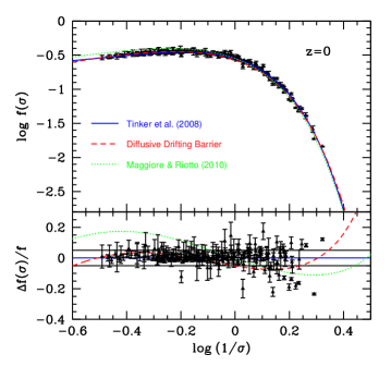
Figure 2: (Upper panel) Halo mass function at $z=0$ given by the Tinker et al. fitting formula for $\Delta=200$ (solid blue line), diffusing drifting barrier with ${\beta}=0.057$ and ${D}_{b}=0.294$ (red dashed line) and Maggiore & Riotto MaggioreRiotto2010b with $D_{B}=0.235$ (green dotted line). Data points are from Tinker2008 . (Lower panel) Relative difference with respect to the Tinker et al. fitting formula. The thin black solid lines indicates $5\%$ deviations.

In principle the values of $\beta$ and $D_{B}$ as well as their redshift and cosmology dependence can be predicted in a given halo collapse model by computing the average and variance of the probability distribution of the collapse density threshold. However, this requires a dedicated study which should also include environmental effects that have been shown to play an important role in determining the properties of the halo mass distribution Desjacques2008 . This goes beyond the scope of this Letter.

Here, we take a different approach. $\beta$ and $D_{B}$ are physical motivated model parameters which we can calibrate against N-body simulation data, and test whether the mass function derived above provides an acceptable description of the data. To this purpose we use the measurements of the halo mass function obtained by Tinker et al. Tinker2008 using SOD(200) on a set of WMAP-1 yr and WMAP-3 yr cosmological N-body simulations. For these cosmological models the spherical collapse predicts $\delta_{c}=1.673$ at $z=0$ (for a detailed calculation see Courtin2011 ). Using such a value, we run a likelihood Markov chain Monte Carlo analysis to confront the mass function previously computed against the data at $z=0$ in the prior parameter space $\log{\beta}=[-4,0]$ and $\log{D_{B}}=[-3,0]$. We find the best fit values to be ${\beta}=0.057$ and ${D}_{b}=0.294$. The data strongly constrain these parameters, with errors $\sigma_{\beta}=0.001$ and $\sigma_{D_{B}}=0.001$ respectively. In Fig. 2 (upper panel) we plot the corresponding mass function (red dash line) against the simulation data together with the four-parameter fitting formula by Tinker et al. Tinker2008 for $\Delta=200$ (solid blue line). For comparison we also plot the diffusive barrier case by Maggiore and Riotto MaggioreRiotto2010b which best fit the data with $D_{B}=0.235$ (green dotted line). In Fig. 2 (lower panel) we plot the relative differences with respect to the Tinker et al. formula. We may notice the remarkable agreement of the diffusive drifting barrier with the data. Deviations with respect to Tinker et al. (2008) are $\lesssim 5\%$ level over the range of masses probed by the simulations. This is quite impressive given the fact that our model depends only on two physically motivated parameters.

In the upcoming years a variety of astrophysical observations will directly probe $dn/dM$. The halo mass function we have derived here can provide the base for a through cosmological model comparison. In a companion paper we will describe in detail the derivation of these results, as well as extensive discussion on the redshift evolution of the mass function and halo bias.

- (1) D. N. Spergel et al., Astrophys. J. Suppl. Ser. 148, 175 (2003).
- (2) M. Tegmark et al., Phys. Rev. D. 69, 103501 (2004).
- (3) D. Clowe et al., Astrophys. J. 648, L109 (2006).
- (4) R. Massey et al., Nature (London) 445, 286 (2007).
- (5) W. H. Press and P. Schechter, Astrophys. J. 187, 425 (1974).
- (6) J. Tinker et al., Astrophys. J. 688, 709 (2008).
- (7) M. Crocce et al., Mont. Not. R. Astron. Soc. 403, 1353 (2010).
- (8) J. Courtin et al., Mont. Not. R. Astron. Soc. 410, 1911 (2011).
- (9) S. Batthacharya et al., Astrophys. J. 732, 122 (2011), arXiv:1005.2239.
- (10) J. R. Bond, S. Cole, G. Efstathiou and G. Kaiser, Astrophys. J. 379, 440 (1991).
- (11) A. R. Zentner, Int. J. Mod. Phys. D 16, 763 (2007).
- (12) W.J. Percival, Mont. Not. R. Astron. Soc. 327, 1313 (2001).
- (13) R. K. Sheth, Mont. Not. R. Astron. 300, 1057 (1998).
- (14) R. K. Sheth, H. J. Mo and G. Tormen, Mont. Not. R. Astron. 323, 1 (2001).
- (15) J. Shen, T. Abel, H. J. Mo and R. K. Sheth, Astrophys. J. 645, 783 (2006).
- (16) J. Zhang and L. Hui, Astrophys. J. 641, 641 (2006).
- (17) M. Maggiore and A. Riotto, Astrophys. J. 711, 907 (2010).
- (18) P.S. Corasaniti and I. Achitouv, PRD in press.
- (19) J. E. Gunn and J. R. Gott III, Astrophys. J. 176, 1 (1972).
- (20) A. G. Doroshkevich, Astrophyzika 3, 175 (1970).
- (21) D. J. Eisenstein and A. Loeb, Astrophys. J. 439, 520 (1995).
- (22) J. M. Bardeen, J. R. Bond, N. Kaiser and A. Szalay, Astrophys. J. 304, 15 (1986).
- (23) P. Monaco, Astrophys. J. 447, 23 (1995).
- (24) E. Audit, R. Teyssier and J.-M. Alimi, Astron. and Astrophys. 325, 439 (1997).
- (25) J. Lee and S. Shandarin, Astrophys. J. 500, 14 (1998).
- (26) V. Desjacques, Mont. Not. R. Astron. 388, 638 (2008).
- (27) B. Robertson, A. Kravtsov, J. Tinker and A. Zentner, Astrophys. J. 696, 636 (2009).
- (28) M. Maggiore and A. Riotto, Astrophys. J. 717, 515 (2010).
- (29) A. De Simone, M. Maggiore and A. Riotto, arXiv:1007.1903.
- (30) S. Redner, “A guide to first-passage processes”, Cambridge University Press, Cambridge, U.K. (2001).