Transport moments beyond the leading order

Abstract

For chaotic cavities with scattering leads attached, transport properties can be approximated in terms of the classical trajectories which enter and exit the system. With a semiclassical treatment involving fine correlations between such trajectories we develop a diagrammatic technique to calculate the moments of various transport quantities. Namely, we find the moments of the transmission and reflection eigenvalues for systems with and without time reversal symmetry. We also derive related quantities involving an energy dependence: the moments of the Wigner delay times and the density of states of chaotic Andreev billiards, where we find that the gap in the density persists when subleading corrections are included. Finally, we show how to adapt our techniques to non-linear statistics by calculating the correlation between transport moments.

In each setting, the answer for the $n$-th moment is obtained for arbitrary $n$ (in the form of a moment generating function) and for up to the three leading orders in terms of the inverse channel number. Our results suggest patterns which should hold for further corrections and by matching with the low order moments available from random matrix theory we derive likely higher order generating functions.

1 Introduction

Transport through a chaotic cavity is usually studied through a scattering description. For a chaotic cavity attached to two leads with $N_{1}$ and $N_{2}$ channels respectively, the scattering matrix is an $N\times N$ unitary matrix, where $N=N_{1}+N_{2}$. It can be separated into transmission and reflection subblocks

$$S(E)=\left(\begin{array}[]{cc}r_{1}&t^{\prime}\\ t&r_{2}\end{array}\right),$$ (1)

which encode the dynamics of the system and the relation between the incoming and outgoing wavefunctions in the leads. The unitarity of the scattering matrix $S^{\dagger}S=I=SS^{\dagger}$ leads to the following relations (among others)

$$r_{1}^{\dagger}r_{1}+t^{\dagger}t=I_{N_{1}},\qquad r_{2}r_{2}^{\dagger}+tt^{\dagger}=I_{N_{2}},$$ (2)

while the transport statistics themselves are related to the terms in (2) involving the scattering matrix (or its transmitting and reflecting subblocks) and their transpose conjugate. For example, the conductance is proportional to the trace $\Tr\left[t^{\dagger}t\right]$ (Landauer-Büttiker formula [1, 2, 3]), while other physical properties are expressible through higher moments like $\Tr\left[t^{\dagger}t\right]^{n}$.

There are two main approaches to studying the transport statistics in clean ballistic systems: a random matrix theory (RMT) approach, which argues that $S$ can be viewed as a random matrix from a suitable ensemble, and a semiclassical approach that approximates elements of the matrix $S$ by sums over open scattering trajectories through the cavity.

It was shown by Blümel and Smilansky [4, 5] that the scattering matrix of a chaotic cavity is well modelled by the Dyson’s circular ensemble of random matrices of suitable symmetry. Thus, transport properties of chaotic cavities are often treated by replacing the scattering matrix with a random one (see [6] for a review). The eigenvalues of the transmission matrix $t^{\dagger}t$ then follow a joint probability distribution, which depends on whether the system has time reversal symmetry or not, and from which transport moments and other quantities can be derived. Though the conductance and its variance were known for arbitrary channel number [7, 8], other quantities were limited to a diagrammatic expansions in inverse channel number, see [9]. However, the RMT treatment has recently experienced a resurgence due to the connection to the Selberg integral noticed in [10]. Following the semiclassical result for the shot noise [11], the authors of [10] used recursion relations derived from the Selberg integral to calculate the shot noise and then later all the various moments up to fourth order for arbitrary channel number [12].

Since then a range of transport quantities have been treated, for example the moments of the transmission eigenvalues for chaotic systems without time reversal symmetry (the unitary random matrix ensemble) [13, 14, 15, 16] and those with time reversal symmetry (the orthogonal random matrix ensemble) [15, 16]. For the unitary ensemble, the moments of the conductance itself were also obtained in [14] and, using a different approach, in [17] which was later extended to the moments of the shot noise [18]. Building again on the Selberg integral approach, the moments of the conductance and shot noise have been derived for both symmetry classes [19]. Interestingly these results, though all exact for arbitrary channel number, are given by different combinatorial sums, and the question of how they are related to each other is still open in many cases.

On the other hand, the semiclassical approach makes use of the following approximation for the scattering matrix elements [20, 21, 22]

$$S_{oi}(E)\approx\frac{1}{\sqrt{N\tau_{\mathrm{d}}}}\sum_{\gamma(i\to o)}A_{\gamma}(E)\rme^{\frac{\rmi}{\hbar}S_{\gamma}(E)},$$ (3)

which involves the open trajectories $\gamma$ which start in channel $i$ and end in channel $o$, with their action $S_{\gamma}$ and stability amplitude $A_{\gamma}$. The prefactor also involves $\tau_{\mathrm{d}}$ which is the average dwell time, or time the trajectory spends inside the cavity. For transport moments we consider quantities of the type

$$\left\langle\Tr\left[X^{\dagger}X\right]^{n}\right\rangle\sim\left\langle\frac{1}{{(N\tau_{\mathrm{d}})}^{n}}\prod_{j=1}^{n}\sum_{{i_{j},o_{j}}}\sum_{\substack{\gamma_{j}(i_{j}\to o_{j})\cr\gamma^{\prime}_{j}(i_{j+1}\to o_{j})}}A_{\gamma_{j}}A_{\gamma^{\prime}_{j}}^{*}\rme^{\frac{\rmi}{\hbar}(S_{\gamma_{j}}-S_{\gamma^{\prime}_{j}})}\right\rangle,$$ (4)

where the trace means we identify $i_{n+1}=i_{1}$ and where $X$ is either the transmitting or the reflecting subblock of the scattering matrix. The averaging is performed over a window of energies $E$.

The choice of the subblock $X$ affects the sums over the possible incoming and outgoing channels, but not the trajectory structure which involves $2n$ classical trajectories connecting channels. Of these, $n$ trajectories $\gamma_{j}$, $j=1,\ldots,n$, contribute with positive action while $n$ trajectories $\gamma^{\prime}_{j}$ contribute with negative action. In the semiclassical limit of $\hbar\to 0$ we require that these sums cancel on the scale of $\hbar$ so that the corresponding trajectories can contribute consistently when we apply the averaging in (4).

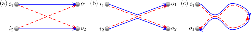
Figure 1: (a) The semiclassical trajectories for the second moment travel around a closed cycle. By collapsing the trajectories onto each other as in (b) we can create a small action difference and a trajectory quadruplet with a single encounter that contributes to the shot noise at leading order in inverse channel number. (c) For the conductance, a trajectory pair with a similar encounter provides the first subleading order correction for systems with time reversal symmetry.

The main idea of the semiclassical treatment is that, in order to achieve a small action difference, the trajectories $\{\gamma^{\prime}_{j}\}$, must follow the path of trajectories $\{\gamma_{j}\}$ most of the time, deviating only in small regions called encounters. This is best illustrated with an example. In figure 1(a) the schematic depiction of the trajectories is shown for the case $n=2$. We have 2 trajectories $\gamma$ depicted by solid lines, $\gamma_{1}:i_{1}\to o_{1}$ and $\gamma_{2}:i_{2}\to o_{2}$, and 2 trajectories $\gamma^{\prime}$ depicted by dashed lines, $\gamma^{\prime}_{1}:i_{2}\to o_{1}$ and $\gamma^{\prime}_{2}:i_{1}\to o_{2}$. Figure 1(b) shows one possible configuration for achieving a small action difference: trajectory $\gamma^{\prime}_{1}$ departs from the incoming channel $i_{2}$ following the path of trajectory $\gamma_{2}$. Then, when the trajectories $\gamma_{1}$ and $\gamma_{2}$ come close to each other in phase space (thus the term ‘encounter’), trajectory $\gamma^{\prime}_{1}$ switches from following $\gamma_{2}$ to following $\gamma_{1}$, before arriving at its destination channel $o_{1}$. The trajectory $\gamma^{\prime}_{2}$ does the opposite. The picture in figure 1(b) is referred to as a ‘diagram’; it describes the topological configuration of the trajectories in question, while leaving out metric details. The task of semiclassical evaluation can therefore be divided into two parts: evaluation of the contribution of a given diagram by integrating over all possible trajectories of given structure and enumeration of all possible diagrams.

Historically, the semiclassical treatment started with the mean conductance $\left\langle\Tr\left[t^{\dagger}t\right]\right\rangle$, involving a single trajectory and its partner. The leading order contribution comes from trajectory pairs that are identical — the so-called diagonal approximation which was evaluated in [23, 24]. The first non-diagonal pair was treated in [22] and involved a single encounter where one trajectory had a self-crossing while the partner avoided crossing as in figure 1(c). Such a pair can only exist when the system has time reversal symmetry and its contribution was shown to be one order higher in inverse channel number, $1/N$, than the diagonal terms. The expansion to all orders in inverse channel number was then performed in [25] for systems with and without time reversal symmetry by considering arbitrarily many encounters each involving arbitrarily many trajectory stretches.

Importantly, the work on the conductance [25] showed that the semiclassical contribution of a diagram can be decomposed into a product over the constituent parts of the diagram, greatly simplifying the resulting sums. In fact for the second moment, the shot noise, all such diagrams were generated in [11] and with them the full expansion in inverse channel number. This, along with the conductance variance and other transport correlation functions, as well as the semiclassical background was covered in detail in [26].

However, the method for diagram enumeration considered in [25, 11, 26] becomes unwieldy for higher moments, which encode finer transport statistics. To the leading order in $1/N$, the higher moments were derived in [27]. The semiclassical approach requires a large number of channels in each lead, $1\ll N_{1},N_{2}$, but to unambiguously separate the orders in inverse channel number one may additionally assume that both $N_{1}$ and $N_{2}$ are of the same order as $N$. For example, the result of [27] was in terms of the variable $\xi=N_{1}N_{2}/N^{2}$ which should then be constant and introduce no further channel number scaling. We therefore make the same assumption in this article when describing the different orders in $1/N$, though of course a different scaling, say keeping $N_{1}$ fixed so that $\xi\sim\mathrm{O}(1/N)$, may simply lead to a mixing of the different ‘orders’ without changing the individual results.

The diagrams contributing at the leading order to the $n$-th moment were shown in [27] to be trees. The tree expansions turned out to be very well suited to analysis of other interesting physical quantities, such as the statistics of the Wigner delay times [28], which are a measure of the time spent in the scattering region, and the density of states in Andreev billiards [29, 30]. If we imagine replacing the scattering leads by a superconductor we have a closed system called an Andreev billiard. Each time an electron inside the system hits the superconductor it is reflected as a hole retracing its path until it hits the superconductor and is retroreflected as an electron again. Wave interference between these paths leads to significant effects, most notably a complete suppression of the density of states for a range of energies around the Fermi energy. Similarly, strong effects on the conductance (of the order of the mean conductance) can also be seen if we attach additional superconducting leads to our original chaotic cavity (making a so-called Andreev dot) [31, 32]. The size of these effects make such systems especially interesting for a semiclassical treatment. But treating these effects effectively requires knowledge of all the higher moments, and gives us strong reason to go beyond low $n$.

One particular nicety of the semiclassical approach is that it can incorporate, in a natural way, the effect of the Ehrenfest time. This is the time scale that governs the transition from classical dynamics to wave interference, which dominates when the Ehrenfest time is small (on the scale of the typical dwell time). For larger Ehrenfest times, the competition between the different types of behaviour leads to quite striking features, like an additional gap both in the density of states of Andreev billiards and in the probability distribution of the Wigner delay times [30, 33]. Semiclassically we can explicitly track the effect of the Ehrenfest time all the way to the ‘classical’ limit, which can only be achieved using RMT by postulating the Ehrenfest time dependence of the scattering matrix.

Alongside the case of ballistic systems, the typical chaotic behaviour and transport statistics can also be induced by introducing disorder in the system. For weak disorder the transport properties coincide with those obtained from RMT, and one can also obtain the full counting statistics at leading order, as well as weak localisation corrections and universal conductance fluctuations, using circuit theory [34]. If the disorder averaging is treated using diagrammatic perturbation theory (see, for example, [35]) multiple scattering events can be summed, in the limit of weak disorder, as a ladder diagram known as a Diffuson. This corresponds to the parts of semiclassical diagrams where the trajectories are nearly identical, as on the left of the encounter in figure 1(c). The disordered systems’ counterpart of the loop on the right of the encounter in figure 1(c), traversed by trajectories in opposite directions, is called a Cooperon, while the encounter itself corresponds to a Hikami box [36]. Although transport properties like the weak localisation diagram related to figure 1(c) and conductance and energy level fluctuations [37] can be treated diagrammatically, usually powerful field-theoretic methods involving the nonlinear $\sigma$ model are used (see [38] for an introduction). These methods can treat both weak and stronger disorder non-perturbatively, and by using supersymmetry [39, 40] a large range of transport and spectral properties can be obtained, for open and closed systems correspondingly. More importantly, the applicability of RMT for weakly disordered systems can be justified and RMT shown to be the zero-dimensional variant of the $\sigma$ model [41, 42]. Alongside the supersymmetric $\sigma$ model, there is also the replica $\sigma$ model which is particularly useful for perturbative expansions. This leads to a diagrammatic expansion, with diagrams that can be reinterpreted as correlated semiclassical trajectories [43]. In fact this connection between semiclassical diagrams and disorder diagrams from the replica $\sigma$ model lay behind the semiclassical treatment of energy level correlations in closed systems [44, 45, 46] which in turn led to the semiclassical treatment of transport [22, 25, 26] discussed above.

To summarize, there are established semiclassical tools for the analysis of (4) for small $n$ to all orders of $1/N$ and for all $n$ but only to the leading order of $1/N$. It is the purpose of this article to start closing this gap. For all $n$ we derive the next two corrections for (4) and related quantities. We show that the contributing diagrams can be generated by grafting trees onto the ‘base diagrams’, which can be obtained by ‘cleaning’ the diagrams used in [25]. We therefore first review the leading order tree recursions in section 2 before treating transport moments beyond the leading order in section 3. We start by cleaning the diagram of figure 1(c) which gives the first subleading order orthogonal correction. Grafting trees onto the base diagram leads to a generating function, which we apply to calculate the moments of the transmission and reflection eigenvalues. Proceeding to the next order in $1/N$ we then treat the second subleading order diagrams for the unitary and the orthogonal case. For the moments of the reflection and transmission eigenvalues we find that our generating functions simplify and become rather straightforward.

The graphical recursions we use provide a new insight into the leading order terms which is particularly useful for energy dependent correlation functions. Such correlation functions are needed for a treatment of the density of states of Andreev billiards, which we consider in section 4 where we find that the hard gap, previously found at leading order in $1/N$, persists at least for the next two orders. Also derivable from energy dependent correlation functions are the moments of the Wigner delay times, treated in section 5, and we find that the corrections at each order in $1/N$ are also generated by relatively simple functions. Of course, the transport moments in (4) are only one type of transport quantity, and we finally look at non-linear statistics in section 6 and see how their treatment follows naturally from the previous semiclassical considerations.

We shall be comparing our semiclassical results with the prediction of RMT, where those predictions are available: previously (of the quantities treated here) only the moments of the transmission amplitudes for systems without time reversal symmetry have been given for an arbitrary number of channels [13, 14]. Explicit results for systems with time reversal symmetry have just been derived [15, 16] and we were pleased that [15] shared those results with us beforehand. The moments of the Wigner delay times for both symmetry classes have also been obtained [15].

Of the recent RMT results, it is those concerned with the asymptotic expansion as the number of channels increases, currently to leading order [47, 48, 49], that particularly connect with the work here. Semiclassically, without the equivalent of the Selberg integral, we are still restricted to an expansion in inverse powers of the channel number, but as we shall see the semiclassical treatment leads to explicit and surprisingly simple generating functions at each order in inverse channel number. This simplicity until now remained hidden in the combinatorial sums of the RMT results and may suggest ways of simplifying those results and of highlighting the underlying combinatorial structure.

2 Subtrees

The semiclassical treatment of the conductance beyond the diagonal contribution, starting [22] with the trajectory pair depicted in figure 1(c), required two main ingredients. The first was to estimate how often a trajectory would come close to itself and have a self-encounter. This is performed using the global ergodicity of the chaotic dynamics. The second was that, given such an encounter, we can use the local hyperbolicity of the motion to find the partner trajectory which reconnects the stretches of the original trajectory in a different way. Then one can determine the action difference between the two trajectories and hence their contribution in the semiclassical limit. When treating diagrams with more numerous and more complicated encounters, the authors of [25] showed that these two ingredients allowed them to express the total contribution as a product of integrals over the encounters and over the ‘links’, the trajectory stretches which connect the encounters together. Performing these integrals then led to simple rules for the contributions of the constituent parts of any diagram, and essentially reduced the problem down to the combinatorial one of finding all the possible diagrams. For the first two transport moments, this was done [26] by cutting open the periodic orbit pairs that contribute to spectral statistics [44, 45, 46].

For the higher moments, as shown in [27], the diagrams that contribute at leading order in inverse channel number are rooted plane trees. The reason is simple: according to the semiclassical evaluation rules of [26], every encounter contributes a factor of $-N$ while every link contributes a factor of $1/N$. The leading order is thus achieved by a diagram with the minimal possible difference between the number of links (edges) and encounters (internal vertices). It is a basic fact of graph theory that this difference is minimized by trees; each independent cycle in a graph adds one to this difference. Thus to go beyond the leading order one needs to consider diagrams with an increasing number of cycles. We will approach this task by describing the topology of the cycles using ‘base diagrams’ — graphs with no vertices of degree 1 or 2 — and then grafting subtrees onto the base diagrams.

Adding a subtree does not change the order of the contribution in inverse channel number $1/N$ but adds more incoming and outgoing channels thus changing the order of the moment $n$. Because we will be joining the trees to existing structures, unlike the treatment in [27, 28, 29, 30], here we do not root our trees in an incoming channel, but at an arbitrary point. These trees then correspond to the restricted trees in [27, 30] and will be referred to as ‘subtrees’. We also note that the generating function variables we use here have slightly different definitions than in [27, 28, 29, 30]. Our present choice is more appropriate for the subleading orders and the different transport quantities considered.

We now summarize the derivation of the subtree generating functions which were introduced in [27] and further developed in [28, 30]. A subtree consists of a root, several vertices of even degree (called ‘nodes’, they correspond to encounters between various trajectories) and $2n-1$ vertices of degree one (called ‘leaves’, they correspond to incoming or outgoing channels). The leaves are labelled $i$ or $o$ alternatingly as we go around the tree anti-clockwise. There are two types of subtrees: the $f$-subtrees have leaves labelled $o_{k}$, $i_{k+1}$, $o_{k+1}$, $i_{k+2}$ etc. The label $i_{k}$ would correspond to the root if we were to label it too. The $\hat{f}$-subtrees have leaf labels $i_{k+1}$, $o_{k+1}$, $i_{k+2}$, $o_{k+2}$ etc. The reference index $k$ depends on the location of the subtree on the diagram.

It is possible that an encounter happens immediately as several trajectories enter the cavity from the lead or exit the cavity into the lead. To keep account of these situations, we say that an $l$-encounter (node of degree $2l$) may ‘$i$-touch’ the lead if it is connected directly to $l$ incoming channels (leaves with label $i$) and ‘$o$-touch’ if connected to $l$ outgoing channels. When an encounter touches the lead, the edges connecting it to the lead get cut off and all the channels must coincide, although in the diagrams we keep short ‘stubs’ to avoid changing the degree of the encounter vertex.

We define the generating functions $f(\boldsymbol{x},\boldsymbol{z}_{i},\boldsymbol{z}_{o})$ and $\hat{f}=f(\boldsymbol{x},\boldsymbol{z}_{o},\boldsymbol{z}_{i})$ which are counting $f$- and $\hat{f}$-trees correspondingly. The meaning of the variables $\boldsymbol{x}=(x_{2},x_{3},\ldots)$, $\boldsymbol{z}_{i}=(z_{i,2},z_{i,3},\ldots)$ and $\boldsymbol{z}_{o}=(z_{o,2},z_{o,3},\ldots)$ is as follows:

• $x_{l}$ enumerate the $l$-encounters that do not touch the lead,

• $z_{i,l}$ enumerate the $l$-encounters that $i$-touch the lead,

• $z_{o,l}$ enumerate the $l$-encounters that $o$-touch the lead.

For example, the coefficient of $x_{3}x_{2}^{2}z_{i,2}$ gives the number of trees with one 3-encounter (a vertex of degree 6) and three 2-encounters (vertices of degree $4$), one of which $i$-touches the lead. An example of such a tree is given in figure 2(a). We note that if an encounter may touch the lead, the generating function includes (and sums) both possibilities: touching and non-touching. For example, the left-most vertex of the tree in figure 2(a) may $o$-touch the lead, but this possibility is counted separately.

In addition we will use several secondary parameters that will allow us to adapt the subtree generating functions to each of the four quantities considered in the paper. These parameters are:

• $y$ is the semiclassical contribution of an edge (link)

• $c_{i}$ and $c_{o}$ are the contributions of an incoming and an outgoing channel

• $\sigma$ is a special correction parameter for the situation when an $o$-touching node is directly connected to an $i$-channel ($\sigma=0$ everywhere apart from section 5).

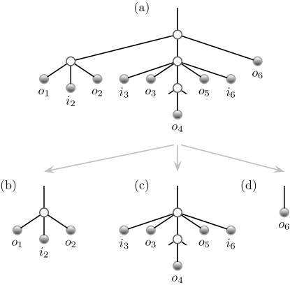
Figure 2: The subtree shown in (a) is cut at its top node (of degree 4) creating subtrees (b)-(d). Subtree (c) has the incoming and outgoing directions reversed. The lower vertex in (a), and hence (c), is $i$-touching the lead so that the channels $i_{4}$ and $i_{5}$ (not shown) coincide ($i_{4}=i_{5}$). This is represented by the short stubs, and the encounter now starts in the incoming lead.

We obtain a recursion for the functions $f$ and $\hat{f}$ by cutting the subtree at the top encounter node. If this node is of degree $2l$, this leads to $2l-1$ further subtrees as illustrated in figure 2. Assuming we started with an $f$-subtree, $l$ of the new subtrees also have type $f$, while the remaining $l-1$ are $\hat{f}$-subtrees. Thus an $f$-subtree with an $l$-encounter at the top contributes $yx_{l}f^{l}\hat{f}^{l-1}$ to the generating function $f$. Additionally, we consider the possibility for the top node of an $f$-subtree to $o$-touch. In this case its odd-numbered further subtrees are empty stubs and the even-numbered subtrees are still arbitrary, leading to the contribution $yz_{o,l}(\hat{f}+\sigma)^{l-1}$. Here we have included a correction term $\sigma$ which is used in section 5 to control the contribution of any $\hat{f}$-subtree that consists of one edge and directly connects an incoming and outgoing channel and is set to 0 in the rest of the paper.

We start our recursion relation at the value for an empty tree, which consists of a link (with the factor $y$) and an outgoing channel (providing a factor $c_{o}$),

$$f=yc_{o}+y\sum_{l=2}^{\infty}\left[x_{l}f^{l}{\hat{f}}^{l-1}+z_{o,l}(\hat{f}+\sigma)^{l-1}\right].$$ (5)

The recursion is similar for $\hat{f}$, with the roles of $i$- and $o$-variables switched,

$$\hat{f}=yc_{i}+y\sum_{l=2}^{\infty}\left[x_{l}{\hat{f}}^{l}{f}^{l-1}+z_{i,l}f^{l-1}\right].$$ (6)

2.1 Reflection

For the reflection into lead 1 we will consider the generating function

$$R(s)=\sum_{n=1}^{\infty}s^{n}\left\langle\Tr[r_{1}^{\dagger}r_{1}]^{n}\right\rangle,$$ (7)

where the power of $s$ counts the order of the moments. For the individual semiclassical diagrams we make use of the diagrammatic rules of [26], where each link contributes a factor of $1/N$ while each encounter provides the factor $-N$. Each channel is in lead 1, so can be chosen from the $N_{1}$ available and provides this factor. When an encounter starts (or ends) in the lead, all the incoming (or outgoing) channels must then coincide in the same channel, leading again to the factor $N_{1}$. Bearing in mind the meaning of the variables introduced above, we therefore have to make the following semiclassical substitutions:

$$y=\frac{1}{N},\quad x_{l}=-N,\quad z_{i,l}=z_{o,l}=r^{l}N_{1},\quad c_{i}=c_{o}=rN_{1},\quad\sigma=0,$$ (8)

where we have introduced $r$ whose power counts the total number of channels and which allows us to keep track of the total contributions to different moments. The $n$-th moment involves $2n$ channels so we have the relation $s=r^{2}$. Each channel factor $c$ then includes the factor $r$, while the formula for $z_{i,l}$ in (8) accounts for the fact that when an $l$-encounter enters the incoming channels we have $l$ channels coinciding but only a single channel factor.

If we define $\zeta_{1}=N_{1}/N$, the subtree recursions (5) and (6) both become

$$f=r\zeta_{1}-\sum_{l=2}^{\infty}f^{2l-1}+r\zeta_{1}\sum_{l=2}^{\infty}r^{l-1}f^{l-1}.$$ (9)

Performing the sums (where the terms $f$ and $r\zeta_{1}$ correspond to $l=1$ of the sums) this is

$$0=-\frac{f}{1-f^{2}}+\frac{r\zeta_{1}}{1-rf},$$ (10)

which can be written as the quadratic

$$r(1-\zeta_{1})f^{2}-f+r\zeta_{1}=0,\qquad f=\frac{1-\sqrt{1-4\xi r^{2}}}{2r(1-\zeta_{1})},$$ (11)

where $\xi=\zeta_{1}(1-\zeta_{1})$ and where we take the solution whose expansion agrees with the contributions of the semiclassical diagrams.

2.2 Transmission

For the transmission we treat the function

$$T(s)=\sum_{n=1}^{\infty}s^{n}\left\langle\Tr[t^{\dagger}t]^{n}\right\rangle,$$ (12)

and to distinguish it more clearly from the reflection we will call the corresponding subtree generating function $f=\phi$ here. For the transmission, the equations are a bit more complicated than for the reflection because $\phi\neq\hat{\phi}$ in general. For the substitution we need

$$y = \frac{1}{N},\quad x_{l}=-N,\quad z_{i,l}=r^{l}N_{1},\quad z_{o,l}=r^{l}N_{2},$$

$$c_{i} = rN_{1},\quad c_{o}=rN_{2},\quad\sigma=0,$$ (13)

where the only difference from (8) is that the outgoing channels are now in lead 2 and can be chosen from the $N_{2}$ available.

The contribution of the subtrees (5) once summed becomes

$$0=-\frac{\phi}{1-\phi\hat{\phi}}+\frac{r\zeta_{2}}{1-r\hat{\phi}},\qquad\mbox{or}\qquad\phi=r\zeta_{2}+r\zeta_{1}\phi\hat{\phi},$$ (14)

with $\zeta_{2}=N_{2}/N$ and using that $\zeta_{1}+\zeta_{2}=1$. Likewise (6) becomes

$$0=-\frac{\hat{\phi}}{1-f\hat{\phi}}+\frac{r\zeta_{1}}{1-r\phi},\qquad\mbox{or}\qquad\hat{\phi}=r\zeta_{1}+r\zeta_{2}\phi\hat{\phi},$$ (15)

where, as before $\xi=\zeta_{1}(1-\zeta_{1})=\zeta_{1}\zeta_{2}$. With $h=\phi\hat{\phi}$ we have

$$r^{2}\xi h^{2}+[r^{2}(1-2\xi)-1]h+r^{2}\xi=0,$$ (16)

from which we can find the equations

$$\phi^{2}-\left(\frac{1-r^{2}}{r\zeta_{2}}+2r\right)\phi+1=0,\qquad\hat{\phi}^{2}-\left(\frac{1-r^{2}}{r\zeta_{1}}+2r\right)\hat{\phi}+1=0.$$ (17)

3 Transport moments

By a simple counting argument, the order of a diagram in terms of inverse channel number is the number of edges minus the number of vertices (both leaves and nodes). Thus a diagram contributes at the order $(1/N)^{\beta-1}$, where $\beta$ is the number of the independent cycles in the diagram (also known as the cyclomatic number or the first Betti number, hence the notation). The leading contribution thus comes from tree diagrams which have $\beta=0$ and the next contribution comes from diagrams with one cycle.

3.1 First orthogonal correction

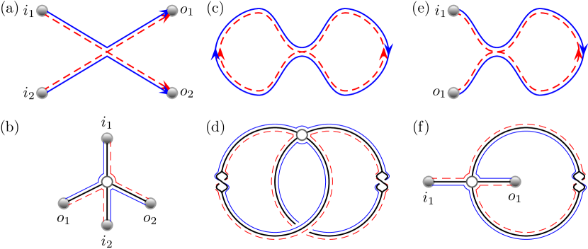
Figure 3: The correlated trajectory quadruplet in (a) which contributes to the second moment at leading order in inverse channel number can be redrawn as the ribbon tree in (b) by ‘untwisting’ the encounter. The four trajectories themselves can be read off from the boundary walk shown. At subleading order in inverse channel number, we start with the correlated periodic orbit pair in (c) which can be represented as the graph in (d) with corresponding boundary walks. Cutting the periodic orbit along the left link (which is traversed in the same direction by the orbit and its partner) creates the correlated trajectory pair in (e) which contributes to the first moment. Changing this diagram into a graph we arrive at the structure in (f) which is a Möbius strip with an empty subtree inside and outside the loop. The intertwined S’s in diagrams (d) and (f) represent twists in the corresponding ribbon links.

A diagram with one cycle can be thought of as a loop with trees grafted on it. But there is a twist. The reconstruction of the trajectories’ structure from a tree, see [27], was done by means of the boundary walk. It helps to visualise the edges of the tree as strips, a model that is called a fat or ribbon graph in combinatorics. This fixes the circular order of edges around each vertex and, going along the boundary, prescribes a unique way to continue the walk around a vertex (see [50] for an accessible introduction). The trajectories $\gamma_{j}$ of equation (4) are then read as the portions of the walk going from $i_{j}$ to $o_{j}$. The trajectories $\gamma_{j}^{\prime}$, on the other hand, appear in reverse as portions of the walk going from $o_{j}$ to $i_{j+1}$. For example, the diagram in figure 3(a) which contributes at leading order in $1/N$ can be redrawn as the tree in figure 3(b) with the corresponding boundary walk shown.

The trace in (4) means that the boundary walk is closed and the equality of total actions implies that each edge of the diagram is traversed twice (once by $\gamma$ and once by $\gamma^{\prime}$). This means that a valid diagram must have one face. In particular, there must be a way for the walk to cross from inside to outside of the cycle of the first correction diagram. The diagram thus has the topology of a Möbius strip with (ribbon) trees grafted on the edges. We will refer to the diagram without any trees (Möbius strip in this case) as the base diagram or structure.

It is also beneficial to consult the full expansion in powers of the inverse channel number of the first two moments of the transmission eigenvalues [22, 25, 11, 26] and to draw the corresponding diagrams as ribbon graphs. The procedure of going from the closed periodic orbits to scattering trajectories and then to a graph is illustrated in figure 3 for the first subleading order correction. Removing the remaining subtrees from figure 3(f) leads to the base structure in figure 4(a) to which we can append subtrees to create valid diagrams like figure 4(b) whose boundary walk is depicted in figure 4(c). As the base structure involves a loop which is traversed in opposite directions by the trajectory and its partner, all the diagrams created in this way can only exist in systems with time reversal symmetry (corresponding to the orthogonal RMT ensemble).

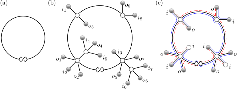
Figure 4: To obtain the base structure in (a) we can simply remove the empty subtrees of figure 3(f). Appending subtrees to (a) we can then create all the possible graphs, but for the graph to remain a Möbius strip we need an odd number of odd nodes, as for example in the graph in (b). We draw the boundary walk in (c) where we truncated the subtrees at their first node as they always have an odd number of leaves thereafter. The top left and bottom right nodes along the Möbius strip in (b) or (c) may also enter the lead for reflection quantities.

Along the loop we can add subtrees at any point and to make a valid $l$-encounter we must add $2l-2$ subtrees (the remaining two stretches in the encounter belong to the loop itself). If the node has an odd number of trees both inside and outside the loop, we refer to it as an odd node. It is easy to convince oneself that in order to have each stretch of the loop traversed once by a $\gamma$-trajectory and once by a $\gamma^{\prime}$-trajectory there must be an odd number of odd nodes around the loop.

We start by evaluating the contribution of a node along the loop. For the node we include all possible sizes $l$ of the resulting encounter. Adding the $2l-2$ subtrees (of which $l-1$ start with an incoming direction and $l-1$ with an outgoing direction) there are $2l-1$ ways of splitting them into groups inside or outside of the encounter. With the $l-1$ ways which result in an odd node we include the factor $p$ whose power will later count the total number of odd nodes around the loop. This leads to

$$A(p)=\sum_{l=2}^{\infty}x_{l}(f\hat{f})^{l-1}[p(l-1)+l].$$ (18)

The number of incoming and outgoing channels connected to the same node is equal [see an example in figure 4(b)]. An $l$-encounter can touch the lead only if every other edge connected to it is empty (connected directly to a leaf). Since for nodes on the loop we need to include the edges that belong to the loop itself and which cannot be empty, we conclude that only odd nodes can possibly touch the lead. Since in this case we need $l$ empty edges and we have $l-1$ edges of each type, touching the lead is possible only if the incoming and outgoing channels are in the same lead, as they are when we consider a reflection quantity.

With $2k-1$ trees on the inside of which $k$ must be empty (and the remaining $k-1$ arbitrary) and the remaining $2l-2k-1$ on the outside (with $l-k$ empty and $l-k-1$ arbitrary) and with $\boldsymbol{z}_{i}=\boldsymbol{z}_{o}=\boldsymbol{z}$ for reflection quantities we add the following to the node contribution

$$B(p)=\sum_{l=2}^{\infty}z_{l}\sum_{k=1}^{l-1}pf^{k-1}(\hat{f}+\sigma)^{l-k-1}.$$ (19)

We then allow any number of nodes along the loop, though each time we add a new node it creates a new edge of the loop. Because of the rotational symmetry, we divide by the number of nodes. In addition, there is a symmetry between the inside and the outside of the loop, leading to a factor of $1/2$. The total contribution thus becomes

$$\tilde{K}_{1}=\frac{1}{2}\sum_{k=1}^{\infty}\frac{[y(A+B)]^{k}}{k}=-\frac{1}{2}\ln[1-y(A+B)].$$ (20)

Finally, to ensure that we have an odd number of odd nodes along the loop, we set

$$K_{1}=\frac{\tilde{K}_{1}(p=1)-\tilde{K}_{1}(p=-1)}{2}.$$ (21)

This function then generates all the diagrams with $2n$ channels. We can now choose any of the leaves to be labelled $i_{1}$, which fixes the numbering of all other leaves: they are numbered in order along the boundary walk. The freedom of choosing one of the leaves gives a factor of $2n$. To get this factor we differentiate the result with respect to $r$ and multiply by $r$ so that the power of $r$ still counts the total number of channels. Thus we obtain the generating function

$$F=r\frac{\rmd K}{\rmd r}.$$ (22)

For the transmission, using the semiclassical values of the variables in (13), we find that the node contribution in (18) becomes

$$A(p)=\frac{Nh(h-p-2)}{(1-h)^{2}}.$$ (23)

As we do not allow the nodes to enter the leads (as the incoming and outgoing channels are now in different leads) we also have $B=0$. Note that the node contribution is given solely in terms of $h=\phi\hat{\phi}$ and the full contribution evaluates to

$$K_{1}=\frac{1}{4}\ln\left(\frac{1-h}{1+h}\right).$$ (24)

Putting in the correct explicit solution for $h$ from (16) and transforming according to (22), we find the following generating function for the orthogonal correction to the moments of the transmission eigenvalues

$$T_{1}(s)=-\frac{\xi s}{(1-s)(1-s+4\xi s)},$$ (25)

where we set $s=r^{2}$ to generate the moments as the $n$-th moment involves $2n$ channels. This order correction was previously treated using a RMT diagrammatic expansion [9], and can be derived by performing an asymptotic expansion in inverse channel number of the RMT result for arbitrary channel number of [15].

For the reflection we have $\hat{f}=f$ and the node contributions in (18) and (19) are

$$A(p)=\frac{Nf^{2}(f^{2}-p-2)}{(1-f^{2})^{2}},\qquad B(p)=\frac{pN\zeta_{1}r^{2}}{(1-rf)^{2}}.$$ (26)

Using relation (10) we can rewrite $B(p)$ as

$$B(p)=\frac{pN}{\zeta_{1}}\frac{f^{2}}{(1-f^{2})^{2}},$$ (27)

so that for the generating function we find

$$K_{1}=\frac{1}{4}\ln\left(\frac{\zeta_{1}+\zeta_{2}f^{2}}{\zeta_{1}-\zeta_{2}f^{2}}\right)=\frac{1}{4}\ln\left(\frac{f}{2r\zeta_{1}-f}\right),$$ (28)

where for the last term we simplified the numerator and denominator inside the logarithm by only keeping the remainder after polynomial division with respect to the quadratic for $f$ in (11). Putting in the explicit solution from (11) and following (22) we obtain the rather simple generating function for the orthogonal correction to the moments of the reflection eigenvalues

$$R_{1}(s)=\frac{\xi s}{(1-4\xi s)}.$$ (29)

Note that this result only depends on $\xi=\zeta_{1}(1-\zeta_{1})=\zeta_{1}\zeta_{2}$, which is not so obvious from (28) and (11). However, the relations in (2) and the fact that the trace of the identity matrix, being the respective number of channels, is only leading order in inverse channel number means that the dependence only on $\xi$ of the subleading transmission moments (25) must be mirrored in the reflection moments. For the reflection into lead 2 we simply swap $\zeta_{1}$ and $\zeta_{2}$, which clearly does not affect this order correction.

3.2 Unitary correction

We can continue using the ideas above to treat higher order corrections. In particular, for systems without time reversal symmetry the first correction occurs at the second subleading order in inverse channel number. The semiclassical diagrams for the conductance are given, for example, in [26] and can be represented as the graph diagrams shown in figures 5(a) and (b). We note that this representation is not unique and is chosen for simplicity. It is also important to observe that, despite the twists, the corresponding ribbon graphs are orientable, i.e. have two surfaces (unlike the Möbius strip). It can be shown this is true in general: diagrams contributing to the unitary case are orientable. Further, the diagrams contributing at this order have genus 1, i.e. embeddable on a torus (but not a sphere). This, too, can be shown to continue: the contribution to the order $1/N^{(2g-1)}$ comes from diagrams of genus $g$.

From the diagrams in figures 5(a) and (b) we can form the base structures by removing the channels and their links, see figures 5(c) and (d). A similar restriction to the one above still holds when appending subtrees to ensure that the resulting diagrams are permissible. Namely, the total number of odd nodes and twists along every closed cycle in the diagram has to be even. We note that the definition of an odd node depends on the cycle: the left node of figure 5(a) is odd with respect to the cycles formed from the top and bottom arcs and is even relative to the cycle formed from the top arc and the middle edge. We remark that this rule was enforced for the Möbius diagram as well.

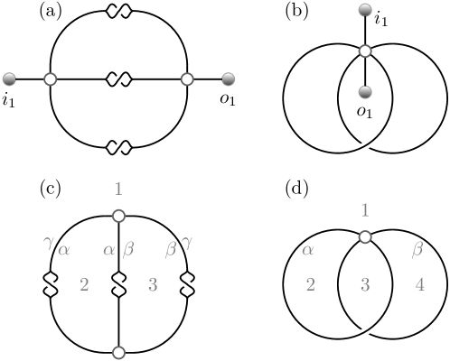
Figure 5: The first subleading order semiclassical diagrams for systems without time reversal symmetry. We start with the trajectory pairs which contribute to the conductance in (a) and (b). Removing the channels and their links we obtain the base structures (c) and (d) for this case.

Finally, we need to discuss the symmetries of each base diagram. The generators of the symmetry group of base diagram 5c are the shift of the edge numbering and the reflection, giving a group of size 6. The generators for base diagram 5d are inside-outside mappings of the two edges, giving a group of size 4.

When we append subtrees along each edge of a diagram, whether we append $f$ or $\hat{f}$-type subtrees depends in a complicated way on the types of subtrees appended along the other edges. Therefore we restrict ourselves to the simpler situation where $f=\hat{f}$ and only treat reflection quantities (with $\sigma=0$). Along the links connecting the nodes in the base diagrams we can append subtrees as before, but because the rotational symmetry is now broken we no longer divide by the number of nodes. The edge contributions can therefore be written as

$$E(p)=y\sum_{k=0}^{\infty}[y(A+B)]^{k}=\frac{y}{1-y(A+B)},$$ (30)

where $A(p)$ and $B(p)$ are as in (18) and (19) but with the simplification $f=\hat{f}$ and $\sigma=0$.

We also need to append subtrees to the nodes of the base structures and, finally, ensure that we have the correct number of objects (odd nodes and twists) around each closed cycle. To proceed, we number each of the regions around the nodes and label the closed cycles with greek letters as in figures 5(c) and (d). We start with figure 5(c) and use powers of $p_{\alpha}$, $p_{\beta}$ and $p_{\gamma}$ to count the number of objects along the respective cycles. At the top node we can add subtrees in any region we like as long as we add an odd number in total to ensure that the top node becomes a valid $l$-encounter. An $l$-encounter involves $2l$ stretches and we have 3 stretches already from the base structure. If we place $k_{i}$ subtrees in each region $i$ and use the power of $q$ to count the total number of subtrees added, we can write the contribution of the top node as

$$\tilde{V}_{3\mathrm{c}}(q)=\sum_{k_{1},k_{2},k_{3}=0}^{\infty}x_{l}(qf)^{(k_{1}+k_{2}+k_{3})}p_{\alpha}^{k_{2}}p_{\beta}^{k_{3}}p_{\gamma}^{k_{1}},$$ (31)

with $l=(k_{1}+k_{2}+k_{3}+3)/2$ and where the number 3 in the subscript refers to the fact that the node in the base diagram starts with 3 stretches while the ‘c’ refers to its label in figure 5. Further, when we have an odd number of trees in each region, and when the odd numbered trees in each region are empty, then the top node can also enter the lead (since we are considering reflection quantities). If we define $k_{i}=2\tilde{k}_{i}+1$ then we have $\tilde{k}_{i}+1$ empty subtrees and $\tilde{k}_{i}$ arbitrary subtrees in each region. In total we would then add the contribution

$$\tilde{V}^{\prime}_{3\mathrm{c}}(q)=qp_{\alpha}p_{\beta}p_{\gamma}\sum_{\tilde{k}_{1},\tilde{k}_{2},\tilde{k}_{3}=0}^{\infty}z_{l}f^{(\tilde{k}_{1}+\tilde{k}_{2}+\tilde{k}_{3})},$$ (32)

where $l=(\tilde{k}_{1}+\tilde{k}_{2}+\tilde{k}_{3}+3)$ and we simplified the powers of $q$ and $p$ as in the end we are only interested in whether they are odd or even and they are all odd here. Finally to ensure that the total number of trees added is odd, we substitute

$$V_{3\mathrm{c}}=\frac{\tilde{V}_{3\mathrm{c}}(q=1)-\tilde{V}_{3c}(q=-1)}{2}+\tilde{V}^{\prime}_{3\mathrm{c}}(q=1).$$ (33)

The complete diagram in figure 5(c) is made up of two such nodes as well as three links. Each of the links lies on two cycles so we can write the full contribution as

$$\tilde{K}^{\mathrm{U}}_{2\mathrm{c}}=\frac{1}{6}E(p_{\alpha}p_{\beta})E(p_{\beta}p_{\gamma})E(p_{\gamma}p_{\alpha})(V_{3\mathrm{c}})^{2}$$ (34)

where we divide by 6 to account for the symmetry of the base structure. Here the number in the subscript now refers to the order of the contribution while the ‘U’ in the superscript refers to the fact that these diagrams correspond to the unitary ensemble. Then to ensure that the number of objects along each cycle is even we simply average

$$K^{\mathrm{U}}_{2\mathrm{c}}=\frac{\tilde{K}^{\mathrm{U}}_{2\mathrm{c}}(p=1)+\tilde{K}^{\mathrm{U}}_{2\mathrm{c}}(p=-1)}{2},$$ (35)

for $p_{\alpha}$, $p_{\beta}$ and $p_{\gamma}$ in turn.

For the base structure in figure 5(d) we now have a single node and four regions. Region 3 lies inside both cycles and each cycle starts with a single object inside (and likewise outside) which are the stretches of the other cycle leaving or entering the node. Treating the node as above, we obtain the contributions

$$\tilde{V}_{4\mathrm{d}}(q)=\sum_{k_{1},k_{2},k_{3},k_{4}=0}^{\infty}x_{l}(qf)^{(k_{1}+k_{2}+k_{3}+k_{4})}p_{\alpha}^{k_{2}}(p_{\alpha}p_{\beta})^{k_{3}}p_{\beta}^{k_{4}},$$ (36)

with $l=(k_{1}+k_{2}+k_{3}+k_{4}+4)/2$ and

$$\tilde{V}^{\prime}_{4\mathrm{d}}(q)=\sum_{\tilde{k}_{1},\tilde{k}_{2},\tilde{k}_{3},\tilde{k}_{4}=0}^{\infty}z_{l}f^{(\tilde{k}_{1}+\tilde{k}_{2}+\tilde{k}_{3}+\tilde{k}_{4})},$$ (37)

where $l=\tilde{k}_{1}+\tilde{k}_{2}+\tilde{k}_{3}+\tilde{k}_{4}+4$ and with an odd number of trees in each region in this second case we are guaranteed to add an even number to each cycle and an even number overall. With four edges touching the node in the base structure we need to add an even number of subtrees in total to the node to make a valid $l$-encounter so the node contribution reduces to

$$V_{4\mathrm{d}}=\frac{\tilde{V}_{4\mathrm{d}}(q=1)+\tilde{V}_{4\mathrm{d}}(q=-1)}{2}+\tilde{V}^{\prime}_{4\mathrm{d}}(q=1).$$ (38)

Including the two edges we have a total contribution of

$$\tilde{K}^{\mathrm{U}}_{2\mathrm{d}}=\frac{1}{4}p_{\alpha}p_{\beta}E(p_{\alpha})E(p_{\beta})V_{4\mathrm{d}},$$ (39)

where we divide by 4 to account for the symmetry of the diagram and the $p_{\alpha}p_{\beta}$ accounts for the fact that the cycles each start with a single object (the original node, which is odd for both cycles). We likewise take the average

$$K^{\mathrm{U}}_{2\mathrm{d}}=\frac{\tilde{K}^{\mathrm{U}}_{2\mathrm{d}}(p=1)+\tilde{K}^{\mathrm{U}}_{2\mathrm{d}}(p=-1)}{2},$$ (40)

for $p_{\alpha}$ and $p_{\beta}$ in turn.

When we put in the semiclassical substitutions from (8) the formulae above can be summed and simplified. After applying the operator $r\frac{\rmd}{\rmd r}$ we find that first correction for the reflection for the unitary case (adding the two base cases) has the generating function

$$NR^{\mathrm{U}}_{2}(s)=\frac{\xi^{2}s^{2}(s-1)}{(1-4\xi s)^{\frac{5}{2}}},$$ (41)

By restricting ourselves above to the situation where $f=\hat{f}$ we are not able to obtain the transmission directly, but we can instead find the likely transmission generating function using (2) that $t^{\dagger}t+r_{1}^{\dagger}r_{1}=I$

$$NT^{\mathrm{U}}_{2}(s)=-\frac{\xi^{2}s^{2}}{(1-s)^{\frac{3}{2}}(1-s+4\xi s)^{\frac{5}{2}}}.$$ (42)

The fact that we get such simple functions is a little surprising especially as the result from each base case is notably more complex. In fact this pattern can be seen to continue if we expand the RMT result as in A. The generating function in (42) can also be obtained [15] from their RMT result.

3.3 Second orthogonal correction

When the system has time reversal symmetry, the edges and encounters can again be traversed in different directions by the trajectory set and their partners. For the conductance there are 7 further semiclassical diagrams at this order as depicted, for example in [26]. When we remove the starting and end links to arrive at the base structures, we find that they reduce to the 4 base cases depicted in figure 6.

We note that the additional diagrams are non-orientable when viewed as ribbon graphs. Their groups of symmetry contain two elements each: reflection for diagrams 6(a)–(c) and inside-out flipping of both edges simultaneously for diagram 6(d).

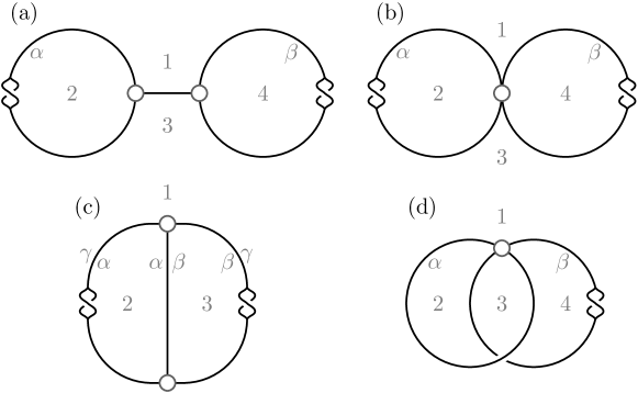
Figure 6: The additional 4 base structures that exist for systems with time reversal symmetry at the second subleading order in inverse channel number.

Figures 6(c) and (d) are almost the same as figures 5(c) and (d), so we start with evaluating the contribution of figure 6(a). Although region 1 and 3 are spatially connected they differ as to where we append subtrees at the nodes. Starting with the node on the left we therefore get the contributions

$$\tilde{V}_{3\mathrm{a}}(q)=\sum_{k_{1},k_{2},k_{3}=0}^{\infty}x_{l}(qf)^{(k_{1}+k_{2}+k_{3})}p_{\alpha}^{k_{2}},$$ (43)

with $l=(k_{1}+k_{2}+k_{3}+3)/2$ and

$$\tilde{V}^{\prime}_{3\mathrm{a}}(q)=qp_{\alpha}\sum_{\tilde{k}_{1},\tilde{k}_{2},\tilde{k}_{3}=0}^{\infty}z_{l}f^{(\tilde{k}_{1}+\tilde{k}_{2}+\tilde{k}_{3})}.$$ (44)

Again to ensure that an odd number of trees are appended, we substitute

$$V_{3\mathrm{a}}=\frac{\tilde{V}_{3\mathrm{a}}(q=1)-\tilde{V}_{3a}(q=-1)}{2}+\tilde{V}^{\prime}_{3\mathrm{a}}(q=1).$$ (45)

For the node on the right we obtain the contribution $\hat{V}_{3\mathrm{a}}$ which is the same as $V_{3\mathrm{a}}$ but with $p_{\alpha}$ swapped with $p_{\beta}$ (and also $k_{2}$ with $k_{4}$).

Along with the two nodes in figure 6(a) we have three links, two of which form cycles which already contain a single object (a twist). The total contribution is then

$$\tilde{K}^{\mathrm{O}}_{2\mathrm{a}}=\frac{1}{2}p_{\alpha}p_{\beta}E(p_{\alpha})E(1)E(p_{\beta})V_{3\mathrm{a}}\hat{V}_{3\mathrm{a}},$$ (46)

and to have an even number of objects along both cycles we average

$$K^{\mathrm{O}}_{2\mathrm{a}}=\frac{\tilde{K}^{\mathrm{O}}_{2\mathrm{a}}(p=1)+\tilde{K}^{\mathrm{O}}_{2\mathrm{a}}(p=-1)}{2},$$ (47)

for $p_{\alpha}$ and $p_{\beta}$ in turn.

The node in the base structure in figure 6(b) provides the following contributions

$$\tilde{V}_{4\mathrm{b}}(q)=\sum_{k_{1},k_{2},k_{3},k_{4}=0}^{\infty}x_{l}(qf)^{(k_{1}+k_{2}+k_{3}+k_{4})}p_{\alpha}^{k_{2}}p_{\beta}^{k_{4}},$$ (48)

with $l=(k_{1}+k_{2}+k_{3}+k_{4}+4)/2$ and

$$\tilde{V}^{\prime}_{4\mathrm{b}}(q)=p_{\alpha}p_{\beta}\sum_{\tilde{k}_{1},\tilde{k}_{2},\tilde{k}_{3},\tilde{k}_{4}=0}^{\infty}z_{l}f^{(\tilde{k}_{1}+\tilde{k}_{2}+\tilde{k}_{3}+\tilde{k}_{4})}.$$ (49)

The total number of trees added must be even, leading to

$$V_{4\mathrm{b}}=\frac{\tilde{V}_{4\mathrm{b}}(q=1)+\tilde{V}_{4\mathrm{b}}(q=-1)}{2}+\tilde{V}^{\prime}_{4\mathrm{b}}(q=1),$$ (50)

while with the two cycles (which each start with a single object) we have a total contribution of

$$\tilde{K}^{\mathrm{O}}_{2\mathrm{b}}=\frac{1}{2}p_{\alpha}p_{\beta}E(p_{\alpha})E(p_{\beta})V_{4\mathrm{b}}.$$ (51)

As before we take the average

$$K^{\mathrm{O}}_{2\mathrm{b}}=\frac{\tilde{K}^{\mathrm{O}}_{2\mathrm{b}}(p=1)+\tilde{K}^{\mathrm{O}}_{2\mathrm{b}}(p=-1)}{2},$$ (52)

for $p_{\alpha}$ and $p_{\beta}$ in turn.

The difference of the structure in figure 6(c) from that in figure 5(c) is that now cycles $\alpha$ and $\beta$ start with an odd number of objects. The contribution is then

$$\tilde{K}^{\mathrm{O}}_{2\mathrm{c}}=\frac{1}{2}p_{\alpha}p_{\beta}E(p_{\alpha}p_{\beta})E(p_{\beta}p_{\gamma})E(p_{\gamma}p_{\alpha})(V_{3\mathrm{c}})^{2}$$ (53)

before averaging over the $p$’s in turn. Only the $\alpha$ cycle in the structure in figure 6(d) now starts with an odd number of objects so its contribution is

$$\tilde{K}^{\mathrm{O}}_{2\mathrm{d}}=\frac{1}{2}p_{\alpha}E(p_{\alpha})E(p_{\beta})V_{4\mathrm{d}},$$ (54)

and then we average over $p_{\alpha}$ and $p_{\beta}$ in turn.

Summing over the four new base cases (as well as the two that also exist without time reversal symmetry) we obtain the second subleading correction for the orthogonal case

$$NR^{\mathrm{O}}_{2}(s)=-\frac{\xi s\left[\xi s(3+s)+1-2s\right]}{(1-4\xi s)^{\frac{5}{2}}}.$$ (55)

From this we can again find the likely generating function for the transmission

$$NT^{\mathrm{O}}_{2}(s)=\frac{\xi s\left[\xi s(4s-3)+1-s^{2}\right]}{(1-s)^{\frac{3}{2}}(1-s+4\xi s)^{\frac{5}{2}}}.$$ (56)

The moments generated by (56) can be proven [15] to to agree with the moments obtained from an asymptotic expansion of their RMT result. Semiclassically, time reversal symmetry allows more possible diagrams, so the results here are somewhat more complicated than the results (41) and (42) for systems without time reversal symmetry, but the RMT result [15] for the orthogonal case is notably more complex than for the unitary case. The results here are therefore useful in simplifying asymptotic expansions of RMT moments.

3.4 Leading order revisited

To obtain the leading order contributions [27], the start of the tree was fixed in the first incoming channel $i_{1}$ which allowed the top node to possibly $i$-touch. For example we simply place an incoming channel on top of the tree in figure 2(a). If the odd numbered subtrees after the top node were empty then the top node could $i$-touch the lead, leading to the generating function [28]

$$F_{0}=c_{i}f+\sum_{l=2}^{\infty}z_{i,l}f^{l}+c_{o}\sigma+\sigma\sum_{l=2}^{\infty}z_{o,l}(\hat{f}+\sigma)^{l-1}.$$ (57)

Here the terms involving $\sigma$ derive from the fact that the section of the tree above the top node is actually an empty $\hat{f}$ tree.

However, using the ideas we developed for the subleading corrections we can imagine a way of generating the leading order trees without fixing any of the channels as a root. As we shall see this is particularly beneficial for calculating energy dependent correlation functions as in sections 4 and 5. To start, we view a single point as the base structure for the leading order diagrams. We therefore obtain the leading order diagrams by joining subtrees to this point. To create a valid encounter we need to add $2l$ subtrees (with $l\geq 2$), $l$ of which are $f$-type subtrees starting from an incoming direction and the other $l$ are $\hat{f}$-type subtrees. If all of the subtrees of a particular type are empty then the node created can touch the lead. We obtain the generating function

$$\tilde{K}_{0}=\sum_{l=2}^{\infty}\frac{x_{l}(f\hat{f})^{l}}{2l}+\sum_{l=2}^{\infty}\frac{z_{i,l}f^{l}}{2l}+\sum_{l=2}^{\infty}\frac{z_{o,l}(\hat{f}+\sigma)^{l}}{2l},$$ (58)

where we divide by $l$ because of the rotational symmetry and by a further factor of 2 because of the additional possibility of swapping the incoming and outgoing channels. The last two terms in (58) represent moving the $l$-encounter (formed by appending the subtrees to the starting point) into the incoming and outgoing channels. Importantly we overcount the trees by the factor $V$ of their total number of encounters because, for a given resulting tree, any of the nodes could have been used as the base structure.

On the other hand we can also construct trees by joining two subtrees together, one $f$-type and one $\hat{f}$-type. After joining, the new vertex of degree two gets absorbed into the edge. A tree has exactly $V-1$ internal edges, therefore there are $V-1$ ways to obtain a given tree from joining two subtrees. The joining operation gives the contribution

$$\tilde{K}^{\prime}_{0}=\frac{1}{2y}(f-yc_{o})(\hat{f}-yc_{i})-\frac{1}{2}c_{o}(yc_{i}+\sigma),$$ (59)

where we divide by 2 because of the symmetry of swapping the incoming and outgoing channels. In the first term in (59) we subtract the empty tree from both $f$ quantities to ensure that they both include at least one node so that the edge formed is an internal one. The last term in (59) is then to ensure that the diagram made of a single diagonal link with no encounters ($V=0$) is included with the correct factor of $-1/2$. Taking the difference between (58) and (59) then means that we count each tree exactly once. Fittingly, for all the physical quantities we consider in this article (59) equals minus the $l=1$ term in the sums in (58). This is natural because by joining two subtrees we essentially create a 1-encounter. We simplify the difference to

$$K_{0}=\tilde{K}_{0}-\tilde{K}^{\prime}_{0}=\sum_{l=1}^{\infty}\frac{x_{l}(f\hat{f})^{l}}{2l}+\sum_{l=1}^{\infty}\frac{z_{i,l}f^{l}}{2l}+\sum_{l=1}^{\infty}\frac{z_{o,l}(\hat{f}+\sigma)^{l}}{2l}.$$ (60)

Now that no root is fixed we can make any channel to be the first incoming channel and this generating function indeed misses a factor $2n$ compared to the generating function $F$. This turns out to be very useful for the density of states of Andreev billiards in section 4 and to recover $F$ we can use relation (22).

The generating function (57) for the reflection into lead 1 becomes

$$F_{0}=\frac{rN\zeta_{1}f}{1-rf}.$$ (61)

Taking the solution of (11) or inverting (61) and substituting into (11) leads to the generating function for the reflection

$$\frac{R_{0}(s)}{N}=\frac{2\zeta_{1}s-1+\sqrt{1-4\xi s}}{2(1-s)}.$$ (62)

For the reflection into lead 2 we swap $\zeta_{1}$ and $\zeta_{2}$. Note again that when we take the explicit solutions to any of the generating functions we chose the solution whose expansion in $r$ agrees with the semiclassical diagrams.

If, on the other hand, we start with (60), we obtain the generating function without the factor $2n$,

$$\frac{K_{0}}{N}=\frac{1}{2}\ln(1-f^{2})-\zeta_{1}\ln(1-rf).$$ (63)

To obtain the missing factor $2n$ we substitute the correct solution of (11) into (63) and apply the operator $r\frac{\rmd}{\rmd r}$, as in (22). Simplifying the result we recover (62).

For the leading order transmission moments we also start with (61) so with (17) we obtain [27]

$$\frac{T_{0}(s)}{N}=\frac{1}{2}\sqrt{1+\frac{4\xi s}{1-s}}-\frac{1}{2}.$$ (64)

The integrated generating function is

$$\frac{K_{0}}{N}=\frac{1}{2}\ln(1-\phi\hat{\phi})-\frac{\zeta_{1}}{2}\ln(1-r\phi)-\frac{\zeta_{2}}{2}\ln(1-r\hat{\phi}).$$ (65)

As for the reflection, substituting the solutions of (17) and transforming according to (22) we recover (64).

4 Density of states of Andreev billiards

If we imagine merging the scattering leads and replacing them by a superconductor, then our chaotic cavity becomes an Andreev billiard. Using the scattering approach [51], the density of states (normalised by its average) of such a billiard can be written as [52]

$$d(\epsilon)=1+2\mathrm{Im}\sum_{n=1}^{\infty}\frac{(-1)^{n}}{n}\frac{\partial C(\epsilon,n)}{\partial\epsilon},$$ (66)

in terms of energy-dependent correlation functions of the full scattering matrix

$$C(\epsilon,n)=\frac{1}{N}\Tr\left[S^{\dagger}\left(E-\frac{\epsilon\hbar}{2\tau_{\mathrm{d}}}\right)S\left(E+\frac{\epsilon\hbar}{2\tau_{\mathrm{d}}}\right)\right]^{n}.$$ (67)

Here the energy difference is in units of the Thouless energy $E_{\mathrm{T}}=\hbar/2\tau_{\mathrm{d}}$ (which depends on the average classical dwell time $\tau_{\mathrm{d}}$) and measured relative to the Fermi energy $E$. Strictly speaking, for Andreev billiards we should use $S^{*}$ (matrix $S$ with complex-conjugated entries) instead of the adjoint matrix $S^{\dagger}$ but we will only consider systems with time reversal symmetry where $S$ is symmetric. With a superconductor at the lead, each time the particle (electron or hole) hits a channel it is retroreflected as the opposite particle (hole or electron) and semiclassically (see [29, 30] for fuller details) we traverse the partner trajectories in the opposite direction than for the reflection or transmission. For the leading order diagrams, this means that all the links (and encounters) are traversed in opposite directions by electrons and holes, so that if we break the time reversal symmetry, with a magnetic field say, then none of these diagrams are possible any longer. Interestingly, at subleading order some diagrams are still allowed when the symmetry is completely broken, as for example the coherent backscattering contribution which comes from moving the node in figure 3(e) into the lead.

We can consider the generating function

$$G(s)=\sum_{n=1}^{\infty}s^{n}C(\epsilon,n),$$ (68)

which generates the required correlation functions. We note that the definition of $G$ here is marginally different than in [29, 30]. The semiclassical treatment there just requires us to make the substitutions

$$y = \frac{1}{N(1-a)},\quad x_{l}=-N(1-la),$$

$$z_{i,l} = z_{o,l}=r^{l}N,\quad c_{o}=c_{i}=rN,\quad\sigma=0,$$ (69)

where $a=\rmi\epsilon$.

4.1 Subtrees

As $\boldsymbol{z}_{i}=\boldsymbol{z}_{o}$ we have $f=\hat{f}$ so (5) becomes

$$f(1-a)=r-\sum_{l=2}^{\infty}(1-la)f^{2l-1}+r\sum_{l=2}^{\infty}r^{l-1}f^{l-1},$$ (70)

or

$$\frac{f(1-a-f^{2})}{(1-f^{2})^{2}}=\frac{r}{(1-rf)},$$ (71)

which reduces to the cubic

$$f^{3}-r(1+a)f^{2}-(1-a)f+r=0.$$ (72)

4.2 Leading order

The leading order in inverse channel number was obtained semiclassically in [29, 30], and for the energy dependent correlation functions we have

$$F_{0}=\frac{rNf}{1-rf},$$ (73)

setting $G_{0}=F_{0}/N$, inverting (73) and substituting into (72) we obtain the cubic

$$(1-s)^{2}{G_{0}}^{3}+s(3s+a-3){G_{0}}^{2}+s(3s+a-1){G_{0}}+s^{2}=0.$$ (74)

However, for the density of states the correlation function (60)

$$\frac{K_{0}}{N}=\frac{1}{2}\ln(1-f^{2})+\frac{af^{2}}{2(1-f^{2})}-\ln(1-rf),$$ (75)

turns out to be more useful. Indeed with $G=F/N$ and comparing (22) with (68), we see that

$$\frac{K_{0}}{N}=\sum_{n=1}^{\infty}\frac{s^{n}}{2n}C(\epsilon,n).$$ (76)

Introducing

$$H(s)=\sum_{n=1}^{\infty}\frac{s^{n}}{n}\frac{\partial C(\epsilon,n)}{\partial a}=2\frac{\partial}{\partial a}\frac{K_{0}}{N},$$ (77)

this is precisely what is required for the density of states of Andreev billiards in (66), as by setting $s=-1$ we have

$$d(\epsilon)=1+2\mathrm{Re}H(s=-1).$$ (78)

Performing the energy differential implicitly, we arrive at the cubic

$$a^{2}(1-s){H_{0}}^{3}+a\left[s(a-2)+2(1-a)\right]{H_{0}}^{2}+\left[s(1-2a)-(1-a)^{2}\right]{H_{0}}+s=0.$$ (79)

Having the generating function $K$ therefore allows us easier access to the density of states than we had previously [29, 30]. To make the connection to the RMT treatment, we set $s=-1$ and make the final substitution

$$H_{0}(s=-1)=\frac{\left[\rmi W_{0}(\epsilon)-1\right]}{2}$$ (80)

so that the leading order contribution to the density of states is $d_{0}(\epsilon)=-\mathrm{Im}W_{0}(\epsilon)$ where $W_{0}$ satisfies the cubic

$$\epsilon^{2}{W_{0}}^{3}+4\epsilon{W_{0}}^{2}+(4+\epsilon^{2})W_{0}+4\epsilon=0,$$ (81)

as found previously using RMT [53]. The result can be written explicitly as

$$d_{0}(\epsilon)=\mathrm{Re}\frac{\sqrt{3}}{6\epsilon}\left[Q_{0,+}(\epsilon)-Q_{0,-}(\epsilon)\right],$$ (82)

where

$$Q_{0,\pm}(\epsilon)=\left[8-36\epsilon^{2}\pm 3\epsilon\sqrt{3D}\right]^{\frac{1}{3}},\qquad D=\epsilon^{4}+44\epsilon^{2}-16.$$ (83)

Note that the density of states is only non-zero when the discriminant $D$ is positive, which occurs when $\epsilon>2\left(\frac{\sqrt{5}-1}{2}\right)^{\frac{5}{2}}$.

4.3 First correction

With the techniques in this article we can go beyond this, and RMT, and see what happens at the next two orders in inverse channel number. For the first subleading order the even node contribution in (18) becomes

$$A(p)=\frac{f^{2}(f^{2}-p-2)}{(1-f^{2})^{2}}+\frac{af^{2}(f^{4}-3f^{2}+2p+4)}{(1-f^{2})^{3}},$$ (84)

while the odd node contribution in (19) is

$$B(p)=\frac{pr^{2}}{(1-rf)^{2}}=\frac{pf^{2}(1-a-f^{2})^{2}}{(1-f^{2})^{4}},$$ (85)

which we rewrite using (71). This simplifies the generating function (21), which reduces to

$$K_{1}=\frac{1}{4}\ln\left(\frac{(1+a)f^{4}-(2-a^{2})f^{2}+1-a}{(1+a)f^{4}-(2+a^{2})f^{2}+1-a}\right).$$ (86)

We provide the further generating functions in B, but for the density of states we substitute $H_{1}(s=-1)=\rmi W_{1}(\epsilon)/2$ in (156) and obtain the cubic

$$0 = \frac{\epsilon^{2}}{4}D^{2}(NW_{1})^{3}+2\epsilon(11\epsilon^{2}-8)D(NW_{1})^{2}$$ (87)

$${}+(\epsilon^{6}+528\epsilon^{4}-720\epsilon^{2}+256)NW_{1}+16\epsilon(3\epsilon^{2}+16),$$

so that the first correction to the density of states is given by

$$d_{1}(\epsilon)=\frac{1}{N}\mathrm{Re}\frac{\sqrt{3}}{3\epsilon D}\left[Q_{1,+}(\epsilon)-Q_{1,-}(\epsilon)\right],$$ (88)

with

$$Q_{1,\pm}(\epsilon) = \left[4096-46848\epsilon^{2}+103584\epsilon^{4}-3232\epsilon^{6}+126\epsilon^{8}\right.$$ (89)

$$\qquad\left.{}\pm 3\epsilon(768-2928\epsilon^{2}+96\epsilon^{4}+\epsilon^{6})\sqrt{3D}\right]^{\frac{1}{3}}.$$

As this involves the same discriminant as (82), the correction to the density of states is also only non-zero when $\epsilon>2\left(\frac{\sqrt{5}-1}{2}\right)^{\frac{5}{2}}$, i.e. it has the same gap as the leading order term. The correction however is negative and has a singular peak from the discriminant in the denominator.

4.4 Second correction

Repeating this procedure for the six base cases that contribute at the second subleading order we find

$$d_{2}(\epsilon)=-\frac{1}{N^{2}}\mathrm{Re}\frac{\sqrt{3}}{3D^{3}}\left[Q_{2,+}(\epsilon)-Q_{2,-}(\epsilon)\right],$$ (90)

with

$$Q_{2,\pm}(\epsilon) = \left[2\epsilon D^{2}\left(16224878592+74096377856\epsilon^{2}+153714421760\epsilon^{4}+86120095744\epsilon^{6}\right.\right.$$ (91)

$$\qquad{}+28154556672\epsilon^{8}+6522754176\epsilon^{10}+739116528\epsilon^{12}+12120680\epsilon^{14}$$

$$\qquad\left.{}+122837\epsilon^{16}-5324\epsilon^{18}\right)\pm 3D\left(3189506048-41603760128\epsilon^{2}\right.$$

$$\qquad{}-187618951168\epsilon^{4}-192686981120\epsilon^{6}-237943482368\epsilon^{8}$$

$$\qquad{}-108211019264\epsilon^{10}-13928492544\epsilon^{12}+1338160896\epsilon^{14}$$

$$\qquad\left.\left.{}+274655180\epsilon^{16}-6774219\epsilon^{18}+52756\epsilon^{20}\right)\sqrt{3D}\right]^{\frac{1}{3}}.$$

This correction is positive again and has a larger and steeper singular peak than the first order correction. To illustrate this we plot the leading order result, as well as the two corrections in figure 7(a) for $N=25$, while in figure 7(b) we sequentially add the corrections to the leading order result, again for $N=25$.

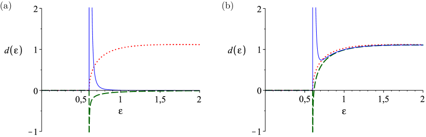
Figure 7: (a) The leading order density of states (dotted) along with the first (dashed) and second (solid) correction for $N=25$. (b) The leading order density of states (dotted) with the first (dashed) and then the second (solid) correction added for $N=25$.

The fact that the hard gap remains derives from the discriminant $D$ which is already present in $f$ (at $s=r^{2}=-1$) from (72). We could then expect that the gap is robust against further higher order corrections, seeing as the expressions always involve $f$. Someway above the gap we see that the corrections (especially the second) make little difference but it is the region directly above the gap which is particularly interesting. The expansion in inverse channel numbers is poorly (if at all) convergent but if the pattern of alternating singular peaks continues its sum (or rather the exact result for finite channel number) could take any value. In particular the gap could widen.

Though treating the density of states of Andreev billiards semiclassically basically just involves using different values for the variables in the graphical recursions, on the RMT side it remains to be seen how one could use recent advances, like the Selberg integral approach, to proceed beyond the leading order in inverse channel number. For the leading order [53] a diagrammatic expansion was performed, but a result for an arbitrary number of channels would be especially welcome. It would determine whether the gap indeed persists and would clarify what happens to the density of states just above the current gap.

5 Moments of the Wigner delay times

Another quantity related to the energy dependent correlation functions are the moments of the Wigner delay times. To obtain them we define the correlation function

$$D(\epsilon,n)=\frac{1}{N}\Tr\left[S^{\dagger}\left(E-\frac{\epsilon\hbar}{2\tau_{\mathrm{d}}}\right)S\left(E+\frac{\epsilon\hbar}{2\tau_{\mathrm{d}}}\right)-S^{\dagger}\left(E\right)S\left(E\right)\right]^{n},$$ (92)

where we subtract the identity matrix in the form of $S^{\dagger}S=I$. The corresponding generating function is

$$L(s)=\sum_{n=1}^{\infty}s^{n}D(\epsilon,n).$$ (93)

The moments of the Wigner-Smith matrix [54, 55]

$$Q=\frac{\hbar}{\rmi}S^{\dagger}(E)\frac{\rmd S(E)}{\rmd E},$$ (94)

are then given by [28]

$$m_{n}=\Tr\left[Q\right]^{n}=\frac{\tau_{\mathrm{d}}^{n}}{\rmi^{n}n!}\frac{\rmd^{n}}{\rmd\epsilon^{n}}D(\epsilon,n)\Big{|}_{\epsilon=0},$$ (95)

whose generating function we will denote

$$M(s)=\sum_{n=1}^{\infty}\frac{s^{n}}{\tau_{\mathrm{d}}^{n}}m_{n}.$$ (96)

The identity matrix in (92) follows by removing the $\epsilon$ dependence of the scattering matrices. However, as the identity matrix only has diagonal elements we identify these elements as diagonal trajectory pairs that travel directly from incoming to outgoing channels. We considered these to be formed when we moved encounters into the outgoing channels (equivalently we could use the incoming channels instead) whenever we formed an empty $\hat{f}$ subtree. The empty subtree is included in the general $\hat{f}$ contribution and we included the contribution $\sigma$ to allow us to change the effective value of $\hat{f}$ in this situation. The empty $\hat{f}$ subtrees consist of a single link and an incoming channel, producing the contribution $yc_{i}=r/(1-a)$. To mimic subtracting the identity matrix in (92) we simply take away the value of this empty subtree at zero energy ($a=0$) by setting

$$\sigma=-r,$$ (97)

along with the remaining semiclassical values in (69).

5.1 Subtrees

Including $\sigma$ breaks the symmetry of $f$ and $\hat{f}$, so the subtree recursions (5) and (6) become

$$\frac{f(1-a-f\hat{f})}{(1-f\hat{f})^{2}}=\frac{r}{(1+r^{2}-r\hat{f})},\qquad\frac{\hat{f}(1-a-f\hat{f})}{(1-f\hat{f})^{2}}=\frac{r}{(1-rf)},$$ (98)

and we find [28] that $f$ satisfies the following cubic

$$(1+r^{2})^{2}f^{3}-r(1+r^{2})(1+a)f^{2}-(1+r^{2})(1-a)f+r=0,$$ (99)

while $\hat{f}$ is related by

$$\hat{f}=(1+r^{2})f.$$ (100)

5.2 Leading order

For the energy dependent correlation functions we have

$$F_{0}=\frac{rNf}{1-rf}-\frac{r^{2}N}{(1+r^{2})(1-rf)}.$$ (101)

Setting $L_{0}=F_{0}/N$, inverting (101) and substituting into (72) we obtain the cubic

$$(1+s){L_{0}}^{3}+as(1+s){L_{0}}^{2}+s(2as+a-1){L_{0}}+as^{2}=0.$$ (102)

For the $n$-th moment of the delay times we want the coefficient of the $n$-th power of $a$ which we can extract by transforming $s\to s/a$ and then setting $a=0$. This leads to a quadratic and the leading order moment generating function [56, 28]

$$M_{0}(s)=\frac{1-s-\sqrt{1-6s+s^{2}}}{2}$$ (103)

Alternatively we can start with the generating function from (60)

$$\frac{K_{0}}{N} = \frac{1}{2}\ln(1-(1+r^{2})f^{2})+\frac{a(1+r^{2})f^{2}}{2(1-(1+r^{2})f^{2})}$$ (104)

$$-\frac{1}{2}\ln(1-rf)-\frac{1}{2}\ln\left[(1+r^{2})(1-rf)\right]$$

from which we can recover (102) and hence (103) by differentiating with respect to $r$, multiplying by $r$ and using the result for $\frac{\rmd f}{\rmd r}$ from differentiating (99) implicitly.

5.3 First orthogonal correction

For the first orthogonal correction we evaluate the contributions of the even and odd nodes around the Möbius strip

$$A(p)=\frac{h(h-p-2)}{(1-h)^{2}}+\frac{ah(h^{2}-3h+2p+4)}{(1-h)^{3}},$$ (105)

and

$$B(p)=\frac{pr^{2}}{(1+r^{2}-r\hat{f})(1-rf)}=\frac{ph(1-a-h)^{2}}{(1-h)^{4}},$$ (106)

which we again rewrite using (98) and both contributions only depend on $h=f\hat{f}$. Putting these contributions into the generating function (21) we again obtain

$$K_{1}=\frac{1}{4}\ln\left(\frac{(1+a)h^{2}-(2-a^{2})h+1-a}{(1+a)h^{2}-(2+a^{2})h+1-a}\right),$$ (107)

as in section 4.3 but with different values for $f$ and $\hat{f}$ as given in (99) and (100). Differentiating in line with (22) and differentiating (99) implicitly we arrive at the generating function, given as (157) in B, which generates the orthogonal correction to the correlation functions $D(\epsilon,n)$. Finally by transforming $s\to s/a$ and setting $a=0$ we find the correction to the moments of the delay times to be

$$NM_{1}(s)=\frac{1-3s-\sqrt{1-6s+s^{2}}}{2(1-6s+s^{2})}.$$ (108)

5.4 Next corrections

Since we only treated reflection quantities where $f=\hat{f}$ for the next order corrections we cannot obtain the corresponding generating functions of the moments of the delay times. Instead we can generate the energy dependent correlation functions $C(\epsilon,n)$ by expanding the generating function $G_{2}(s)$ which can be found by treating the six base cases as in section 4.4. Expanding to finite order, we can then obtain the functions $D(\epsilon,n)$ using the relation

$$D(\epsilon,n)=\sum_{k=0}^{n}\left(-1\right)^{n-k}{n\choose k}C(\epsilon,k),$$ (109)

which follows from the binomial expansion of (92) and where $C(\epsilon,0)=1$ has no subleading order contribution. Doing this only for the two base structures which exist without time reversal symmetry and plugging the resultant $D(\epsilon,n)$ into (95) we obtain the moments for the unitary case to low order. We find that the generating function

$$N^{2}M^{\mathrm{U}}_{2}(s)=\frac{2s^{2}}{(1-6s+s^{2})^{\frac{5}{2}}},$$ (110)

fits with these moments, while if we treat all six base structures, the generating function

$$N^{2}M^{\mathrm{O}}_{2}(s)=\frac{s(s-3)}{\left(1-6s+s^{2}\right)^{2}}+\frac{3s(s-1)^{2}+2s^{2}}{\left(1-6s+s^{2}\right)^{\frac{5}{2}}},$$ (111)

fits the low moments for systems with time reversal symmetry.

6 Cross correlation of transport moments

Along with transport moments, we can also consider non-linear statistics such as the cross correlation between transport moments, generated by

$$P_{[X_{1},X_{2}]}(s_{1},s_{2})=\sum_{n_{1},n_{2}=1}^{\infty}s_{1}^{n_{1}}s_{2}^{n_{2}}\left\langle\Tr[X_{1}^{\dagger}X_{1}]^{n_{1}}\Tr[X_{2}^{\dagger}X_{2}]^{n_{2}}\right\rangle,$$ (112)

which involves two traces inside the energy average. Semiclassically we then have an expression involving two trajectory sets that form two separate cycles, as in figure 8(a). Of course when we look for trajectory sets which lead to a small action difference we can have independent diagrams for each set, as in figure 8(b). However, these are included in the individual moments treated previously, and when we remove them,

$$\tilde{P}_{[X_{1},X_{2}]}(s_{1},s_{2})=P_{[X_{1},X_{2}]}(s_{1},s_{2})-\sum_{n_{1},n_{2}=1}^{\infty}s_{1}^{n_{1}}s_{2}^{n_{2}}\left\langle\Tr[X_{1}^{\dagger}X_{1}]^{n_{1}}\right\rangle\left\langle\Tr[X_{2}^{\dagger}X_{2}]^{n_{2}}\right\rangle,$$ (113)

we are left with trajectories that must interact, as in figure 8(c). In RMT, this quantity is known as the ‘connected’ part of the correlation function.

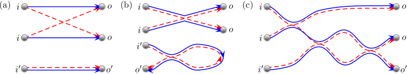
Figure 8: (a) With two traces, the semiclassical trajectories separate into two closed cycles. When the two sets do not interact as in (b) we recreate terms from $\left\langle\Tr[X_{1}^{\dagger}X_{1}]^{n_{1}}\right\rangle\left\langle\Tr[X_{2}^{\dagger}X_{2}]^{n_{2}}\right\rangle$, but when they do interact as in (c) further diagrams are possible as in figure 9.

It is interesting to consider the combinatorial interpretation of the interacting sets of trajectories. Denote the incoming channels belonging to the first trace by $i_{j}$, $j=1,\ldots,n_{1}$ and the incoming channels from the second trace by $i_{j}^{\prime}$, $j=1,\ldots,n_{2}$. Input channels are mapped onto output channels by trajectories from $X$ and also by trajectories from $X^{\dagger}$. If we apply the first mapping followed by the inverse of the second mapping, we end up with the following transitions

$$i_{1}\mapsto i_{2},\ \ldots\ i_{n_{1}}\mapsto i_{1},\qquad\mbox{and}\qquad i_{1}^{\prime}\mapsto i_{2}^{\prime},\ \ldots\ i_{n_{2}}^{\prime}\mapsto i_{1}^{\prime}.$$ (114)

Thus the overall result is a permutation, written in the cycle notation as $\pi=(i_{1}\ \ldots\ i_{n_{1}})(i_{1}^{\prime}\ \ldots\ i_{n_{2}}^{\prime})$. We can interpret each $l$-encounter as a cycle permuting $l$ labels of the corresponding $X$ trajectories. Then an entire leading order diagram can be interpreted as a factorization of $\pi$ into smaller cycles (c.f. [57]). In the language of combinatorics, interacting trajectories correspond to a transitive factorization, leading order corresponds to the minimality condition and the fact that encounters on different ‘branches’ have no ordering imposed on them corresponds to counting inequivalent factorizations (up to a permutation of commuting factors). To summarize, the leading order interacting diagrams are in one-to-one correspondence with the minimal transitive inequivalent factorizations of a permutation into smaller cycles. This question has been studied combinatorially (for factorizations into transpositions only) for a permutation consisting of two cycles in [58] and for three and more cycles (these correspond to 3-point and higher cross correlations) in [59, 60]. We note that the above combinatorial questions and the evaluation of transport properties are not completely equivalent problems. To evaluate transport properties we need to find additional information regarding the number of encounters touching the lead. On the other hand, we make substitutions (8) or (13) which significantly simplify the results.

6.1 Leading order

We now proceed to expand the contributions of the interacting sets of trajectories in inverse powers of the total channel number by describing the corresponding graphical representations. The base diagram for the leading order term is just a single loop, like in figure 4(d) except with no twist. Without the twist, the two cycles of the permutation arise from the two walks on the inside and outside of the loop, see figure 9(a). One requirement, to ensure a small action difference, is that the parts of the loop are traversed on either side by parts of trajectories that contribute actions with different signs in the semiclassical expression. In figure 9 this means that the (blue) solid or dashed dotted lines on either side of the loop must partner (red) dashed or dotted lines on the other. Without time reversal symmetry the parts of the loop must additionally be traversed in the same direction by trajectory stretches and their partners, so that at odd nodes (those with an odd number of subtrees on each side of the loop) there is unequal number of channels of a given type, as in figure 9(a). With time reversal symmetry, parts of the loop may be traversed in any direction and we may also swap all the incoming and outgoing directions on one side (the inside say) of the loop as in figure 9(b).

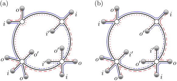
Figure 9: Example graphs, which contribute to the leading order in inverse channel number of $\tilde{P}_{[X_{1},X_{2}]}(s_{1},s_{2})$, made out of a single loop with subtrees attached at nodes. For a small action difference, the (blue) solid or dashed dotted lines must partner (red) dashed or dotted lines on the other side of the loop. (a) Without time reversal symmetry the odd nodes have either incoming or outgoing channels on the outer subtrees on each side of the loop. (b) With time reversal symmetry we may also swap the incoming and outgoing channels inside the loop.

With these restrictions we can start to append subtrees at nodes around the loop. We will use the tree function $f_{1}$ and generating variable $\rho_{1}$ for the subtrees outside the loop and $f_{2}$ and $\rho_{2}$ for those inside. At each node we can either add an even or odd number of subtrees on each side of the loop and we start with the contribution when we add an even number

$$A^{\mathrm{even}}=\sum_{l=2}^{\infty}x_{l}\sum_{k=0}^{l-1}h_{1}^{k}h_{2}^{(l-1-k)}=\sum_{l=2}^{\infty}x_{l}\frac{h_{1}^{l}-h_{2}^{l}}{h_{1}-h_{2}},$$ (115)

where $h_{1}=f_{1}\hat{f}_{1}$.

For systems without time reversal symmetry, with an odd number of subtrees on each side (an odd node) we have two possibilities as in figure 9(a). The subtrees in the odd positions on both sides all connect (first and last) to either incoming or outgoing channels. With outgoing channels we have the contribution

$$A^{\mathrm{odd}}_{\mathrm{a},o}=\sum_{l=2}^{\infty}x_{l}\sum_{k=1}^{l-1}f_{1}h_{1}^{k-1}f_{2}h_{2}^{(l-1-k)}=\sum_{l=2}^{\infty}x_{l}f_{1}f_{2}\frac{h_{1}^{l-1}-h_{2}^{l-1}}{h_{1}-h_{2}},$$ (116)

while with incoming channels we swap $f$ with $\hat{f}$

$$A^{\mathrm{odd}}_{\mathrm{a},i}=\sum_{l=2}^{\infty}x_{l}\hat{f}_{1}\hat{f}_{2}\frac{h_{1}^{l-1}-h_{2}^{l-1}}{h_{1}-h_{2}}.$$ (117)

As before it is possible that an odd node touches the lead when the odd positioned subtrees on both sides are empty. Of course this also requires that the incoming or outgoing channels of the two quantities $X_{1}$ and $X_{2}$ originate or end in the same lead. When this is the case, we also have the following contribution

$$B_{\mathrm{a},o} = \sum_{l=2}^{\infty}\frac{z_{o,l}}{r^{l}}\sum_{k=1}^{l-1}\rho_{1}^{k}\hat{f}_{1}^{k-1}\rho_{2}^{l-k}\hat{f}_{2}^{(l-k-1)}$$

$$= \sum_{l=2}^{\infty}\frac{z_{o,l}}{r^{l}}\rho_{1}\rho_{2}\frac{(\rho_{1}\hat{f}_{1})^{l-1}-(\rho_{2}\hat{f}_{2})^{l-1}}{\rho_{1}\hat{f}_{1}-\rho_{2}\hat{f}_{2}},$$

where we needed to include the explicit $\rho_{1}$ and $\rho_{2}$ dependence of $\boldsymbol{z}_{o}$ on the number of empty trees on each side of the loop. With incoming channels instead we again swap $f$ and $\hat{f}$

$$B_{\mathrm{a},i}=\sum_{l=2}^{\infty}\frac{z_{i,l}}{r^{l}}\rho_{1}\rho_{2}\frac{(\rho_{1}f_{1})^{l-1}-(\rho_{2}f_{2})^{l-1}}{\rho_{1}f_{1}-\rho_{2}f_{2}}.$$ (119)

We allow an arbitrary number, $k$, of nodes along the loop, but the total number of odd nodes must be even. Taking into account rotational symmetry, we get

$$\tilde{\kappa}_{1\mathrm{a}}=-\ln\left[1-yZ_{\mathrm{a}}(p)\right],$$ (120)

where $Z_{\mathrm{a}}(p)$ is a contribution of one node. The node can either be even or odd of one of two types. Since the number of odd $i$-nodes is equal to the number of odd $o$-nodes, we can write $Z_{\mathrm{a}}(p)$ as

$$Z_{\mathrm{a}}(p)=A^{\mathrm{even}}+p\sqrt{(A^{\mathrm{odd}}_{\mathrm{a},i}+B_{\mathrm{a},i})(A^{\mathrm{odd}}_{\mathrm{a},o}+B_{\mathrm{a},o})}.$$ (121)

To ensure that we indeed have an even number of odd nodes, we set

$$\kappa_{1}=\frac{\tilde{\kappa}_{1}(p=1)+\tilde{\kappa}_{1}(p=-1)}{2},$$ (122)

leading to

$$\kappa_{1\mathrm{a}}=-\frac{1}{2}\ln\left[(1-yA^{\mathrm{even}})^{2}-y^{2}(A^{\mathrm{odd}}_{\mathrm{a},i}+B_{\mathrm{a},i})(A^{\mathrm{odd}}_{\mathrm{a},o}+B_{\mathrm{a},o})\right].$$ (123)

For the additional contribution, in the case of systems with time reversal symmetry, from the diagrams like figure 9(b) we swap the incoming and outgoing channels inside the loop so that we now have the contributions

$$A^{\mathrm{odd}}_{\mathrm{b},o}=\sum_{l=2}^{\infty}x_{l}\hat{f}_{1}f_{2}\frac{h_{1}^{l-1}-h_{2}^{l-1}}{h_{1}-h_{2}},\qquad A^{\mathrm{odd}}_{\mathrm{b},i}=\sum_{l=2}^{\infty}x_{l}f_{1}\hat{f}_{2}\frac{h_{1}^{l-1}-h_{2}^{l-1}}{h_{1}-h_{2}},$$ (124)

and

$$B_{\mathrm{b},o} = \sum_{l=2}^{\infty}\frac{z_{o,l}}{r^{l}}\rho_{1}\rho_{2}\frac{(\rho_{1}f_{1})^{l-1}-(\rho_{2}\hat{f}_{2})^{l-1}}{\rho_{1}f_{1}-\rho_{2}\hat{f}_{2}},$$ (125)

$$B_{\mathrm{b},i} = \sum_{l=2}^{\infty}\frac{z_{i,l}}{r^{l}}\rho_{1}\rho_{2}\frac{(\rho_{1}\hat{f}_{1})^{l-1}-(\rho_{2}f_{2})^{l-1}}{\rho_{1}\hat{f}_{1}-\rho_{2}f_{2}},$$

and correspondingly

$$\kappa_{1\mathrm{b}}=-\frac{1}{2}\ln\left[(1-yA^{\mathrm{even}})^{2}-y^{2}(A^{\mathrm{odd}}_{\mathrm{b},i}+B_{\mathrm{b},i})(A^{\mathrm{odd}}_{\mathrm{b},o}+B_{\mathrm{b},o})\right].$$ (126)

There is also an additional freedom of placing the label $i_{1}$ on any leaf outside, giving a factor of $2n_{1}$. Once $i_{1}$ has been placed the type (in- or out-) of the leaves inside is fixed and the freedom of placing the label $i_{1}^{\prime}$ inside produces only a factor of $n_{2}$. We obtain these factors by differentiating with respect to the variables $\rho_{1}$ and $\rho_{2}$,

$$\Gamma=\frac{\rho_{1}\rho_{2}}{2}\frac{\partial^{2}\kappa}{\partial\rho_{1}\partial\rho_{2}}.$$ (127)

We further note that the differentiation ensures that there are at least two channels both inside and outside the loop.

Using the appropriate semiclassical values of the variables $\boldsymbol{x}$, $\boldsymbol{z}$ and $y$ as well as the corresponding subtree contributions, we find the following generating functions

$$\tilde{P}_{[r_{1},r_{1}],1}^{\mathrm{U}}(s_{1},s_{2})=\tilde{P}_{[r_{1},r_{2}],1}^{\mathrm{U}}(s_{1},s_{2})=\frac{s_{1}s_{2}}{2\left(s_{1}-s_{2}\right)^{2}}\left[\frac{1-2\xi\left(s_{1}+s_{2}\right)}{\sqrt{1-4\xi s_{1}}\sqrt{1-4\xi s_{2}}}-1\right],$$ (128)

with $s_{1}=\rho_{1}^{2}$ and $s_{2}=\rho_{2}^{2}$ and twice this result for the orthogonal case with time reversal symmetry. Even though for the autocorrelation $\tilde{P}_{[r_{1},r_{1}],1}^{\mathrm{U}}$ we can always move the odd nodes into the lead while for the cross correlation $\tilde{P}_{[r_{1},r_{2}],1}^{\mathrm{U}}$ we can not, this is somehow compensated for by the different subtree contributions and both give the same result.

For the transmission autocorrelation we can move the odd nodes into the lead only for the unitary diagrams, leading to the generating function

$$\tilde{P}_{[t,t],1}^{\mathrm{U}}(s_{1},s_{2})=\frac{s_{1}s_{2}}{2\left(s_{1}-s_{2}\right)^{2}}\left[\frac{1+\left(2\xi-1\right)\left(s_{1}+s_{2}\right)+\left(1-4\xi\right)s_{1}s_{2}}{(1-s_{1})\sqrt{1+\frac{4\xi s_{1}}{1-s_{1}}}(1-s_{2})\sqrt{1+\frac{4\xi s_{2}}{1-s_{2}}}}-1\right],$$ (129)

and we still obtain twice this for the orthogonal result. Finally for the cross correlation between the reflection and transmission we have

$$\tilde{P}_{[r_{1},t],1}^{\mathrm{U}}(s_{1},s_{2})=\frac{s_{1}s_{2}}{2\left(s_{1}-s_{1}s_{2}+s_{2}\right)^{2}}\left[1-\frac{1-s_{2}+2\xi\left(s_{2}-s_{1}+s_{1}s_{2}\right)}{\sqrt{1-4\xi s_{1}}(1-s_{2})\sqrt{1+\frac{4\xi s_{2}}{1-s_{2}}}}\right],$$ (130)

and twice this for the orthogonal case. Note that the above results remain unchanged if we swap $r_{1}$ and $r_{2}$ as this just means swapping $\zeta_{1}$ and $\zeta_{2}$ in the semiclassical contributions which does not change $\xi$. From these results we can obtain the corresponding $P_{[X_{1},X_{2}]}$ up to the first subleading order by including the first three orders in inverse channel number of the moments corresponding to $X_{1}$ multiplied by the moments corresponding to $X_{2}$. If we also include $n=0$ terms (which are just the number of channels in the respective lead) with those moments then we obtain the $n_{1}=0$ and $n_{2}=0$ terms in (112). This then allows us to check that expansions of the various transport correlation functions indeed fulfil the unitarity conditions in (2). Note that if we assume a priori that the unitarity is preserved by the semiclassical approximation (3), any one of equations (128)–(130) implies all others.

6.2 Subleading correction

We can continue this process and look at the base structures like in figures 5 and 6 but which separate into two cycles. In fact the possibilities are almost the same as in figure 6 but with one twist more or fewer as depicted in figure 10. These can also exist only for systems with time reversal symmetry and we can treat them in a similar way as before, but with the modifications above.

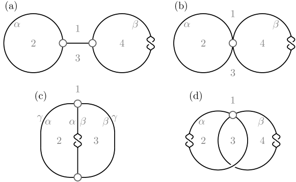
Figure 10: The base structures which break into two cycles (for systems with time reversal symmetry) at the second subleading order in inverse channel number.

Again the types of subtrees at each node depends on the nodes elsewhere in the diagram, so we restrict out attention to the simpler case of the reflection where $f=\hat{f}$. Because of (2), we have

$$\Tr[r_{1}^{\dagger}r_{1}]^{n}-N_{1}=\sum_{k=1}^{n}(-1)^{k}{n\choose k}\Tr[t^{\dagger}t]^{k}=\Tr[r_{2}^{\dagger}r_{2}]^{n}-N_{2},$$ (131)

so that $\tilde{P}_{[r_{1},r_{1}]}=\tilde{P}_{[r_{1},r_{2}]}$ where the reflection autocorrelation is equal to the reflection cross correlation. However for the cross correlation, as the channels of the two reflections are in different leads, the nodes which lie on both cycles can not enter the lead, and this further simplifies the calculation. The edges which travel through both cycles then provide factors

$$\eta(p)=\frac{1}{1-(A^{\mathrm{even}}+pA^{\mathrm{odd}})},$$ (132)

while the edges which only pass through one cycle provide factors $E(p)$ as before, but with the semiclassical values corresponding to the reflection into lead 1 or lead 2 as appropriate. We will denote this correspondence by a subscript in the following.

The treatment of the diagrams is very similar to that in section 3.3 so we merely highlight the steps here. But first we discuss the symmetry factors. Because of time-reversal symmetry, we can put the first incoming channels on both faces on any leaf, leading to the differential operator $\rho_{1}\rho_{2}\frac{\partial^{2}\kappa}{\partial\rho_{1}\partial\rho_{2}}$. Unlike the diagrams in figure 9, the ‘inside’ and ‘outside’ faces are, in general, not related by symmetry, and we should consider both putting $f_{1}$-trees on the ‘outside’ and on the ‘inside’. For brevity we will only list the former contributions. Finally, the symmetry groups of diagrams 10(c) and 10(d) have order $2$ and $4$ correspondingly and we will divide their contributions by the appropriate factor.

Starting with the diagram in figure 10(a), for the node on the left, which cannot enter the lead, we have

$$\tilde{\nu}_{3\mathrm{a}}(q)=-\sum_{k_{1},k_{2},k_{3}=0}^{\infty}(qf_{1})^{(k_{1}+k_{3})}(qf_{2})^{k_{2}}p_{\alpha}^{k_{2}},$$ (133)

with an odd number of trees appended

$$\nu_{3\mathrm{a}}=\frac{\tilde{\nu}_{3\mathrm{a}}(q=1)-\tilde{\nu}_{3a}(q=-1)}{2}.$$ (134)

For the node on the right we have $\hat{V}_{3\mathrm{a}}$ as before but with semiclassical values corresponding to the reflection into lead 1. To ensure a valid semiclassical diagram we still need each cycle to contain an even number of objects, so we have

$$\tilde{\kappa}^{\mathrm{O}}_{2\mathrm{a}}=p_{\beta}\eta(p_{\alpha})E_{1}(1)E_{1}(p_{\beta})\nu_{3\mathrm{a}}\hat{V}_{3\mathrm{a}}.$$ (135)

This is then averaged

$$\kappa^{\mathrm{O}}_{2\mathrm{a}}=\frac{\tilde{\kappa}^{\mathrm{O}}_{2\mathrm{a}}(p=1)+\tilde{\kappa}^{\mathrm{O}}_{2\mathrm{a}}(p=-1)}{2},$$ (136)

for $p_{\alpha}$ and $p_{\beta}$ in turn. Finally, we add the contribution where we place $f_{1}$ subtrees along the inside and $f_{2}$ subtrees along the outside. For the reflection cross correlation this reduces to swapping $\rho_{1}$ with $\rho_{2}$ and swapping $\zeta_{1}$ with $\zeta_{2}=1-\zeta_{1}$.

The node in figure 10(b) gives

$$\tilde{\nu}_{4\mathrm{b}}(q)=-\sum_{k_{1},k_{2},k_{3},k_{4}=0}^{\infty}(qf_{1})^{(k_{1}+k_{3}+k_{4})}(qf_{2})^{k_{2}}p_{\alpha}^{k_{2}}p_{\beta}^{k_{4}},$$ (137)

with an even number of subtrees in total

$$\nu_{4\mathrm{b}}=\frac{\tilde{\nu}_{4\mathrm{b}}(q=1)+\tilde{\nu}_{4\mathrm{b}}(q=-1)}{2},$$ (138)

The total contribution is then

$$\tilde{\kappa}^{\mathrm{O}}_{2\mathrm{b}}=p_{\beta}\eta(p_{\alpha})E_{1}(p_{\beta})\nu_{4\mathrm{b}}.$$ (139)

averaged over $p_{\alpha}$ and $p_{\beta}$ in turn and we again add the result where we swap the trees on the inside and the outside.

For the structure in figure 10(c) the nodes provide

$$\tilde{\nu}_{3\mathrm{c}}(q)=-\sum_{k_{1},k_{2},k_{3}=0}^{\infty}(qf_{1})^{k_{1}}(qf_{2})^{(k_{2}+k_{3})}p_{\alpha}^{k_{2}}p_{\beta}^{k_{3}}p_{\gamma}^{k_{1}},$$ (140)

with

$$\nu_{3\mathrm{c}}=\frac{\tilde{\nu}_{3\mathrm{c}}(q=1)-\tilde{\nu}_{3c}(q=-1)}{2},$$ (141)

so that the contribution is then

$$\tilde{k}^{\mathrm{O}}_{2\mathrm{c}}=\frac{1}{2}p_{\alpha}p_{\beta}E_{2}(p_{\alpha}p_{\beta})\eta(p_{\beta}p_{\gamma})\eta(p_{\gamma}p_{\alpha})(\nu_{3\mathrm{c}})^{2}$$ (142)

before averaging over the $p$’s in turn. Likewise we include the contribution where we swap the subtrees on the inside with those on the outside.

Finally the node in figure 10(d) provides

$$\tilde{\nu}_{4\mathrm{d}}(q)=-\sum_{k_{1},k_{2},k_{3},k_{4}=0}^{\infty}(qf_{1})^{(k_{1}+k_{3})}(qf_{2})^{(k_{2}+k_{4})}p_{\alpha}^{k_{2}}(p_{\alpha}p_{\beta})^{k_{3}}p_{\beta}^{k_{4}},$$ (143)

with

$$\nu_{4\mathrm{d}}=\frac{\tilde{\nu}_{4\mathrm{d}}(q=1)+\tilde{\nu}_{4\mathrm{d}}(q=-1)}{2}.$$ (144)

The total contribution is then

$$\tilde{\kappa}^{\mathrm{O}}_{2\mathrm{d}}=\frac{1}{4}\eta(p_{\alpha})\eta(p_{\beta})\nu_{4\mathrm{d}},$$ (145)

averaged over $p_{\alpha}$ and $p_{\beta}$ in turn. We also include the contribution where we swap the subtrees on the inside and outside.

Summing the four diagrams, we eventually arrive at the generating function

$$N\tilde{P}_{[r_{1},r_{2}],2}^{\mathrm{O}}(s_{1},s_{2}) = \left[s_{1}+s_{2}-2s_{1}s_{2}-2\xi\left(4s_{1}^{2}+s_{2}^{2}+3s_{1}s_{2}-s_{1}^{3}-5s_{1}^{2}s_{2}-2s_{1}s_{2}^{2}\right)\right.$$ (146)

$$\qquad\left.{}+8s_{1}^{2}\xi^{2}\left(s_{1}+3s_{2}-3s_{1}s_{2}-s_{2}^{2}\right)\right]$$

$$\times\frac{s_{1}s_{2}}{(s_{1}-s_{2})^{3}(1-4\xi s_{1})^{2}\sqrt{1-4\xi s_{2}}}+\left(s_{1}\leftrightarrow s_{2}\right),$$

where $\left(s_{1}\leftrightarrow s_{2}\right)$ means we add the result with $s_{1}$ and $s_{2}$ swapped.

We could check that the results in this section all agree with the first four moments calculated from the arbitrary channel RMT results of [12].

7 Conclusions and discussion

We described a method for the semiclassical calculation of the expansion of several transport statistics asymptotically in the inverse channel number $1/N$. The calculation is performed by grafting trees onto the base structures with a low number of cycles, and relies on the fact that attaching trees does not change the order in inverse channel number. Instead, the trees add more incoming and outgoing channels and so increase the order of the moment. With graphical recursions, this allows us to generate all the moments at a given order in inverse channel number, which we performed up to the third order. The terms we considered suggest the following observations about the ribbon graphs that arise as the contributing diagrams

• absence of time reversal symmetry results in graphs being orientable; both orientable and non-orientable graphs contribute to the calculation with time reversal symmetry,

• the order (in $1/N$) of a contribution is reflected in the genus of the corresponding graph,

• linear moments (with one trace) result in graphs with one face, while non-linear moments with $m$ traces will require considering graphs with $m$ faces.

The above general observations suggest that a complete expansion in $1/N$ should be both feasible and interesting to specialists working in algebra and combinatorics.

We find that the semiclassical contribution of individual base diagrams depends significantly on the global structure of the diagram. This is in contrast to the expansions of the first two moments performed in [25, 11, 26], where the contribution factorized into a product over the vertices of the diagram and the problem was thus reduced to a combinatorial enumeration. The latter was achieved through finding recursion relations which connect different diagrams, and similar ideas could well be useful for the base structures we need for all moments. To illustrate the scale of the problem of going to higher order in $1/N$, for the unitary case there are 1848 base diagrams at the next contributing order. As they can involve more than two nodes, they can no longer be derived by cleaning the corresponding semiclassical conductance diagrams as was the case for the orders treated in this article. However, in the end all these diagrams would probably lead to the generating functions (149) and (153), highlighting the scale of the simplifications that take place.

Our results fully agree with the predictions of RMT theory (as far as those are available [15]), and importantly are given in terms of very simple generating functions. This would suggest that extending the types of asymptotic analyses of [47, 48, 49] beyond the leading order, (as is currently being performed [15]), one could also expect to see simplifications of the RMT results. For the unitary case, where several different formulae are known for the moments of the transmission eigenvalues [13, 14, 15, 16], this analysis and the semiclassical endpoints could shed light on the combinatorial relationships between the different approaches. Because of the connection between RMT and weakly disordered systems, we can expect that our results also apply to such systems. Likewise, with the close correspondence between semiclassical and disorder diagrams [43], one might hope to find similar graphical recursions in a perturbative expansion of the appropriate nonlinear $\sigma$ model.

If we were to consider non-linear statistics involving three traces (with their mean parts removed), the leading contribution would come from the diagrams like in figures 6 and 10 which split into three cycles, i.e. diagrams (a)–(c) without any twists. Considering quantities with $m$ traces we would then need to treat base diagrams related to those which contribute to order $1/N^{(m-2)}$ (and higher) for the linear statistics, and so we immediately run into the considerations and difficulties described above. Curiously though the moments of the conductance and the shot noise themselves can be efficiently treated using RMT [14, 17, 18, 19]. Semiclassically, the $m$-th moment of these quantities corresponds to having exactly 2 or 4 channels along each of the $m$ cycles, and the RMT results might then provide a pathway for generating such semiclassical diagrams. This could in turn be useful for generating and treating the corresponding base diagrams for the linear statistics.

The methods described in this article were also used to treat the density of states of Andreev billiards. Replacing the normal conducting leads of the chaotic cavity by a superconductor produces strong effects like the complete suppression of the density of states around the Fermi energy [53, 29, 30]. Being interested in the density of states one must evaluate moments of all orders, something that our methods are particularly geared towards. Going beyond leading order in inverse channel number we could show that this gap persists for the next two orders, and that the behaviour of the density of states slightly above the gap is not determined by just these terms in the expansion. Because of the superconductor, one not only needs to know all the moments but also all the higher orders in inverse channel number. A result for arbitrary channel number would therefore be particularly welcome for such systems, which leads to the question of how to adapt the recent RMT advances to tackle this problem. Similarly, chaotic cavities with additional superconductors attached (Andreev dots) also exhibit significant effects due to the presence of the superconductors and also require one to be able to treat what would correspond to all the moments of usual transport quantities. For example, at leading order in inverse channel number, the conductance through a normal chaotic cavity requires just the diagonal pair of trajectories, while for the conductance through an Andreev dot one needs full tree recursions [32]. The treatment is actually similar to the edges in the base diagrams here, but with the added ingredient of having two (or more) different species of subtree. One can then see that treating the transport moments of Andreev dots requires an extra layer of complexity compared to normal chaotic cavities.

The results in this article are all for the case in which the leads are perfectly coupled to the chaotic cavity, rather than for the more general and experimentally relevant case of non-ideal coupling. This is typically modelled by introducing tunnel barriers into the leads with some probability to backscatter when entering (or leaving) the cavity. Semiclassically, along with affecting the contributions of the channels and modifying the survival probability and hence contributions of the links and the correlated trajectory stretches inside the encounters, the main change is that a wealth of new diagrams become possible [61]. Specifically, encounters may now partially touch the leads and have some of their links backreflected at the tunnel barrier while the rest tunnel through to enter or exit the system. In principle, these possibilities would become extra terms in the tree and graphical recursions in this article, but so far these types of diagrams have only been treated semiclassically for the lowest moments [61, 62]. However, from a RMT viewpoint at leading order in inverse channel number and with the same tunnelling probability for each channel, the non-ideal contacts just increase the order of the generating functions by one, for example for both the density of states of Andreev billiards [53] and the moments of the Wigner delay times [63].

Finally one can wonder whether the effect of the Ehrenfest time can be incorporated into the graphical recursions developed here. For the leading order in inverse channel number, the effect could be included [33] in the tree recursions. First, the trees are related to each other through a continuous deformation, for example by giving the nodes a certain size (actually, the Ehrenfest time itself) and allowing them to slide into each other. Second, this is then partitioned in a particular way so that one can extract the Ehrenfest time dependence efficiently. Each partition and hence the sum of all diagrams leads to the same simple Ehrenfest time dependence at leading order in inverse channel number [33] and this pattern and treatment seems to also hold at the first subleading order [64]. Whether this continues to higher order and nonlinear statistics, which start to include the complications of periodic orbit encounters, is an intriguing question.

Appendix A Unitary reflection and transmission

Using the RMT result from [14] we can compute the moments up to finite order and expand them in powers of the inverse channel number. Looking at the patterns for the reflection in (62), (29) and (41), we can expect that each order in the inverse channel number just increases the powers in the denominators (the square root comes simply from the subtrees). In fact we find that the first several subleading orders can be written as

$$N^{2k-1}R_{2k}(s)=\frac{\xi^{2}s^{2}(s-1)}{(1-4\xi s)^{\frac{6k-1}{2}}}\cdot\boldsymbol{\chi}_{2k-1}X_{2k-1}\boldsymbol{S}_{2k-1}^{\mathrm{T}}$$ (147)

where $\boldsymbol{\chi}_{m}$ is the vector $(1,\xi s,\xi^{2}s^{2},\ldots,\xi^{m-1}s^{m-1})$, $X_{m}$ is an $m\times m$ matrix and $\boldsymbol{S}_{m}$ is the row vector $(1,s,s^{2},\ldots,s^{m-1})$. The first few values of $X_{m}$ are

$$X_{1}=(1)$$ (148)

$$X_{3}=\left(\begin{array}[]{ccc}1&-8&8\\ 20&-20&-8\\ 9&-2&9\end{array}\right)$$ (149)

$$X_{5}=\left(\begin{array}[]{ccccc}1&-40&220&-360&180\\ 136&-1240&2480&-1360&-32\\ 1770&-5700&4890&-1392&528\\ 3080&-4760&1736&408&-720\\ 450&-360&76&-360&450\end{array}\right)$$ (150)

$$X_{7}=\left(\small{\begin{array}[]{ccccccc}1&-168&2688&-13104&26712&-24192&8064\\ 636&-19068&125832&-313824&342048&-151200&15552\\ 34659&-401142&1357755&-1917888&1210608&-326496&42744\\ 398328&-2303784&4455864&-3638040&1157712&5952&-77312\\ 1152438&-3903144&4477620&-1989144&322326&-186288&130032\\ 766584&-1652952&1107456&-238704&-35400&172872&-126000\\ 55125&-78750&28539&-5732&28539&-78750&55125\end{array}}\right)$$

Similarly we can write the transmission as

$$N^{2k-1}T_{2k}(s)=-\frac{\xi^{2}s^{2}}{(1-s)^{\frac{2k+1}{2}}(1-s+4\xi s)^{\frac{6k-1}{2}}}\cdot\boldsymbol{\upsilon}_{2k-1}Y_{2k-1}\boldsymbol{S}_{2k-1}^{\mathrm{T}}$$ (151)

where $\boldsymbol{\upsilon}_{m}$ is the vector $((1-s)^{m-1},\xi s(1-s)^{m-2},\xi^{2}s^{2}(1-s)^{m-3},\ldots,\xi^{m-1}s^{m-1})$ and $\boldsymbol{S}_{m}$ is the row vector $(1,s,s^{2},\ldots,s^{m-1})$. The first few values of the matrix $Y_{m}$ are

$$Y_{1}=(1)$$ (152)

$$Y_{3}=\left(\begin{array}[]{ccc}1&6&1\\ -20&20&8\\ 9&-16&16\end{array}\right)$$ (153)

$$Y_{5}=\left(\begin{array}[]{ccccc}1&36&106&36&1\\ -136&-696&424&424&16\\ 1770&-1380&-1590&1632&96\\ -3080&7560&-5936&1920&256\\ 450&-1440&1696&-512&256\end{array}\right)$$ (154)

$$Y_{7}=\left(\small{\begin{array}[]{ccccccc}1&162&1863&4012&1863&162&1\\ -636&-15252&-40032&11544&25572&3228&24\\ 34659&193188&-128070&-194892&111939&25680&240\\ -398328&86184&1088136&-885864&84144&101760&1280\\ 1152438&-3011484&2248470&61344&-524256&199680&3840\\ -766584&2946552&-4341456&2993280&-862464&150528&6144\\ 55125&-252000&461664&-423424&221952&-12288&4096\end{array}}\right)$$

Similar patterns hold for the moments of the delay times for the unitary case, and the results are actually simpler than for the transmission and reflection since there is one parameter fewer. The likely generating functions can be found by expanding the RMT result of [15] and fitting to the behaviour of (103) and (110).

Appendix B Further generating functions

For the energy dependent correlation functions, we find that the generating function $G_{1}=F_{1}/N$ satisfies the cubic

$$0 = \left[4(1-a)^{3}+s(a^{4}-20a^{2}-8)+4s(a+1)^{3}\right]^{2}(NG_{1})^{3}$$ (155)

$${}+2\left[(a-1)^{3}+s^{2}(a+1)^{3}\right]\left[4(1-a)^{3}+s(a^{4}-20a^{2}-8)+4s^{2}(a+1)^{3}\right](NG_{1})^{2}$$

$${}+\left[(a-1)^{6}-4s(a+1)(a-1)^{4}+3s^{2}(a-1)(a+1)(a^{4}-8a^{2}-2)\right.$$

$${}\qquad\left.+4s^{3}(a-1)(a+1)^{4}+s^{4}(a+1)^{6}\right]NG_{1}$$

$${}+a^{2}s\left[(a-1)^{3}+s^{2}(a+1)^{3}\right],$$

while the energy differentiated generating function instead satisfies

$$0 = a^{2}\left[4(1-a)^{3}+s(a^{4}-20a^{2}-8)+4s^{2}(a+1)^{3}\right]^{2}(NH_{1})^{3}$$ (156)

$${}+2a\left[(4-a)(a-1)^{2}-2s(5a^{2}+4)+s^{2}(a+4)(a+1)^{2}\right]$$

$${}\qquad\times\left[4(1-a)^{3}+s(a^{4}-20a^{2}-8)+4s^{2}(a+1)^{3}\right](NH_{1})^{2}$$

$${}+\left[(a-4)^{2}(a-1)^{4}+4s(a-1)^{2}(6a^{3}-21a^{2}+4a-16)\right.$$

$${}\qquad+s^{2}(-3a^{6}+156a^{4}+102a^{2}+96)$$

$${}\qquad\left.-4s^{3}(a+1)^{2}(6a^{3}-21a^{2}+4a-16)+s^{4}(a+4)^{2}(a+1)^{4}\right]NH_{1}$$

$${}+as(s-1)\left[(a+2)(a-4)^{2}+s(a-2)(a+4)^{2}\right].$$

For the moments of the delay times we have the first subleading order generating function

$$0 = (s+1)^{2}\left[4(1-a)^{3}+sa(a^{3}-8a^{2}+4a-24)+s^{2}a^{2}(a^{2}+4)\right]^{2}(NL_{1})^{3}$$ (157)

$${}+2(s+1)\left[(a-1)^{3}+2s(a-1)^{3}+2s^{2}a(a^{2}+3)\right]$$

$${}\qquad\times\left[4(1-a)^{3}+sa(a^{3}-8a^{2}+4a-24)+s^{2}a^{2}(a^{2}+4)\right](NL_{1})^{2}$$

$${}+\left[(a-1)^{6}+4sa(a-3)(a-1)^{4}+3s^{2}a^{2}(a-1)(3a^{3}-13a^{2}+20a-28)\right.$$

$${}\qquad\left.+2s^{3}a^{2}(a-1)(5a^{3}-11a^{2}+16a-32)^{4}+s^{4}a^{2}(5a^{4}+27a^{2}+32)\right]NL_{1}$$

$${}+sa^{2}\left[(a-1)^{3}+2s(a-1)^{3}+2s^{2}a(a^{2}+3)\right].$$

References

References

- [1] R. Landauer 1957 IBM J. Res. Dev., 1 223–231
- [2] M. Büttiker 1986 Phys. Rev. Lett., 57 1761–1764
- [3] R. Landauer 1988 IBM J. Res. Dev., 33 306–316
- [4] R. Blümel and U. Smilansky 1988 Phys. Rev. Lett., 60 477–480
- [5] R. Blümel and U. Smilansky 1990 Phys. Rev. Lett., 64 241–244
- [6] C. W. J. Beenakker 1997 Rev. Mod. Phys., 69 731–808
- [7] H. U. Baranger and P. A. Mello 1994 Phys. Rev. Lett., 73 142–145
- [8] R. A. Jalabert, J.-L. Pichard and C. W. J. Beenakker 1994 Europhys. Lett., 27 255–258
- [9] P. W. Brouwer and C. W. J. Beenakker 1996 J. Math. Phys., 37 4904–4934
- [10] D. V. Savin and H.-J. Sommers 2006 Phys. Rev. B, 73 081307
- [11] P. Braun, S. Heusler, S. Müller and F. Haake 2006 J. Phys. A, 39 L159–L165
- [12] D. V. Savin, H.-J. Sommers and W. Wieczorek 2008 Phys. Rev. B, 77 125332
- [13] P. Vivo and E. Vivo 2008 J. Phys. A, 41 122004
- [14] M. Novaes 2008 Phys. Rev. B, 78 035337
- [15] F. Mezzadri and N. Simm 2011 preprint, arXiv:1103.6203, and private communication
- [16] G. Livan and P. Vivo 2011 Acta Phys. Pol. B, 42 1081–1104
- [17] V. A. Osipov and E. Kanzieper 2008 Phys. Rev. Lett., 101 176804
- [18] V. A. Osipov and E. Kanzieper 2009 J. Phys. A, 42 475101
- [19] B. A. Khoruzhenko, D. V. Savin and H.-J. Sommers 2009 Phys. Rev. B, 80 125301
- [20] W. H. Miller 1975 Adv. Chem. Phys., 30 77–136
- [21] K. Richter 2000 Semiclassical theory of mesoscopic quantum systems Springer, Berlin
- [22] K. Richter and M. Sieber 2002 Phys. Rev. Lett., 89 206801
- [23] H. U. Baranger, R. A. Jalabert and A. D. Stone 1993 Phys. Rev. Lett., 70 3876–3879
- [24] H. U. Baranger, R. A. Jalabert and A. D. Stone 1993 Chaos, 3 665–682
- [25] S. Heusler, S. Müller, P. Braun and F. Haake 2006 Phys. Rev. Lett., 96 066804
- [26] S. Müller, S. Heusler, P. Braun and F. Haake 2007 New J. Phys., 9 12
- [27] G. Berkolaiko, J. M. Harrison and M. Novaes 2008 J. Phys. A, 41 365102
- [28] G. Berkolaiko and J. Kuipers 2010 J. Phys. A, 43 035101
- [29] J. Kuipers, D. Waltner, C. Petitjean, G. Berkolaiko and K. Richter 2010 Phys. Rev. Lett., 104 027001
- [30] J. Kuipers, T. Engl, G. Berkolaiko, C. Petitjean, D. Waltner and K. Richter 2011 Phys. Rev. B, 83 195316
- [31] R. S. Whitney and Ph. Jacquod 2009 Phys. Rev. Lett., 103 247002
- [32] T. Engl, J. Kuipers and K. Richter 2011 Phys. Rev. B, 83 205414
- [33] D. Waltner, J. Kuipers and K. Richter 2011 Phys. Rev. B, 83 195315
- [34] Y. V. Nazarov and Y. M. Blanter 2009 Quantum transport CUP, Cambridge
- [35] E. Akkermans and G. Montambaux 2007 Mesoscopic physics of electrons and photons CUP, Cambridge
- [36] S. Hikami 1981 Phys. Rev. B, 24 2671–2679
- [37] B. L. Al’tshuler and B. I. Shklovskiĭ 1986 Sov. Phys. JETP, 64 127–135
- [38] I. V. Lerner 2003 in Proceedings of the international school of physics ‘Enrico Fermi’, 151 271–301
- [39] K. B. Efetov 1982 Sov. Phys. JETP, 55 514–521
- [40] K. Efetov 1997 Supersymmetry in disorder and chaos CUP, Cambridge
- [41] K. B. Efetov 1983 Adv. Phys., 32 53–127
- [42] J. J. M. Verbaarschot, H. A. Weidenmüller and M. R. Zirnbauer 1985 Phys. Rep., 129 367–438
- [43] R. A. Smith, I. V. Lerner and B. L. Altshuler 1998 Phys. Rev. B, 58 10343–10350
- [44] M. Sieber and K. Richter 2001 Phys. Scr., T90 128–133
- [45] S. Müller, S. Heusler, P. Braun, F. Haake and A. Altland 2004 Phys. Rev. Lett., 93 014103
- [46] S. Müller, S. Heusler, P. Braun, F. Haake and A. Altland 2005 Phys. Rev. E, 72 046207
- [47] M. Novaes 2007 Phys. Rev. B, 75 073304
- [48] C. Carré, M. Deneufchatel, J.-G. Luque and P. Vivo 2010 J. Math. Phys., 51 123516
- [49] C. Krattenthaler 2010 preprint, arXiv:1004.3941
- [50] A. Zvonkin 1997 Math. Comput. Modelling, 26 281–304
- [51] C. W. J. Beenakker 2005 Lect. Notes Phys., 667 131–174
- [52] W. Ihra, M. Leadbeater, J. L. Vega and K. Richter 2001 Eur. Phys. J. B, 21 425–435
- [53] J. A. Melsen, P. W. Brouwer, K. M. Frahm and C. W. J. Beenakker 1996 Europhys. Lett., 35 7–12
- [54] E. P. Wigner 1955 Phys. Rev., 98 145–147
- [55] F. T. Smith 1960 Phys. Rev., 118 349–356
- [56] P. W. Brouwer, K. M. Frahm and C. W. J. Beenakker 1999 Waves in Random Media, 9 91–104
- [57] G. Berkolaiko, J. M. Harrison and M. Novaes 2008 preprint, arXiv:0809.3476
- [58] I. P. Goulden, D. M. Jackson and F. G. Latour 2001 Canad. J. Math., 53 758–779
- [59] J. Irving 2004 Combinatorial constructions for transitive factorizations in the symmetric group PhD thesis, University of Waterloo
- [60] G. Berkolaiko and J. Irving 2011 in preparation
- [61] R. S. Whitney 2007 Phys. Rev. B, 75 235404
- [62] J. Kuipers 2009 J. Phys. A, 42 425101
- [63] H.-J. Sommers, D. V. Savin and V. V. Sokolov 2001 Phys. Rev. Lett., 87 094101
- [64] D. Waltner 2010 private communication