Bistability and resonance in the periodically stimulated
Hodgkin-Huxley model with noise

Abstract

We describe general characteristics of the Hodgkin-Huxley neuron’s response to a periodic train of short current pulses with Gaussian noise. The deterministic neuron is bistable for antiresonant frequencies. When the stimuli arrive at the resonant frequency the firing rate is a continuous function of the current amplitude $I_{0}$ and scales as $(I_{0}-I_{th})^{1/2}$, characteristic of a saddle-node bifurcation at the threshold $I_{th}$. Intervals of continuous irregular response alternate with integer mode-locked regions with bistable excitation edge. There is an even-all multimodal transition between the 2:1 and 3:1 states in the vicinity of the main resonance, which is analogous to the odd-all transition discovered earlier in the high-frequency regime. For $I_{0}<I_{th}$ and small noise the firing rate has a maximum at the resonant frequency. For larger noise and subthreshold stimulation the maximum firing rate initially shifts toward lower frequencies, then returns to higher frequencies in the limit of large noise. The stochastic coherence antiresonance, defined as a simultaneous occurrence of (i) the maximum of the coefficient of variation, and (ii) the minimum of the firing rate vs. the noise intensity, occurs over a wide range of parameter values, including monostable regions. Results of this work can be verified experimentally.

I Introduction

The Hodgkin-Huxley (HH) model Hodgkin and Huxley (1952) is a prime example of a resonant neuron. It was originally developed to explain experimental properties of the squid giant axon. Its behavior under the influence of constant, periodic Holden (1976); Guttman et al. (1980); Read and Siegel (1996); Chik et al. (2001); Lee and Kim (2006) and irregular external current Hasegawa (2000) has been studied extensively. It also served as a starting point for a number of reduced models FitzHugh (1961); Nagumo et al. (1962); Izhikevich (2006), designed to preserve the key features, while being more amenable to large-scale numerical simulations. However, a full understanding of all qualitative properties of its solutions has not been achieved yet.

Deterministic HH equations can have both periodic and aperiodic, sometimes chaotic solutions Guckenheimer and Oliva (2002). Theoretical Rinzel (1981); Winfree (1987); Cronin (1987) and experimental Guttman et al. (1980); Winfree (1987) analysis revealed that near the excitation threshold two solutions, the fixed point and the limit cycle, may coexist. A simple such example is the HH model driven by a constant current. As the current magnitude is increased the neuron starts responding at a preferred frequency, which is close to 50 Hz for the original HH parameter set.

The HH neuron in the presence of noise may display either resonant or antiresonant behavior, depending on the signal magnitude, frequency, and noise. The enhancement of weak signals by noise is known as stochastic resonance Gang et al. (1993); Pikovsky and Kurths (1997); Longtin (1997). The opposite effect, stochastic antiresonance, in which a neuron’s firing frequency is slowed down or even entirely stopped at some intermediate noise level, received some attention Gutkin et al. (2008, 2009); Borkowski (2010a) recently. Depending on model parameters this behavior is associated with bistability Gutkin et al. (2008, 2009) or multimodality of the response Borkowski (2010b). A relation between bistability and antiresonance in integrator neurons was also studied recently Guantes and de Polavieja (2005).

In two previous papers on the HH model driven by periodic sequence of short stimuli, we have shown that there is a transition between odd-only and all modes at high frequencies Borkowski (2009a, 2010b). This transition is located between the locked-in regions 2:1 and 3:1. The notation $p:q$ means $q$ output spikes for every $p$ input current pulses. The edges of individual modes scale logarithmically in the vicinity of this singularity. This theoretical analysis agrees well with experimental data Takahashi et al. (1990). A natural question to ask is whether we can identify analogous parity transition, involving even-only modes on one side and all modes on the other side of the transition. A preliminary study Borkowski (2009b) showed that the even and odd modes compete also near the main resonance. In the following we analyze the resonance regime in detail, looking for signatures of the even-all transition.

Our aim is to map the response diagram of the HH neuron to a train of brief current pulses, rather than emulate typical in vivo scenarios. Stimuli in the form of brief pulses are better suited to reveal the internal dynamics of the neuron than signals varying on the time scale of the main resonance. In the case of the often used constant or sinusoidal input currents the neuron dynamics is obscured by the drive that is always different from zero. Gaussian noise is added to the model in order to reveal additional features of the model’s dynamics. Although this particular type of randomness may not necessarily occur in a neuronal system we believe similar results will be obtained for any fast-varying irregular component of the stimulus.

II The model and results

We consider the stochastic HH model with the classic parameter set and rate constants Hodgkin and Huxley (1952),

$$C\frac{dV}{dt}=-I_{Na}-I_{K}-I_{L}+I_{app}+C\xi(t),$$ (1)

where noise is given by the Gaussian process $<\xi_{i}(t)>=0$, $<\xi(t)\xi(t^{\prime})>=2D\delta(t-t^{\prime})$, and $D$ is expressed in $\textrm{mV}^{2}/\textrm{ms}$. $I_{Na}$, $I_{K}$, $I_{L}$, and $I_{app}$, are the sodium, potassium, leak, and external current, respectively. $C=1\mu\textrm{F/cm}^{2}$ is the membrane capacitance. The input current is a periodic set of rectangular steps of height $I_{0}$ and width $0.6\textrm{ms}$, which is an order of magnitude below the resonant pulse width Borkowski (2010a) and does not interfere with the neuron’s internal dynamics. The deterministic (stochastic) HH equations are integrated using the fourth-order Runge-Kutta algorithm (the second-order stochastic Runge-Kutta algorithm Honeycutt (1992)), respectively. The simulations are carried out with the time step of $0.001\textrm{ms}$ and are run for $400\textrm{s}$, discarding the initial $4\textrm{s}$.

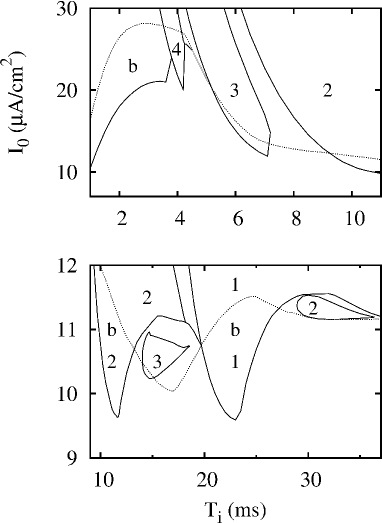
Figure 1: Response diagram in the noiseless case for stimulation by rectangular current pulses of width $\tau=0.6\textrm{ms}$ and height $I_{0}$. The top (bottom) panel shows the high (intermediate) frequency regime. Bistable regions are marked ”b”. Some smaller bistable areas remain unlabeled. They are limited by a dotted line from above and a solid line from below. Labels 1,2,3, and 4 mark regions with 1:1,2:1,3:1, and 4:1 mode locking, respectively. The resonance area near $T_{i}=17\textrm{ms}$ is dominated by the 3:1 state and higher order states. The second resonance near $T_{i}=34\textrm{ms}$ is dominated by the 2:1 mode. Higher modes appear near the threshold at $T_{i}\simeq 34\textrm{ms}$.

Figure 1 shows the response diagram in the $T_{i}-I_{0}$ plane without noise, where $T_{i}$ is the stimulus period. The main resonance is located at $T_{i}\simeq 17\textrm{ms}$. The second order resonance is present at $T_{i}\simeq 34\textrm{ms}$ and the third one at $T_{i}\simeq 51\textrm{ms}$ (not shown). The dotted line separates the region with a single solution from the area where two solutions coexist. Bistable solutions appear between the resonant regions near $T_{i}=11\textrm{ms}$ and $T_{i}=23\textrm{ms}$. In these regimes the transition to excitability occurs via the subcritical Hopf bifurcation. The picture is more complicated at the frequencies above 250 Hz, where the quiescent state often coexists not with a limit cycle but with a set of irregular orbits. The boundaries of bistable regions are determined with a simple continuation algorithm. The initial conditions of each run with a new value of a bifurcation parameter are equal to the end values from the previous iteration.

The firing rate $f_{o}/f_{i}$ depends continuously on $I_{0}$ between the tip of the resonance at $T_{i}\simeq 17\textrm{ms}$ and the bistable area, which begins at $T_{i}\simeq 20\textrm{ms}$. Here $f_{o}$, $f_{i}$ is output, input frequency, respectively. For $14\textrm{ms}<T_{i}<17\textrm{ms}$ bistable intervals with integer $p/q$ ratio alternate with irregular response, whose long-time average is a continuous function of $I_{0}$ and $T_{i}$. Earlier, Clay reported Clay (2003) an irregular graded response near the excitation edge within a revised HH model Clay (1998) stimulated by 1-ms rectangular current pulses and trains of half-sine waves. This variability was attributed to the deterministic nonlinear dynamics of the model.

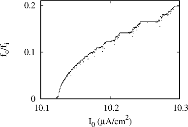
Figure 2: The firing rate as a function of the current pulse height at the resonance $T_{i}=17.5\textrm{ms}$. Here $\tau=0.6\textrm{ms}$. Near the firing threshold $f_{o}$ is approximately a square root function of the pulse amplitude. Further away from the threshold the dependence of $f_{o}$ on $I_{0}$ between the mode-locked states is irregular and nonmonotonic.

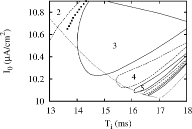
Figure 3: Details of the response diagram at the resonance. Borders of even (odd) mode-locked states are shown with broken (continuous) lines respectively. The dotted lines mark the transitions to repetitive firing. Areas enclosed by the dotted line and continuous or broken lines are bistable. Numbers 2,…,5 indicate the states 2:1,…,5:1. The states beyond 7:1 are not shown. Filled squares indicate the parity multimodal transition between even-only and all modes.

For $T_{i}\geq 17\textrm{ms}$ the firing rate is approximately a square root function of the deviation from the threshold current amplitude (see Fig. 2). This dependence is characteristic of a saddle-node bifurcation Strogatz (1994). The scaling $f_{o}/f_{i}\sim(I_{0}-I_{t}h)^{\beta}$, with $\beta=1/2$ is reminiscent of a mean-field second-order phase transition, with $f_{o}/f_{i}$ playing the role of an order parameter. The same exponent is obtained for a relaxation time near $I_{c}\simeq 6.264\mu\textrm{A/cm}^{2}$ for a constant current $I$ Roa et al. (2007), where $I_{c}$ is the value of $I$ at the saddle-node bifurcation. Below $I_{c}$ the neuron returns to quiescence after emitting a series of spikes. The relaxation time, defined as the time from the first to the last spike, diverges as $(I_{c}-I)^{\Delta}$, where $\Delta\simeq 1/2$. Similar values of $\Delta$ were obtained for the Morris-Lecar and FitzHugh-Nagumo models Roa et al. (2007).

Figure 3 shows the bifurcation diagram near the tip of the resonance. The synchronized states alternate with irregular firing. There are small bistable regions where the quiescent state coexists with a limit cycle. We have calculated their boundaries for states up to order 5:1. It is likely that they extend all the way to the tip of the resonance. The behavior in the intermediate regions is chaotic due to a competition between odd and even modes Borkowski (2009a). An example of $V(t)$ dependence for a point located between states 2:1 and 3:1 is shown in Fig. 4. This sample contains only one odd multiple of the input period. Odd interspike intervals vanish in the vicinity of the 2:1 state. Careful analysis of the interspike interval histograms (ISIH) reveals a transition between the set of even and the set of all modes. This parity transition of ISIHs in the HH model could be tested experimentally in a squid axon experiment, similar to the odd-all transition discovered earlier Takahashi et al. (1990); Borkowski (2010b).

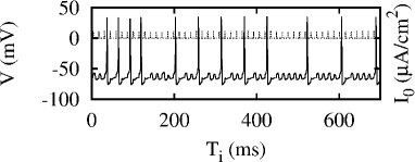
Figure 4: Sample voltage trace in the chaotic regime near the transition between even-only and all modes. The applied current pulses are shown with dotted lines. There is only one odd multiple (7:1) of the input period in this sample. Here $T_{i}=13.9\textrm{ms}$ and $I_{0}=10.75\mu\textrm{A/cm}^{2}$.

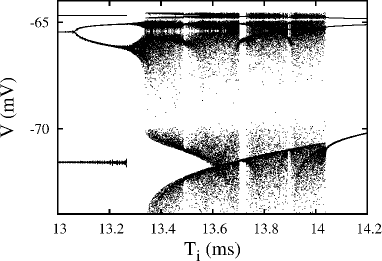
Figure 5: The Poincare section of the membrane potential near the bistable region and irregular regime for current amplitude $I_{0}=10.65\mu\textrm{A/cm}^{2}$. The values of $V(t)$ in each run are recorded at the points $t=nT_{i}$, where $n=1,2,...$. The lowest and the highest flat branches on the left belong to the 2:1 states. The middle one belongs to the steady state. It undergoes a period doubling bifurcation on approach to the irregular regime above $T_{i}=13.3\textrm{ms}$.

The transition between quiescence and chaotic firing marked by the dotted line in the intermediate zones between the locked-in states occurs via period doubling (see Fig. 5). The lowest and the highest values of $V$ below $T_{i}\simeq 13.24\textrm{ms}$ belong to the 2:1 limit cycle. The line slightly below $V=-65\textrm{mV}$, splitting above $T_{i}=13\textrm{ms}$, is associated with the steady state.

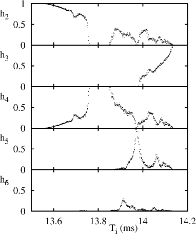
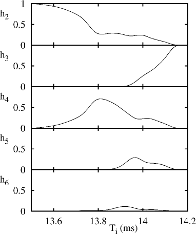
Figure 6: Histograms of the lowest order modes for $D=0$ (left) and $D=10^{-5}$ (right) at $I_{0}=10.75\mu\textrm{A/cm}^{2}$. This is an irregular firing regime between the states 2:1 and 3:1. Data in the noisy case are Bezier-smoothed averages.

The even, odd multiples of $T_{i}$ dominate near the states with even, odd $p/q$ ratio, respectively (see Fig. 6, left). This is a general property of regimes of irregular firing. Starting from the 2:1 mode, the histogram weight is gradually transferred to the 4:1 mode, which dominates for $T_{i}$ slightly below the even-all transition point $T_{ea}$. On the other side of $T_{ea}$, $h_{5}=1$ over a narrow interval.

The histogram of the dominant modes for $D>0$ is shown in Fig. 6 (right). Some weight is now transferred to lower modes. The 4:1 and 5:1 modes are still well pronounced over a range of $T_{i}$ but they are now mixed with 2:1 and 3:1 modes, respectively. Noise extends the range of presence of high order modes around $T_{ea}$, as expected.

The average firing rate between nearby n:1 and $(\textit{n}\textrm{+1):1}$ states often has a narrow local minimum due to the presence of slower modes. The minima are more pronounced near the excitation threshold along the left edge of the resonance tip in Fig. 3, where $T_{i}<17\textrm{ms}$. One such valley is shown in Fig. 7. Here the 4:1 mode dominates in a narrow range of parameter values below the parity transition.

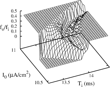
Figure 7: Minimum of the firing rate between the 2:1 and 3:1 states for the noiseless stimulus. The state 4:1 is located near the 2:1 mode.

The firing rate minimum is robust to small levels of noise, as can be seen in Fig. 8. The minimum of $f_{o}$ occurs for $T_{i}\gtrsim T_{ea}$, where modes of both parity are available. In the odd-all transition of the high-frequency regime Borkowski (2009a) the minimum $f_{o}$ was similarly located close to the transition, on the side of all modes.

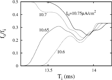
Figure 8: The firing rate as a function of $T_{i}$ in the intermediate region between the 2:1 and 3:1 states for $D=10^{-5}$ and $T_{i}=10.75\textrm{ms}$. The competition of odd and even modes manifests itself as a minimum of the firing rate.

It is well known that the HH neuron has a tendency to spike in bursts when subjected to a noisy stimulus in a bistable regime. If the deterministic system is prepared in one of high order bistable states from Fig. 3, the addition of noise results in slow bursts, where the ISI within a burst is a high integer multiple of $T_{i}$. An example is shown in Fig. 9, where each burst’s ISI is equal to $3T_{i}$. We expect slow bursts of order 6:1 and higher to be found in a more detailed calculation.

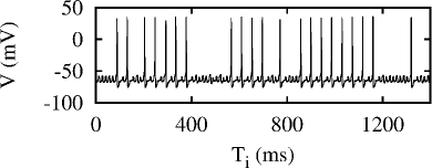
Figure 9: Sample voltage trace in the bistable regime of the state 3:1 under the influence of small noise. The most common form of response consists of 3:1 bursts separated by longer silent intervals. Here $T_{i}=13.9\textrm{ms}$, $I_{0}=10.75\mu\textrm{A/cm}^{2}$, and $D=10^{-3}$.

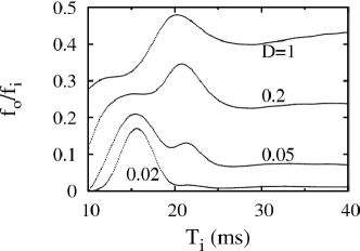
Figure 10: The firing rate as a function of $T_{i}$ for different noise levels and $I=10\mu\textrm{A/cm}^{2}$, about $0.1\mu\textrm{A/cm}^{2}$ below the deterministic threshold.

For stimuli below the deterministic threshold noise activates firing with maximum response at the resonant frequency (see Fig. 10). When noise is larger, excitations into the 2:1 state occur more frequently and the maximum of the firing rate shifts toward $T_{i}=20\textrm{ms}$. This maximum is a result of the interplay between the 1:1 mode and the 2:1 mode. The relative frequency of participation of the 2:1 mode grows sharply for intermediate noise levels in the neighborhood of the bistable regime for $T_{i}\simeq 20\textrm{ms}$.

For signals with a periodic subthreshold component noise may play the role of a frequency selector. In a network with some elements firing in unison at the resonant frequency the remaining uncorrelated neurons also play an important role. The intensity of their background activity may select the firing rate of a network.

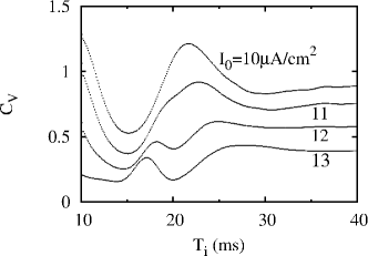
Figure 11: The coefficient of variation as a function of $T_{i}$ for different pulse amplitudes. The noise intensity if fixed at $D=0.2$. The local minimum at larger $I_{0}$ follows the left edge of the 1:1 regime.

The dependence of $C_{V}$ on $T_{i}$ for fixed noise intensity is shown in Fig. 11. As expected, the most coherent response occurs near the resonance. The minimum near $T_{i}=20\textrm{ms}$ for suprathreshold inputs follows the left edge of the 1:1 region from Fig. 1. For stimuli below threshold there is a deep minimum at the resonance and a large maximum in the bistable regime for $T_{i}>20\textrm{ms}$.

For suprathreshold stimulation in the resonance regime the firing rate in general increases monotonically as a function of $D$ with the exception of states having $p/q$ values close to 1 (see Fig. 11). Starting in the 1:1 state at $D=0$, increasing noise slows down the response by annihilating some of the action potential spikes. The minimum $f_{o}/f_{i}$ is reached at an intermediate $D$. In the limit of large noise $f_{o}$ approaches the inverse of the refractory period. The $C_{V}$ maxima are caused by redistribution of histogram weight among several principal modes. This effect was described earlier as stochastic coherence antiresonance Borkowski (2010b). Maximization of spike train incoherence was shown earlier to occur in the FitzHugh-Nagumo Lacasta et al. (2002) and leaky integrate-and-fire Lindner et al. (2002) models. However in those studies the maxima of $C_{V}$ were not accompanied by the minima of $f_{o}/f_{i}$.

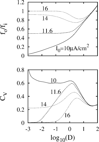
Figure 12: The firing rate and $C_{V}$ as a function of $D$ for several values of $I_{0}$ and $T_{i}=17\textrm{ms}$. Maximum of $C_{V}$ at intermediate values of $D$ is due to the multimodal distribution of interspike intervals.

Figure 13: The response diagram in the presence of noise. Solid lines are the boundaries of the main mode-locked states without noise (see also Fig. 1). The broken and dotted lines are boundaries for $D=10^{-3}$ and $10^{-2}$, respectively.

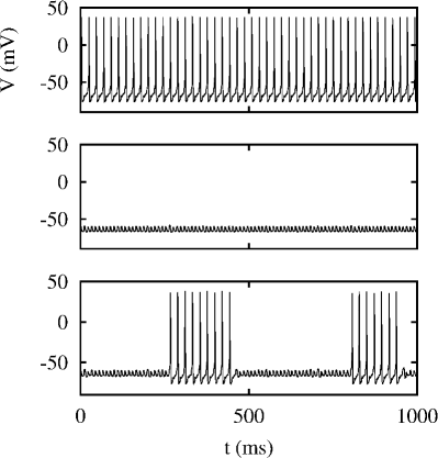
Figure 14: Sample dependence of $V(t)$ for three intensities of noise, from top to bottom: $D=0.001,0.01$, and $0.03$. The spiking action is switched off for intermediate values of $D$. Here $T_{i}=11\textrm{ms}$, $I_{0}=10.5\mu\textrm{A/cm}^{2}$.

Figure 13 shows the response diagram in the presence of noise. The tip of the resonance is broadened and shifted to higher frequencies. The 3:1 state vanishes completely for $D$ slightly larger than $10^{-3}$. Higher-order states are more sensitive to noise and are quickly washed out. The bistable area at the edge of the 2:1 state shrinks more gradually. When bistability is finally eliminated, $f_{o}$ remains discontinuous over part of that border. For $D=10^{-2}$ the discontinuity occurs below $T_{i}\simeq 10.5\textrm{ms}$. Above $T_{i}\simeq 10.5\textrm{ms}$ the firing rate is a continuous function of $I_{0}$. The behavior in the immediate vicinity of $T_{i}=10.5\textrm{ms}$ seems to be weakly irregular. A more detailed study would be needed for a proper description of this area. The loss of stability by the 2:1 state in favor of the quiescent state and further transition to bursting are illustrated in Fig. 14.

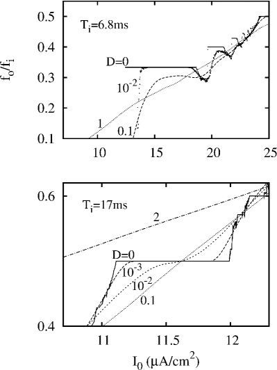
Figure 15: Typical behavior of the average firing rate in the regime of high (top) and moderate frequency (bottom) for different noise levels. At high frequencies and small noise the response is initially slowed down over an entire plateau, starting from both edges. At the lower diagram $f_{o}$ is held steady in the central part of the plateau, decreasing at the left edge and increasing at the right edge. The average firing rate in the central part of the plateau is preserved up to $D\simeq 0.1$. The irregular nonmonotonic behavior in the deterministic case is smoothed out for very small levels of noise.

The reaction to noise at high frequencies is qualitatively different from behavior at near-resonant frequencies (see Fig. 15). In the top panel of Fig. 15 the firing rate drops almost everywhere for small $D$. This is easy to understand if we recall that the odd-all multimodal transition Borkowski (2009a, 2010b) occurs just below $I_{0}=20\mu\textrm{A/cm}^{2}$. The slow modes are easily available in this regime and small perturbations suffice to switch the system among different trajectories. The firing rate drops over the entire 3:1 plateau due to the appearance of the 5:1, 7:1 and other odd modes. For larger $D$ also the even modes are sampled by the system and $f_{o}/f_{i}$ increases.

At moderate, near-resonance frequencies, the central part of the 2:1 plateau in the lower part of Fig. 15 is more robust to noise. The average $f_{o}$ is preserved for $D$ up to $0.1$. Noise induces both the 1:1 mode as well as the 3:1 and slower modes. However the participation rate of the 1:1 mode is balanced by the slower modes in such a way that average $f_{o}/f_{i}$ remains close to 2. This type of resilience to noise, characteristic of the resonance regime, can also be seen in other mode-locked states.

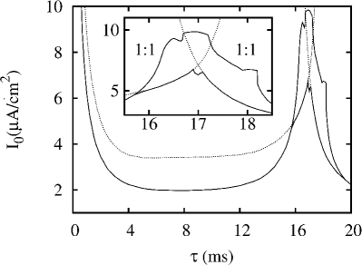
Figure 16: Bifurcation diagram near the excitation threshold as a function of the current pulse width. The input period is set at $T_{i}=17\textrm{ms}$. At $\tau=17\textrm{ms}$ the input current is constant. The details of the antiresonant limit with bistable behavior are shown in the inset. Solid lines mark the excitation threshold. The dotted lines are the boundaries of the 1:1 state.

Finally, let us briefly describe the role played by the current pulse width $\tau$. Figure 16 shows the excitation threshold as a function of $\tau$ for a resonant drive, $T_{i}=17\textrm{ms}$. Initially the threshold decreases as the inverse of $\tau$. For $\tau>8\textrm{ms}$ the tip of the resonance (shown in Fig. 3) gradually becomes narrower and vanishes. The threshold rises again and reaches maximum near $\tau=17\textrm{ms}$, when $I(t)=\textrm{const}$. Bistability appears above $\tau\simeq 16\textrm{ms}$. It is clear that stimulation by a constant current forces the neuron into an antiresonant regime. The bifurcation diagram in Fig. 16 implies that the addition of any charge-unbalanced component to the constant stimulus takes the system away from this antiresonant limit. The precise nature of such a component, whether deterministic or stochastic, is not important. What matters is the amount of charge delivered within approximately $4\textrm{ms}$ from the stimulus onset.

III Conclusions

We studied the response of the HH neuron to a periodic pulse current with a Gaussian noise. The global bifurcation diagram in the $T_{i}-I_{0}$ plane has a rich structure near the excitation threshold, where resonant regimes alternate with antiresonant ones. The model is bistable between the resonances and in the limit of high-frequency stimulation.

The firing rate is a continuous function of $I_{0}$ for $T_{res}\lesssim T_{i}<20\textrm{ms}$. The scaling of the firing rate with $(I_{0}-I_{th})^{1/2}$ is a signature of a saddle-node bifurcation at the threshold. For $T_{i}\lesssim T_{res}$ bistable regions are separated by areas of irregular response with no well defined threshold and approximately continuous dependence of $f_{o}/f_{i}$ on input parameters. As $T_{i}$ approaches $T_{res}$ from below, the subcritical Hopf bifurcation gradually softens. Bistable regions occupy smaller portions of the parameter space and disappear before $T_{i}=T_{res}$. The change of the type of neuronal excitability is important in the context of preventing the so called dynamical diseases, such as epilepsy, Alzheimer’s, and Parkinson’s disease. It was shown in the HH Wang et al. (2007); Xie et al. (2008a) and the Hindmarsh-Rose Xie et al. (2008b) models that this could be obtained by introducing an additional control function. We demonstrated that the threshold behavior can also be altered by selecting the frequency and amplitude of external current.

For subthreshold stimuli noise enables spiking in the vicinity of the resonance. The stimulus frequency, for which the maximum firing rate is obtained, depends on the magnitude of noise. For large $D$, the maximum $f_{o}$ occurs for $T_{i}>T_{res}$. It would be interesting to investigate the same regime in a HH network where the connectivity pattern of neurons as well as their individual properties might lead to the emergence of subpopulations of neurons firing with different average frequencies in response to a correlated input with background noise. It was shown earlier by several authors that both the background noisy activity Ho and Destexhe (2000); Chance et al. (2002) and correlated inputs Stevens and Zador (1998) are important in explaining the neuronal response in vivo. Qualitative results of this work do not depend on the precise functional form of the current pulse provided the width of each pulse does not exceed 4 ms. This invariance of the bifurcation diagram in the $T_{i}-I_{0}$ plane is not surprising because for short pulses the HH neuron’s threshold is determined by the amount of charge delivered per pulse Koch (1999).

We have also found a new even-all multimodal transition occurring between the states 2:1 and 3:1 close to the main resonance. For input period $T_{i}$ below this singularity only even response modes exist. Both even and odd modes appear above the transition. This effect is accompanied by a minimum of the firing rate, located close to the parity transition, on the side of all modes. Similar transitions may exist in other excitable systems.

Our results are also relevant to studies of auditory nerve fiber responses to electric stimulation Matsuoka et al. (2000); Macherey et al. (2007); O’Gorman et al. (2009, 2010). At low stimulation rates auditory nerve fibers fire regularly and are locked in to applied stimulus. At high stimulation rates these fibers respond irregularly. Some researchers attributed this effect to physiological noise Morse and Evans (1996); Moss et al. (1996). However, an analysis within the FitzHugh-Nagumo model showed that the firing irregularities at high frequencies may be caused by deterministic dynamical instability O’Gorman et al. (2009, 2010). We have found similar instabilities in the HH model. They appear at high stimulation frequencies and along the excitation threshold. Both of these regimes are relevant to studies of hearing sensitivity.