Exact sampling for intractable probability distributions via a Bernoulli factory

Abstract

Many applications in the field of statistics require Markov chain Monte Carlo methods. Determining appropriate starting values and run lengths can be both analytically and empirically challenging. A desire to overcome these problems has led to the development of exact, or perfect, sampling algorithms which convert a Markov chain into an algorithm that produces i.i.d. samples from the stationary distribution. Unfortunately, very few of these algorithms have been developed for the distributions that arise in statistical applications, which typically have uncountable support. Here we study an exact sampling algorithm using a geometrically ergodic Markov chain on a general state space. Our work provides a significant reduction to the number of input draws necessary for the Bernoulli factory, which enables exact sampling via a rejection sampling approach. We illustrate the algorithm on a univariate Metropolis-Hastings sampler and a bivariate Gibbs sampler, which provide a proof of concept and insight into hyper-parameter selection. Finally, we illustrate the algorithm on a Bayesian version of the one-way random effects model with data from a styrene exposure study.

and

1 Introduction

Suppose we want to explore a probability distribution $\pi$ defined on $\mathsf{X}$. Further suppose $\pi$ is intractable in the sense that direct (i.i.d.) sampling is unavailable. In this setting, the Markov chain Monte Carlo (MCMC) method can be a useful tool since it is often straightforward to construct and simulate an ergodic Markov chain that has $\pi$ as its stationary distribution (Chen et al.,, 2000; Robert and Casella,, 1999; Liu,, 2001). The two main drawbacks of MCMC relative to direct sampling from $\pi$ are (i) the difficulty in ascertaining how long the Markov chain needs to be run before it gets “close” to $\pi$ (see, e.g., Jones and Hobert,, 2001), and (ii) the difficulty in deriving and calculating asymptotically valid standard errors for the ergodic averages that are used to approximate intractable expectations under $\pi$ (see, e.g., Flegal et al.,, 2008).

A desire to overcome these problems has led to the development of clever techniques using a Markov chain to create an algorithm that produces i.i.d. draws from the stationary distribution (e.g., Craiu and Meng,, 2011; Green and Murdoch, 1999; Huber,, 2004; Propp and Wilson,, 1996; Wilson,, 2000). Unfortunately, very few of these so-called perfect sampling algorithms have been developed for the distributions that arise in realistic statistical applications, which typically have uncountable support. Asmussen et al., (1992) and Blanchet and Meng (2005) provide one such algorithm applicable to Markov chains on general state spaces. The main assumption necessary is that the chain satisfies a one-step minorization condition. As we describe later, under this condition the stationary distribution admits a mixture representation, suggesting the following two-step sampling approach: sample the discrete distribution corresponding to the mixture weights, then sample the selected mixture component.

This approach has never been successfully implemented, however, it has been used to obtain approximate draws from $\pi$, see for example Blanchet and Thomas, (2007), Hobert et al., (2006) and Hobert and Robert, (2004). The difficult part is drawing from the discrete distribution corresponding to the mixture weights, which is done via a rejection sampling approach. In this paper, we provide solutions to a number of practical problems and illustrate the algorithm on three examples. This requires overcoming two challenges: (i) obtaining a dominating proposal distribution and (ii) generating a ${\rm Bernoulli}$ variate to decide whether a proposed draw is accepted or not. While (ii) might seem trivial, the challenge is that we are unable to (exactly) compute the success probability for this ${\rm Bernoulli}$ variate.

A solution to (i) requires identification of a bounding (proposal) probability mass function for the target mass function. Previously, Blanchet and Meng, (2005) proposed an upper bound on moments associated with the target mass function. Blanchet and Thomas, (2007) used output from a preliminary run of the Markov chain to construct an approximate upper bound. We provide an explicit bound for Markov chains satisfying a geometric drift condition using results from Roberts and Tweedie, (1999).

A solution to (ii) will determine whether to accept a proposed draw. The decision is made by generating a ${\rm Bernoulli}$ random variable with success probability that involves the ratio between the target and proposal mass functions. In our case, the target mass function is unknown, apparently making this step impossible. However, one can still generate such a ${\rm Bernoulli}$ variate, using a so-called Bernoulli factory (Keane and O’Brien,, 1994). Briefly, a Bernoulli factory is an algorithm that outputs a ${\rm Bernoulli}$ variate with success probability $f(p)$, from i.i.d. ${\rm Bernoulli}(p)$ variates, when $f$ is known but $p$ is unknown.

The rejection sampling approach requires a Bernoulli factory algorithm for $f(p)=ap$ and $a\in(1,\infty)$. Nacu and Peres, (2005) and Latuszynski et al., (2011) provide an algorithm when $a=2$, but their algorithms are computationally demanding and scale poorly for $a\in(1,\infty)$. For example when $p\in(0,.4)$, one requires at least $65,536$ ${\rm Bernoulli}(p)$ random variables to generate one ${\rm Bernoulli}(2p)$ variate. In this paper, we provide an algorithm for any $a\in(1,\infty)$ that reduces the computational time substantially. For example when $p\in(0,.4)$, we can obtain a ${\rm Bernoulli}(2p)$ variate with only $256$ ${\rm Bernoulli}(p)$ random variables. This is an important reduction because the Bernoulli factory accounts for much of the computational time in the exact sampling algorithm. Section 3 contains a full description the Bernoulli factory and our modification.

Our solutions to (i) and (ii) yield an exact sampling algorithm for $\pi$. The algorithm is suitable even for intractable distributions on general state spaces: that is, for distributions that typically arise in statistical applications. This is an important extension, since very few existing algorithms apply to general state spaces, but it is limited in the sense that one must be able to establish a drift and associated minorization condition for the underlying Markov chain. The current algorithm can be computationally demanding, however we have successfully implemented it in three examples.

Our first example considers a univariate Metropolis-Hastings sampler for which we obtain 1000 i.i.d. draws. The second example considers a slightly more complicated bivariate Gibbs sampler where we again obtain 1000 i.i.d. draws. These two examples could be considered toy examples in the sense that i.i.d. observations are available for each. However, they provide insights into the performance and hyper-parameter selection of the algorithm.

Our final example considers a Bayesian version of the classical one-way random effects model that is widely used to analyze data. We illustrate the exact sampling algorithm, using data from a styrene exposure study, to obtain 20 i.i.d. draws. This is the first successful implementation of an exact sampling algorithm for a model of this type. Our analysis considers a balanced design and requires development of a suitable drift condition, which improves upon the existing drift constants of Tan and Hobert, (2009).

These examples give hope for exact sampling algorithms for general state space Markov chains in more complicated settings. Even if we are unable to obtain multiple draws in these settings, a single exact draw will alleviate the need for burn-in entirely.

The rest of this paper is organized as follows. Section 2 provides the mixture representation of $\pi$, details the rejection sampling approach and bounds the tail probabilities of the proposal distribution. Section 3 introduces the Bernoulli factory and proposes a new target function that speeds up the algorithm significantly. Section 4 gives the full exact sampling algorithm. Sections 5 and 6 implement the algorithm for two toy examples and a Bayesian version of a one-way random effects model, respectively. Finally, Section 7 discusses our implementation and provides some general recommendations to practitioners.

2 Exact sampling via a mixture distribution

Suppose we want to explore the intractable probability measure $\pi(dx)$ defined on the measurable space $\left(\mathsf{X},{\cal B}(\mathsf{X})\right)$. Let $P:\mathsf{X}\times{\cal B}(\mathsf{X})\rightarrow[0,1]$ be a Markov transition function and let $X=\{X_{n}\}_{n=0}^{\infty}$ denote the corresponding Markov chain. Then for $x\in\mathsf{X}$ and a measurable set $A$,

$$P(x,A)=\Pr\left(X_{n+1}\in A|X_{n}=x\right)\;.$$

Assume that $\pi$ is an invariant measure for the chain; i.e., $\pi(A)=\int_{\mathsf{X}}P(x,A)\,\pi(dx)$ for all measurable $A$. Assume further that $X$ satisfies the usual regularity conditions, which are irreducibility, aperiodicity and positive Harris recurrence. For definitions, see Meyn and Tweedie, (1993) and Roberts and Rosenthal, (2004). Finally, assume we are able to simulate the chain; that is, given $X_{n}=x$, we have the ability to draw from $P(x,\cdot)$.

The exact sampling algorithm considered here utilizes a mixture representation for $\pi$ (Hobert et al.,, 2006; Asmussen et al.,, 1992; Hobert and Robert,, 2004), however, we must first develop the split chain. The main assumption necessary is that $X$ satisfies a one-step minorization condition, i.e. there exists a function $s:\mathsf{X}\rightarrow[0,1]$ satisfying $\int_{\mathsf{X}}s(x)\,\pi(dx)>0$ and some probability measure $Q(dy)$ on $(\mathsf{X},{\cal B}(\mathsf{X}))$ such that,

$$P(x,A)\geq s(x)\,Q(A)\;\;\mbox{for all}\;x\in\mathsf{X}\;\mbox{and}\;A\in{\cal B}(\mathsf{X})\;.$$ (1)

Given $X$ satisfies the one-step minorization condition at (1), then $P$ can be decomposed as

$$P(x,dy)=s(x)\,Q(dy)+\left(1-s(x)\right)\,R(x,dy)\;,$$ (2)

where

$$R(x,dy)=\frac{P(x,dy)-s(x)\,Q(dy)}{1-s(x)}\;,$$

and define $R(x,dy)=0$ if $s(x)=1$. It is helpful to think of (2) as a mixture of two Markov transition functions with probabilities $s(x)$ and $1-s(x)$. Equation (2) shows that it is possible to simulate $X_{n+1}$ given $X_{n}=x$ as follows: Flip a coin (independently) that comes up heads with probability $s(x)$. If the coin is a head, take $X_{n+1}\sim Q(\cdot)$; if it’s a tail, take $X_{n+1}\sim R(x,\cdot)$.

This decomposition has several important applications in MCMC. Indeed, it can be used to perform regenerative simulation (Hobert et al.,, 2002; Mykland et al., 1995) and to derive computable bounds on the convergence rate of $X$ (Rosenthal,, 2002, 1995; Lund and Tweedie,, 1996; Roberts and Tweedie,, 1999).

Now consider a new Markov chain that actually includes the coin flips mentioned above. Let $X^{\prime}=\{(X_{n},\delta_{n})\}_{n=0}^{\infty}$ be a Markov chain with state space $\mathsf{X}\times\{0,1\}$. If the current state is $(X_{n},\delta_{n})=(x,\delta)$, then the next state, $(X_{n+1},\delta_{n+1})$, is drawn as follows. If $\delta=1$, then $X_{n+1}\sim Q(\cdot)$; while if $\delta=0$, $X_{n+1}\sim R(x,\cdot)$. Then, conditional on $X_{n+1}=x^{\prime}$, $\delta_{n+1}\sim\mbox{Bernoulli}(s(x^{\prime}))$. This chain is called the split chain. Equation (2) implies that, marginally, the sequence of $X_{n}$ values in the split chain has the same overall probability law as the original Markov chain $X$ (Nummelin,, 1984, Chapter 4). Note that, if $\delta_{n}=1$, then the distribution of $(X_{n+1},\delta_{n+1})$ does not depend on $x$.

Remark 1.

We can avoid drawing from $Q(\cdot)$ entirely by changing the order slightly. Given $x$ is the current state, we can simply generate $X_{i+1}\sim P(x,\cdot)$ in the usual manner and then generate $\delta_{i}|X_{i},X_{i+1}$ with

$$Pr\left(\delta_{i}=1|X_{i},X_{i+1}\right)=\frac{s(X_{i})q(X_{i+1})}{k(X_{i+1}|X_{i})}\;,$$ (3)

where $q(\cdot)$ and $k(\cdot|x)$ are the densities corresponding to $Q(\cdot)$ and $P$ (Nummelin,, 1984, p. 62).

2.1 A mixture representation of $\pi$

The reason for introducing the split chain is that it possesses an accessible atom, $\mathsf{X}\times\{1\}$. Indeed, each time the set $\mathsf{X}\times\{1\}$ is entered, the split chain stochastically restarts itself (because the next $X_{n}$ has distribution $Q$). Let $\mathbb{N}=\{1,2,3,\dots\}$ and $(X_{0},\delta_{0})\in\mathsf{X}\times\{1\}$, then define the first return time to the atom as

$$\tau=\min\big{\{}n\in\mathbb{N}:(X_{n},\delta_{n})\in\mathsf{X}\times\{1\}\big{\}}\;.$$

Our assumptions about $P$ imply that $\mbox{E}(\tau)<\infty$ and hence the sequence $\{p_{n}\}_{n=1}^{\infty}$ defined by

$$p_{n}=\frac{\Pr(\tau\geq n)}{\mbox{E}(\tau)}$$

is nonnegative, nonincreasing, and sums to one. Let $T$ denote a discrete random variable on $\mathbb{N}$ with $\Pr(T=n)=p_{n}$; also let $Q_{n}$ be the conditional distribution of $X_{n}$ given that the split chain does not return to the atom before time $n$. Thus for any $n\in\mathbb{N}$ and any measurable $A$, $Q_{n}(A)=\mbox{Pr}(X_{n}\in A\mid\tau\geq n)$. (Note that $Q_{1}\equiv Q$.) Then $\pi$ can be written as the following mixture of the $Q_{n}$ values:

$$\pi(dx)=\sum_{n=1}^{\infty}p_{n}\,Q_{n}(dx)\;.$$ (4)

Remark 2.

The representation at (4) can be obtained from results in Asmussen et al. (1992) by applying their methods to the split chain. Alternatively, Hobert and Robert, (2004) obtain the representation when $s(x)$ has the specific form $\varepsilon I_{C}(x)$ and Hobert et al., (2006) obtain the representation with the more general minorization shown here.

The representation at (4) offers an alternative sampling scheme for $\pi$. First, make a random draw from the set $\left\{Q_{1},Q_{2},Q_{3},\dots\right\}$ according to the probabilities $p_{1},p_{2},p_{3},\dots$ and then make an independent random draw from the chosen $Q_{n}$.

Sampling algorithm for $\pi$:

1. Draw $T$ such that $Pr(T=n)=p_{n}$ for $n=1,2,3,\dots$, call the result $t$.

2. Make a draw from $Q_{t}(\cdot)$.

Drawing from $Q_{n}$ is simple even when $n\geq 2$. Indeed, just repeatedly simulate $n$ iterations of the split chain, and accept $X_{n}$ the first time that $\delta_{1}=\cdots=\delta_{n-1}=0$. The challenging part of this recipe is drawing from the set $\left\{Q_{1},Q_{2},Q_{3},\dots\right\}$, i.e. simulating a random variable $T$, since the $p_{n}$ values are not computable. Hobert et al., (2006) and Hobert and Robert, (2004) approximate the $p_{n}$ values, which yields approximate draws from $T$ and thus $\pi$. In this paper, we obtain exact draws from $T$ that result in exact draws from $\pi$.

Remark 3.

Let $K|T=n$ be the number of simulations of the split chain before we get a draw from $Q_{n}$, conditional on $T=n$ from Step 1 above. Then $K|T=n$ is geometric with mean $\mbox{E}(K|T=n)=1/P(\tau\geq n)$. Unfortunately, Blanchet and Meng, (2005) show $\mbox{E}(K)=\infty$, and justifiably argue (4) should not be used for multiple replications. This presents a major challenge in the applicability of our algorithm and others that can be similarly expressed, some of which are discussed in the next section.

2.2 Rejection sampler for $T$

There is one case where simulating $T$ is simple (Hobert et al.,, 2006; Hobert and Robert, 2004). Suppose that in the minorization condition (1), $s(x)\equiv\varepsilon>0$ for all $x\in\mathsf{X}$ (implying the Markov chain is uniformly ergodic) and consider the procedure for simulating the split chain with this constant $s$. In particular, note that the coin flip determining whether $\delta_{n}$ is 0 or 1 does not depend on $x$, and it follows that the number of steps until the first return to the accessible atom has a geometric distribution. Indeed, $\Pr(\tau\geq n)=(1-\varepsilon)^{n-1}$. Hence, $\mbox{E}(\tau)=1/\varepsilon$ and

$$p_{n}=\Pr(T=n)=\frac{\Pr(\tau\geq n)}{\mbox{E}(\tau)}=\varepsilon(1-\varepsilon)^{n-1}\;,$$

so $T$ also has a geometric distribution. Therefore it is easy to make exact draws from $\pi$.

Hobert and Robert, (2004) show this exact sampling algorithm is equivalent to Murdoch and Green,’s (1998) Multigamma Coupler and to Wilson,’s (2000) Read-Once algorithm. It is interesting that (4) can be used to reconstruct perfect sampling algorithms based on coupling from the past despite the fact that its derivation involves no backward simulation arguments. Of course, this exact sampling algorithm will be useless from a practical standpoint if $\varepsilon$ is too small.

Unfortunately, in statistical inference problems, the MCMC algorithms are usually driven by Markov chains that are not uniformly ergodic and, hence, cannot satisfy (1) with a constant $s$. Moreover, there is no efficient method to simulate $T$ where $s$ is non-constant. (When $s$ is non-constant, the distribution of $\tau$ is complex and its mass function is not available in closed form. Hence, the mass function of $T$ is also unknown, which precludes direct simulation of $T$.) Therefore we must resort to indirect methods of simulating $T$.

Fortunately, simulating $\tau$ is trivial—indeed, one can simply run the split chain and count the number of steps until it returns to $\mathsf{X}\times\{1\}$. Because this provides an unlimited supply of i.i.d. copies of $\tau$, we can use a rejection sampling approach (Asmussen et al.,, 1992; Blanchet and Meng,, 2005) to simulate $T$ from the i.i.d. sequence $\tau_{1},\tau_{2},\dots$ (where $\tau_{1}\stackrel{{\scriptstyle d}}{{=}}\tau$).

Suppose there exists a function $d:\mathbb{N}\rightarrow[0,1]$ such that $\sum_{n=1}^{\infty}d(n)=D<\infty$ and $P(\tau\geq n)\leq Md(n)$ where $M$ is a finite, positive constant. Consider a rejection sampler with candidate mass function $d(\cdot)/D$. Thus

$$\frac{\Pr(T=n)}{d(n)/D}=\frac{\Pr(\tau\geq n)/\mbox{E}(\tau)}{d(n)/D}=\frac{D}{\mbox{E}(\tau)}\frac{\Pr(\tau\geq n)}{d(n)}\leq\frac{D}{\mbox{E}(\tau)}M\;,$$

which justifies the following rejection sampler.

Rejection sampler for simulating $T$:

1. Draw $T\sim\frac{d(\cdot)}{D}$. Call the result $n$ and let $a=1/\left[Md(n)\right]$.

2. Draw an independent Bernoulli random variable, $B$, with success probability $a\Pr(\tau\geq n)$. If $B=1$, accept $T=n$; if $B=0$, return to Step 1.

Unfortunately, the standard method of simulating $B$ (by computing $a\Pr(\tau\geq n)$ and comparing it to an independent $\mbox{Uniform}(0,1)$ random variable) is not available to us because the mass function of $\tau$ is unavailable in closed form. However, we may draw $B$ without knowing the value of $\Pr(\tau\geq n)$ using a supply of i.i.d. copies of $\tau$. This is the basis of our exact sampling approach.

Suppose $a\in(0,1]$ and let $p=\Pr(\tau\geq n)$, then there exists a simple solution to generate $B\sim{\rm Bernoulli}(ap)$, which Fill, (1998) calls “engineering a coin flip”. Indeed simulate a single $\tau$ and define

$$W=\begin{cases}1\quad&\text{if }\tau\geq n\\ 0\quad&\text{if }\tau<n\end{cases}\;,$$

hence $W\sim\mbox{Bernoulli}(p)$. If we independently simulate $V\sim\mbox{Bernoulli}(a)$ as usual and set $B=VW$, then

$$\Pr\left(B=1\right)=\Pr\left([V=1]\cap[W=1]\right)=\Pr\left(V=1\right)\Pr\left(W=1\right)=ap\;.$$

That is, $B\sim{\rm Bernoulli}(ap)$, obtained by simulating a single $\tau$ and a single Bernoulli $V$.

When $a\in(1,\infty)$, we will obtain $B\sim{\rm Bernoulli}(ap)$ via the Bernoulli factory described in Section 3. For now assume such a simulation is possible, then what remains to establish is a computable tail probability bound, i.e. the sequence $d(n)$ and the constant $M$.

2.3 Tail probability bound

Blanchet and Meng, (2005) bound the moments of $\tau$, however they do not explicitly determine computable values $M$ and $d(n)$. Fortunately, $\Pr(\tau\geq n)$ can be bounded above by a known constant times a known geometric mass function if $X$ satisfies a geometric drift and associated one-step minorization conditions. We will say a drift condition holds if there exists some function $V:\mathsf{X}\mapsto[1,\infty)$, some $0<\lambda<1$ and some $b<\infty$, such that

$$E\left[V(X_{i+1})|X_{i}=x\right]\leq\lambda V(x)+I_{\left(x\in C\right)}b\quad\text{for all }x\in\mathsf{X}\;.$$ (5)

In addition, we require the associated one-step minorization condition as follows; assume that $s(x)$ is bounded below by $\varepsilon$ on $C$ and that

$$\Pr(x,A)\geq\varepsilon Q(A)\quad\mbox{ for all }x\in C,\ \ A\in{\cal B}(\mathsf{X})\;.$$ (6)

Hobert and Robert, (2004) provide the following bound on $\Pr(\tau\geq n)$ based results in Roberts and Tweedie, (1999). Define $A=\sup_{x\in C}E\left[V(X_{i+1})|X_{i}=x\right]$, $J=(A-\varepsilon)/\lambda$, and

$$\beta^{*}=\begin{cases}\lambda^{-1}&\text{ if }J<1\;,\\ \displaystyle\exp\left\{\frac{\log\lambda\log(1-\varepsilon)}{\log J-\log(1-\varepsilon)}\right\}\leq\lambda^{-1}&\text{ if }J\geq 1\;.\end{cases}$$

Then letting $\phi(\beta)=\log\beta/\log\lambda^{-1}$, if $\beta\in(1,\beta^{*})$, we have

$$\Pr(\tau\geq n) \leq\beta\left[\frac{b}{\varepsilon(1-\lambda)}\right]^{\phi(\beta)}\left[\frac{1-\beta(1-\varepsilon)}{1-(1-\varepsilon)\left(J/(1-\varepsilon)\right)^{\phi(\beta)}}\right]\beta^{-n}$$ (7)

$$=Md(n)\;,$$

where $d(n)=\beta^{-n}$ and

$$M=\beta\left[\frac{b}{\varepsilon(1-\lambda)}\right]^{\phi(\beta)}\left[\frac{1-\beta(1-\varepsilon)}{1-(1-\varepsilon)\left(J/(1-\varepsilon)\right)^{\phi(\beta)}}\right]\;.$$

Note $\sum_{n=1}^{\infty}d(n)=\sum_{n=1}^{\infty}\beta^{-n}=\frac{1}{\beta-1}=D<\infty$ since $\beta\in(1,\beta^{*})$. Having established the inequality in (7), we next detail how to generate $B\sim{\rm Bernoulli}(ap)$ when $a>1$.

3 Bernoulli factory

Given a sequence $W=\{W_{n}\}_{n\geq 1}$ of i.i.d. ${\rm Bernoulli}(p)$ random variables, where $p$ is unknown, a Bernoulli factory is an algorithm that simulates a random variable $B\sim{\rm Bernoulli}(f(p))$, where $f$ is a known function. For the exact sampling algorithm, we require a Bernoulli factory where $f(p)=ap$. This idea arrose in Asmussen et al., (1992) when proposing an exact sampling algorithm for general regenerative processes.

Consider $f:S\mapsto[0,1]$, where $S\subset(0,1)$. Keane and O’Brien, (1994) show is it possible to simulate a random variable $B\sim{\rm Bernoulli}(f(p))$ for all $p\in S$ if and only if $f$ is constant, or $f$ is continuous and satisfies, for some $n\geq 1$,

$$\min\{f(p),1-f(p)\}\geq\min\{p,1-p\}^{n}\quad\forall p\in S\;.$$ (8)

While Keane and O’Brien, (1994) develop the necessary and sufficient conditions on $f$, they do not provide a detailed description of an algorithm. Nacu and Peres, (2005) suggest a constructive algorithm via Bernstein polynomials for fast simulation, i.e. the number of input ${\rm Bernoulli}(p)$ variates needed for the algorithm has exponentially bounded tails. However, we find no practical implementation since it requires dealing with sets of exponential size. Our approach is based on the recent work of Latuszynski et al., (2011), which avoids keeping track of large sets by introducing a single auxiliary random variable.

The general approach, in the formulation of Latuszynski et al., (2011), is to construct two random approximations to $f(p)$, denoted $U_{n}$ and $L_{n}$, which depend on $W_{1},W_{2},\ldots,W_{n}$ and satisfy

$$1\geq U_{n}=U_{n}(W_{1},\dots,W_{n})\>\geq U_{n+1}\geq L_{n+1}\geq L_{n}=L_{n}(W_{1},\dots,W_{n})\geq 0\>\mbox{ a.s. }$$ (9)

The random variables $U_{n}$ and $L_{n}$ approximate $f(p)$ in the sense that $E(U_{n})\searrow f(p)$ and $E(L_{n})\nearrow f(p)$ as $n\rightarrow\infty$. The decision to continue sampling or output a zero or a one in the Bernoulli factory is made using an auxiliary ${\rm Uniform}(0,1)$ variable.

Remark 4.

The almost sure monotonicity requirement in (9) is typically difficult to attain and thus Latuszynski et al., (2011) relax it by using super/submartingales instead.

3.1 Modified target function

For the rejection sampling approach to simulating $T$, we have the ability to simulate $W$ by setting $W_{i}=I(\tau_{i}\geq n)$ for $i\geq 1$. We require a single $B\sim{\rm Bernoulli}(ap)$, where $a=1/[Md(n)]$ is a known constant such that $a>0$. The outcome $B$ determines if we accept or reject the proposed value. For $a\in(0,1]$ we use the simple solution in Section 2 and for $a\in(1,\infty)$ we use the Bernoulli factory.

Unfortunately, the function $f(p)=ap$ on $(0,1/a)$ does not satisfy (8) and cannot be simulated via the Bernoulli factory. However, when restricted to $f(p)=\min\{ap,1-\omega\}$ for $\omega>0$, such a simulation is possible.

Nacu and Peres, (2005) and Latuszynski et al., (2011) provide a detailed algorithm for $a=2$ and $0<\omega<1/4$. Their construction requires a minimum of 65,536 input variables (see Table 1) before the requirement $U_{n}\leq 1$ at (9) is met. This is due to the fact that $f(p)=\min\{2p,1-\omega\}$ is not differentiable and the Bernstein polynomials can approximate general Lipschitz functions at a rate of $1/\sqrt{n}$ (see part (i) of Lemma 6 from Nacu and Peres,, 2005). However, when the target function $f$ is twice differentiable, the rate increases to $1/n$ (see part (ii) of the same Lemma).

This suggests the number of ${\rm Bernoulli}(p)$ input variates required may decrease significantly by using a twice differentiable $f$. With this in mind, we propose extending $ap$ smoothly from $\left[0,\frac{1-\omega}{a}\right]$ to $[0,1]$. Fix $\delta<\omega$ and consider the following function

$$F:\left[0,1-\frac{1-\omega}{a}\right]\rightarrow[0,\delta)\quad\quad F(p)=\delta\int_{0}^{ap/\delta}e^{-t^{2}}dt\;,$$

which is bounded by $\delta$ and twice differentiable, with $F^{\prime}(p)=a\exp\{-a^{2}p^{2}/\delta^{2}\}$ and $F^{\prime\prime}(p)=-2p\frac{a^{3}}{\delta^{2}}\exp\{-a^{2}p^{2}/\delta^{2}\}\leq 0$. Standard calculus also gives $|F^{\prime\prime}(p)|\leq a^{2}\frac{\sqrt{2}}{\delta\sqrt{e}}$. ($F$ is related to the Gauss error function ($\rm erf$), though it can be simply calculated from a standard normal distribution function.)

Then define our target function $f$ as

$$f(p)=\begin{cases}ap&\displaystyle\mbox{ if }p\in\left[0,\frac{1-\omega}{a}\right)\\[9.0pt] \displaystyle(1-\omega)+F\left(p-\frac{1-\omega}{a}\right)&\displaystyle\mbox{ if }p\in\left[\frac{1-\omega}{a},1\right]\end{cases}\;.$$ (10)

In other words, we have extended $ap$ such that $f$ defined at (10) is twice differentiable with $|f^{\prime\prime}|\leq C\equiv a^{2}\frac{\sqrt{2}}{\delta\sqrt{e}}$. Define $a(n,k)=f(k/n)$ and $b(n,k)=a(n,k)+C/(2n)$ using $f$ at (10), then we can state Algorithm 4 of Latuszynski et al., (2011) with our modification.

Algorithm I.

1. Simulate $G_{0}\sim{\rm Uniform}(0,1)$.

2. Compute $m=\min\{m\in\mbox{\msbm N}:b(2^{m},2^{m})\leq 1\}$. Set $n=2^{m}$, $\tilde{L}_{\frac{n}{2}}=0$ and $\tilde{U}_{\frac{n}{2}}=1$.

3. Compute $H_{n}=\sum_{i=1}^{n}W_{i}$, $L_{n}=a(n,H_{n})$ and $U_{n}=b(n,H_{n})$.

4. Compute

   $$L_{n}^{*}=\sum_{i=0}^{H_{n}}\frac{\displaystyle{n-\frac{n}{2}\choose H_{n}-i}{\frac{n}{2}\choose i}}{\displaystyle{n\choose H_{n}}}a\left(\frac{n}{2},i\right)\text{ and }U_{n}^{*}=\sum_{i=0}^{H_{n}}\frac{\displaystyle{n-\frac{n}{2}\choose H_{n}-i}{\frac{n}{2}\choose i}}{\displaystyle{n\choose H_{n}}}b\left(\frac{n}{2},i\right)\;.$$

5. Compute

   $$\tilde{L}_{n}=\tilde{L}_{\frac{n}{2}}+\frac{L_{n}-L_{n}^{*}}{U_{n}^{*}-L_{n}^{*}}\left(\tilde{U}_{\frac{n}{2}}-\tilde{L}_{\frac{n}{2}}\right)\text{ and }\tilde{U}_{n}=\tilde{U}_{\frac{n}{2}}-\frac{U_{n}^{*}-U_{n}}{U_{n}^{*}-L_{n}^{*}}\left(\tilde{U}_{\frac{n}{2}}-\tilde{L}_{\frac{n}{2}}\right)\;.$$

6. If $G_{0}\leq\tilde{L}_{n}$ set $B=1$; if $G_{0}\geq\tilde{U}_{n}$ set $B=0$.

7. If $\tilde{L}_{n}<G_{0}<\tilde{U}_{n}$, set $n=2n$, return to step 3.

8. Output $B$.

Theorem 1.

Suppose $a$, $\delta$ and $\omega$ are constants such that $0<a<\infty$ and $0<\delta<\omega<1$. Further suppose $f(p)$ as defined at (10), $ap\in[0,1-\omega]$ and $W=\{W_{n}\}_{n\geq 1}$ are i.i.d. ${\rm Bernoulli}(p)$. Then Algorithm I outputs $B\sim{\rm Bernoulli}(ap)$. Moreover the probability that it needs $N>n$ iterations equals $a^{2}/n\delta\sqrt{2e}$.

Proof.

See Appendix A. ∎

Remark 5.

Note that the probability Algorithm I needs $N>n$ iterations is independent of the unknown value of $p$. Hence the number of $\mbox{Bernoulli}(p)$ variates required will also be independent of $p$.

Algorithm I provides a constructive algorithm for $a\in(1,\infty)$ and reduces the number of input variables by a factor of over 100, which we demonstrate in the following example. This is a critical improvement since the Bernoulli factory accounts for most of the computational demands of the exact sampling algorithm.

3.2 Bernoulli factory example

Consider generating 10,000 $\mbox{Bernoulli}(ap)$ variates for various values of $a$ while setting $p=0.01$, $\omega=1/5$ and $\delta=1/6$. Table 1 displays the minimum number of $\mbox{Bernoulli}(p)$ variates required, along with the observed mean and standard deviation for the count of $\mbox{Bernoulli}(p)$ variates used to generate 10,000 $\mbox{Bernoulli}(ap)$ variates. We can see for $a=2$ the minimum and observed mean have been reduced substantially when comparing our target function with the Nacu and Peres, (2005) target (N&P). The reduction in observed input$\mbox{Bernoulli}(p)$ variates represents a 120 times reduction in computational time. The N&P implementation always stops the simulation at the minimum, and hence the standard deviation of the count is 0. Table 1 also shows the input variates required increases as $a$ increases. Simulations for other $p$ values (not shown) provide very similar results.

Table 1: Comparison of count of input $\mbox{Bernoulli}(p)$ variates to implement the Bernoulli factory.

a	2 (N&P)	2	5	10	20
Minimum	65536	256	2048	8192	32768
Mean Count	65536	562.9	2439.8	10373	43771
S.D. Count	0	21046	7287.6	54836	3.908e5

4 Exact sampling algorithm

The Bernoulli factory algorithm, Theorem 1, requires $ap<1-\omega$. To this end, let $\kappa>1$ such that $1/\kappa<1-\omega$ and from (7)

$$\Pr(\tau\geq n)\leq Md(n)<Md(n)\kappa\;.$$

Then letting $a=1/\left[Md(n)\kappa\right]$ we have $a\Pr(\tau\geq n)\leq 1/\kappa<1-\omega<1$ for all $n$. The following algorithm results in exact draws from $\pi$.

Exact sampling algorithm for $\pi$:

1. Draw $T^{*}\sim\mbox{Geometric}\left(1-1/\beta\right)$, i.e. $\Pr\left(T^{*}=k\right)=\left(1/\beta\right)^{k-1}\left(1-1/\beta\right)$ for $k=1,2,\dots$, and call the result $n$. Set $a=1/\left[Md(n)\kappa\right]$.

2. If $a\leq 1$, draw a single $\tau$ random variable. Let $W=I(\tau\geq n)$ and independently draw $V\sim\mbox{Bernoulli}\left(a\right)$. Set $B=VW$.

3. If $a>1$, use the Bernoulli factory to obtain $B$, a single Bernoulli random variable with success probability $p=a\Pr(\tau\geq n)$.

4. If $B=1$, accept $T^{*}=n$; if $B=0$, return to Step 1.

5. Make a draw from $Q_{n}(\cdot)$.

The algorithm requires selection of $\varepsilon$, $C$, $\lambda$, and $\kappa$ from a range of possible values (depending on the drift and minorization). Further, $\beta\in(1,\beta^{*})$ must be selected depending on the previously selected parameters. Each selection impacts the algorithm performance and we suggest investigation of different settings for a given example. Our examples in Sections 5 and 6 discuss hyper-parameter selection and provide further recommendations.

5 Toy examples

This section contains two toy examples in the sense that we can obtain i.i.d. samples for each, hence there is no practical reason for considering MCMC algorithms. The purpose is to gain insights into the exact sampler and study its performance.

5.1 Metropolis-Hastings example

This section illustrates the exact sampling algorithm for a Metropolis-Hastings sampler. Suppose that $\mathsf{X}=[0,\infty)$ and $\pi(dx)=f_{X}(x)\;dx$ where $f_{X}(x)=e^{-x}\;I(x\geq 0)$. Consider the function $V(x)=e^{cx}$ for some $c>0$ and suppose we use a Metropolis sampler with a symmetric proposal density $g(\cdot|x)$, which is supported on $[x-\gamma,x+\gamma]$, $\gamma>0$. Then, for $x>\gamma$,

$$E[V(X_{i+1})|X_{i}\,{=}\,x] =\int_{x-\gamma}^{x}V(y)g(y|x)dy+\int_{x}^{x+\gamma}V(y)g(y|x)dy\frac{f(y)}{f(x)}$$

$$+\int_{x}^{x+\gamma}V(x)g(y|x)dy\left(1-\frac{f(y)}{f(x)}\right)$$

$$=\!\int_{x}^{x+\gamma}\!\biggl{(}\!V(2x\,{-}\,y)\,{+}\,V(y)\frac{f(y)}{f(x)}\,{+}\,V(x)\biggl{(}\!1\,{-}\,\frac{f(y)}{f(x)}\!\biggr{)}\!\biggr{)}g(y|x)dy$$

$$=V(x)\int_{x}^{x+\gamma}\!\left(\!e^{-c(y-x)}\,{+}\,e^{(c-1)(y-x)}\,{+}\,1\,{-}\,e^{-(y-x)}\!\right)\!g(y|x)dy.$$

Selecting $g$ to be the uniform density $g(y|x)=\frac{1}{2\gamma}I_{y\in[x-\gamma,x+\gamma]}$, we get

$$E[V(X_{i+1})|X_{i}=x]=V(x)\frac{1}{2\gamma}\int_{0}^{\gamma}\left(e^{-cz}+e^{(c-1)z}+1-e^{-z}\right)dz\>.$$ (11)

When $x\in[0,\gamma]$,

$$E[V(X_{i+1})|X_{i}=x] =\int_{0}^{x}V(y)g(y|x)dy+\int_{x}^{x+\gamma}V(y)g(y|x)dy\frac{f(y)}{f(x)}$$

$$+\int_{x}^{x+\gamma}V(x)g(y|x)dy\left(1-\frac{f(y)}{f(x)}\right)$$

$$=\int_{0}^{x}e^{cy}\frac{1}{2\gamma}dy+\frac{e^{cx}}{2\gamma}\int_{x}^{x+1}e^{(c-1)(y-x)}dy$$

$$+\frac{e^{cx}}{2\gamma}\int_{x}^{x+1}\left(1-e^{-(y-x)}\right)dy\;.$$ (12)

When combined, (11) and (12) obtain a drift condition for the Metropolis-Hastings sampler considered. However, the selection of the constants $c$ and $\gamma$ is crucial to obtaining a reasonable computation time. The constants $\beta$ and $M$, which are described in Section 2.3, also depend on $c$ and $\gamma$. Based on our example in Section 3, our strategy is to maximize $\beta$, which in turn results in small values for $a=1/[Md(n)\kappa]$. Figure 1(a) displays a contour map of $\beta^{*}$ for $c<0.3$ and $\gamma<10$. Based on this plot, we select $c=0.028$ and $\gamma=4$, resulting in $\beta=1.0243$ (as seen below). Evaluating the integrals in (11) and (12) gives the drift condition

$$E[V(X_{i+1})|X_{i}=x]\leq\lambda V(x)+I_{\left(x\in C\right)}b$$

where $\lambda=0.977$, $b=0.1$ and the small set $C=[0,4]$. The interval $[0,\gamma]$ is indeed a small set, since, when $x\in[0,\gamma]$,

$$P(x,dy) \geq g(y|x)dy\min\left\{1,\frac{f(y)}{f(x)}\right\}=\frac{1}{2\gamma}I_{y\in[0,x+\gamma]}dy\min\left\{1,\frac{f(y)}{f(x)}\right\}$$

$$\geq \frac{1}{2\gamma}I_{y\in[0,\gamma]}e^{-y}dy$$

$$= \frac{1-e^{-\gamma}}{2\gamma}\left(\frac{1}{1-e^{-\gamma}}e^{-y}I_{y\in[0,\gamma]}dy\right)\;.$$

This establishes the necessary minorization condition $P(x,dy)\geq s(x)Q(dy)$ where

$$Q(dy)=q(y)dy=\frac{1}{1-e^{-\gamma}}e^{-y}I_{y\in[0,\gamma]}dy\text{ and }s(x)=\frac{1-e^{-\gamma}}{2\gamma}I_{x\in[0,\gamma]}\;.$$

The remaining numerical elements required for the geometric probability bound are: $A=\sup_{x\in C}E[V(X_{i+1}|X_{i}=x])=1.09197$ and $J=(A-\varepsilon)/\lambda=0.99283<1$. Then $\beta=1/\lambda=1.0243$. Finally, the Bernoulli factory hyper-parameters are $\kappa=5/4$ and $\delta=1/6$ resulting in $\omega=0.2$.

Following Mykland et al., (1995), we can now simulate the split chain as follows: (1) draw $X_{n+1}$ from $g(\cdot|X_{n})$ and accept it with probability $\min\bigl{\{}1,\frac{f(X_{n+1})}{f(X_{n})}\bigr{\}}$; (2) if the candidate in step (1) is rejected, set $\delta_{n}=0$, otherwise, generate $\delta_{n}$ as a Bernoulli variate with success probability given by

$$Pr(\delta_{n}=1)=\frac{s(X_{n})q(X_{n+1})}{g(X_{n+1}|X_{n})\min\left\{1,\frac{f(X_{n+1})}{f(X_{n})}\right\}}\;.$$

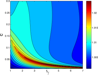
(a) Contour map of $\beta^{*}$.

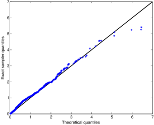
(b) Q-Q plot.

Figure 1: Plots for Metropolis-Hastings example.

Using the exact sampling algorithm, we generated 1000 i.i.d. Exp(1) random variates. Figure 1(b) shows a Q-Q plot of the observed draws versus the theoretical quantiles of the ${\rm Exp}(1)$ distribution. During our simulations none of the proposed $T^{*}$ values which required the use of the Bernoulli factory were accepted. This is due to the fact that our Metropolis-Hastings sampler regenerates very fast, roughly in about 20 moves. Thus for large $T^{*}$, when the Bernoulli factory is necessary, the probability $\Pr(\tau>T^{*})$ is negligible and the Bernoulli factory outputs a zero. Improvements via modified drift and minorization or hyper-parameter selection may improve this situation.

5.2 Gibbs example

Suppose $Y_{i}|\mu,\theta\sim\text{N}(\mu,\theta)$ independently for $i=1,\ldots,m$ where $m\geq 3$ and assume the standard invariant prior $\nu(\mu,\theta)\propto\theta^{-1/2}$. The resulting posterior density is

$$\pi(\mu,\theta|y)\propto\theta^{-(m+1)/2}\exp\left\{-\frac{m}{2\theta}(s^{2}+(\bar{y}-\mu)^{2})\right\}$$ (13)

where $s^{2}$ is the usual biased sample variance. It is easy to see the full conditional densities, $f(\mu|\theta,y)$ and $f(\theta|\mu,y)$, are given by $\mu|\theta,y\sim\text{N}(\bar{y},\theta/m)$ and $\theta|\mu,y\sim\text{IG}((m-1)/2,m\left[s^{2}+(\bar{y}-\mu)^{2}\right]/2)$, hence a Gibbs sampler is appropriate. (We say $W\sim\text{IG}(\alpha,\beta)$ if its density is proportional to $w^{-(\alpha+1)}e^{-\beta/w}I(w>0)$.) We consider the Gibbs sampler that updates $\theta$ then $\mu$; that is, letting $x^{\prime}=(\theta^{\prime},\mu^{\prime})$ denote the current state and $x=(\theta,\mu)$ denote the future state, the transition looks like $(\theta^{\prime},\mu^{\prime})\rightarrow(\theta,\mu^{\prime})\rightarrow(\theta,\mu)$. This Markov chain then has state space $\mathsf{X}=\mathbb{R}^{+}\times\mathbb{R}$ and transition density

$$k(\theta,\mu|\theta^{\prime},\mu^{\prime})=f(\theta|\mu^{\prime},y)f(\mu|\theta,y)\;.$$ (14)

Appendix B provides a drift and minorization condition using a small set in the form

$$C=\left\{(\theta,\mu)\in\mathbb{R}^{+}\times\mathbb{R}:V(\mu,\theta)\leq d\right\}\>,$$

where $V(\theta,\mu)=1+\left(\mu-\bar{y}\right)^{2}$.

Suppose $\bar{y}=1$, $s^{2}=4$, and $m=11$. We set $\lambda=0.5$ and $d=b/(\lambda-(m-3)^{-1})=11/3$ resulting in $\varepsilon=0.5750034$ and $\beta^{*}=1.3958$. Given the allowable range $\beta\in(1,\beta^{*})$, we select $\beta=1.35$, which turns out to be extremely important for implementation. Selection of $\beta$ very close to $\beta^{*}$ or close to 1 seems to cause problems for the Bernoulli factory because of large constant multipliers $a=1/\left[Md(n)\kappa\right]$ given typical proposed $T^{*}=n$ (which depend on $\beta$). Experimentation has shown us values somewhat close to $\beta^{*}$ seem to provide the best results. Finally, the Bernoulli factory hyper-parameters are $\kappa=5/4$ and $\delta=1/6$ resulting in $\omega=0.2$.

Table 2 summarizes the resulting constants given the hyper-parameter choices. Notice the Bernoulli factory will be necessary for proposed values greater than or equal to 10, that is with probability 0.067. The constants for values greater than 20 are not listed. However, these values are of interest since the minimum number of observed $\tau$ values becomes extremely large. While values in this range are uncommon, $P\left(T^{*}>20\right)\approx 0.002$, they occur with enough frequency to slow down the algorithm substantially.

Table 2: Summary constants for Gibbs sampler example with $\beta=1.35$. The row $\min$ refers to the minimum number of observed $\tau$s to implement the Bernoulli factory and $p(n)=P\left(T^{*}=n\right)$.

$n$	1	2	3	4	5	6	7	8	9	10
$p(n)$	0.259	0.192	0.142	0.105	0.078	0.058	0.043	0.032	0.023	0.017
$a$	0.08	0.11	0.14	0.19	0.26	0.35	0.47	0.64	0.86	1.16
$\min$	-	-	-	-	-	-	-	-	-	128
$n$	11	12	13	14	15	16	17	18	19	20
$p(n)$	0.013	0.010	0.007	0.005	0.004	0.003	0.002	0.002	0.001	0.001
$a$	1.57	2.12	2.87	3.87	5.22	7.05	9.52	12.85	17.35	23.42
$\min$	128	256	512	1024	2048	4096	8192	8192	16384	32768

The exact sampling algorithm was used to generate 1000 exact draws from the posterior density at (13). Generating the 1000 draws required approximately 35 hours of computational time, about 2 minutes per draw. A total of 27,665 $T^{*}$ values were proposed of which 69 (0.25%) were greater than 20. Implementing the Bernoulli factory required 1.52e9 $\tau$ values, or 1.52e6 $\tau$ values per exact draw. However, most of the computational time, and necessary $\tau$ values, were used for a small number of proposed $T^{*}$ values. Similar to the Metropolis-Hastings example, none of the accepted $T^{*}$ values were from the Bernoulli factory.

The largest proposed $T^{*}$ value was 37 with $a\approx 3848$ requiring 1.07e9 $\tau$ values (of which 0 were $\geq 37$) to implement the Bernoulli factory. This value alone accounted for about 70% of the total number of $\tau$ values, and hence about 70% of the total computational time. It should be noted that the largest accepted $T^{*}$ value was 9, so proposals unlikely to be accepted account for most of the computational demands. Removing only the largest proposal, the remaining 999 draws required approximately 10 hours of computation, or about 35 seconds per draw.

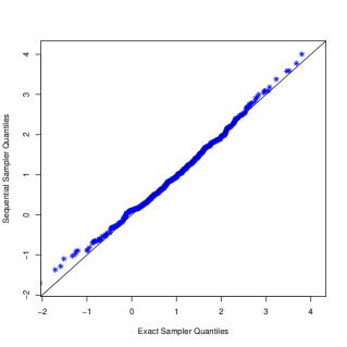
(a) Q-Q plot for $\mu$.

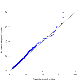
(b) Q-Q plot for $\theta$.

Figure 2: Q-Q plots comparing 1000 exact draws to 1000 i.i.d. draws from a sequential sampler.

Alternatively for this example, we can sequentially sample from (13) to obtain i.i.d. draws (Flegal et al.,, 2008). Figure 2 compares the 1000 exact draws to 1000 i.i.d. draws from a sequential sampler using a Q-Q plot for both $\mu$ and $\theta$. We can see from these plots that the exact sampling algorithm is indeed working well.

6 Bayesian random effects model

This section considers a Bayesian version of the one-way random effects model given by

$$Y_{ij}=\phi_{i}+\zeta_{ij},\quad i=1,\ldots,q,\>j=1,\ldots,m_{i}$$

where the random effects $\phi_{i}$ are i.i.d. $N(\mu,\sigma_{\phi}^{2})$ and independently the errors $\zeta_{ij}$ are i.i.d. $N(0,\sigma_{e}^{2})$. Thus $(\mu,\sigma_{\phi}^{2},\sigma_{e}^{2})$ is the unknown parameter.

Bayesian analysis using this model requires specifying a prior distribution, for which we consider the family of inverse gamma priors

$$\pi(\mu,\sigma_{\phi}^{2},\sigma_{e}^{2})\propto(\sigma_{\phi}^{2})^{-(\alpha_{1}+1)}e^{-\beta_{2}/\sigma_{\phi}^{2}}(\sigma_{e}^{2})^{-(\alpha_{2}+1)}e^{-\beta_{2}/\sigma_{e}^{2}}$$

where $\alpha_{1}$, $\alpha_{2}$, $\beta_{1}$ and $\beta_{2}$ are hyper-parameters. If we let $y=\{y_{ij}\}$ and $\phi=\{\phi_{i}\}$ denote the vectors of observed data and random effects respectively, then the posterior density is as follows

$$\pi\left(\phi,\mu,\sigma_{\phi}^{2},\sigma_{e}^{2}\right)\propto f\left(y|\phi,\mu,\sigma_{\phi}^{2},\sigma_{e}^{2}\right)f\left(\phi|\mu,\sigma_{\phi}^{2},\sigma_{e}^{2}\right)\pi(\mu,\sigma_{\phi}^{2},\sigma_{e}^{2})\;,$$ (15)

where

$$f\left(y|\phi,\mu,\sigma_{\phi}^{2},\sigma_{e}^{2}\right)=\prod_{i=1}^{q}\prod_{j=1}^{m_{i}}\left(2\pi\sigma_{e}^{2}\right)^{-\frac{1}{2}}\exp\left\{-\frac{1}{2\sigma_{e}^{2}}\left(y_{ij}-\phi_{i}\right)^{2}\right\}$$

and

$$f\left(\phi|\mu,\sigma_{\phi}^{2},\sigma_{e}^{2}\right)=\prod_{i=1}^{q}\left(2\pi\sigma_{\phi}^{2}\right)^{-\frac{1}{2}}\exp\left\{-\frac{1}{2\sigma_{\phi}^{2}}\left(\phi_{i}-\mu\right)^{2}\right\}\;.$$

For ease of exposition, we will suppress the dependency on the data $y$ and define the usual summary statistics: $\bar{y}_{i}=m_{i}^{-1}\sum_{j}y_{ij}$, $M=\sum_{i}m_{i}$, $\bar{y}=M^{-1}\sum_{i}\sum_{j}y_{ij}$, $\text{SST}=\sum_{i}m_{i}\left(\bar{y}_{i}-\bar{y}\right)^{2}$ and $\text{SSE}=\sum_{i}\sum_{j}\left(y_{ij}-\bar{y}_{i}\right)^{2}$.

We consider a block Gibbs sampler that updates $\theta=(\sigma_{\phi}^{2},\sigma_{e}^{2})$ then $\xi=(\mu,\phi)$, that is $(\theta^{\prime},\xi^{\prime})\rightarrow(\theta,\xi^{\prime})\rightarrow(\theta,\xi)$. The necessary full conditionals can be obtained via manipulation of (15). That is, $f(\theta|\xi^{\prime})$ is the product of two inverse gammas such that

$$\sigma^{2}_{\phi}|\xi^{\prime}\sim IG\left(\frac{q}{2}+\alpha_{1},\frac{w_{1}(\xi^{\prime})}{2}+\beta_{1}\right)$$

and

$$\sigma^{2}_{e}|\xi^{\prime}\sim IG\left(\frac{M}{2}+\alpha_{2},\frac{w_{2}(\xi^{\prime})+SSE}{2}+\beta_{2}\right)$$

where $w_{1}(\xi)=\sum_{i=1}^{q}(\phi_{i}-\mu)^{2}$ and $w_{2}(\xi)=\sum m_{i}(\phi_{i}-\bar{y}_{i})^{2}$. Further, $f(\xi|\theta)$ is multivariate normal density whose parameters are given in Tan and Hobert, (2009). This Markov chain then has state space $\mathsf{X}=\mathbb{R}^{q+1}\times\mathbb{R}^{2}_{+}$ and transition density

$$k(\xi,\theta|\>\xi^{\prime},\theta^{\prime})=f(\theta|\xi^{\prime})f(\xi|\theta)=f(\sigma_{\phi}^{2}|\xi^{\prime})f(\sigma_{e}^{2}|\xi^{\prime})f(\xi|\theta)\;.$$

Implementation of the exact sampling algorithm requires a drift and associated minorization condition as at (5) and (6). Hobert and Geyer, (1998), Jones and Hobert, (2001, 2004) and Tan and Hobert, (2009) analyze variations of the proposed block Gibbs sampler, however none obtain sufficient constants for a practical implementation of our algorithm. To this end, the following theorem improves upon the drift constants of Tan and Hobert, (2009) for a balanced design while using a simplified version of their drift function.

Theorem 2.

Let $m_{i}=m$ for all $i=1,\dots,q$ and let $\Delta_{2}=1-1/[q(m+1)]+\max\{q(m+1)/m^{2}\>,1/m\}$. Further let $V:\mathbb{R}^{q+1}\times\mathbb{R}^{2}_{+}\rightarrow[1,\infty)$ such that $V(\xi,\theta)=K+\delta_{1}w_{1}(\xi)+\delta_{2}w_{2}(\xi)$ where $K\geq 1$, $\delta_{1}>0$ and $\delta_{2}>0$ and define

$$\lambda^{*}=\max\left\{\frac{1}{q+2\alpha_{1}-2}\>,\frac{\delta_{1}\Delta_{2}/\delta_{2}+q+1}{M+2\alpha_{2}-2}\right\}\;.$$

Then there exists $K\geq 1$, $\delta_{1}>0$ and $\delta_{2}>0$ such that $\lambda^{*}<1$ and (5) holds. That is, for any $\lambda\in(\lambda^{*},1)$,

$$E(V(\xi,\theta)|\xi^{\prime},\theta^{\prime})\leq\lambda V(\xi^{\prime},\theta^{\prime})+b1_{(\xi^{\prime},\theta^{\prime})\in C}$$ (16)

where

$$b =K(1-\lambda)+\frac{2\delta_{1}\beta_{1}}{q+2\alpha_{1}-2}+\frac{(\delta_{1}\Delta_{2}+\delta_{2}(q+1))(SSE+2\beta_{2})}{M+2\alpha_{2}-2}$$

$$+(\delta_{1}+m\delta_{2})\sum_{i=1}^{q}(\bar{y}_{i}-\bar{y})^{2}$$

and

$$C=\{(\xi,\theta)\in\mathbb{R}^{q+1}\times\mathbb{R}_{+}^{2}\>:\>V(\xi,\theta)\leq d\}$$

where $d=b/(\lambda-\lambda^{*})$.

Proof.

See Appendix C. ∎

The drift condition still holds if we increase the small set to

$$C=\{(\xi,\theta)\in\mathbb{R}^{q+1}\times\mathbb{R}_{+}^{2}\>:\>K+\delta_{1}w_{1}(\xi)\leq d,K+\delta_{2}w_{2}(\xi)\leq d\}\;,$$

for which Appendix C provides the associated minorization condition.

6.1 Styrene exposure dataset

We will implement the exact sampling algorithm using the styrene exposure dataset from Lyles et al., (1997) analyzed previously by Jones and Hobert, (2001) and Tan and Hobert, (2009). The data, summarized in Table 3, is from a balanced design such that $m_{i}=m=3$ for $i=1,\ldots,q$, $q=13$, and $M=mq=39$.

Table 3: Styrene exposure data summary statistics.

Worker	1	2	3	4	5	6	7
$\bar{y}_{i}$	3.302	4.587	5.052	5.089	4.498	5.186	4.915
Worker	8	9	10	11	12	13
$\bar{y}_{i}$	4.876	5.262	5.009	5.602	4.336	4.813
	$\bar{y}=4.089,\quad\text{SST}=11.430,\quad\text{SSE}=14.711$

We consider prior hyper-parameter values $\alpha_{1}=\alpha_{2}=0.1$ and $\beta_{1}=\beta_{2}=10$. The drift function at (16) requires specification of drift parameters $K=50$, $\Delta_{2}=6.7585$, $\delta_{1}=1$, and $\delta_{2}=1$ which results in $\lambda^{*}=0.5580$. We then choose $\lambda=0.97$, $b=37.88927$ and $d=91.96992$, resulting in $\varepsilon=0.01269784$.

Table 4: List of 20 i.i.d. $\theta$ draws from the posterior at (15) with the accepted $T^{*}$ values.

Draw	$T^{*}$	$\sigma^{2}_{\phi}$	$\sigma^{2}_{e}$
1	145	2.477	1.2624
2	18	1.234	1.7698
3	286	3.058	1.8791
4	40	2.607	1.2079
5	76	2.177	2.0603
6	287	6.513	1.2870
7	39	5.961	1.5295
8	103	1.642	1.2093
9	194	2.150	1.8129
10	195	2.112	1.4871
11	101	1.101	1.7166
12	2	1.659	1.0805
13	5	5.544	1.2856
14	9	1.505	1.6600
15	1	2.105	1.4137
16	150	2.681	0.7317
17	63	3.131	1.1506
18	64	3.514	1.8245
19	52	2.119	1.1743
20	62	3.571	1.5009

Using these settings $\beta^{*}=1.000092$ and we choose $\beta=1.000083$ resulting in $M=10.19413$. We again used Bernoulli factory hyper-parameters of $\kappa=5/4$ and $\delta=1/6$ resulting in $\omega=0.2$. In this case, the Bernoulli factory is necessary for proposals greater than 30,706, approximately 8% of proposed values. It is extremely likely the output from the Bernoulli factory will be zero since a sample of 1000 i.i.d. $\tau$ values yielded only a maximum of 1278.

The exact sampling algorithm was run until we obtained a 20 i.i.d. draws from the posterior at (15) which took 31,887 proposed $T^{*}$ values and 2.61e8 $\tau$ values for the Bernoulli factory. The accepted $T^{*}$ values and i.i.d. $\theta$ values are listed in Table 4. Notice the maximum accepted $T^{*}$ was 287, which is well below our observed maximum of 1278 from 1000 i.i.d. $\tau$ values. Hence, drawing from $Q_{n}$ was easy and almost all of the simulation time was used for the Bernoulli factory. Obtaining the 20 i.i.d. draws required 24 days of computational time utilizing six processors in parallel (equating to 144 days on a single processor).

7 Discussion

This paper describes an exact sampling algorithm using a geometrically ergodic Markov chain on a general state space. The algorithm is applicable for any Markov chain where one can establish a drift and associated minorization with computable constants. The limitation of the method is that the simulation time may be prohibitive.

Blanchet and Thomas, (2007) implement an approximate version using the Bayesian probit regression example from van Dyk and Meng, (2001) with regeneration settings provided by Roy and Hobert, (2007). This example is ill-suited using the proposed algorithm because of computational limitations related to the Bernoulli factory and in obtaining a practical $\varepsilon$. Specifically, we found (in simpler examples) obtaining a single draw from $\pi$ sometimes required millions of i.i.d. $\tau$ variates. Unfortunately, even using non-constant $s(x)$, the probit example requires about 14,000 Markov chain draws per $\tau$ (Flegal and Jones,, 2010). Hence obtaining a single draw from $\pi$ would require an obscene number of draws from $X$. Implementation for more complicated Markov chains, such as this, likely requires further improvements, or a lot of patience.

Careful analysis of the Markov chain sampler is necessary to find useful drift and minorization constants. Most research establishing drift and minorization is undertaken to prove geometric ergodicity, in which case the obtained constants are of secondary importance. However, performance of the exact sampling algorithm is heavily dependent on these constants. Improving them may be enough to obtain exact samples in many settings.

Alternatively, the speed of the overall algorithm would improve if one could find a bound using non-constant $s(x)$ or a sharper bound with $\varepsilon$. The current bound at (7) could potentially be modified upon by only considering specific models, or specific classes of models.

Finally, one could obtain further improvements to the Bernoulli factory since it requires most of the necessary $\tau$ variates. Our work has already obtained a 100 times reduction in computational time. However there may be further improvements available for the Bernstein polynomial coefficients, modifications to Algorithm 4 of Latuszynski et al., (2011) or an entirely different method to estimate $f$. Hyper-parameter settings also impact performance and could be investigated further.

Appendix A Proof of Theorem 1

Proof.

By construction $f$ is a smooth function $f:[0,1]\rightarrow[0,1-\varepsilon]$ for some $0<\varepsilon<\omega-\delta$. Proposition 3.1 of Latuszynski et al., (2011) and Lemma 6 of Nacu and Peres, (2005) prove existence of an algorithm that simulates $f(p)$ if

• $f$ has second derivative $f^{\prime\prime}$ which is continuous and

• the coefficients $a$ and $b$ satisfy

  $$a(2n,k){2n\choose k} \geq \sum_{i=0}^{k}a(n,i){n\choose i}{n\choose{k-i}}\;,$$ (17)

  $$b(2n,k){2n\choose k} \leq \sum_{i=0}^{k}b(n,i){n\choose i}{n\choose{k-i}}\;.$$ (18)

Condition (i) is clearly satisfied by construction, so it remains to check condition (ii). Since the coefficients $a$ and $b$ are defined through $f$, inequalities (17) and (18) will be checked using the properties of $f$.

Recall $b(n,k)=a(n,k)+C/(2n)$, the inequalities (17) and (18) above can be re-expressed (Nacu and Peres,, 2005) as

$$a(2n,k)\geq E(a(n,X))\text{ and }b(2n,k)\leq E(b(n,X)),$$

where $X$ is a hypergeometric random variable, with parameters $(2n,k,n)$. Using the definition of $a$, and the fact that $f$ is concave, the first inequality is a direct application of Jensen’s inequality. The second part is a straight forward application of Lemma 6 from Nacu and Peres, (2005) and the properties of the hypergeometric distribution.

Finally, the probability the algorithm needs $N>n$ follows directly from definitions of the coefficients $a$ and $b$ and Theorem 2.5 of Latuszynski et al., (2011). ∎

Appendix B Toy Gibbs drift and minorization

B.1 Drift condition

Let $X=\{X_{n}\}_{n\geq 0}$ be the Markov chain corresponding to the Gibbs transition kernel given in (14). Recall $\mathsf{X}=\mathbb{R}^{+}\times\mathbb{R}$, $x^{\prime}=(\theta^{\prime},\mu^{\prime})$ denotes the current state and $x=(\theta,\mu)$ denotes the future state. Jones and Hobert, (2001) establish a minorization and Rosenthal, (1995)–type drift condition for $m\geq 5$, and hence prove the associated Markov chain is geometrically ergodic. Using their argument we show a Roberts-and-Tweedie-type drift condition at (5) (Roberts and Tweedie,, 1999, 2001) holds using the function $V(x)=V(\theta,\mu)=1+\left(\mu-\bar{y}\right)^{2}$. Conditional independence (based on the update order, see Jones and Hobert,, 2001) yields

$$E\left[V(X_{i+1})|X_{i}=x^{\prime}\right] =E\left[V(\theta,\mu)|\theta^{\prime},\mu^{\prime}\right]$$

$$=E\left[V(\theta,\mu)|\mu^{\prime}\right]$$

$$=E\left\{E\left[V(\theta,\mu)|\theta\right]|\mu^{\prime}\right\}\;.$$

Since $\mu|\theta,y\sim\text{N}(\bar{y},\theta/m)$, the inner expectation is

$$E\left[V(\theta,\mu)|\theta\right]=E\left[\left(1+\left(\mu-\bar{y}\right)^{2}\right)|\theta\right]=1+\text{Var}\left(\mu|\theta\right)=1+\frac{\theta}{m}\;.$$

Then since $\theta|\mu^{\prime},y\sim\text{IG}((m-1)/2,m\left[s^{2}+(\bar{y}-\mu^{\prime})^{2}\right]/2)$,

$$E\left[\theta|\mu^{\prime}\right]=\frac{m\left[s^{2}+(\bar{y}-\mu^{\prime})^{2}\right]}{m-3}\;,$$

and hence

$$E\left[V(X_{i+1})|X_{i}=x^{\prime}\right]=\frac{1+\left(\mu^{\prime}-\bar{y}\right)^{2}}{m-3}+\frac{s^{2}+m-4}{m-3}\;.$$ (19)

Let $\lambda\in\left((m-3)^{-1},1\right)$, $b=\left(s^{2}+m-4\right)/(m-3)$, $d\geq b/\left(\lambda-(m-3)^{-1}\right)$ and

$$C=\left\{(\theta,\mu)\in\mathbb{R}^{+}\times\mathbb{R}:V(\mu,\theta)\leq d\right\}\>,$$

then the drift condition at (5) is satisfied, that is

$$E\left[V(X_{i+1})|X_{i}=x^{\prime}\right]\leq\lambda V(x^{\prime})+I_{\left(x^{\prime}\in C\right)}b\text{ for all }x^{\prime}\in\mathsf{X}\;.$$

It is easy to see from (19) that

$$A=\sup_{x^{\prime}\in C}E\left[V(X_{i+1})|X_{i}=x\right]=\frac{\sup_{x^{\prime}\in C}V(x^{\prime})}{m-3}+b=\frac{d}{m-3}+b\;.$$

B.2 Minorization condition

Now we establish the associated minorization condition at (6) using a similar argument to Jones and Hobert, (2001). Let $C_{\mu}=\{\mu\in\mathbb{R}\>:\>1+(\mu-\bar{y})^{2}\leq d\}$, then for any $\mu^{\prime}\in C_{\mu}$

$$k(\theta,\mu|\theta^{\prime},\mu^{\prime})=f(\theta|\mu^{\prime})f(\mu|\theta)\geq f(\mu|\theta)\inf_{\mu\in C_{\mu}}f(\theta|\mu)\;.$$

Recall $f(\theta|\mu)$ is an IG density, thus $g(\theta):=\inf_{\mu\in C_{\mu}}f(\theta|\mu)$ can be written in closed form (Rosenthal,, 1996; Jones and Hobert,, 2004; Tan and Hobert,, 2009),

$$\inf_{\mu\in C_{\mu}}f(\theta|\mu)=\left\{\begin{array}[]{lr}IG\left(\frac{m-1}{2},\frac{m(s^{2}+d-1)}{2};\theta\right)&\mbox{ if }\theta<\theta^{*}\\[6.0pt] IG\left(\frac{m-1}{2},\frac{ms^{2}}{2};\theta\right)&\mbox{ if }\theta\geq\theta^{*}\\ \end{array}\right.$$

where $\theta^{*}=m(d-1)\left[(m-1)\log\left(1+\frac{d-1}{s^{2}}\right)\right]^{-1}$ and $IG(\alpha,\beta;x)$ is the inverse gamma density evaluated at $x$. If we further define

$$\varepsilon=\int_{\mathbb{R}\times\mathbb{R}_{+}}f(\mu|\theta)\inf_{\mu\in C_{\mu}}f(\theta|\mu)d\mu\>d\theta=\int_{\mathbb{R}_{+}}\inf_{\mu\in C_{\mu}}f(\theta|\mu)d\theta$$

and density $q(\theta,\mu)=\varepsilon^{-1}g(\theta)f(\mu|\theta)$, then

$$k(\theta,\mu|\theta^{\prime},\mu^{\prime})\geq\varepsilon q(\theta,\mu)\;.$$

Letting $Q(\cdot)$ be the probability measure associated with the density $q$, then the minorization condition from (6) holds, that is for any set $A$ and any $(\theta^{\prime},\mu^{\prime})\in C$

$$P(x,A)\geq\varepsilon\,Q(A)\text{ for all }A\in{\cal B}(\mathsf{X})\;.$$

Notice the minorization condition holds for any $d>0$.

Simulating the split chain requires evaluation of (3),

$$Pr\left(\delta^{\prime}=1|\mu^{\prime},\theta^{\prime},\mu,\theta\right) =\frac{\varepsilon\;q(\theta,\mu)}{k\left(\mu,\theta|\mu^{\prime},\theta^{\prime}\right)}$$

$$=\frac{\varepsilon\;\varepsilon^{-1}\;g(\theta)\;f(\mu|\theta)}{f\left(\theta|\mu^{\prime}\right)\;f\left(\mu|\theta\right)}$$

$$=\frac{g(\theta)}{f\left(\theta|\mu^{\prime}\right)}$$

$$=\frac{\left[\frac{m(s^{2}+I_{\{\theta<\theta^{*}\}}(d-1))}{2}\right]^{(m-1)/2}}{\left[\frac{m(s^{2}+(\bar{y}-\mu^{\prime})^{2})}{2}\right]^{(m-1)/2}}$$

$$\cdot\frac{\frac{\theta^{-(m-1)/2-1}}{\Gamma\left((m-1)/2\right)}\exp\left\{-\left[\frac{m(s^{2}+I_{\{\theta<\theta^{*}\}}(d-1))}{2\theta}\right]\right\}}{\frac{\theta^{-(m-1)/2-1}}{\Gamma\left((m-1)/2\right)}\exp\left\{-\left[\frac{m(s^{2}+(\bar{y}-\mu^{\prime})^{2})}{2\theta}\right]\right\}}$$

$$=\left[\frac{s^{2}+I_{\{\theta<\theta^{*}\}}(d-1)}{s^{2}+(\bar{y}-\mu^{\prime})^{2}}\right]^{(m-1)/2}$$

$$\cdot\exp\left\{-\frac{mI_{\{\theta<\theta^{*}\}}(d-1)}{2\theta}+\frac{m(\bar{y}-\mu^{\prime})^{2}}{2\theta}\right\}\;.$$

Notice that $Pr\left(\delta^{\prime}|\mu^{\prime},\theta^{\prime},\mu,\theta\right)$ is free of $\varepsilon$, $\theta^{\prime}$, and $\mu$.

Appendix C One-way random effects drift and minorization

C.1 Proof of Theorem 2

Proof.

Notice

$$E(V(\xi,\theta)|\xi^{\prime},\theta^{\prime})=E\{E(V(\xi,\theta)|\theta)|\xi^{\prime},\theta^{\prime}\}$$ (21)

where the inner expectation becomes

$$E(V(\xi,\theta)|\theta)=K+\delta_{1}E(w_{1}(\xi)|\theta)+\delta_{2}E(w_{2}(\xi)|\theta)\;.$$

Note that

$$E(w_{1}(\xi)|\theta)=E\Big{[}\sum_{i=1}^{q}(\phi_{i}-\mu)^{2}|\theta\Big{]}=\sum_{i=1}^{q}\left\{{\rm Var}(\phi_{i}-\mu|\theta)+\Big{(}E(\phi_{i}-\mu|\theta)\Big{)}^{2}\right\}\;.$$

For general designs (balanced or unbalanced) Tan and Hobert, (2009) prove

$$\sum_{i=1}^{q}{\rm Var}(\phi_{i}-\mu|\theta)\leq\Delta_{1}\sigma_{\phi}^{2}+\Delta_{2}\sigma_{e}^{2}$$

where,

$$\Delta_{1}=\min\left\{q\left(\sum_{i=1}^{q}\frac{m_{i}}{m_{i}+1}\right)^{-1}\>,\frac{q\cdot\max\{m_{1},\ldots,m_{q}\}}{M}\right\}$$

and

$$\Delta_{2}=\sum_{i=1}^{q}\frac{1}{m_{i}}-\sum_{i=1}^{q}\frac{1}{M(1+m_{i})}+\max\left\{q\left(\sum_{i=1}^{q}\frac{m_{i}}{m_{i}+1}\right)^{-1}\>,\frac{q}{M}\right\}\;.$$

Simplifying $\Delta_{1}$ and $\Delta_{2}$ under the balanced design, we obtain $\Delta_{1}=1$ and $\Delta_{2}=1-1/[q(m+1)]+\max\{q(m+1)/m^{2}\>,1/m\}$.

From the full conditionals (Tan and Hobert,, 2009)

$$E(\phi_{i}-\mu|\theta)=\frac{m\sigma_{\phi}^{2}}{\sigma_{e}^{2}+m\sigma_{\phi}^{2}}(\bar{y}_{k}-\bar{y})\;,$$

then it follows that (with $\Delta_{1}=1$)

$$E(w_{1}(\xi)|\theta) \leq \sigma_{\phi}^{2}+\Delta_{2}\sigma_{e}^{2}+\left(\frac{m\sigma_{\phi}^{2}}{\sigma_{e}^{2}+m\sigma_{\phi}^{2}}\right)^{2}\sum_{i=1}^{q}(\bar{y}_{i}-\bar{y})^{2}$$

$$\leq \sigma_{\phi}^{2}+\Delta_{2}\sigma_{e}^{2}+\sum_{i=1}^{q}(\bar{y}_{i}-\bar{y})^{2}\;.$$

Similarly,

$$E(w_{2}(\xi)|\theta) \leq (q+1)\sigma_{e}^{2}+m\sum_{i=1}^{q}(\bar{y}_{i}-\bar{y})^{2}$$

To complete the calculation in (21), recall $\sigma_{\phi}^{2}|\xi^{\prime}$ and $\sigma_{e}^{2}|\xi^{\prime}$, thus

$$E(\sigma_{\phi}^{2}|\xi^{\prime})=\frac{w_{1}(\xi^{\prime})+2\beta_{1}}{q+2\alpha_{1}-2}$$

and

$$E(\sigma_{e}^{2}|\xi^{\prime})=\frac{w_{2}(\xi^{\prime})+SSE+2\beta_{2}}{M+2\alpha_{2}-2}\;.$$

It follows that

$$E(V(\xi,\theta)|\xi^{\prime},\theta^{\prime}) \leq K+\frac{1}{q+2\alpha_{1}-2}\Big{(}\delta_{1}w_{1}(\xi^{\prime})\Big{)}+\frac{\delta_{1}\Delta_{2}/\delta_{2}+q+1}{M+2\alpha_{2}-2}\Big{(}\delta_{2}w_{2}(\xi^{\prime})\Big{)}$$

$$+\frac{2\delta_{1}\beta_{1}}{q+2\alpha_{1}-2}+\frac{(\delta_{1}\Delta_{2}+\delta_{2}(q+1))(SSE+2\beta_{2})}{M+2\alpha_{2}-2}+$$

$$+(\delta_{1}+m\delta_{2})\sum_{i=1}^{q}(\bar{y}_{i}-\bar{y})^{2}\;.$$ (22)

Note there exists $\delta_{1}>0$ and $\delta_{2}>0$ such that $\lambda^{*}<1$, hence the drift condition at (5) is satisfied. ∎

For the exact sampling algorithm, we can see from (22) and the definitions of $C$ and $b$ that

$$A=\sup_{x^{\prime}\in C}E\left[V(X_{i+1})|X_{i}=x\right]\leq\frac{(d-K)}{q+2\alpha_{1}-2}+\frac{\delta_{1}\Delta_{2}/\delta_{2}+q+1}{M+2\alpha_{2}-2}\left(d-K\right)+b+\lambda^{*}\;.$$

C.2 Minorization condition

Next we show the associated minorization condition holds. The argument will be similar to the toy Gibbs example from Appendix B. Let $C_{\xi}=\{\xi\in\mathbb{R}^{q+1}\>:\>1+\delta_{1}w_{1}(\xi)\leq d,1+\delta_{2}w_{2}(\xi)\leq d\}$, then the associated minorization condition holds if we can find an $\varepsilon$ and $q(\xi,\theta)$ such that for any $\xi^{\prime}\in C_{\xi}$

$$k(\xi,\theta|\>\xi^{\prime},\theta^{\prime}) =f(\sigma_{\phi}^{2}|\xi^{\prime})f(\sigma_{e}^{2}|\xi^{\prime})f(\xi|\theta)$$

$$\geq f(\xi|\theta)\inf_{\xi\in C_{\xi}}f(\sigma_{\phi}^{2}|\xi)\inf_{\xi\in C_{\xi}}f(\sigma_{e}^{2}|\xi)$$

$$=f(\xi|\theta)g_{1}(\sigma_{\phi}^{2})g_{2}(\sigma_{e}^{2})$$

$$=\varepsilon q(\xi,\theta)\;.$$ (23)

The two infimums can be found analytically as before:

$$g_{1}(\sigma_{\phi}^{2})=\inf_{\xi\in C_{\xi}}f(\sigma_{\phi}^{2}|\xi)=\left\{\begin{array}[]{ll}IG\left(\frac{q}{2}+\alpha_{1},\frac{d-K}{2\delta_{1}}+\beta_{1};\sigma_{\phi}^{2}\right)&\mbox{ if }\sigma_{\phi}^{2}\leq\sigma_{\phi}^{*}\\[6.0pt] IG\left(\frac{q}{2}+\alpha_{1},\beta_{1};\sigma_{\phi}^{2}\right)&\mbox{ if }\sigma_{\phi}^{2}>\sigma_{\phi}^{*}\end{array}\right.$$

and

$$g_{2}(\sigma_{e}^{2})=\inf_{\xi\in C_{\xi}}f(\sigma_{e}^{2}|\xi)=\left\{\begin{array}[]{ll}IG\left(\frac{M}{2}+\alpha_{2},\frac{(d-K)/\delta_{2}+SSE}{2}+\beta_{2}\right)&\mbox{ if }\sigma_{e}^{2}\leq\sigma_{e}^{*}\\[6.0pt] IG\left(\frac{M}{2}+\alpha_{2},\frac{SSE}{2}+\beta_{2}\right)&\mbox{ if }\sigma_{e}^{2}>\sigma_{e}^{*}\end{array}\right.\;.$$

The points $\sigma_{\phi}^{*}$ and $\sigma_{e}^{*}$ are the intersection points of the two inverse gamma densities determined by

$$\sigma^{*}=\frac{b_{1}-b_{2}}{a(\log b_{1}-\log b_{2})}$$

where $a$, $b_{1}$ and $b_{2}$ are the parameters of the two inverse gamma distributions.

We can define

$$\varepsilon =\int_{\mathbb{R}^{q+1}\times\mathbb{R}_{+}^{2}}f(\xi|\theta)g(\theta)d\xi d\theta=\int_{\mathbb{R}_{+}^{2}}g(\theta)d\theta$$

$$=\int_{\mathbb{R}_{+}}g_{1}(\sigma_{\phi}^{2})d\sigma_{\phi}^{2}\int_{\mathbb{R}_{+}}g_{2}(\sigma_{e}^{2})d\sigma_{e}^{2}$$

and density $q(\xi,\theta)=\varepsilon^{-1}g_{1}(\sigma_{\phi}^{2})g_{2}(\sigma_{e}^{2})f(\xi|\theta)$, then (23) holds. Since this minorization condition holds for any $d>0$, this establishes the associated minorization condition.

Simulating the split chain requires evaluation of (3) similar to the calculation in Appendix B,

$$Pr\left(\delta^{\prime}|\xi^{\prime},\theta^{\prime},\xi,\theta\right) =\frac{\varepsilon\;q(\theta,\xi)}{k\left(\xi,\theta|\xi^{\prime},\theta^{\prime}\right)}$$

$$=\frac{g_{1}(\sigma_{\phi}^{2})}{f(\sigma_{\phi}^{2}|\xi^{\prime})}\frac{g_{2}(\sigma_{e}^{2})}{f(\sigma_{e}^{2}|\xi^{\prime})}$$

$$=\left[\frac{I_{\{\sigma_{\phi}^{2}<\sigma_{\phi}^{*}\}}(d-K)/\delta_{1}+2\beta_{1}}{w_{1}(\xi^{\prime})+2\beta_{1}}\right]^{\frac{q}{2}+\alpha_{1}}$$

$$\cdot\exp\left\{-\frac{I_{\{\sigma_{\phi}^{2}<\sigma_{\phi}^{*}\}}(d-K)/\delta_{1}}{2\sigma_{\phi}^{2}}+\frac{w_{1}(\xi^{\prime})}{2\sigma_{\phi}^{2}}\right\}$$

$$\cdot\left[\frac{I_{\{\sigma_{e}^{2}<\sigma_{e}^{*}\}}(d-K)/\delta_{2}+SSE+2\beta_{2}}{w_{2}(\xi^{\prime})+SSE+2\beta_{2}}\right]^{\frac{M}{2}+\alpha_{2}}$$

$$\cdot\exp\left\{-\frac{I_{\{\sigma_{e}^{2}<\sigma_{e}^{*}\}}(d-K)/\delta_{2}}{2\sigma_{e}^{2}}+\frac{w_{2}(\xi^{\prime})}{2\sigma_{e}^{2}}\right\}\;.$$

References

- Asmussen et al., (1992) Asmussen, S., Glynn, P. W., and Thorisson, H. (1992). Stationarity detection in the initial transient problem. ACM Trans. Model. Comput. Simul., 2:130–157.
- Blanchet and Meng, (2005) Blanchet, J. and Meng, X.-L. (2005). Exact sampling, regeneration and minorization conditions. Technical report, Columbia University. Available at: http://www.columbia.edu/~jb2814/papers/JSMsent.pdf.