Chaotic dynamics of thermal atoms in labyrinths created by optical lattices

Abstract

We study the dynamics of non interacting thermal atoms embedded in structured optical lattices with non trivial geometry. The lattice would be generated by two counter propagating modes with parabolic cylindrical symmetry and we concentrate on the quasi conservative red detuned far-off-resonance regime. The system exhibits quasi periodic and chaotic behaviors whose probability can be controlled by varying the intensity of the beams. The spectral density of the trajectories is used as a chaos signature. An analysis of permanency times for chaotic trajectories that visit more than one potential well reveals a distribution with a long tail.

I Introduction

The advent of optical cooling and trapping of atoms gave rise to the experimental and theoretical search of classical and quantum chaotic effects in the evolution of atomic center of mass motion levy-cooling ; Raizen ; tunneling-raizen ; argo ; levy . It was found that the spatial and temporal stochastic character of spontaneous emission can induce random walks on the atoms during laser cooling processes levy-cooling . Anomalous transport properties were discovered, like the fact that both variance and mean time for atoms to leave the laser beams could become infinite; the atoms movement became then a particular class of Levy flights levy .

Other interesting effects arise in optical lattices built from temporally modulated standing waves made using two Gaussian counter propagating laser beams. If the modulation is chosen to generate an effective periodically driven rotor, the classical dynamics can become chaotic and a quantum manifestation is the localization in momentum space of the ultra cold atoms Raizen . In Ref. tunneling-raizen the quantum dynamical tunneling of ultra cold atoms between classical islands of stability was also reported; this shows that the presence of chaos in phase-space can yield substantial consequences on the quantum tunneling rate between classical regular regions, an effect that has since become known as chaos-assisted tunneling tunneling .

Spatial light modulation to study chaotic dynamics of cold atoms has also been implemented in the context of optical billiards. To create an optical billiard, a laser beam can be deflected at different angles synchronously so that an arbitrary two-dimensional light pattern is formed in a plane perpendicular to the optical axis. An additional standing wave aligned perpendicular to the billiard plane confines the atomic motion to two dimensions Milner2001 . This scheme has been used to investigate the chaotic and regular dynamics of atoms on well-known billiards Friedman2001 ; Andersen2002 . A technique named echo spectroscopy has been developed to study quantum coherence in the evolving atomic system AndersenEcho . Introducing variable Gaussian beams waists into this scheme simulates soft-wall billiards Kaplan2001-4 .

In this work we study the semiclassical dynamics of non interacting cold atoms in optical lattices built from two counter propagating beams with transverse structure. We numerically show that, even in the simplest case of far-off-resonance quasi conservative dynamics, the transversal geometry of the beam can be used to generate classical chaotic dynamics. This occurs both in the tight binding regime (similar to an optical billiard) and in the case that initial conditions allow the atomic transport between different potential wells. All the reported results will consider optical lattices with parabolic cylindrical geometry although other geometries could also yield similar results.

In general, the dynamics of cold atoms in optical lattices is highly dependent on the optical and atomic parameters that nevertheless are feasible to be controlled. Dilute atomic samples with predetermined cold atom-cold atom interactions can be used to probe experimentally single-atom and many-atoms phenomena. The detuning between the light frequency and the chosen atomic transition frequency is used to regulate both the relevance of dissipative effects, related to spontaneous emission, and the depth and sign of the effective light potential affecting the atoms.

It is important to emphasize that structured electromagnetic beams are experimentally feasible Julio , with potential applications for the manipulation of cold atomic systems in the semiclassical and quantum regimesallen92 ; some of these applications have already been implemented tabosa ; bec-current .

II Optical lattices with transverse parabolic symmetry

The electromagnetic (EM) waves with cylindrical symmetry and transverse structure exhibit many interesting features. Ideally, these waves have an intensity pattern invariant under propagation along a given axis that we take as the $z$ axis. The best known examples correspond to Hermite and Bessel waves. The first have Cartesian symmetry and the latter have circular transverse symmetry bessel . Elliptic symmetrical waves are known as Mathieu waves mathieu . The fourth and last separable example, has a transverse structure naturally described in terms of parabolic cylindrical coordinates $(u,v,z)$ Lebedev

$$x+i\leavevmode\nobreak\ y=\frac{1}{2}\left(u+i\leavevmode\nobreak\ v\right)^{2},\quad z=z$$ (1)

where $x$, $y$ and $z$ are the Cartesian coordinates, and $u\in\left(-\infty,\infty\right)$ and $v\in\left[0,\infty\right)$. Surfaces of constant $u$ form half confocal parabolic cylinders that open towards the negative $x$ axis, while the surfaces of constant $v$ form confocal parabolic cylinders that open in the opposite direction. The foci of all these parabolic cylinders are located at $x$=0 and $y$=0 for each $z$ value. The separability of the wave equation in such a coordinate system, allows writing the electric and magnetic fields of a monochromatic mode as para

$${\bf E}_{\kappa} = -\mathcal{A}^{(TE)}_{\kappa}\partial_{ct}{\mathbb{M}}\Psi_{\kappa}-\mathcal{A}^{(TM)}_{\kappa}\partial_{ct}{\mathbb{N}}\Psi_{\kappa},$$ (2)

$${\bf B}_{\kappa} = \quad\mathcal{A}^{(TE)}_{\kappa}\partial_{ct}{\mathbb{N}}\Psi_{\kappa}-\mathcal{A}^{(TM)}_{\kappa}\partial_{ct}{\mathbb{M}}\Psi_{\kappa}$$

$${\mathbb{M}}\Psi_{\kappa} = \frac{\partial}{\partial ct}{\bf\nabla}\times({\bf e}_{z}\Psi_{\kappa}),-\frac{\partial}{\partial ct}{\mathbb{N}}\Psi_{\kappa}={\bf\nabla}\times{\mathbb{M}}\Psi_{\kappa}$$

$$\Psi_{\kappa}(x,y,z,t) = \psi_{\mathfrak{p},k_{\bot},a}(x,y)e^{i(k_{z}z-\omega t)}$$

$$\psi_{\mathfrak{p},k_{\perp},a}(x,y) = \int_{-\pi}^{\pi}\mathfrak{A}_{\mathfrak{p}}(a;\varphi)e^{-ik_{\perp}(x\cos\varphi+y\sin\varphi)}d\varphi$$

$$\mathfrak{A}_{e}(a;\varphi) = \frac{e^{ia\ln|\tan\varphi/2|}}{2\sqrt{\pi\sin\varphi}}$$

$$\mathfrak{A}_{o}(a;\varphi) = \left\{\begin{array}[]{cl}i\mathfrak{A}_{e}(a;\varphi)&\varphi\epsilon(-\pi,0)\\ -i\mathfrak{A}_{e}(a;\varphi)&\varphi\epsilon(0,\pi).\end{array}\right.$$ (4)

$\mathcal{A}^{(TE)}_{\kappa}$ and $\mathcal{A}^{(TM)}_{\kappa}$ are proportional to the amplitude of the transverse electric and transverse magnetic modes, and $\Psi_{\kappa}$ is a solution of the scalar wave equation with $\kappa$ representing the whole set of numbers that specify a particular mode. That is, the parity $\mathfrak{p}$, the wave vector component along the main axis of propagation $k_{z}$, the frequency $\omega=c\sqrt{k_{z}^{2}+k_{\bot}^{2}}$ and the separation constant $a$ involved in a specific solution of the scalar wave equation.

In this work we shall report results for parabolic cylinder electromagnetic modes of order $a=0$. Their intensity and polarization structure are illustrated in Fig. 1. These modes, for both even and odd parities $\mathfrak{p}$, have been experimentally generated by means of a thin annular slit modulated by the above angular spectra $\mathfrak{A}_{\mathfrak{p}}(a;\varphi)$ Lopez2005 .

An optical lattice with parabolic cylinder structure can be generated by the superposition of two counter propagating beams with that symmetry. For simplicity we restrict our study to TE modes with even parity. The structure of the lattice along the cylindrical symmetry $z$-axis will be that of a sinusoidal standing wave.

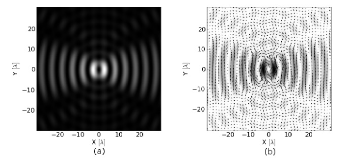
Figure 1: (a) Transverse intensity and (b) electric field of a TE electromagnetic wave with parabolic cylindrical symmetry. The wave parameters are $k_{z}=0.975\omega/c$, $a=0$ and the associated scalar field has even parity. Length is measured in units of the light wavelength $\lambda$.

III Semiclassical force on thermal neutral atoms

Under standard conditions, the interaction between a two level atom and an EM wave with a frequency close to resonance has an electric dipole nature with a coupling factor

$$g^{\pm}=\mu_{12}^{\pm}({\bf e}_{x}\pm i{\bf e}_{y})\cdot{\bf E}.$$

In a semiclassical treatment, the gradient of $g$,

$${\bm{\nabla}}g=({\bm{\alpha}}+i{\bm{\beta}})g,$$

defines the force experienced by the atom. The expression for the average velocity dependent force, valid for both propagating and standing beams, is ashkin :

$$\langle{\bf f}\rangle=\hbar\tilde{\Gamma}p^{\prime}\Big{[}[({\bf v}\cdot{\bm{\alpha}})\frac{1-p}{1+p}+\Gamma/2]{\bm{\beta}}+[({\bf v}\cdot{\bm{\beta}})-\delta\omega]{\bm{\alpha}}\Big{]}.$$ (5)

In this expression

$$\tilde{\Gamma}=\Gamma/[\Gamma(1+p^{\prime})+2{\bf v}\cdot{\bm{\alpha}}[1-p/p^{\prime}-p][p^{\prime}/(1+p)]],$$ (6)

$\Gamma=4k^{3}|{\bm{\mu}}_{12}|^{2}/3\hbar$ is the Einstein coefficient, $\delta\omega=\omega-\omega_{0}$ denotes the detuning between the wave frequency $\omega$ and the transition frequency $\omega_{0}$, $p=2|g|^{2}((\Gamma/2)^{2}+\delta\omega^{2})$ is known as the saturation parameter, linked to the difference $D$ between the populations of the two levels of the atom, $D=1/(1+p)$, and finally $p^{\prime}=2|g|^{2}/|\gamma^{\prime}|^{2}$, with $\gamma^{\prime}=({\bf v}\cdot{\bm{\alpha}})(1-p)(1+p)^{-1}+\Gamma/2+i[({\bf v}\cdot{\bm{\beta}})-\delta\omega]$.

The dissipative term $({\bf v}\cdot{\bm{\beta}})$, associated with a Doppler shift, as well as other velocity dependent terms in Eq. (5) are expected to be small for slow atoms, particularly within the red detuned far-off-resonance regime Miller . In such a case Eq.(5) takes the simpler expression

$$\langle{\bf f}\rangle=\hbar\frac{p}{1+p}\Big{[}\frac{\Gamma}{2}{\bm{\beta}}-\delta\omega{\bm{\alpha}}\Big{]}.$$ (7)

However, we keep the velocity dependent terms in our numerical calculations in order to prevent disregarding potentially relevant effects.

We consider that the cylindrical symmetry axis $z$ of the light field configuration is oriented along the vertical direction and gravity force is included.

IV Atom semiclassical trajectories

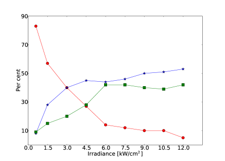
Figure 2: Percentage of non trapping (circles), quasiperiodic (stars) and chaotic trapping (squares) trajectories as a function of the light beam irradiance. The initial conditions for the atomic cloud correspond to random initial positions within a circle of radii $20\lambda$ centered on the axis of the beam and velocities corresponding to a temperature in the range of 2.9-3.1 $\mu$K for the movement in the plane $XY$, perpendicular to the beam, and about 0.2 $\mu$K along the $z$ axis.

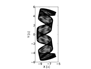
(a)

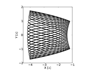
(b)

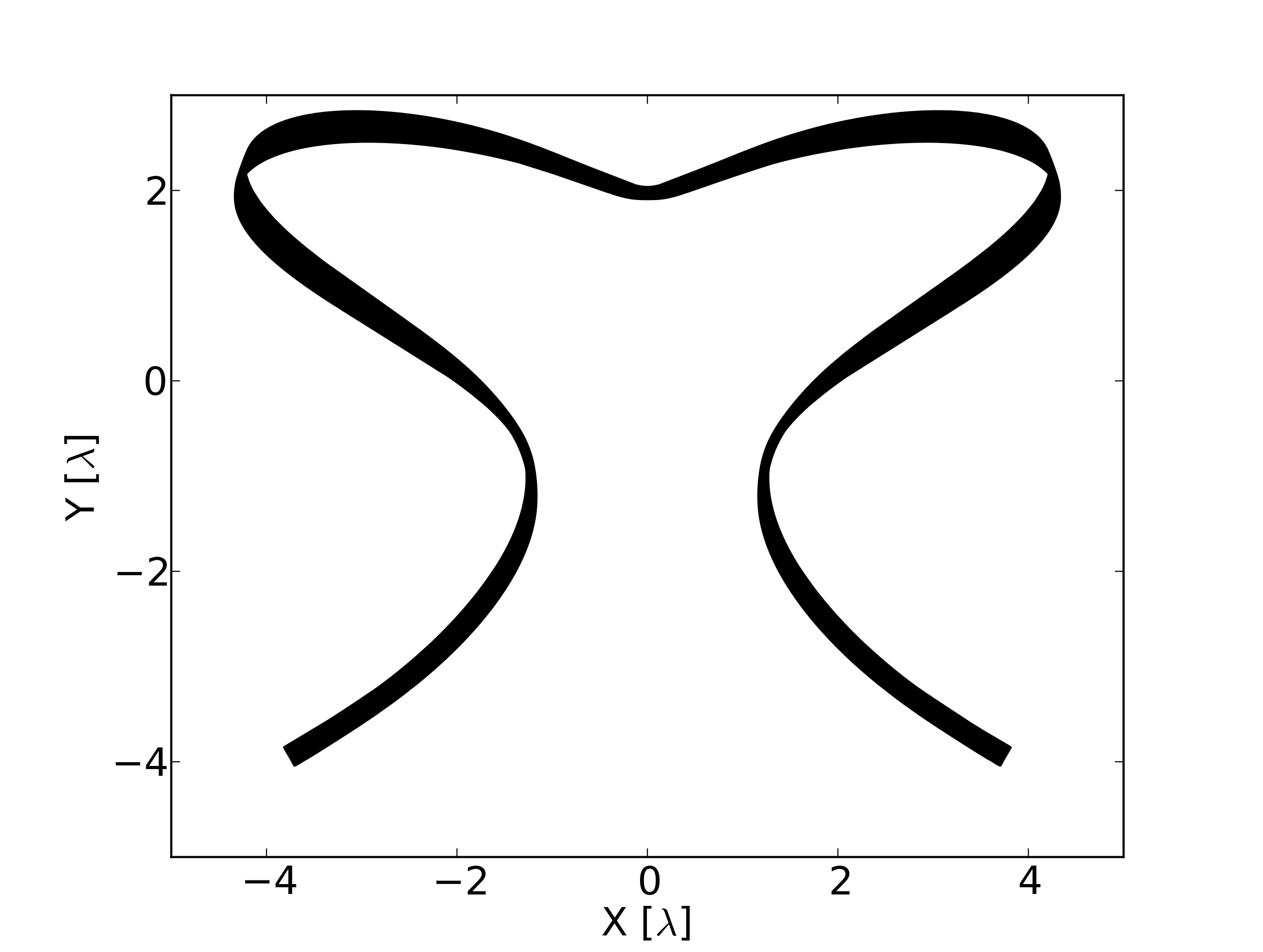
(c)

Figure 3: Three illustrative examples of quasiperiodic trajectories of a cold atom trapped in a parabolic cylinder lattice: (a) the movement takes place within the second lobe to the left of the symmetry axis (see Fig. 1); (b) the movement is confined to a high intensity lobe closest to the symmetry axis; (c) a typical quasiperiodic trajectory that involves more than one optical lobe. For clarity the time interval plotted is a few percentage ($\sim 10\%$) of the 1.25 $\times$ $10^{8}$ $\Gamma^{-1}$ time considered in the numerical calculation. Length is measured in units of the light wavelength $\lambda$.

Figure 4: Power spectra of the coordinate $x(t)$ for the three quasiperiodic trajectories shown in Fig. 3 showing the typical well defined isolated periodicities expected for a regular dynamics. Only the low frequency end of the spectra is shown. The frequency is measured cycles per unit time $\Gamma^{-1}$.

The numerical simulations de consider a TE laser beam detuned 67 nm to the red of the $5\leavevmode\nobreak\ ^{2}S_{1/2}$ - $5\leavevmode\nobreak\ ^{2}P_{1/2}$ transition at $795$ nm of ${}^{85}\text{Rb}$ with irradiance in the range $\sim 0.5-22$ kW/ cm². As natural length and time units, we take the laser wavelength and the inverse of the Einstein coefficient $\Gamma$, which is $3.7\times 10^{7}$s^-1 for the state $5\leavevmode\nobreak\ ^{2}P_{1/2}$ of ${}^{85}\text{Rb}$.

Given an irradiance, initial conditions for a cloud of a hundred non interacting atoms are generated randomly within a circle of radii $20\lambda$ centered on the axis of the beam. The random velocities correspond to a temperature in the range of 2.9-3.1 $\mu$K for the movement in the plane $XY$, perpendicular to the beam, and about 0.2 $\mu$K along the $z$ axis. The anisotropy in the initial velocities enhances the effects of the nontrivial transverse structure since it ”freezes” the z-direction degree of freedom. A mechanism for achieving initial anisotropic velocities at low temperatures could be based in the previous use of a dissipative optical lattice with an anisotropic modulation of the laser-atom interaction parameters sanchez-placencia .

In Figure 2 we illustrate the proportion of non trapped, regular trapped and chaotic trapped trajectories as a function of the irradiance. For instance for an irradiance of $\sim$4.5 kW/cm² about $27\%$ of the atoms are not trapped by the lattice and escape with their route either almost confined in a transverse plane to the beam or with their velocity almost parallel to it. The remaining atoms exhibit a trapped chaotic ($28\%$) or quasi periodic motion ($45\%$). An atom will be considered trapped if for times lower than $1.25\times 10^{8}\Gamma^{-1}$ it remains at a distance to the axis lower than $80\lambda$ while, in the axial direction, it remains within at most $5\lambda$ of its initial $z$ value. An irradiance of $\sim$ 2 kW/cm² is required for trapping $\sim 50\%$ of the atoms. Notice however, that for an irradiance as low as $\sim$0.5 kW/cm² there is a high probability of observing chaotic trajectories within the trapped ones. For an irradiance of $\sim 6$ kW/cm² $\sim 82\%$ of the atoms are trapped by the lattice, about $\sim 35\%$ have a chaotic motion and $\sim 47\%$ a regular one. In the following, the cases that illustrate the atoms dynamics refer to the latter irradiance.

In most of the regular trajectories, the atoms are confined to a single lobe of the lattice (Fig. 3a, 3b) although less than 10$\%$ of the observed regular trajectories can involve two lobes (Fig. 3c) or more than one well along the $z$-direction. We could not find regular trajectories visiting more than two lobes in the XY plane. The quasiperiodic character of the motion can be easily verified by evaluating the power spectra of any of the components of the position or velocity vectors as a function of time as shown in Fig. 4.

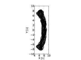
(a)

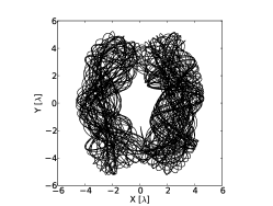
(b)

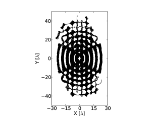
(c)

Figure 5: Three illustrative examples of chaotic trajectories where: (a) the movement takes place within the second lobe to the right of the symmetry axis (see Fig. 1); (b) the movement is confined to the two highest intensity lobes closest to the symmetry axis; (c) the trajectory practically covers the accessible configuration space in the optical lattice. For clarity the time interval plotted is a few percentage ($\sim 10\%$) of the 1.25 $\times$ $10^{8}$ $\Gamma^{-1}$ time considered in the numerical calculation. Length is measured in units of the light wavelength $\lambda$.

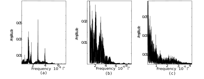
Figure 6: Power spectra of the coordinate $x(t)$ for the three chaotic trajectories shown in Figure 5. The broad band spectra is a signature of chaotic motion. Only the low frequency end of the spectra is shown. The frequency is measured in cycles per unit time $\Gamma^{-1}$.

As for chaotic trajectories, for the initial conditions we considered, they give rise to confined motion within one wavelength in the $z$ direction and transversal motion in either one, two or several lobes in the labyrinths created by the optical lattices in the $XY$ plane, as illustrated in Fig. 5. In the most common chaotic trajectories, the atom remains in a lobe for certain time and then goes to another lobe of the lattice in a very irregular way that practically covers the accessible configuration space in the optical lattice, Fig. 5c.

For atom trajectories involving many lobes, the lobes are visited in an irregular order and an atom can visit the same lobe several times. For Fig. 5c, the atom visits most of the lobes in any interval $(t_{0},t_{0}+\Delta t)$ of duration $\Delta t=1.25\times 10^{7}\Gamma^{-1}$ irrespective of the initial time $t_{0}$.

In Fig. 6 the power spectra of the $x$ coordinate of the trajectories shown in Fig. 5 is presented. The broad band structure of those spectra is a signature of the trajectories chaotic character.

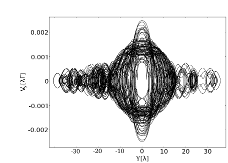
Figure 7: Trajectory in the velocity $V_{y}$ versus position $y$ phase space plane for the path 4c.

Looking for other signatures of chaos, the phase space trajectory can also be also analyzed. In Fig. 7 we illustrate such trajectories in ($y$,$V_{y}$) space. Both Fig. 5c and Fig. 7 point to a dense covering of the accessible phase-space established by the light labyrinth and the atom initial conditions.

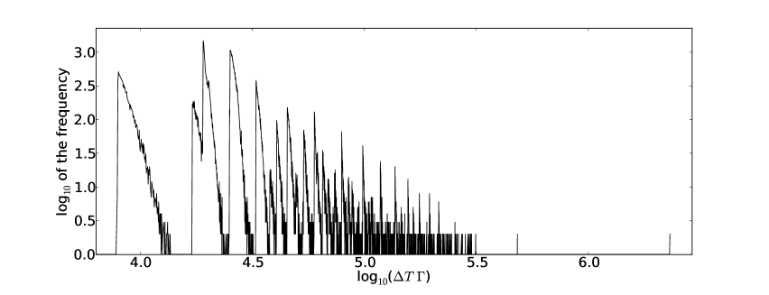
Figure 8: Log–log plot illustrating the statistics of the time an atom expends in an optical lobe before jumping to another optical lobe for a chaotic trajectory. The sampling was taken for the trajectory illustrated in Fig 5b after an analysis that considered a total time $T_{F}=2.5\times 10^{8}\Gamma^{-1}$ in which 82951 transitions took place. The frequency corresponds to the number of events on which the atom expended a time $[T,T+50\Gamma^{-1}]$ within a lobe. The long tail is a signature of a statistics where the momenta is not well defined. In this figure, the logarithm of zero has been mapped to zero.

In Fig. 8, we illustrate the distribution of the permanency time $T_{perm}$ within a lobe in a log-log plot for the trajectory showed in Fig. 5b. The sampling was taken considering a total evolution time $T_{F}=2.5\times 10^{8}\Gamma^{-1}$ in which the atom transits 82951 times from one to the other lobe. Analysis with shorter total evolution time (we studied $T_{F}$ in the interval $[0.5\times 10^{8}\Gamma^{-1},2.5\times 10^{8}\Gamma^{-1}]$) gave frequency distributions of $T_{perm}$ with the same structure; that is (i)the same characteristic minimum time an atom expends within a lobe (a time naturally determined by the initial kinetic energy); (ii) local very stepped maxima followed by strong decays which are then followed by the next maxima; (iii) the longest permanency time $T_{longest}$ has a very small frequency; (iv) if the longest permanency time is not considered the distribution of the local maxima is approximately linear, which would then lead to a power law statistics for that maxima; (v) $T_{longest}$ increases as $T_{F}$ increases. This indicates to us that the momenta of the distribution is not well defined, like in a Levy distribution.

Partial trajectories with nearby values of the permanency time $T_{perm}$ exhibit similarities as illustrated in Figs. 9 and 10. Fig. 9a refers to the trajectories with $T_{perm}$ equal to the minimum time an atom must expend in a lobe. For them, the atom enters through one of the potential maxima and leaves through the other one. In most cases the partial trajectories associated with the local maxima of the distribution, correspond to the ones using the minimum time necessary to transit within a lobe touching a certain number of times the boundary to the other lobe, as illustrated in Fig. 9b. In Fig. 10, we illustrate the type of trajectories with major frequency in the distribution of $T_{perm}$. In this interesting case, we observe the presence of two kind of partial trajectories that go across the lobe entering through one boundary and going out through the same boundary; just one of them almost arrives to the second boundary. The other class of trajectories has a non negligible probability of being followed by an almost identical trajectory under reflection when the atom crosses to the other lobe. This is clearly illustrated in Fig. 10b where consecutive partial trajectories of this kind lead to a partial trajectory very similar to the quasiperiodic case shown in Fig. 3c.

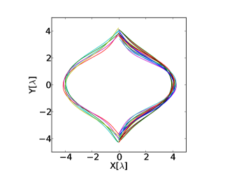
(a)

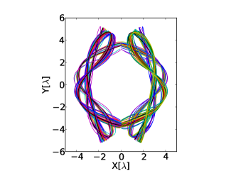
(b)

Figure 9: (Color on line) Illustrative partial trajectories during the time an atom remains within a lobe for the chaotic trajectory shown in Fig. 5b. They were classified according to the time permanency $T_{perm}$ so that in (a) $T_{perm}=8000\pm 1000\Gamma^{-1}$, (b) $T_{perm}=32500\pm 2000\Gamma^{-1}$

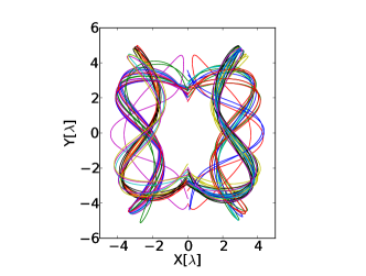
(a)

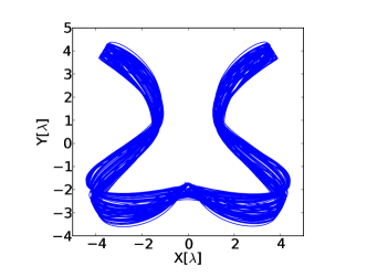
(b)

Figure 10: (Color on line) Illustrative partial trajectories during the time an atom remains within a lobe for the chaotic trajectory shown in Fig. 5b with a permanency time $T_{perm}=19200\pm 1500\Gamma^{-1}$. There is a non negligible probability that the atom passes through this type of partial trajectories in consecutive times as shown in (b).

V Conclusions

We have numerically shown that optical lattices with transverse structure allow the design of potentials yielding non trivial dynamics. For chaotic trajectories, like the one shown in Figure 5c, the atom has a non zero probability to be found at any point within its accessible region of phase space. This behavior is similar to that expected for the quantum description of the atom motion. In this case the atom wave function will necessarily lead to a position probability density that mimics the optical structure, being non zero in any of the lobes. We expect that for ultra cold atoms chaos-assisted bidimensional tunneling will take place.

Under the proposed set-up, one can notice that the fraction of trapped atoms with chaotic trajectories diminishes as the irradiance is lowered, Fig. 2. It is also important to emphasize that, for intermediate values of the irradiance, most of the trapped chaotic trajectories involve more than one lobe and that the distribution of time permanencies within a lobe is highly structured and with a long tail. Finally, for high irradiances, the proportion of chaotic trajectories saturates and there is a high presence of quasiperiodic trajectories. In this last regime, the atom is highly confined in the $z$-direction and tends to move inside a single optical potential lobe. Since the detuning is large, dissipative effects are expected to be small, thus, in the high intensity regime, the system dynamics is very similar to that of two-dimensional billiards with a topology determined by the parabolic symmetry of the light beam. It is knownquasi-bill that this kind of dynamical systems have a large set of quasiperiodic solutions. We consider this the key to understand the saturation effect illustrated in Fig. 2.

Notice that the use of a propagation invariant EM wave is not mandatory for the qualitative results we found. The use of other beams like the Gaussian parabolic are expected to yield similar results for the transverse motion of atoms in the focusing plane.

We also assumed anisotropic initial velocities. If the mean initial z-velocity were comparable with the transverse velocities, one would expect that the atoms motion would take place in multiple quasi bidimensional configuration spaces since the atom would visit several of the sinusoidal potential wells in the z-direction. However, the projection of the trajectories in a given transversal plane would be expected to be qualitatively similar to those described above.

For the geometries we are studying, blue detuned beams, due to the numerous routes of escape provided by the dark light zones, in general do not lead to trapped trajectories. Nevertheless this scattering process deserves a detailed study on its own, both classically and quantum mechanically.

References

- (1) F. Bardou, J. P. Bouchaud, O. Emile, A. Aspect, and C. Cohen-Tannoudji 1994 Phys. Rev. Lett. 72 203; J. C. Robinson, C. Bharucha, F. L. Moore, R. Jahnke, G. A. Georgakis, Q. Niu, M. G. Raizen, and B. Sundaram 1995 Phys. Rev. Lett. 74 3963; C. Jurczak, B. Desruelle, K. Sengstock, J. Y. Courtois, C. I. Westbrook, and A. Aspect 1996 Phys. Rev. Lett. 77 1727; S. Marksteiner, K. Ellinger, P. Zoller 1996 Phys. Rev. A 53 3409; H. Katori, S. Schlipf, and H. Walther 1997 Phys. Rev. Lett. 79 2221; B. G. Klappauf, W. H. Oskay, D. A. Steck, and M. G. Raizen 1998 Phys. Rev. Lett. 81 4044
- (2) F. L Moore, J. C. Robinson, C. Bharucha, P. E. Williams, and M. G. Raizen 1994 Phys. Rev. Lett. 73 2974
- (3) D.A. Steck, W.H. Oskay, and M.G. Raizen 2001 Science 293 274; D. A. Steck, W. H. Oskay, and M. G. Raizen 2002 Phys. Rev. Lett. 88 120406
- (4) V. Yu. Argonov and S. V. Prants 2008 Phys. Rev. A 78 043413
- (5) J. P. Bouchaud and A. Georges 1990 Phys. Rep. 195, 127; M. F. Shlesinger, G. M. Zaslavsky, and J. Klafter 1993 Nature (London) 363 31
- (6) S. Tomsovic and D. Ullmo 1994 Phys. Rev. E 50 145; W. A. Lin and L. E. Ballentine 1990 Phys. Rev. Lett. 65 2927; R. Utermann, T. Dittrich, and P. Hänggi 1994 Phys. Rev. E 49 273
- (7) V. Milner, J. L. Hanssen, W. C. Campbell, and M. G. Raizen 2001 Phys. Rev. Lett. 86 1514
- (8) N. Friedman, A. Kaplan, D. Carasso, and N. Davidson 2001 Phys. Rev. Lett. 86 1518
- (9) M. F. Andersen, A. Kaplan, N. Friedman, and N. Davidson 2002 J. Phys. B: At. Mol. Opt. Phys. 35 2183
- (10) M. F. Andersen, A. Kaplan, and N. Davidson 2003 Phys. Rev. Lett. 90 023001; M. F. Andersen, A. Kaplan, T. Grünzweig, and N. Davidson 2006 Phys. Rev. Lett. 97 104102
- (11) A. Kaplan, N. Friedman, M. Andersen, and N. Davidson 2001 Phys. Rev. Lett. 87 274101
- (12) J. C. Gutiérrez-Vega, M. D. Iturbe-Castillo, and S. Chávez-Cerda 2000 Opt. Lett. 25 1493; M. B. Alvarez-Elizondo, R. Rodríguez-Masegosa, and J. C. Gutiérrez-Vega 2008 Opt. Express 16 18770
- (13) L. Allen, M. W. Beijersbergen, R. J. C. Spreeuw, and J. P. Woerdman 1992 Phys. Rev. A 45 8185; M. Babiker, C. R. Bennett, D. L. Andrews, and L. C. Davila-Romero 2002 Phys. Rev. Lett. 89 143601; L. Amico, A. Osterloh, and F. Cataliotti 2005 Phys. Rev. Lett. 95 063201; A. Alexandrescu, D. Cojoc, E. Di Fabrizio 2006 Phys. Rev. Lett. 96 243001; M. Bhattacharya 2007 Opt. Commun. 279 219; S. E. Olson, M. L. Terraciano, M. Bashkansky, and F. K. Fatemi 2007 Phys. Rev. A 76 061404R
- (14) J. W. R. Tabosa and D. V. Petrov 1999 Phys. Rev. Lett. 83 4967
- (15) G. S. Paraoanu 2003 Phys. Rev. A 67 023607 ; M. F. Andersen, C. Ryu, P. Clade, V. Natarajan, A. Vaziri, K. Helmerson, W. D. Phillips 2006 Phys. Rev. Lett. 97 170406
- (16) J. Durnin, J. J. Miceli, and J. H. Eberly 1987 Phys. Rev. Lett. 58 1499; J. Arlt and K. Dholakia, Opt. Commun. 177, 297 (2000); K. Volke-Sepúlveda, R. Jáuregui 2009 J. Phys. B: At. Mol. Opt. Phys. 42 085303
- (17) J. C. Gutiérrez-Vega, M. D. Iturbe-Castillo, G. A. Ramírez, E. Tepichín, R. M. Rodríguez-Dagnino, S. Chávez-Cerda and G. H. C. New 2001 Opt. Commun. 195 35; S. Chávez-Cerda, M. J. Padgett, I. Allison, G. H. C. New, J. C. Gutiérrez-Vega, A. T. O’Neil, I. MacVicar, and J. Courtial 2002 J. Opt. B: Quantum Semiclassical Opt. 4 S52S57; B. M. Rodríguez-Lara and R. Jáuregui 2008 Phys. Rev. A 78 033813
- (18) N. N. Lebedev 1972 Special Functions and their Applications (Dover Publications: U. S. A.)
- (19) B. M. Rodríguez-Lara and R. Jáuregui 2009 Phys. Rev. A 79 055806
- (20) C. López-Mariscal, M. A. Bandres, and J. C. Gutiérrez-Vega 2005 Opt. Exp. 13 2364
- (21) J. A. Davis, M. J. Mintry, M. A. Bandres, and D. M. Cottrell 2008 Opt. Exp. 16 12866
- (22) V. S. Letokhov and V. G. Minogin 1978 Appl. Phys. 17 99; J. P. Gordon and A. Ashkin 1980 Phys. Rev. A 21 1606
- (23) J. D. Miller, R. A. Cline, and D. J. Heinzen 1993 Phys. Rev. A 47 R4567
- (24) The differential equations solver corresponds to the double precision LSODE subroutine by A. Hindmarsh and L. Petzhold in the public library ODEPACK.
- (25) J. Jersbland, H. Ellmann, L. Sanchez-Placencia, and A. Kastberg 2003 Eur. Phys. J. D 22 333
- (26) V. Zharnitsky 1998 Phys. Rev. Lett. 81 4839