kcl-mth-10-22, arxiv:1012.3996
overview article: arxiv:1012.3982

Review of AdS/CFT Integrability, Chapter III.7:
Hirota Dynamics for Quantum Integrability

Nikolay Gromov^a, Vladimir Kazakov^b

^a King’s College, London Department of Mathematics WC2R 2LS, UK
St.Petersburg INP, St.Petersburg, Russia
^b Ecole Normale Superieure, LPT, 75231 Paris CEDEX-5, France
l’Université Paris-VI, Paris, France

^anikolay.gromov@kcl.ac.uk

Abstract:

We review recent applications of the integrable discrete Hirota dynamics (Y-system) in the context of calculation of the planar AdS/CFT spectrum. We start from the description of solution of Hirota equations by the Bäcklund method where the requirement of analyticity results in the nested Bethe ansatz equations. Then we discuss applications of the Hirota dynamics for the analysis of the asymptotic limit of long operators in the AdS/CFT Y-system.

1 Introduction

The Hirota integrable hierarchy [1] enables us to take a very general point of view on integrability, in classical systems [2] as well as in 2D statistical mechanical [3] and quantum systems [4, 5, 6]. The analytic Bethe ansatz approach based on the Y- and T-systems for the fusion of transfer-matrices in various representations was successfully applied to various spin chains and 2D QFT’s [6, 7] and is especially efficient for the supersymmetric systems [8, 9, 10]. Being integrable, Hirota equation with specific boundary conditions stemming from the symmetry of the problem, can be often solved explicitly, either by the Bäcklund method [6, 9] or in the determinant (Wronskian) form [6, 11]. Of course to specify completely the physical solutions we have to precise the functional space for the functions of spectral parameter entering Hirota equation, or in other words, we also need to impose certain analyticity conditions on these solutions which is usually the hardest part of the problem. In the spin chains the role of analyticity conditions is usually played by the polynomiality of the transfer-matrices, resulting in supplementary conditions - the Bethe ansatz equations. For the Y-systems of integrable 2D QFT’s (sigma models) at a finite volume, the analyticity imposes the absence of singularities on a physical domain of the complex plane of a spectral parameter, except those related to various physical excitations (see [12] for the example of $O(4)$ sigma model).

These methods, based on the Hirota integrable dynamics, recently have shown again their power in the problem of calculation of the exact conformal dimensions in the planar N=4 SYM theory. The program of integrability for the spectrum in planar AdS/CFT correspondence has lead to the discovery of a system of exact spectral equations — the Y-system — containing an important information about the anomalous dimensions of all local operators at arbitrary ’t Hooft coupling. The AdS/CFT Y-system and the underlying integrable Hirota equation were first conjectured in a functional form [13] and later reproduced in the form of an infinite system of non-linear integral equations [14, 15, 16] from the TBA approach [4]. It was successfully tested analytically in the weak coupling regime, in particular for Konishi operator and twist-2 operators by the direct 4-loop perturbation theory, and even up to 5 loops, comparing with the BFKL approximation [17], and in the strong coupling for long operators, by comparison with quasi-classical string theory results [18, 19]. The first numerical study of Konishi dimension [20] in a wide range of couplings (see Fig.2 of [21]), showed a perfect interpolation between the $N=4$ SYM perturbation theory and the SYM strong coupling asymptotics described by the large radius of the superstring $AdS_{5}\times S^{5}$ background [22].

In this paper, we will introduce the reader into the basics of Hirota approach to the quantum integrability on the example of AdS₅/CFT₄ duality. But first we will show how to solve, following the methods of [9, 23, 6, 8], Hirota equation for the fusion in the rational supersymmetric spin chains with $gl(N|M)$ symmetry, in terms of a generating functional (generalized Baxter equations) by means of the Bäcklund method, and to derive the nested Bethe ansatz equations. Then we will follow this logic in the AdS/CFT system and try to show that the worldsheet scattering theory and asymptotic Bethe ansatz ABA for the superstring on AdS₅/CFT₄ background are also tightly related to the analyticity of the Y-system whose form, in its turn, is greatly constrained by the superconformal $psu(2,2|4)$ symmetry of the theory.

2 Hirota Equations in the $gl(N)$ spin chain

The simplest example where the Hirota equation appears naturally is the generalized Heisenberg $gl(N)$ spin chain for compact representations. The spin chain Hamiltonian and all other conserved charges can be constructed from the R-matrix [24]. We give in this section the basics of the analytic Bethe ansatz approach to this system following [9, 10, 23].

Our the explanations (though not the proofs) will be self-contained, all the way from the R-matrix to the Hirota equation. The R-matrix of $gl(N)$ super-spin chain is

$$R_{\lambda}(u)=u\,\,\mathbb{I}\ \otimes\mathbb{I}_{\lambda}+i\sum_{\alpha,\beta=1}^{N}e_{\beta\alpha}\otimes\pi_{\lambda}(e_{\alpha\beta})\,,$$ (2.1)

Figure 1: A: $R$-matrix in pictures; B: Yang-Baxter relation; C: Transfer matrix

where the generators in the l.h.s.(r.h.s.) of the tensor product in each term correspond to the “physical” (“auxiliary”) space and $\lambda$ refers to an arbitrary representation in the “auxiliary” space. $\mathbb{I}$ and $\mathbb{I}_{\lambda}$ are the identity elements in fundamental representation and in representation $\lambda$, respectively; $e_{\alpha\beta}$ are the generators of $u(N)$ algebra acting in the fundamental representation on the basis $e_{\gamma}$ as $e_{\alpha\beta}e_{\gamma}=e_{\alpha}\delta_{\beta\gamma}\;,$ and $\pi_{\lambda}(e_{\alpha\beta})$ are the same generators in any irrep $\lambda$. In $\lambda$ fundamental, the second term $\mathcal{P}\equiv\sum_{\alpha\beta}e_{\beta\alpha}\otimes e_{\alpha\beta}\,,$ becomes simply the permutation operator and it is easy to check that the R-matrix satisfies the Yang-Baxter equation

$$R_{12}(u)R_{13}(u+v)R_{23}(v)=R_{23}(v)R_{13}(u+v)R_{12}(u)$$ (2.2)

where the operators act on the tensor product of $3$ fundamental physical states and the lower indexes show on which of the states the action of $R$ is nontrivial (see Fig.1B).

Next, we introduce the transfer matrix as a trace in the auxiliary space of irrep $\l$ of the monodromy matrix (see the Fig.1C):

$$\hat{T}_{\lambda}(u,g)\equiv{\rm tr_{aux}}\,\left(R_{\lambda}(u)^{\otimes L}\pi_{\lambda}(g)\right)\,,$$

where the tensor products are taken for the physical spaces and the usual matrix product and the trace refers to the the auxiliary space, $\pi_{\lambda}(g)$ being a group element $g$ in the irrep $\l$. The transfer matrix $\hat{T}_{\lambda}(u,g)$ is thus an operator acting on $L$ copies of the physical space, i.e. on the Hilbert space of the spin chain with $L$ cites. Notice that for $L=0$ the transfer matrix is simply a character $\chi_{{}_{\lambda}}(g)$.

To relate the transfer matrices to the group characters, we introduce a useful operator called the co-derivative ${\cal D}$ [10] defined by the action on a function of $g$:

$${\cal D}f(g)=e_{\beta\alpha}\left.\frac{\partial}{\partial\phi_{\alpha\beta}}f\left(e^{\phi_{\delta\gamma}e_{\delta\gamma}}g\right)\right|_{\phi=0}\,,\quad{\rm where}\qquad\frac{\partial}{\partial\phi_{\alpha_{1}\beta_{1}}}\phi_{\alpha_{2}\beta_{2}}\equiv\delta_{\alpha_{1}\alpha_{2}}\delta_{\beta_{1}\beta_{2}}\,.$$ (2.3)

In particular, applying it to (2.1), we rewrite the transfer matrix in an instructive way

$$\hat{T}_{\lambda}(u)=(u+i{\cal D})^{\otimes L}\chi_{{}_{\lambda}}(g)\;.$$ (2.4)

In what follows we consider only the representations $\l=s^{a}$ with rectangular Young diagrams $\lambda_{i}=s,\;i=1,\dots,a$. Below we demonstrate that the transfer matrices with different spectral parameters $u$ and irreps $\lambda$ commute with each other and thus we can work with their eigenvalues denoted below as $T_{\lambda}(u)$. We denote $\chi_{{}_{a,s}}\equiv\chi_{s^{a}}$ and

$$\hat{T}_{a,s}(u)\equiv\frac{\hat{T}_{{}_{s^{a}}}(u+\tfrac{s-a}{2i})}{(u+\tfrac{s-a}{2i})^{L}}$$ (2.5)

where we chose the normalization of the eigenvalues

$$T_{a,0}=T_{0,s}=1\;.$$ (2.6)

The goal of this section is to demonstrate the following Hirota equation [3, 6]:

$$T_{a,s}(u+\tfrac{i}{2})T_{a,s}(u-\tfrac{i}{2})=T_{a+1,s}(u)T_{a-1,s}(u)+T_{a,s+1}(u)T_{a,s-1}(u)$$ (2.7)

Let us demonstrate the validity of (2.7) on the case $a=1$. The symmetric characters $\chi_{{}_{1,s}}(g)$ are generated as the Schur polynomials from the generating function

$$\\ w(z)=\det(1-zg)^{-1}=\sum_{s=0}^{\infty}z^{s}\chi_{{}_{1,s}}.$$ (2.8)

Acting on $w(z)$ by the left co-derivative we easily find that

$${\cal D}\log w(z)=\frac{zg}{1-zg}$$ (2.9)

$$(1+{\cal D})w(z_{1}){\cal D}w(z_{2})=\frac{1}{1-z_{1}g}\frac{z_{2}g}{1-z_{2}g}=\frac{z_{2}}{z_{1}}\frac{z_{1}g}{1-z_{1}g}\frac{1}{1-z_{2}g}=\frac{z_{2}}{z_{1}}\,{\cal D}w(z_{1})(1+{\cal D})w(z_{2})\;.$$ (2.10)

The last equation in particular implies the following relation among the characters

$${\cal D}\chi_{1,s}(\chi_{s}+{\cal D}\chi_{s})={\cal D}\chi_{1,s+1}(\chi_{s-1}+{\cal D}\chi_{s-1})$$ (2.11)

which, for the simple one spin chain $L=1$, is equivalent to a particular case of (2.7)

$$\hat{T}_{1,s}(u+\tfrac{i}{2})\hat{T}_{1,s}(u-\tfrac{i}{2})=\hat{T}_{0,s}(u)\hat{T}_{2,s}(u)+\hat{T}_{1,s-1}(u)\hat{T}_{1,s+1}(u)$$ (2.12)

where we had to use that $\chi_{2,s}=\chi_{1,s}^{2}-\chi_{1,s+1}\chi_{1,s-1}$ and $\chi_{0,s}=1$. Moreover, one can see that the one spin transfer matrices are a combinations of only $g$ and the unit matrix and thus commute with each other. We send the interested reader to [10] for the general proof of the Hirota relation (2.7) for any irrep and any number of spins. Eq.(2.7) is a generalization of a similar, but simplified, Hirota relation among the characters: $\chi_{{}_{a,s}}^{2}=\chi_{{}_{a+1,s}}\chi_{{}_{a-1,s}}+\chi_{{}_{a,s+1}}\chi_{{}_{a,s-1}}$ - following from the multiplication of rectangular irreps.

It is remarkable that the fusion equation (2.7) is the same for all $gl(N)$ groups. Different $N$ will correspond however to different boundary conditions. In particular, one has $T_{N+1,s}=0$ (as well as $T_{a<0,s}=T_{a\neq 0,s<0}=0$), $T_{a<0,s}=T_{a\neq 0,s<0}=0$ which is clear from the same conditions for the characters: $\chi_{N+1,s}=0$. It turns out that for the super groups $gl(N|M)$ the Hirota equation is again the same whereas the nonzero $T_{a,s}$ belong to so called fat-hook [8] (see Fig.2a).

It is easy to check that the “gauge” transformation

$$T_{a,s}\to g_{1}^{[a+s]}g_{2}^{[a-s]}g_{3}^{[s-a]}g_{4}^{[-a-s]}T_{a,s}$$ (2.13)

where $g_{i}$ are arbitrary functions, leaves the form of the Hirota equation unchanged. One may choose certain normalization of the solutions by fixing these functions in one or another way, as we do in (2.6). Notice that (2.6) still leaves one gauge degree of freedom unfixed. We can also introduce the quantities gauge invariant w.r.t. (2.13)

$$Y_{a,s}=\frac{T_{a,s+1}T_{a,s-1}}{T_{a+1,s}T_{a-1,s}}\;$$ (2.14)

As a consequence of Hirota equations (2.7) they satisfy the discrete Y-system equations

$$Y_{a,s}^{+}Y_{a,s}^{-}=\frac{(1+Y_{a,s+1})(1+Y_{a,s-1})}{(1+1/Y_{a+1,s})(1+1/Y_{a-1,s})}\;.$$ (2.15)

There exists a concise solution of Cauchy problem for Hirota equation in the semi-$(a,s)$-plane , in terms of $T_{1,s}(u)$ fixed along the boundary (recall that $T_{0,s}(u)=1$ in our gauge), the so called Bazhanov-Reshetikhin determinant formula [25, 10] for the fusion in spin chains (valid here in a more general context)

$$T_{a,s}=\det_{1\leq j,k\leq a}T_{1,s+k-j}\left(u+\tfrac{k+j-a-1}{2i}\right)\;.$$ (2.16)

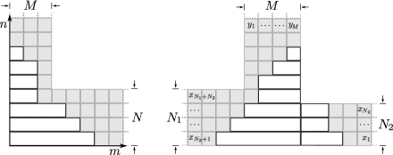
Figure 2: The fat-hook for the representations of $SU(N|M)$ (left) and $\mathbb{T}$-hook for the representations of $SU(N_{1},N_{2}|M)$ (right). The lengths of horizontal (white) strips forming the Young tableau of an irrep are equal to its highest weight components.

Our strategy will be to get as much information as possible about the system by solving the Hirota equations. The Bethe ansatz equations naturally appear in this approach as a requirement of analyticity, or, in the case of spin chains, of polynomiality of all transfer-matrices. In the next section we show how the Hirota classical integrable discrete dynamics helps to solve, by means of the Bäcklund transform, the fusion relations (2.7) in terms of a generating functional.

3 Integrability of Hirota Equations

In this section we describe the general solution of Hirota equations in the $(N|M)$ fat hook shown on the Fig.2. We apply for that the Bäcklund transformation technique based on the classical integrability of discrete Hirota dynamics, and show how it helps to solve the problem by gradually reducing the $(N|M)$ fat hook to a trivial one $(0|0)$. As a result we derive the generating functional for the general solution of Hirota equations. In particular, the polynomial solution corresponds to the transfer matrices of the $SL(N|M)$ rational Heisenberg super-spin chain described above.

3.1 Linear system for Hirota equation

The classical integrability for the Hirota dynamics manifests itself in the existence of an axillary linear problem - a pair of Lax equations

$${\rm eq}^{I}_{a,s}(u)\;\;:\;\;T_{a+1,s}F^{+}_{a,s} = +x\;T_{a+1,s-1}^{+}F_{a,s+1}+T_{a,s}^{+}F_{a+1,s}\;\;,$$

$${\rm eq}^{II}_{a,s}(u)\;\;:\;\;T_{a,s-1}F^{+}_{a,s} = -x\;T_{a+1,s-1}^{+}F_{a-1,s}+T_{a,s}^{+}F_{a,s-1}\;\;.$$ (3.1)

Their compatibility condition gives the Hirota equation (2.7). Indeed, we notice that $F_{a,s}^{++}$ can be expressed through $F_{a+1,s-1},\;F_{a,s},\;F_{a-1,s+1}$ in two different ways: 1) use ${\rm eq}^{I}_{a,s}(u+\tfrac{i}{2})$ and then ${\rm eq}^{II}_{a,s+1}(u)$ with ${\rm eq}^{II}_{a+1,s}(u)$ 2) use ${\rm eq}^{II}_{a,s}(u+\tfrac{i}{2})$ and then ${\rm eq}^{I}_{a-1,s}(u)$ with ${\rm eq}^{I}_{a,s-1}(u)$. If we subtract the two results only the term linear in $x$ survives which implies:

$$\frac{T_{a,s}^{+}T_{a+1,s-2}}{T_{a,s-1}T_{a+1,s-1}^{-}}+\frac{T_{a,s}^{+}T_{a+2,s-1}}{T_{a+1,s}T_{a+1,s-1}^{-}}-\frac{T_{a+1,s-1}^{+}T_{a-1,s}}{T_{a,s-1}T^{-}_{a,s}}-\frac{T_{a+1,s-1}^{+}T_{a,s+1}}{T_{a+1,s}T_{a,s}^{-}}=0$$ (3.2)

or, to put it differently, the function defined by $f_{a,s}=\frac{T_{a-1,s}T_{a+1,s}+T_{a,s-1}T_{a,s+1}}{T_{a,s}^{+}T_{a,s}^{-}}$ should be periodic under the shift $f_{a,s}(u)=f_{a+1,s-1}(u)$. Since for the transfer matrices $T_{0,s}=1$ this implies that $f_{0,s}=1$ and thus $f_{a,s}\equiv 1$, leading to Hirota eq. (2.7).

Next, noticing that the Hirota equation is invariant under $(a,s,u)\to(-a,-s,-u)$ we can easily find another linear system (useful for the next section)

$$T_{a-1,s}\tilde{F}^{-}_{a,s} = +y\;T_{a-1,s+1}^{-}\tilde{F}_{a,s-1}+T_{a,s}^{-}\tilde{F}_{a-1,s}\;\;,$$

$$T_{a,s+1}\tilde{F}^{-}_{a,s} = -y\;T_{a-1,s+1}^{-}\tilde{F}_{a+1,s}+T_{a,s}^{-}\tilde{F}_{a,s+1}\;.$$ (3.3)

3.2 Solution of Hirota fusion equation by the Bäcklund method

As it was announced above the Bäcklund method allows to reduce the Hirota equation in a fat-hook $(N|M)$ to the same equation in a smaller fat hook $(n|m)$ with $n\leq N,\;m\leq M$. For that we notice that (3.1), after the appropriate shifts in the spectral parameter and in $a$ and $s$, can be written in the form

$$F_{a-1,s}T^{-}_{a,s} = +x\;F^{-}_{a-1,s+1}T_{a,s-1}+F^{-}_{a,s}T_{a-1,s}\;\;,$$

$$F_{a,s+1}T^{-}_{a,s} = -x\;F^{-}_{a-1,s+1}T_{a+1,s}+F^{-}_{a,s}T_{a,s+1}$$ (3.4)

which is precisely the second linear system (3.1) with $F_{a,s}$ and $T_{a,s}$ interchanged. In particular, this implies that $F_{a,s}$ should also satisfy the same Hirota equation. It is always possible to choose $F_{a,s}$ so that it satisfies Hirota equation in a smaller fat-hook $(N-1|M)$ i.e. to have $F_{N,s}=0\;\;,\;\;s>M.$ One can immediately see from (3.2) that this condition is compatible with the fat hook boundary condition for T-functions $T_{N+1,s>M}=0$. Below we will construct this solution explicitly.

In view of this symmetry between $F$ and $T$ we can denote $T^{N|M}_{a,s}=T_{a,s}$ and $T^{N-1|M}_{a,s}\propto F_{a,s}$ with a particular normalization (2.13): we normalize them so that $T_{0,s}=1$ and $T_{a,0}=1$. From (3.1), this normalization implies for $F$ the following relations $F_{0,s+1}=F^{-}_{0,s}\;\;,\;\;F_{a-1,0}=F^{-}_{a,0}$ which means that we can express $F_{0,s}$ or $F_{a,0}$ in terms of $F_{0,0}$ with a shifted argument $F_{0,s}=F_{0,0}(u-i\tfrac{s}{2}),\;\;F_{a,0}=F_{0,0}(u+i\tfrac{a}{2})\;.$ Thus in our normalization we get $T_{a,s}^{N-1|M}\equiv\frac{F_{a,s}(u)}{F_{0,0}(u+\tfrac{s-a}{2i})}\;$. It should be also clear that due to the symmetry between $F$ and $T$ we can change the logic and tell that (3.1) allows to increase $M$. Similarly, the second linear system (3.1) allows to decrease $M$ (or increase $N$) and we denote $T_{a,s}^{N|M-1}\equiv\frac{\tilde{F}_{a,s}(u)}{\tilde{F}_{0,0}(u+\tfrac{s-a}{2i})}\,$.

By making an appropriate chain of these two transformations we can always reduce a fat hook ($N|M)$ to the trivial one $(0|0)$, through a set of the intermediate fat hooks $(n|m),\quad 0<n<N;0<m<M$ (see fig.3). This procedure allows to write the solution quite explicitly. For the next section we introduce the parameterization

$$\frac{F_{0,0}^{--}}{F_{0,0}}\,=\frac{{\cal Q}_{N|M}^{++}{\cal Q}_{N-1|M}^{--}}{{\cal Q}_{N|M}{\cal Q}_{N-1|M}}\;\;,\;\;\frac{\tilde{F}_{0,0}^{++}}{\tilde{F}_{0,0}}\,=\frac{{\cal Q}_{N|M}^{--}{\cal Q}_{N|M-1}^{++}}{{\cal Q}_{N|M}{\cal Q}_{N|M-1}}$$ (3.5)

The above equations define ${\cal Q}_{N|M-1}$ and ${\cal Q}_{N-1|M}$ in terms of ${\cal Q}_{N|M}$, for given functions $F_{0,0},\tilde{F}_{0,0}$. Since our normalization (2.6) allows for one more gauge one can set ${\cal Q}_{N|M}$ to $1$. This, however, is not the most convenient choice. In the case of spin chains (as in section 2) a natural chose is ${\cal Q}_{N|M}=\prod_{j=1}^{L}(u-\theta_{j})$. In this normalization, at an arbitrary step, or nesting level $(n|m)$ of our Bäcklund procedure, ${\cal Q}_{n|m}$ will be a polynomial, the denominator of the rational functions $T_{a,s}^{n|m}(u-\tfrac{s-a}{2i})$ (like in (2.5)).

Furthermore we denote

$${\cal X}_{n|m}=x_{n}\frac{{\cal Q}_{n|m}^{++}{\cal Q}_{n-1|m}^{--}}{{\cal Q}_{n|m}{\cal Q}_{n-1|m}}\;\;,\;\;{\cal Y}_{n|m}=y_{m}\frac{{\cal Q}_{n|m}^{--}{\cal Q}_{n|m-1}^{++}}{{\cal Q}_{n|m}{\cal Q}_{n|m-1}}\;.$$ (3.6)

3.3 A recurrent equation for the generating functional

For the quantum generalization of the generating function for the characters (2.8) we introduce an operator valued functional

$${\cal W}^{n|m}=\sum_{s=-\infty}^{\infty}D^{s}T^{n|m}_{1,s}(u)D^{s}$$ (3.7)

where $D$ is a shift operator defined by $Df(u)=f(u-\tfrac{i}{2})D$. From (3.1) at $a=0$ we get in notations (3.6)

$$T^{n-1|m}_{1,s}(u) = T^{n|m}_{1,s}(u)-{\cal X}_{n|m}(u+\tfrac{s-1}{2i})\;T_{1,s-1}^{n|m}(u+\tfrac{i}{2})$$ (3.8)

where we introduced new $n|m$ indices for $F$ characterizing the “level” on which we make this Bäcklund transformation. This implies

$${\cal W}^{n-1|m}={\cal W}^{n|m}\left(1-D{\cal X}_{n|m}D\right)$$ (3.9)

and similarly

$${\cal W}^{n|m}={\cal W}^{n|m-1}\left(1-D{\cal Y}_{n|m}D\right)\;.$$ (3.10)

Using the relations (3.9) and (3.10) we can show that any solution of Hirota equation in the $(N|M)$ fat hook can be explicitly and concisely written in the form of a simple generating functional. For that we have to apply the recursions (3.9) and (3.10) along a path of the length $N+M$ on the $(n|m)$ lattice, connecting the upper right and the lower left corners of the $N\times M$ rectangle on Fig.3. This gives the following formula for the generating functional (3.7) [6, 8, 9]

$${\cal W}^{N|M}=\overleftarrow{\prod_{{\rm path}}}\left\{\begin{array}[]{ll}(1-D{\cal X}_{n|m}D)^{-1}&,\;\;{\rm vertical}\\ (1-D{\cal Y}_{n|m}D)&,\;\;{\rm horizontal}\\ \end{array}\right.$$ (3.11)

where the subset of $N+M$ functions ${\cal X}_{n|m},\;{\cal Y}_{n|m}$, chosen out of the whole set of $N\times M$ such functions, depends on the path (see Fig.3).

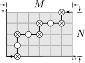
Figure 3: Bäcklund procedure: a possible reduction path on the $(n|m)$-lattice.

$${\cal X}_{n|m}\;\;,\;\;\text{line from}\;(n,m)\;\text{to}\;(n-1,m)$$ (3.12)

$${\cal Y}_{n|m}\;\;,\;\;\text{line from}\;(n,m)\;\text{to}\;(n,m-1)$$ (3.13)

In the case when ${\cal Q}_{n|m}$ are polynomials the solution of Hirota equation constructed in this way corresponds to the transfer matrices with a twist given by a supergroup element $g={\rm diag}\{x_{1},\dots,x_{N}|y_{1},\dots,y_{M}\}$.

3.4 Analyticity and Bethe ansatz equations

The parameterization of a solution of Hirota equation in terms of ${\cal Q}$-functions described above is very convenient for constructing solutions with particular analytic properties. In this section we assume that ${\cal Q}_{n|m}$ are some functions without poles, more general than polynomials, which could have some zeros. Generically, in the process of the Bäcklund construction of a solution these zeros will create poles in the T-functions. However it is possible to cancel all the poles in all $T$-functions by adjusting accordingly the zeros of the ${\cal Q}_{n|m}$ functions. This will lead to a set of nested Bethe ansatz equations.

To get it we notice that if ${\cal Q}_{n|m}$ has a zero $u^{(n|m)}_{j}$ then two vertical links in the path in fig.3 meeting at the point $(n|m)$ give the following (explicitly written) factor in the generating functional

$${\cal W}\simeq\dots\times(1-D{\cal X}_{n|m}D)^{-1}(1-D{\cal X}_{n+1|m}D)^{-1}\times\dots=$$ (3.14)

$$\dots\times\left[1-D\left(x_{n}\frac{{\cal Q}_{n|m}^{++}{\cal Q}_{n-1|m}^{--}}{{\cal Q}_{n|m}{\cal Q}_{n-1|m}}+x_{n+1}\frac{{\cal Q}_{n+1|m}^{++}{\cal Q}_{n|m}^{--}}{{\cal Q}_{n+1|m}{\cal Q}_{n|m}}\right)D+x_{k}\,x_{n+1}\frac{{\cal Q}_{n+1|m}^{+}}{{\cal Q}^{-}_{n+1|m}}D^{4}\frac{{\cal Q}_{n-1|m}^{-}}{{\cal Q}^{+}_{n-1|m}}\right]^{-1}\times\dots$$

In order to have no poles in $T_{1,s}(u)$ we have to require that the poles $u_{j}^{(n|m)}$ at zeros of ${\cal Q}_{n,m}$ cancel in the round brackets giving the Bethe ansatz equations

$$\left.\frac{{\cal Q}_{n+1|m}^{++}{\cal Q}_{n|m}^{--}{\cal Q}_{n-1|m}}{{\cal Q}_{n+1|m}{\cal Q}_{n|m}^{++}{\cal Q}_{n-1|m}^{--}}\right|_{u^{(n|m)}_{j}}\!\!\!\!=-\frac{x_{n}}{x_{n+1}}\;\;,\;\;\left.\frac{{\cal Q}^{--}_{n|m+1}{\cal Q}_{n|m}^{++}{\cal Q}_{n|m-1}}{{\cal Q}_{n|m+1}{\cal Q}_{n|m}^{--}{\cal Q}^{++}_{n|m-1}}\right|_{u^{(n|m)}_{j}}\!\!\!\!=-\frac{y_{m}}{y_{m+1}}$$ (3.15)

where the second equation comes from a similar cancelation for two neighboring horizonal links. Similar cancelation can be seen for a horizontal link followed by a vertical link meeting at a point $(n|m)$

$$(1-y_{m}D{\cal Y}_{n|m}D)(1-x_{n+1}D{\cal X}_{n+1|m}D)^{-1}$$

$$= \frac{{\cal Q}^{+}_{n|m-1}}{{\cal Q}^{-}_{n|m}}(1-y_{m}D^{2})\frac{{\cal Q}^{+}_{n+1|m}}{{\cal Q}^{+}_{n|m-1}}(1-x_{n+1}D^{2})^{-1}\frac{{\cal Q}^{-}_{n|m}}{{\cal Q}^{+}_{n+1|m}}$$

$$= \left(\left[\frac{{\cal Q}^{+}_{n+1|m}}{{\cal Q}_{n|m}^{-}}-\frac{y_{m}}{x_{n+1}}\frac{{\cal Q}^{+}_{n|m-1}}{{\cal Q}^{-}_{n|m-1}}\frac{{\cal Q}_{n+1|m}^{-}}{{\cal Q}_{n|m}^{-}}\right]+\frac{y_{m}}{x_{n+1}}\frac{{\cal Q}^{+}_{n|m-1}}{{\cal Q}^{-}_{n|m}}\frac{{\cal Q}_{n+1|m}^{-}}{{\cal Q}_{n|m-1}^{-}}\left(1-x_{n+1}D^{2}\right)\right)$$

$$\times (1-x_{n+1}D^{2})^{-1}\frac{{\cal Q}^{-}_{n|m}}{{\cal Q}^{+}_{n+1|m}}\;.$$

We see that we only have to require the cancelation of the poles in the square brackets to ensure that the poles will not appear at any order in $D$. Similar relations can be written for a horizontal link following by a vertical one. That gives another pair of the Bethe equations, so that we have

$$\left.\frac{{\cal Q}_{n|m-1}{\cal Q}^{++}_{n+1|m}}{{\cal Q}^{++}_{n|m-1}{\cal Q}_{n+1|m}}\right|_{u^{(n|m)}_{j}}\!\!=\frac{y_{m}}{x_{n+1}}\;\;,\;\;\left.\frac{{\cal Q}_{n-1|m}{\cal Q}_{n|m+1}^{--}}{{\cal Q}_{n-1|m}^{--}{\cal Q}_{n|m+1}}\right|_{u^{(n|m)}_{j}}\!\!=\frac{x_{n}}{y_{m+1}}.$$ (3.17)

Notice that this pair of equations is compatible with the first pair (3.15) – their products coincide. This is a consequence of the “zero curvature” equations discussed below. In general, we need only $N+M-1$ Bethe equations, written in the interior vertices of a path of Fig.3, to fix completely the full set of Q-functions with all their zeros.

3.5 Self-consistency of the construction and $QQ$-relations

Once a path on Fig.3 is fixed one can choose an arbitrary set of functions ${{\cal Q}_{n|m}}$ along this path in order to get some solution of the Hirota equation. If we want now to change the nesting path without changing the solution for T-functions, it is possible to choose a new subset of $N+M-1$ ${\cal Q}$-functions entering the generating functional (3.11). Let us consider such an elementary modification of the functional:

$$(1-D{\cal X}_{n|m-1}D)^{-1}(1-D{\cal Y}_{n|m}D)=(1-D{\cal Y}_{n-1|m}D)(1-D{\cal X}_{n|m}D)^{-1}$$ (3.18)

The terms quartic in $D$ cancel automatically and the quadratic terms give

$${\cal X}_{n|m-1}-{\cal Y}_{n|m}={\cal X}_{n|m}-{\cal Y}_{n-1|m}$$ (3.19)

which means that the combination

$$f_{n|m}=\frac{x_{n}{\cal Q}_{n-1|m-1}^{-}{\cal Q}_{n|m}^{+}-y_{m}{\cal Q}_{n-1|m-1}^{+}{\cal Q}_{n|m}^{-}}{{\cal Q}_{n-1|m}^{-}{\cal Q}_{n|m-1}^{+}}$$ (3.20)

is a periodic function with a period $i$. In the case when ${\cal Q}_{n|m}$ are polynomials $f_{n|m}$ should be a constant, which leads to the following $QQ$ relation [8, 9]

$$f_{n|m}\,\,{\cal Q}_{n-1|m}^{-}{\cal Q}_{n|m-1}^{+}=x_{n}\,{\cal Q}_{n-1|m-1}^{-}{\cal Q}_{n|m}^{+}-y_{m}\,{\cal Q}_{n-1|m-1}^{+}{\cal Q}_{n|m}^{-}\,.$$ (3.21)

In the spin chain case, when ${\cal Q}$’s are polynomials, one can fix their normalization to have the same lading large $u$ coefficient. In this case, evidently $f_{n,m}=x_{n}-y_{m}$.

Now we will show how all these rather abstract considerations can help us to attack an important physical problem - the study of the Y-system for the exact spectrum of an AdS/CFT system.

4 Classical transfer matrix of $AdS_{5}\times S^{5}$ superstring

In this section, we remind the results of the finite gap solution of the classical superstring on $AdS_{5}\times S^{5}$ [26, 27] (see [28] for the details). We will construct in the classical limit a set of the eigenvalues of transfer matrices in various representations. We demonstrate that, very similarly to transfer matrices of the spin chains, the classical transfer matrices (traces of the monodromy matrix in various irreps) of the Metsaev-Tseytlin sigma model satisfy the Hirota equation. The crucial difference with the previous example is the non-compact symmetry group $PSU(2,2|4)$ which implies a different type of boundary conditions for the Hirota equation - the so called ${\mathbb{T}}$-Hook (Fig.2b).

We examine the properties of solutions of Hirota eqs. given by the classical transfer matrices and then in the next section we discuss certain aspects of the generalization to the quantum case.

4.1 Characters of $PSU(2,2|4)$ and their Hirota dynamics

The monodromy matrix $\Omega(x)$ is a spectral parameter dependent $SU(2,2|4)$ group element. In the fundamental representation it is a $4|4\times 4|4$ supermatrix with $4+4$ eigenvalues $(x_{1},\dots,x_{4}|y_{1},\dots,y_{4})$ expressed through the quasi-momenta (of $S^{5}$ and $AdS_{5}$ respectively) as follows: $x_{j}=e^{-i\tilde{p}_{j}(x)}\,,y_{j}=e^{-i\hat{p}_{j}(x)}\,,j=1,2,3,4$. The dependence of $\Omega(x)$ on the spectral parameter $x$ comes from the expression for the Lax pair [27]. Supertrace of the monodromy matrix $\Omega(x)$ in any unitary highest weight irreducible representation (irrep) $\lambda$ will be denoted by $T_{\lambda}={\rm Str}_{\lambda}\Omega(x)$.

Such highest weight irreps of $U(2,2|4)$ can be parameterized by generalized Young diagrams (see Fig.2b). The rectangular irreps $\lambda_{i}=s+2,\;i=1,\dots,a$ which we denote as $[a,s$] are playing a crucial role since they obey a closed system of relations w.r.t. their tensor product $[a,s]\otimes[a,s]=[a+1,s]\otimes[a-1,s]\oplus[a,s+1]\otimes[a,s-1]\;$. Tracing out this relation we find that the characters of $T_{a,s}$ of such irreps again satisfy the Hirota relation, as it was the case for the characters $\chi_{a,s}$ of the sec.2

$$T_{a,s}T_{a,s}=T_{a+1,s}T_{a-1,s}+T_{a,s+1}T_{a,s-1}\,.$$ (4.1)

As we shell see later, this equation is a special limit of the full quantum Hirota equation (2.7) containing no shift in the spectral parameter, since it is invisible in this system in the strong ’t Hooft coupling $\lambda\to\infty$ limit where the spectral parameter is parameterized as $u=\frac{\sqrt{\lambda}}{4\pi}(x+1/x)$ and scales as $\sqrt{\lambda}$.

Let us compare the characters for finite dimensional irreps of $U(4|4)$ and the characters of non-compact infinite dimensional irreps of $U(2,2|4)$. They satisfy the same Hirota equation (4.1) but with different boundary conditions in the infinite $(a,s)$ lattice. Both are defined by the same generating function

$$w(z)={\rm SDet}\left(1-z\,\Omega(x)\right)^{-1}=\frac{(1-y_{1}z)(1-y_{2}z)(1-y_{3}z)(1-y_{4}z)}{(1-x_{1}z)(1-x_{2}z)(1-x_{3}z)(1-x_{4}z)}$$ (4.2)

where the characters of irreps $(1,s)$ are generated by the contour integrals

$$T_{1,s}^{(4|4)}=\frac{1}{2\pi i}\oint_{C}\frac{dz}{z^{s+1}}w(z)\;,$$ (4.3)

and all the other representations can be generated from there irreps by the Jacobi-Trudi type formula (which is a direct consequence of (4.1)):

$$T_{a,s}=\det_{1\leq i,j\leq a}\,T_{1,s+i-j}\;.$$ (4.4)

The two types of characters differ by the definition of the integration contour $C$. If the contour encircles the origin, living aside all the poles in the denominator of (4.2), then the corresponding $T_{a,s}$ (also called the super-Schur polynomials) constructed from $T_{1,s}$ by means of (4.4) will be non-zero only inside the so called $4|4$ fat hook on the $(a,s)$ lattice (see Fig.2). This corresponds to the compact unitary representations of $U(4|4)$. But if the contour encircles the origin  together with the poles $t=x_{3}^{-1},x_{4}^{-1}$ the corresponding characters generated by (4.4) are non-zero only within the $\mathbb{T}$-hook Fig.2b. It is shown in [29, 30] that the irreps corresponding to these characters are indeed the unitary infinite dimensional irreps of $U(2,2|4)$ (see also [19] for some explanations and for the explicit formulas for these characters).

These characters have a few discrete symmetries. They have a specific symmetry w.r.t. to the inversion of the eigenvalues:

$$T_{a,s}(x_{1},\dots,x_{4}|y_{1},\dots,y_{4})=T_{a,-s}\left(\left.\frac{1}{x_{4}},\dots,\frac{1}{x_{1}}\right|\frac{1}{y_{4}},\dots,\frac{1}{y_{1}}\right)$$ (4.5)

and instead of the full Weyl symmetry of the compact irreps, they have only a residual permutational symmetry

$$x_{1},x_{2}\leftrightarrow x_{2},x_{1}\;\;;\;\;x_{3},x_{4}\leftrightarrow x_{4},x_{3}\;\;;\;\;\{y_{1},y_{2},y_{3},y_{4}\}\leftrightarrow{\rm Perm}\{y_{1},y_{2},y_{3},y_{4}\}\;.$$ (4.6)

They also have some complex conjugation properties described below.

4.2 $Z_{4}$ symmetry and reality

From the unitarity of the classical monodromy matrix, the eigenvalues as functions of $x$ are unimodular

$$\overline{x_{i}(x)}=1/x_{i}(\bar{x})\;\;,\;\;\overline{y_{i}(x)}=1/y_{i}(\bar{x})\;.$$ (4.7)

The $Z_{4}$-symmetry of this $AdS_{5}\times S^{5}$ coset model imposes the following monodromy property [27]

$$x_{1,2,3,4}(1/x)=\frac{1}{x_{2,1,4,3}(x)}\;\;,\;\;y_{1,2,3,4}(1/x)=\frac{1}{y_{2,1,4,3}(x)}.$$ (4.8)

Since on the unit circle $|x|=1$ we have $\bar{x}=1/x$ and we get

$$\overline{x_{1,2,3,4}(x)}=\frac{1}{x_{1,2,3,4}(1/x)}=x_{2,1,4,3}(x)\;\;,\;\;\overline{y_{1,2,3,4}(x)}=y_{2,1,4,3}(x).$$ (4.9)

All this, together with (4.6), implies the reality of $T_{a,s}$ on the unit circle $|x|=1$:

$$\overline{T_{a,s}}={T_{a,s}}\,.$$ (4.10)

Then the $Y$ functions defined by (2.14) are also real: $\overline{Y_{a,s}}={Y_{a,s}}$. It follows from the definition (2.14) and the explanations below the eq.(4.4) that whereas $T_{a,s}$ are non-zero in the vertices of the Fig.4(left) the $Y_{a,s}$ are defined only in the visible nodes on the Fig.4(right). As was explained in [18] eq.(4.1) and the corresponding simplified Y-system describe the quasi-classical limit of the AdS₅/CFT₄ system.

5 Quantum Hirota equation for AdS/CFT

There is no rigorous prove that the Metsaev-Tseytlin (MT) superstring $\sigma$-model is a well defined quantum theory, though the explicit perturbative SYM calculations lead to the results consistent up to two loops with the classical limit of MT model [31, 32]. We know that this $\sigma$-model is classically integrable and that there is also an abundant evidence of its quantum mechanical integrability. The experience from relativistic quantum $\sigma$-models with massive spectra shows that the problem of the energy spectrum on a finite space circle, or a finite radius 2D space-time cylinder, always boils down to a very simply looking and universal system of functional Y- and T-systems, or Hirota equations (2.7), the same as for the spin chains considered in the Sec.2. The boundary conditions in $a,s$ and the analyticity conditions in $u$ for the Hirota-type system or the corresponding Y-system differ from model to model, but usually their general form (2.7) is tightly related to the underlying symmetry and stays the same for all $gl(N|M)$ algebras (with only minor modifications for other algebras). Unless there exists an integrable lattice version, the only tangible proof of the Y-system for each particular finite size $\sigma$-model is based on the TBA approach [33] with the finite temperature interpreted as a finite space circle [4].

The quantum MT $\sigma$-model in the light-cone gauge, looking as a massive, though not explicitly relativistic theory, seems to be in the same class of integrable $\sigma$-models as the above mentioned relativistic examples. The absence of the worldsheet relativistic invariance, necessary to swap the worldsheet time and space directions, complicates but does not ruin the TBA approach to the finite size problem.

To apply the T-system for a particular $\sigma$-model one should identify the boundary conditions on the $(a,s)$-lattice. The quasi-classical picture of the previous section suggests that the full quantum Hirota equation should have the same boundary conditions, the $\mathbb{T}$-hook of Fig.4, as the simplified system for characters (4.1), as a consequence of the AdS/CFT superconformal $PSU(2,2|4)$ symmetry.

The next step is to identify the spectral parameter $u$ entering the full quantum Hirota eq.(2.7). In analogy with the integrable sigma-models [34] it can be taken the same as entering the pair $(p,u),$ where $p$ is the quasi-momentum of the classical monodromy matrix, defining the simplectic structure of the algebraic curve and entering the holomorphic integrals $\oint pdu$ of the Bohr-Sommerfeld quantization. This parameter is related to the one used in the previous section by Zhukovski map [27]

$$u=\tfrac{\sqrt{\lambda}}{4\pi}(x+1/x)\;.$$ (5.1)

We will assume that this spectral parameter $u$ is the same as in the full quantum AdS/CFT Y-system (2.15). The initial spectral parameter $x$ is then a double valued function w.r.t. the new parameter $u$. As a consequence of these additional analyticity features in this construction we expect that $Y_{a,s}$ has several cuts parallel to the real axes, with the branchpoints at $\pm 2g+\tfrac{in}{2}$. To fix the cut structure we distinguish two kinematics: the physical and the mirror (where the role of time and space is swapped)

$$\qquad x^{\rm ph}(u)=\frac{1}{2}\left(\frac{u}{g}+\sqrt{\frac{u}{g}-2}\;\sqrt{\frac{u}{g}+2}\right)\;\;,\quad\;\;x^{\rm mir}(u)=\frac{1}{2}\left(\frac{u}{g}+i\sqrt{4-\frac{u^{2}}{g^{2}}}\right)\,,$$ (5.2)

having branch cuts at $(-2g,2g)$ and $(-\infty,-2g)\cup(2g,\infty)$, respectively.

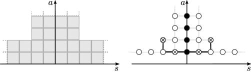
Figure 4: $\mathbb{T}$-shaped “fat hook” ($\mathbb{T}$-hook) uniting two ${\rm SU}(2|2)$ fat hooks, see [13] for this $\mathbb{T}$-hook and its generalization [35].

In the supersymmetric models the Hirota equation [13] appears to be a little more then the Y-system (2.15) in which two corner equations are missing. When one tries truncate the Y-system from the full $(a,s)$ plane lattice to the $\mathbb{T}$-hook one has to put $Y$-functions to zero on the vertical boundaries, and to $\infty$ at the horizontal boundaries in the left figure of Fig.4. Then the equation for $Y_{2,\pm 2}$ contains an uncertainty $\frac{0}{0}$. The Y-system has to be supplemented by additional information. In this respect, the T-system, free of that uncertainty, looks more fundamental than the Y-system.

To fix the functions $Y_{2,\pm 2}(u)$ at the corner nodes we will use a fact noticed from TBA [14, 15, 16] (and partially inspired by ): in the mirror kinematics, $Y_{2,\pm 2}(u)$ and $Y_{1,\pm 1}(u)$ are related on two sides of the cut $(-\infty,-2g)\cup(2g,\infty)$ on $\mathbb{R}$ by

$$Y_{2,\pm 2}(u+i0)=\frac{1}{Y_{1,\pm 1}(u-i0)}\,.$$ (5.3)

In the next section we will use (5.3) as a natural analytic input for the asymptotic large $L$ solution of the quantum Y-system.

Given a particular solution of the Y-system, the corresponding energy of a string state (or anomalous dimension of a SYM operator) can be obtained from

$$E=\sum_{j}\epsilon^{{\rm ph}}_{1}(u_{4,j})+\sum_{a=1}^{\infty}\int_{-\infty}^{\infty}\frac{du}{2\pi i}\,\,\frac{\partial\epsilon_{a}^{\rm mir}}{\partial u}\log\left(1+Y_{a,0}(u)\right),$$ (5.4)

whose general form is rather standard in the TBA context. The physical energy $\epsilon_{a}^{\rm ph}$ or the mirror momentum $\epsilon_{a}^{\rm mir}$ are defined by the same formula

$$\epsilon_{a}(u)=a+\frac{2ig}{x^{[+a]}}-\frac{2ig}{x^{[-a]}}\;.$$ (5.5)

with the corresponding choice of $x(u)$ from (5.2).

The physical roots $u_{4,j}$ are subject to the exact, finite size Bethe ansatz equations

$$Y^{\rm ph}_{1,0}(u_{4,j})=-1\,$$ (5.6)

where the $Y^{\rm ph}_{1,0}(u)$ was explicitly defined in [20] as an analytic continuation of $Y_{1,0}(u)$ down through the cut $(-\infty,-2g+\tfrac{i}{2})\cup(+2g+\tfrac{i}{2},+\infty)$. The first term in (5.4) is given by the logarithmic pole contributions from the second one at the points $u_{4,j}$.

It is also important to mention that at large $L$ the Y-functions of the middle (black) nodes are exponentially suppressed on the real axis in the mirror sheet

$$Y_{a,0}(u)\sim e^{-ip^{\rm mir}_{a}(u)L}\,,\qquad{\rm where}\quad p_{a}(u)=-i\log\left(\frac{x^{[+a]}}{x^{[-a]}}\right)^{L}\;.$$ (5.7)

5.1 Integrability of AdS/CFT Y-system and large volume limit

To study the AdS/CFT Y-system we need to clarify the analyticity properties of the Y-functions. Most of this information is due to the TBA derivation of the $Y$-system. The full understanding of these properties still needs additional efforts (see [37] for some advances). We will try to summarize them and demonstrate their naturalness. Ideal would be to postulate these properties from some simple and natural physical principles and then deduce from them the asymptotic Bethe ansatz (ABA) equations, along with the dressing factor (ignoring the standard S-matrix bootstrap procedure) as it can be done for various relativistic sigma-models (see [12, 38] for an inspiring example of the $SU(N)\times SU(N)$ principal chiral field). On our current level of understanding of the AdS/CFT Y-system, this program can be fulfilled only partially.

This Y-system is equivalent to Hirota eq.(2.7) in the $\mathbb{T}$-hook fig.4(left) with specific analyticity conditions. Fortunately, many of the results for the simplified Hirota eq.(4.1) for quasi-classical AdS/CFT, in particular (4.4) and (4.2), as well as the analyticity (4.7)-(4.10), can be generalized to the full quantum case. We will demonstrate in this section that the asymptotic Bethe ansatz (ABA) of [39] can be explained, and partially derived from the AdS/CFT Y-system (2.15) together with the relation (5.3), providing the reality of Y-functions, the $s\leftrightarrow-s$ symmetry and certain natural analyticity assumptions, such as the existence of analyticity strips in $u$-plane.

5.2 Generating functional for ${\rm U}(2,2|4)$ T-functions

Since Hirota equation for AdS₅/CFT₄ is exactly the same as the one considered in the Sec.2 for spin chains one may try to construct its general solution in terms of only a few functions. But we here we deal with a non-compact symmetry group, and the ${\mathbb{T}}$-hook instead of the usual ${\mathbb{L}}$-shaped fat hook domain for the Y-system as a consequence. In the pervious section, in the strong coupling limit the difference between the $U(4|4)$ and $U(2,2|4)$ generating functions was only in the way we expand various parts of (4.2) w.r.t. the generating parameter $t$. A natural generalization of (3.11) for the quantum case or the $\mathbb{T}$-hook gives $T_{1,s}(u)$ in terms of the generating functional [19]

$$W = \left[(1-D{\cal Y}_{1}D)\frac{1}{1-D{\cal X}_{1}D}\frac{1}{1-D{\cal X}_{2}D}(1-D{\cal Y}_{2}D)\right]_{+}\times$$

$$\left[(1-D{\cal Y}_{3}D)\frac{1}{1-D{\cal X}_{3}D}\frac{1}{1-D{\cal X}_{4}D}(1-D{\cal Y}_{4}D)\right]_{-}=\sum_{s=-\infty}^{\infty}D^{s}T_{1,s}D^{s}$$

Here $\{{\cal Y}_{1}(u)|{\cal X}_{1}(u),{\cal X}_{2}(u)|{\cal Y}_{2}(u),{\cal Y}_{3}(u)|{\cal X}_{3}(u),{\cal X}_{4}(u)|{\cal Y}_{4}(u)\}$ are 8 arbitrary functions of the spectral parameter $u$ parameterizing the general solution where, as a convenient choice for the AdS/CFT system, the grading is fixed by the Kac-Dynkin diagram $\bigotimes\!\!-\!\!\bigcirc\!\!-\!\!\bigotimes\!\!-\!\!\bigcirc\!\!-\!\!\bigotimes\!\!-\!\!\bigcirc\!\!-\!\!\bigotimes$. Similarly to the $U(2,2|4)$ characters (see after eq. (4.4)), we expand in positive powers of the shift operator $D$   (replacing the $t$ of (4.2)) inside the bracket $\left[\dots\right]_{+}$ corresponding to the $u(2|2)_{R}$ sub-algebra, and in negative powers of $D$ inside the bracket $\left[\dots\right]_{-}$ corresponding to the $u(2|2)_{L}$ subalgebra . As a result one gets an infinite sum for each $T_{1,s},\,\,\,-\infty<s<\infty$. Note also that (5.2) corresponds to a gauge where $T_{0,s}=1$ and all other $T_{a,s}$ can be found from (2.16).

In the asymptotic $L\to\infty$ limit the full Y-system in the $U(2,2|4)$ $\mathbb{T}$-hook almost splits into two Y-subsystems of two $su(2|2)_{L,R}$ fat hooks corresponding to the $L,R$ wings: ${\cal X}_{1},{\cal X}_{2},{\cal Y}_{1},{\cal Y}_{2}$ are exponentially small whereas ${\cal X}_{3},{\cal X}_{4},{\cal Y}_{3},{\cal Y}_{4}$ are exponentially large, thus the terms in the sum over $s$ are organized in powers of wrapping.

We can easily find these 8 functions in the $L\to\infty$ limit by comparing $T_{1,1}(u)$ generated from (5.2) with the explicit asymptotic solution of the Y-system with given Bethe roots found in [13] (partially by matching with the known ABA of [39])

$${\cal Y}_{1}=H_{R}F_{0}^{+}\frac{{\cal Q}_{1}^{-}}{{\cal Q}_{1}^{+}}\;\;,\;\;{\cal X}_{1}=H_{R}\frac{{\cal Q}_{1}^{-}{\cal Q}_{2}^{++}}{{\cal Q}_{1}^{+}{\cal Q}_{2}}\;\;,\;\;{\cal X}_{2}=H_{R}\frac{{\cal Q}_{2}^{--}{\cal Q}_{3}^{+}}{{\cal Q}_{2}{\cal Q}_{3}^{-}}\;\;,\;\;{\cal Y}_{2}=H_{R}\frac{{\cal Q}^{+}_{3}}{{\cal Q}_{3}^{-}}F_{4}^{-}\;,$$

$${\cal Y}_{4}=H_{L}\frac{1}{F_{0}^{-}}\frac{{\cal Q}_{7}^{+}}{{\cal Q}_{7}^{-}}\;\;,\;\;{\cal X}_{4}=H_{L}\frac{{\cal Q}_{7}^{+}{\cal Q}_{6}^{--}}{{\cal Q}_{7}^{-}{\cal Q}_{6}}\;\;,\;\;{\cal X}_{3}=H_{L}\frac{{\cal Q}_{6}^{++}{\cal Q}_{5}^{-}}{{\cal Q}_{6}{\cal Q}_{5}^{+}}\;\;,\;\;{\cal Y}_{3}=H_{L}\frac{{\cal Q}^{-}_{5}}{{\cal Q}_{5}^{+}}\frac{1}{F_{4}^{+}}\;$$ (5.9)

$${\rm where}\quad F_{4}=\prod_{j}\frac{x-x_{4,j}^{+}}{x-x_{4,j}^{-}}\;\;,\;\;H_{R}=\left(\frac{x^{-}}{x^{+}}\right)^{\tfrac{L}{2}}\prod_{j}\frac{x^{+}-x_{4,j}^{-}}{x^{-}-x_{4,j}^{-}}\sigma(u,x^{\pm}_{4,j})$$ (5.10)

$$F_{0}=\bar{F}_{4}\;\;,\;\;H_{L}=\tilde{H}_{R}\,.$$ (5.11)

As before, the bar means the complex conjugation in mirror plane whereas the tilde is the complex conjugation in physical plane. The ${\cal Q}_{a}$ functions generalize the Baxter polynomials - they are generic ”polynomials” on the two-sheet Riemann surface

$${\cal Q}_{a}=\prod_{j=1}^{K_{a}}(x(u)-y_{a,j})\prod_{j=1}^{\bar{K}_{a}}\left(\frac{1}{x(u)}-y_{\bar{a},j}\right)\;.$$ (5.12)

The roots of these polynomials are constrained by the mirror reality condition of the $Y$ functions. Namely, we have, as in the strong coupling limit (4.9)

$$\overline{{\cal X}_{1}}={\cal X}_{2}\;\;,\;\;\overline{{\cal Y}_{1}}={\cal Y}_{2}\;.$$ (5.13)

This asymptotic solution has a few important symmetries and analytic properties. We will study some of them below. It is very important to find a minimal set of such properties, such as reality and analyticity, which can be used then to constrain the $8$ functions parameterizing the general solution, to generate only the physically relevant solutions. We present below a possible list of some of such properties which, in our opinion, should be satisfied by the physical solutions and try to constrain by them the ABA solution (5.2). This program worked well for the principal chiral field model [12, 38] but it appears to be more tricky to do it for the AdS/CFT Y-system.

We will show that an essential part of ABA can be derived from these properties.

5.3 Minimal analyticity structure of Y-functions

Here we summarize some of the analyticity properties of Y-functions which, by our assumption, are satisfied by the physical solutions of the AdS/CFT Y-system:
 Reality:

1. Reality of Y-functions $\bar{Y}_{a,s}=Y_{a,s}$

2. Reality of the Bethe roots $u_{4,j}$

Analyticity:

1. $Y_{1,\pm 1},\;Y_{2,\pm 2}$ should have a Zhukovski cut on the real axes and be related by (5.3)

2. $Y_{1,s}$ should have no branch cuts inside the strip $-\tfrac{s-1}{2}<{\rm Im}\,u<\tfrac{s-1}{2}$

3. $Y_{a,1}$ should have no branch cuts inside the strip $-\tfrac{a-1}{2}<{\rm Im}\,u<\tfrac{a-1}{2}$

4. $Y_{a,0}$ should have no branch cuts inside the strip $-\tfrac{a}{2}<{\rm Im}\,u<\tfrac{a}{2}$

This list may be not enough to completely constrain the ABA and the physical meaning of some of them remains to be understood. All this deserves an additional study. But these properties are consistent with the TBA equations for the excited states.

In what follows we consider for simplicity the operators/states obeying the symmetry $Y_{a,s}=Y_{a,-s}$. The generalization to the full asymmetric case is almost straightforward. One can see that $Y_{a,s}=Y_{a,-s}$ implies (which is also true for finite $L$)

$$\frac{{\cal X}_{4}^{+}}{{\cal Y}_{4}^{+}}=\frac{{\cal Y}_{1}^{-}}{{\cal X}_{1}^{-}}\;\;,\;\;\frac{{\cal X}_{4}}{{\cal X}_{3}}=\frac{{\cal X}_{2}}{{\cal X}_{1}}\;\;,\;\;\frac{{\cal X}_{3}^{-}}{{\cal Y}_{3}^{-}}=\frac{{\cal Y}_{2}^{+}}{{\cal X}_{2}^{+}}\;.$$ (5.14)

5.3.1 Reality

Reality of $Y_{a,s>0}$ implies that $T_{a,s}$ are also real up to a gauge transformation. Here we will examine this condition in the asymptotic large $L$ limit.

It is easy to see that since the first four functions ${\cal X}_{1},{\cal Y}_{1},{\cal Y}_{2},{\cal X}_{2}$ are small whereas ${\cal X}_{3},{\cal Y}_{3},{\cal Y}_{4},{\cal X}_{4}$ are large in the $L\to\infty$ limit only a half of the generating functional (5.2) (corresponding to one of the subgroups $su(2|2)_{L,R}$) contributes. For $s\geq 0$ the full functional reduces to [40]

$${\cal W}^{R}\simeq(1-D{\cal Y}_{1}D)\frac{1}{1-D{\cal X}_{1}D}\frac{1}{1-D{\cal X}_{2}D}(1-D{\cal Y}_{2}D)\frac{{\cal Y}_{3}^{-}{\cal Y}_{4}^{+}}{{\cal X}_{3}^{-}{\cal X}_{4}^{+}}=\sum_{s=0}^{\infty}D^{s}T_{1,s}D^{s}$$ (5.15)

Since we fixed $T_{0,s}=1$ we have only two degrees of freedom left: one is a possible redefinition of $D\to g(u)D$ which does not change the definition of the shift operator, whereas another corresponds to the transformation is ${\cal W}\to{\cal W}g(u)$. In particular, we can remove the last factor from (5.15) by a desired gauge transformation (2.13) to get

$${\cal W}=(1-D{\cal Y}_{1}D)\frac{1}{1-D{\cal X}_{1}D}\frac{1}{1-D{\cal X}_{2}D}(1-D{\cal Y}_{2}D)\;.$$ (5.16)

Let us show that the hermiticity of the above generating functional automatically implies the reality of all $Y_{a,s>0}$. Indeed since $D$ is hermitian we have

$${\cal W} = \sum_{s}D^{s}T_{1,s}D^{s}=\sum_{s}D^{s}\bar{T}_{1,s}D^{s}={\cal W}^{\dagger}$$

$$= (1-D\bar{\cal Y}_{2}D)\frac{1}{1-D\bar{\cal X}_{2}D}\frac{1}{1-D\bar{\cal X}_{1}D}(1-D\bar{\cal Y}_{1}D)\;,$$

which is equivalent to (5.13): since we have to equate the coefficients of infinitely many powers of $D$ the monomials should coincide. This relation is a quantum analog of (4.8). Notice that (5.13) implies (assuming that $H_{R}$ and $F_{4}$ do not depend explicitly on the Bethe roots $y_{a,j},y_{\bar{a},j}$) that

$$\bar{\cal Q}_{1}={\cal Q}_{3}\;,\quad\bar{\cal Q}_{2}={\cal Q}_{2}\;,\quad{\bar{F}_{4}}={F_{0}}\;,\quad{\bar{H}_{R}}={H_{R}}\;.$$ (5.18)

The first equality implies that $y_{\bar{1},j}=y_{3,j},\;y_{1,j}=y_{\bar{3},j}$. The second equality tells us that $y_{2,j}=y_{\bar{2},j}$ i.e. that ${\cal Q}_{2}$ is a usual polynomial of $u$. Notice that the combination ${\cal Q}_{1}{\cal Q}_{3}$ is a polynomial of $u$. Finally, the last equality implies for the (unitary) dressing factor

$$\prod_{j}\frac{\sigma(u,u_{4,j})}{\bar{\sigma}(u,u_{4,j})}=\prod_{j}\frac{1/x^{-}-x_{4,j}^{+}}{1/x^{+}-x_{4,j}^{+}}\frac{x^{-}-x_{4,j}^{-}}{x^{+}-x_{4,j}^{-}}\;$$ (5.19)

which is the crossing condition of [41]! (see [42] for its solution).

5.3.2 Analyticity properties 1), 2)

To see the consequences of the analyticity property 1) let us make a simple observation. By a direct calculation of the corresponding T-functions from (5.16) we get

$$Y_{1,+1}Y_{2,+2}\simeq\frac{{\cal X}_{1}^{-}{\cal X}_{2}^{+}}{{\cal Y}_{1}^{-}{\cal Y}_{2}^{+}}=\frac{1}{F_{0}F_{4}}\;,$$ (5.20)

and hence the property 1) immediately implies $F_{0}(u+i0)F_{4}(u+i0)=\frac{1}{F_{0}(u-i0)F_{4}(u-i0)}\;.$ To arrive to the above conclusion we used a weaker version of the property 1) for the product of two $Y$ functions. In fact, one can get more from the property 1), namely $F_{4}^{[+0]}=1/F_{0}^{[-0]}\;$, which together with (5.18) gives a powerful constraint on the functions $F_{4}$ and $F_{0}$. We will show below that requiring $F_{4}$ and $F_{0}$ to have only one Zhukovski cut on the real axes leads to the conditions 2) and 3).

Let us study the property 2). Notice that the transformation ${\cal X}_{1,2}\to g{\cal X}_{1,2},\;{\cal Y}_{1,2}\to\;g{\cal Y}_{1,2}$ where $g(u)$ is an arbitrary function, does not affect $Y_{1,s}$ and therefore it is a gauge transformation. If we take $g=\frac{{\cal Q}^{+}_{1}}{H_{R}{\cal Q}_{1}^{-}}$ we notice that ${\cal Q}_{1}$ appears only in the combination ${\cal Q}_{1}{\cal Q}_{3}$, which does not have branch cuts as we have shown above. This implies that in that gauge ${\cal X}_{1}$ and ${\cal X}_{2}$ have no branch cuts any more. Expanding the denominator in (5.16) we get
$W\simeq\sum\limits_{s=0}^{\infty}D^{s}(1-D{\cal Y}_{1}^{[+s]}D)\left(\sum_{n=-s}^{s}{\cal X}_{1}^{[-s+1]}\dots\cal X_{1}^{[n-1]}{\cal X}_{2}^{[n+1]}\dots\cal X_{2}^{[+s-1]}\right)(1-D{\cal Y}_{2}^{[-s]}D)D^{s}.$ The cuts in $T_{1,s}$ come only from ${\cal Y}_{1}^{[+s-1]}$ and ${\cal Y}_{2}^{[-s+1]}$. The analyticity requirement 2) is satisfied since $T_{1,s}\sim{\cal Y}_{1}^{[+s-1]}{\cal Y}_{2}^{[-s+1]}\sim F_{0}^{[+s]}F_{4}^{[-s]}$ have the analyticity strip $|{\rm Im}\,(u)|<s/2$ because $F_{0},F_{4}$ have only a single cut one the real axes.

5.3.3 Duality transformation and analyticity 3)

Similarly to the Sec.3.5 we can consider a duality transformation as an effect of the commutation of two operatorial factors within the generating functional:

$$(1-D{\cal X}_{1}D)^{-1}(1-D{\cal Y}_{1}D)=(1-D\hat{\cal Y}_{1}D)(1-D\hat{\cal X}_{1}D)^{-1}$$ (5.21)

and a similar equation for the factors with ${\cal X}_{2},{\cal Y}_{2}$. It is convenient to parameterize the new factors as (compare it with (3.6),(3.18))

$$\hat{\cal X}_{1}=\hat{H}_{R}\frac{\hat{\cal Q}_{1}^{+}}{\hat{\cal Q}_{1}^{-}}\frac{1}{F_{0}^{-}}\;\;,\;\;\hat{\cal Y}_{1}=\hat{H}_{R}\frac{{\cal Q}_{2}^{--}\hat{\cal Q}_{1}^{+}}{{\cal Q}_{2}\hat{\cal Q}_{1}^{-}}\;\;,\;\;\hat{\cal Y}_{2}=\hat{H}_{R}\frac{{\cal Q}_{2}^{++}\hat{\cal Q}_{3}^{-}}{{\cal Q}_{2}\hat{\cal Q}_{3}^{+}}\;\;,\;\;\hat{\cal X}_{2}=\hat{H}_{R}\frac{\hat{\cal Q}_{3}^{-}}{\hat{\cal Q}_{3}^{+}}\frac{1}{F_{4}^{+}}$$ (5.22)

where by definition $\hat{H}_{R}$ can only depend on the momentum carrying roots $u_{4,k}$ whereas $\hat{Q}_{1}$ is a function of the form (5.12). In this parameterization we have $\hat{\cal X}_{1}^{+}/\hat{\cal Y}_{1}^{+}={\cal X}_{1}^{-}/{\cal Y}_{1}^{-},\;\hat{\cal X}_{2}^{-}/\hat{\cal Y}_{2}^{-}={\cal X}_{2}^{+}/{\cal Y}_{2}^{+}$ and to keep (5.16) intact we only have to satisfy commpare with (3.19)) $\hat{\cal X}_{1}-\hat{\cal Y}_{1}={\cal X}_{1}-{\cal Y}_{1}\;\;,\;\;\hat{\cal X}_{2}-\hat{\cal Y}_{2}={\cal X}_{2}-{\cal Y}_{2}$ Second equation is the complex conjugate of the first one. The first equation gives $\frac{\hat{\cal Q}_{1}^{+}{\cal Q}_{1}^{+}}{\hat{\cal Q}_{1}^{-}{\cal Q}_{1}^{-}}=F_{0}^{-}\frac{H_{R}}{\hat{H}_{R}}\,\,\,\frac{F_{0}^{+}{\cal Q}_{2}-{{\cal Q}_{2}^{++}}}{F_{0}^{-}{\cal Q}_{2}^{--}-{\cal Q}_{2}}$ which has the solution $\hat{\cal Q}_{1}{\cal Q}_{1}=f(u,x_{4,k})(F_{0}{\cal Q}_{2}^{-}-{\cal Q}_{2}^{+})\,.$ Since the r.h.s. has no poles at $x=1/x_{4,k}^{+}$ and cannot explicitly depend on $x_{4,k}$ we should take $f=C\,\prod_{k}(1/x-x_{4,k}^{+})$ to cancel the poles in $F_{0}$. This leads to the condition $\hat{\cal Q}_{1}{\cal Q}_{1}\propto{\cal Q}_{2}^{+}\prod_{k=1}^{K_{4}}(1/x-x_{4,k}^{+})-{{\cal Q}_{2}^{-}}\prod_{k=1}^{K_{4}}(1/x-x_{4,k}^{-})$ from where we can determine $\hat{\cal Q}_{1}$ and its complex conjugate $\hat{\cal Q}_{3}$. The resulting formulas are analogous to (3.20).

We demonstrated above that the terms in the generating functional can be reshuffled in such a way that the expression for the new elementary factors (5.22) are very similar to the initial ones (5.2), with the modified Bethe roots.

Now let us use this fact to show that $Y_{a,1}$ are also analytic in their strips given in the property 3). Indeed, using the Bäcklund relations, in the way similar to the subsection 3.3 where $T_{a,s}$ was generated from ${\cal W},$ we can show that $T_{a,1}$ can be computed from ${\cal W}^{-1}$ as follows [9]

$${\cal W}^{-1}=(1-D\hat{\cal X}_{2}D)\frac{1}{1-D\hat{\cal Y}_{2}D}\frac{1}{1-D\hat{\cal Y}_{1}D}(1-D\hat{\cal X}_{1}D)\simeq\sum_{a=0}^{\infty}(-1)^{a}D^{a}T_{a,1}D^{a}\;.$$ (5.23)

As we saw in subsection 5.3.2, for the analyticity of T-functions in their physical strips $F_{4}$ should have a cut only on the real axes. The arguments given there can be also applied to the functional (5.23) which leads to the proof of the property 3). It also shows that in a certain gauge $T_{a,1}$ has the analyticity strip $|{\rm Im}\,(u)|<a/2$.

Due to (5.7) we can drop the denominator in the r.h.s. of (2.15) at $s=0$ and rewrite it, using $1+Y_{a,s}=\frac{T_{a,s}^{+}T_{a,s}^{-}}{T_{a+1,s}T_{a-1,s}}$ following from (2.7) and (2.14), $\frac{Y_{a,0}^{+}Y_{a,0}^{-}}{Y_{a-1,0}Y_{a+1,0}}\simeq\left(\frac{T_{a,1}^{+}T_{a,1}^{-}}{T_{a-1,1}T_{a+1,1}}\right)^{2}\,,$ where in the equation for $a=1$ one should replace in the l.h.s. $Y_{0,0}$ by $1.$ Solving this Y-system equation for $Y_{a,0}$ we get $Y_{a,0}=\frac{\phi(u+ia/2)}{\phi(u-ia/2)}T_{a,1}^{2}$ where the first factor, a zero mode, is easy to calculate since $\phi(u)$ can be extracted from $Y_{1,0}$. Hence the most complicated part of $Y_{a,0}$ is hidden in $T_{a,1}$ and has the correct analyticity structure 4). The proof of the correct analyticity of the factor $\frac{\phi(u+ia/2)}{\phi(u-ia/2)}$ is left to the reader.

5.3.4 Reality of $Y_{a,0}$

Finally let us also imply the reality condition to $Y_{1,0}=\frac{({\cal Y}_{1}-{\cal X}_{1}-{\cal X}_{2}+{\cal Y}_{2})^{2}}{{\cal Y}_{2}{\cal Y}_{3}}$. Note that the numerator is real, so for the reality of $Y_{1,0}$ we only have to require that ${\cal Y}_{2}{\cal Y}_{3}=H_{L}H_{R}\frac{F_{4}^{-}}{F_{4}^{+}}$ is real. Note that the factors $H_{R}$ is a real function as a consequence of the crossing equation in the mirror kinematics stemming from the last of eqs.(5.18). In the physical kinematics $H_{L}$ is conjugate to $H_{R}$ and naively one would expect it to be also real as well. However the conjugation in the physical sense does not necessarily commute with the mirror conjugation. Explicit calculation shows that ${\cal Y}_{2}{\cal Y}_{3}=\frac{Q_{4}^{++}Q_{4}^{--}}{Q_{4}^{2}}\;\;,\;\;Q_{4}=\prod_{k=1}^{K_{4}}(u-u_{4,k})$ which is indeed real. The reality of all other $Y_{a,0}$ follows from the Y-system.

Finally, the above expression for $Y_{1,0}$ simplifies on a Bethe root $u=u_{4,k}$: since $1/F_{4}^{-}(u_{4,k})=0~{}$, ${\cal Y}_{2}$ dominates the numerator and we get from $Y_{1,0}(u_{4,k})={\cal Y}_{2}/{\cal Y}_{3}=\frac{H_{R}}{H_{L}}F_{4}^{+}F_{4}^{-}\frac{{\cal Q}_{3}^{+}{\cal Q}_{5}^{+}}{{\cal Q}_{3}^{-}{\cal Q}_{5}^{-}}=-1$. Since $H_{R}$ is a complex conjugate of $H_{L}$ we see that $Y_{1,0}(u_{4,k})$ is unimodular in the physical kinematics, ensuring the reality of the Bethe roots $u_{4,k}$.

6 Conclusions and perspectives

Our main purpose in these notes was mainly pedagogical: to show the power of Hirota discrete integrable dynamics (HDID) for the solution of quantum integrable models. The Bäcklund method of solution of Hirota equation for fusion in the supersymmetric generalizations of the Heisenberg spin chain, with the polynomiality condition of the transfer matrix gives a rather direct way of derivation of the final Bethe ansatz equations for the roots of Baxter’s Q-polynomials. However, the applications of HDID is not limited to the spin chains and can be quite efficient in the study of integrable CFT’s, $\sigma$-models at finite volume and, remarkably, in such a complicated problem as the AdS₅/CFT₄ system.

We demonstrated that the general asymptotic solution of Y-system for AdS/CFT obeys several remarkable analyticity and reality properties. They seem to be rather constraining and could be used at finite volume to single out the physically relevant solutions of this Y-system. It seems possible to reverse the logic and derive the asymptotic Bethe ansatz equations from these equations, as in relativistic $\sigma$-models.

We hope that further study of this circle of questions, and in particular of the role and the consequences of the equation (5.3), will lead to the complete understanding of the analyticity structure of the integrable AdS/CFT systems. This understanding, together with the solutions of Y-system stemming from the HDID (in the form the generating functional (5.2) or in the Wronskian form recently obtained in [43]) should allow to reduce the problem to a finite set of integral Destri-DeVega type equations.

Acknowledgments

The work of VK was partly supported by the ANR grants INT-AdS/CFT
(ANR36ADSCSTZ) and GranMA (BLAN-08-1-313695) and the grant RFFI 08-02-00287. V.K. also thanks NORDITA institute in Stokholm, as well as Vladimir Bazhanov and the theoretical physics group of Australian National University (Canberra) for the kind hospitality and interesting discussions. We thank Sebastien Leurent, Zengo Tsuboi, Pedro Vieira and especially Dymitro Volin for useful discussions.

References

- [1] R. Hirota, Journal of the Phys. Soc. of Japan, 50 (1981) 3785-3791.
- [2] M. Jimbo and T. Miwa, Publ. Res. Inst. Math. Sci. Kyoto 19 (1983) 943.
- [3] A. Klümper and P. A. Pearce, Physica A 183 (1992) 304. ; A. Kuniba, T. Nakanishi and J. Suzuki, Int. J. Mod. Phys. A 9 (1994) 5215 ; L. Faddeev, A. Volkov, Lett. Math. Phys. 32 (1994) 125
- [4] Al. B. Zamolodchikov, Nuclear Physics B 342, (1990) 695
- [5] V. V. Bazhanov, S. L. Lukyanov and A. B. Zamolodchikov, Commun. Math. Phys. 177 (1996) 381
- [6] I. Krichever, O. Lipan, P. Wiegmann and A. Zabrodin, Commun. Math. Phys. 188 (1997) 267
- [7] V. V. Bazhanov, S. L. Lukyanov and A. B. Zamolodchikov, Nucl. Phys. B 489, 487 (1997) ; P. Dorey and R. Tateo, Nucl. Phys. B 482, 639 (1996) ; G. Juttner, A. Klumper and J. Suzuki, Nucl. Phys. B 512 (1998) 581 ; P. Fendley, Nucl. Phys. B 374, 667 (1992) ; D. Fioravanti, A. Mariottini, E. Quattrini and F. Ravanini, Phys. Lett. B 390 (1997) 243 [arXiv:hep-th/9608091].
- [8] Z. Tsuboi, J. Phys. A 30, 7975 (1997) ; Z. Tsuboi, Physica A 252, 565 (1998)
- [9] V. Kazakov, A. S. Sorin and A. Zabrodin, Nucl. Phys. B 790 (2008) 345
- [10] V. Kazakov and P. Vieira, JHEP 0810 (2008) 050 ; V. Kazakov, S. Leurent, Z. Tsuboi, [arXiv:1010.4022 [math-ph]].
- [11] V. V. Bazhanov and Z. Tsuboi, Nucl. Phys. B 805 (2008) 451 ; Z. Tsuboi, Nucl.Phys.B 826 (2010) 399
- [12] N. Gromov, V. Kazakov and P. Vieira, JHEP 0912 (2009) 060
- [13] N. Gromov, V. Kazakov and P. Vieira, Phys. Rev. Lett. 103 (2009) 131601
- [14] D. Bombardelli, D. Fioravanti and R. Tateo, J. Phys. A 42, 375401 (2009)
- [15] N. Gromov, V. Kazakov, A. Kozak and P. Vieira, Lett. Math. Phys. 91(2010)265
- [16] G. Arutyunov and S. Frolov, JHEP 0905 (2009) 068
- [17] R. A. Janik and T. Lukowski, Phys. Rev. D 76, 126008 (2007) ; M. P. Heller, R. A. Janik and T. Lukowski, JHEP 0806, 036 (2008) ; Z. Bajnok and R. A. Janik, Nucl. Phys. B 807, 625 (2009) ; Z. Bajnok, R. A. Janik and T. Lukowski, arXiv:0811.4448 [hep-th]. ; F. Fiamberti, A. Santambrogio, C. Sieg and D. Zanon, Nucl. Phys. B 805 (2008) 231 ; V. N. Velizhanin, arXiv:0811.0607 [hep-th] ; G. Arutyunov, S. Frolov and R. Suzuki, arXiv:1002.1711 [hep-th]. ; T. Lukowski, A. Rej and V. N. Velizhanin, Nucl. Phys. B 831 (2010) 105 ; J. Balog and A. Hegedus, JHEP 1006, 080 (2010) ; V. N. Velizhanin, arXiv:0811.0607 [hep-th].
- [18] N. Gromov, JHEP 1001, 112 (2010)
- [19] N. Gromov, V. Kazakov and Z. Tsuboi, JHEP 07 (2010) 097
- [20] N. Gromov, V. Kazakov, P. Vieira, Phys. Rev. Lett. 104 (2010) 211601. [arXiv:0906.4240 [hep-th]].
- [21] Z.Bajnok, “Review of AdS/CFT Integrability, Chapter III.6: Thermodynamic Bethe Ansatz,” arXiv:1012.3995 [hep-th].
- [22] S. S. Gubser, I. R. Klebanov and A. M. Polyakov, Phys. Lett. B 428 (1998) 105
- [23] A. Zabrodin, arXiv:0705.4006 [hep-th].
- [24] L. D. Faddeev, arXiv:hep-th/9605187.
- [25] V. V. Bazhanov and N. Y. Reshetikhin, Int. J. Mod. Phys. A 4 (1989) 115.
- [26] I. Bena, J. Polchinski and R. Roiban, Phys. Rev. D 69, 046002 (2004)
- [27] N. Beisert, V. Kazakov, K. Sakai, K. Zarembo, Comm.Math.Phys. 263, 659 (2006)
- [28] S.Schäfer-Nameki, “Review of AdS/CFT Integrability, Chapter II.4: The Spectral Curve,” arXiv:1012.3989 [hep-th].
- [29] S.-J. Cheng, N. Lam and R.B. Zhang, J. Algebra 273, 780 (2004)
- [30] J.-H. Kwon, Adv. Math. 217 713 (2008)
- [31] D. Serban and M. Staudacher, JHEP 0406 (2004) 001
- [32] N. Beisert, V. A. Kazakov, K. Sakai and K. Zarembo, JHEP 0507 (2005) 030
- [33] G. Japaridze, A. Nersesian and P.Wiegmann, Nucl. Phys. B 230 (1984) 511. ; E. Ogievetsky and P. Wiegmann, Phys. Lett. B 168 (1986) 360. ; E. Ogievetsky, P. Wiegmann and N. Reshetikhin, Nucl. Phys. B 280 (1987) 45.
- [34] N. Dorey and B. Vicedo, JHEP 0703, 045 (2007)
- [35] A. Hegedus, Nucl. Phys. B 825, 341 (2010)
- [36] N. Gromov and P. Vieira, Nucl. Phys. B 789 (2008) 175
- [37] A. Cavaglia, D. Fioravanti and R. Tateo, arXiv:1005.3016 [hep-th].
- [38] V. Kazakov and S. Leurent, arXiv:1007.1770 [hep-th].
- [39] N. Beisert, B. Eden and M. Staudacher, J. Stat. Mech. 0701 (2007) P021
- [40] N. Beisert, J. Stat. Mech. 0701, P017 (2007)
- [41] R. A. Janik, Phys. Rev. D73 (2006) 086006
- [42] P.Vieira and D.Volin, “Review of AdS/CFT Integrability, Chapter III.3: The Dressing Factor,” arXiv:1012.3992 [hep-th].
- [43] N. Gromov, V. Kazakov, S. Leurent, Z. Tsuboi [arXiv:1010.2720 [hep-th]].