Conserved quantities and generalized solutions of the ultradiscrete KdV equation

Abstract

We construct generalized solutions to the ultradiscrete KdV equation, including the so-called negative solition solutions. The method is based on the ultradiscretization of soliton solutions to the discrete KdV equation with gauge transformation. The conserved quantities of the ultradiscrete KdV equation are shown to be constructed in a similar way to those for the box-ball system.

1 Introduction

The ultradiscrete KdV equation:

$$U_{n}^{t+1}=\min\left[1-U_{n}^{t},\sum_{k=-\infty}^{n-1}\left(U_{k}^{t}-U_{k}^{t+1}\right)\right]$$ (1)

was first introduced as a dynamical equation for the so-called box-ball system (BBS)[1, 2]. Since (1) is closed on the binary values $0$ or $1$, if we regard $U_{n}^{t}$ as the number of balls in the $n$th box at time step $t$, and assume the boundary condition $\displaystyle\lim_{|n|\to\infty}U_{n}^{t}=0$, it describes the time evolution of balls in a one dimensional array of boxes. The updating rule of the BBS according to (1) can be expressed as follows. (See figure 1.)

• Find all the pairs of a ball and an adjacent vacant box to the right of it, and draw arclines from the ball to the vacant box for each of these pairs.

• Neglecting the pairs connected by arclines, find all the pairs of a ball and an adjacent vacant box to the right of it and draw arclines in a similar way.

• Repeat the above procedure until all the balls are connected to vacant boxes, then move all the balls into the vacant boxes connected by arclines.

An example of the time evolution pattern is shown in figure 2. The consecutive balls behave like solitons in the KdV equation. Furthermore, when we denote by $q_{1}$ the number of arclines drawn in the first step of the updating rule, by $q_{2}$ one in the second step and so on, we obtain a nonincreasing integer sequence $(q_{1},q_{2},q_{3},\ldots)$, which is a conserved quantity of the BBS in time[3].

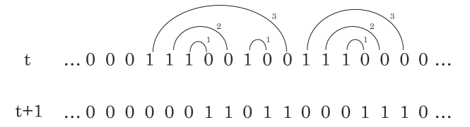
Figure 1: The update rules of the BBS. A vacant box and a box with a ball are represented by ‘0’ and ‘1’, respectively. The conserved quantities are simultaneously determined. ($q_{1}=3,\ q_{2}=q_{3}=2$.)

Figure 2: A solitonic time evolution pattern of the BBS. The symbol ‘.’ denotes ‘0’.

The reason why the BBS has these solitonic properties is understood by the fact that (1) is obtained from the KdV equation through a limiting procedure, ultradiscretization[4]. The process involved in obtaining (1) from the KdV equation can be explained as follows. The integrable discrete KdV equation is given in the bilinear form as

$$(1+\delta)\sigma_{n+1}^{t+1}\sigma_{n}^{t-1}=\delta\sigma_{n+1}^{t-1}\sigma_{n}^{t+1}+\sigma_{n}^{t}\sigma_{n+1}^{t},$$ (2)

where $(n,t)\in{\mathbb{Z}}^{2}$ and $\delta$ is a discretization parameter[5]. By putting

$$u_{n}^{t}:=\frac{\sigma_{n}^{t}\sigma_{n+1}^{t-1}}{\sigma_{n+1}^{t}\sigma_{n}^{t-1}},\quad v_{n}^{t}:=\frac{\sigma_{n}^{t+1}\sigma_{n}^{t-1}}{(\sigma_{n}^{t})^{2}},$$ (3)

(2) gives the simultaneous equations

$$(1+\delta)\frac{1}{u_{n}^{t+1}} =\delta u_{n}^{t}+\frac{1}{v_{n}^{t}},$$ (4)

$$u_{n}^{t+1}v_{n+1}^{t} =u_{n}^{t}v_{n}^{t}.$$ (5)

When we impose the boundary condition $\displaystyle\lim_{|n|\to\infty}\sigma_{n}^{t}=\mbox{const.}$, then $\displaystyle\lim_{|n|\to\infty}v_{n}^{t}=\lim_{|n|\to\infty}u_{n}^{t}=1$ from (4) and (5) we have

$$(1+\delta)\frac{1}{u_{n}^{t+1}}=\delta u_{n}^{t}+\prod_{k=-\infty}^{n-1}\frac{u_{k}^{t+1}}{u_{k}^{t}}.$$ (6)

We introduce a parameter $\epsilon$ and put $\displaystyle\delta:=e^{-1/\epsilon}$. If there exists a one parameter family of solutions to (6) $\displaystyle u_{n}^{t}(\epsilon)$, and if the limit $\displaystyle\lim_{\epsilon\to+0}\epsilon\log u_{n}^{t}(\epsilon)=:U_{n}^{t}$ exists, then, using the identities for arbitrary real numbers $a$ and $b$

$$\lim_{\epsilon\to+0}\epsilon\log\left(e^{a/\epsilon}+e^{b/\epsilon}\right)=\max[a,b],$$

$$\lim_{\epsilon\to+0}\epsilon\log\left(e^{a/\epsilon}\cdot e^{b/\epsilon}\right)=a+b,$$

$$-\max[-a,-b]=\min[a,b],$$

we find that $U_{n}^{t}$ satisfies (1).

Recently, (1) has been studied without the constraint of binary values[6, 7]. One interesting feature in this extension is that there exist background solutions composed of so-called negative solitons travelling at speed one[6]. A typical example of the background solutions is shown in figure 3. Furthermore, such negative solitons interact nontrivially with ordinary solitons as shown in figure 4. A method to solve the initial value problem for this generalized situation is given in Ref.[7]. From these properties, the dynamical systems described by (1) in the general setting are also regarded as integrable cellular automata, just as the BBS. However, several important features of integrable cellular automata have not been clarified yet, such as the conserved quantities, the relation to integrable lattice models, extension to the case of a cyclic boundary condition and so on, all of which are well understood in the case of BBS. In this article, we report that a simple transformation reveals the underlying integrable structure of (1) for the generalized states. By this transformation, the relation to the BBS and hence to the integrable lattice models, and generalization to a different boundary condition become apparent. We explicitly show how to obtain the conserved quantities and give the expression of general solutions to (1) where negative solitons and ordinary solitons coexist.

Figure 3: A time evolution pattern of a background solution.

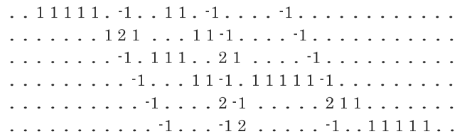
Figure 4: A time evolution pattern in which negative solitons and ordinary solitons coexist.

2 Conserved quantities for states with negative solitons

We start from the ultradiscretization of the coupled equations (4) and (5). By putting $\displaystyle\delta=e^{-1/\epsilon}$ and assuming that the limit

$$\lim_{\epsilon\to+0}\epsilon\log u_{n}^{t}(\epsilon)=:U_{n}^{t},\ \lim_{\epsilon\to+0}\epsilon\log v_{n}^{t}(\epsilon)=:V_{n}^{t}$$

exist, we obtain the equations

$$U_{n}^{t+1} =\min\left[1-U_{n}^{t},V_{n}^{t}\right],$$ (7)

$$V_{n+1}^{t} =U_{n}^{t}+V_{n}^{t}-U_{n}^{t+1}.$$ (8)

If we impose the boundary condition $\displaystyle\lim_{|n|\to\infty}U_{n}^{t}=\lim_{|n|\to\infty}V_{n}^{t}=0$, Eqs. (7) and (8) are equivalent to (1). It is easily seen that (7) and (8) are generalized by introducing a positive integer constants $L$ and $C$ as

$$U_{n}^{t+1} =U_{n}^{t}+\min\left[L-U_{n}^{t},V_{n}^{t}\right]-\min\left[U_{n}^{t},C-V_{n}^{t}\right],$$ (9)

$$V_{n+1}^{t} =U_{n}^{t}+V_{n}^{t}-U_{n}^{t+1}.$$ (10)

Equations (9) and (10) are known as the ultradiscrete limit of the modified KdV equation and are interpreted as a BBS of box capacity $L$ with carrier of capacity $C$ [8, 9]. At the same time, they represent the action of the combinatorial R-matrix of an $A_{1}^{(1)}$ crystal on a certain symmetric tensor product representation as long as $U_{n}^{t}\in\{0,1,\cdots,L\}$ and $V_{n}^{t}\in\{0,1,2,\cdots,C\}$[10]. Note that Eqs. (9) and (10) are closed under the values $U_{n}^{t}\in\{0,1,\cdots,L\}$ and $V_{n}^{t}\in\{0,1,2,\cdots,C\}$. Hence the time evolution patterns of the BBS are regarded as the ground states of a 2 dimensional integrable lattice model at temperature 0 and its generalization has been investigated in detail[11, 12].

When we allow $U_{n}^{t}$ or $V_{n}^{t}$ in (7) and (8) to take negative integer values and/or the values greater than $L$ or $C$ respectively, they are no longer interpreted as a BBS nor as a realization of the combinatorial R-matrix. For an arbitrary initial state including negative integer values, let $\displaystyle M:=-\min_{n\in{\mathbb{Z}}}\left[U_{n}^{0},V_{n}^{0},L-U_{n}^{0},C-V_{n}^{0}\right]$. When we change variables $\tilde{U}_{n}^{t}:=U_{n}^{t}+M,\ \tilde{V}_{n}^{t}:=V_{n}^{t}+M,\ \tilde{L}:=L+2M,\ \tilde{C}:=C+2M$, then we find that Eqs. (9) and (10) are unchanged under this gauge transformation[13], that is,

$$\tilde{U}_{n}^{t+1} =\tilde{U}_{n}^{t}+\min\left[\tilde{L}-\tilde{U}_{n}^{t},\tilde{V}_{n}^{t}\right]-\min\left[\tilde{U}_{n}^{t},\tilde{C}-\tilde{V}_{n}^{t}\right],$$

$$\tilde{V}_{n+1}^{t} =\tilde{U}_{n}^{t}+\tilde{V}_{n}^{t}-\tilde{U}_{n}^{t+1}.$$

Since these equations are closed under the values $\tilde{U}_{n}^{t}\in\{0,1,\cdots,L+2M\}$ and $\tilde{V}_{n}^{t}\in\{0,1,2,\cdots,C+2M\}$, and initial values $\tilde{U}_{n}^{0},\ \tilde{V}_{n}^{0}$ belong to the same sets, we can regard them as equations for a BBS with box capacity $L+2M$ and carrier capacity $C+2M$, and regard them as a realization of $A_{1}^{(1)}$ crystal lattice composed of a larger tensor product representation. Thus we can conclude that Eqs. (9) and (10) as well as Eqs. (7) and (8) do not change their mathematical structure even in the case where the dependent variable take negative integer values.

From the above argument, we find that we can identify the ultradiscrete KdV equation (1) as a BBS with larger box capacity when its dependent variables take negative integer values. The conserved quantities of the BBS have been widely investigated in general cases and we can apply the results to this system[11, 14]. In [11, 15], it is shown that the energy functions which are combinatorially determined, are conserved in time, and in [14] the path description for the conserved quantities is given. Here we give another expression of the conserved quantities for (1).

Let $\displaystyle M:=-\min_{n}[U_{n}^{0},V_{n}^{0},1-U_{n}^{0}]$. Then Eqs. (7) and (8) are transformed to the BBS with box capacity $1+2M$ (with infinite carrier capacity). Let the number of balls in the $n$th box be $\displaystyle\tilde{U}_{n}^{t}$. We consider the time evolution starting from the time step $t=0$, and choose the two integers $M_{0}$ and $N_{0}$ which satisfy the following conditions.

1. $U_{n}^{0}=U_{n}^{1}=0$ for $n\leq M_{0}+1$ and $N_{0}-1\leq n$ ( $\displaystyle\tilde{U}_{n}^{0}=\tilde{U}_{n}^{1}=M$ $(n\leq M_{0}+1,\ N_{0}-1\leq n)$).

2. $N_{0}-M_{0}\equiv 0$ (mod $2$).

3. No vacancy in the $N_{0}$th box is connected by an arcline in the first step of the construction of the conserved quantities which we explain below.

The conditions 2, 3 are used to avoid the redundancy of the definition of conserved quantities. For the time step $t$, from the boundary condition, there exists two integers $M_{t},\ N_{t}$ such that $U_{n}^{t}=V_{n}^{t}=U_{n}^{t+1}=0$ for $n\leq M_{t}-1$ and $N_{t}+1\leq n$ ( $\displaystyle\tilde{U}_{n}^{t}=\tilde{U}_{n}^{t+1}=M$ $(n\leq M_{t}+1,\ N_{t}-1\leq n)$). Furthermore we impose the following conditions on them.

$$N_{t}-M_{t}\equiv 0\quad(\mbox{mod $2$}),$$

$$M_{t}-M_{0}\equiv t\quad(\mbox{mod $2$}),$$

$$N_{t}-N_{0}\equiv t\quad(\mbox{mod $2$}).$$

At each times step $t$, we consider the boxes with indices from $M_{t}$ to $N_{t}$. In other words, we neglect all the balls in the boxes $n<M_{t}$ and $n>N_{t}$. Then, as in the case of the BBS with box capacity one, we draw arclines from balls to vacancies to determine the values of the conserved quantities. (See figure 5.)

• Draw an arcline from one of the leftmost balls to one of its nearest right vacancies.

• Draw an arcline from one of the leftmost balls which are located on the right of the vacancy we have drawn the arcline to one of its nearest right vacancies.

• Repeat the above procedure until one has drawn arclines between all the pairs of balls and vacancies. Note that if we drew an arcline to a vacancy at $n$th box, then the ball from which we draw an arcline in the next step is located in the box whose index is greater than $n$, and that there must be no arcline starting from a ball in the last box due to the condition 3. Let $\tilde{q_{1}}(t)$ be the number of arclines drawn in this step.

• Then neglecting all the boxes and vacancies which are connected by arclines, repeat the above procedure and let $\tilde{q_{2}}(t)$ be the number of arclines drawn in the second step.

• Repeat the above procedure until all the balls but those in the $N_{t}$th box are connected and let $\tilde{q_{j}}(t)$ ($j=3,4,\ldots$) be the number of arclines drawn in the $j$th steps.

• Let $\displaystyle q_{j}:=\tilde{q_{j}}(t)-\frac{1}{2}(N_{t}-M_{t})\;$ ($j=1,2,...,2M)$ and $q_{j}:=\tilde{q_{j}}(t)\;$ $(j=2M+1,2M+2,\ldots)$.

Note that we obtain the updated state of the BBS with carrier capacity $C$ if we exchange the balls with the vacancies connected to them up to the $C$th steps, i.e., if we exchange the first $\displaystyle\sum_{j=1}^{C}\tilde{q}_{j}$ pairs of balls and vacancies. Then we find the following proposition.

Proposition 1

The sequence ($q_{1},q_{2},q_{3},\ldots$) does not depend on $t$.

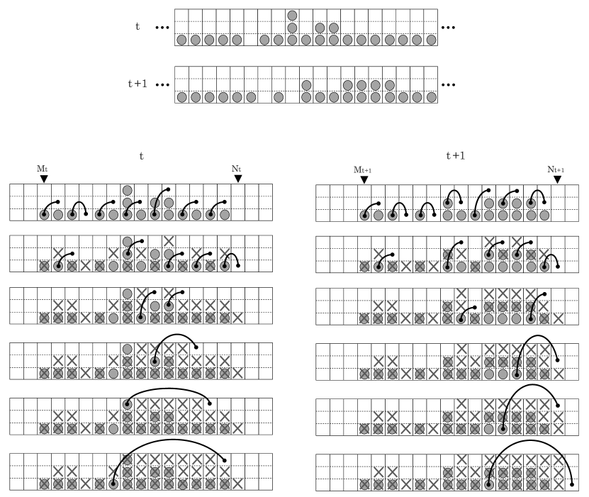
Figure 5: The scheme to count the conserved quantities of the BBS with larger capacities. We have to choose different sequences of boxes at time step $t$ and $t+1$. From this figure, we have $\tilde{q}_{1}(t)=7,\ \tilde{q}_{2}(t)=5,\ \tilde{q}_{3}(t)=2,\ \tilde{q}_{4}(t)=1,\ \tilde{q}_{5}(t)=1,\ \tilde{q}_{6}(t)=1$ and $\tilde{q}_{1}(t+1)=7,\ \tilde{q}_{2}(t+1)=5,\ \tilde{q}_{3}(t+1)=2,\ \tilde{q}_{4}(t+1)=1,\ \tilde{q}_{5}(t+1)=1,\ \tilde{q}_{6}(t+1)=1$. Since $M=1$, $N_{t}-M_{t}=14$ and $N_{t+1}-M_{t+1}=14$, we obtain $q_{1}=7-\frac{14}{2}=0,\ q_{2}=5-\frac{14}{2}=-2,\ q_{3}=2,\ q_{4}=q_{5}=q_{6}=1$ in both time steps.

The statement of the proposition is the direct consequence of the fact that $\displaystyle\sum_{i=1}^{k}\tilde{q_{i}}$ is equal to the number of balls moved by the carrier with capacity $k$ at one time step which is the value of $k$th energy function[11, 12]. Here we map the system to the BBS with box capacity $2M+1$ in which the number of balls is finite, that is, the $n$th box is vacant for $n\leq M_{t}-1$ and $N_{t}\leq n$. Of course we can make another choice. We could impose the condition $N_{t}-M_{t}\equiv 1$ (mod $2$) or the condition that a vacancy in the $N_{0}$th box is connected by an arcline in the first step. This redundancy is caused by the fact that there are essentially four types of finite systems which are equivalent to this system. Once we determine the type however, the sequence $(q_{1},q_{2},\ldots)$ does not depend on $N_{t}$ and $M_{t}$ as long as they are sufficiently large and, when there is no negative soliton $q_{2M+j}=\hat{q}_{j}$ $(j=1,2,\ldots)$, where $\hat{q}_{j}$ is the $j$th conserved quantity defined in the original BBS.

3 Soliton solutions interacting with a background state

For the original BBS where every box capacity is one and only a finite number of balls exist, all the solutions are proved to be constructed by ultradiscretization from the soliton solutions of the discrete KdV equation (6)[16]. Although the ultradiscrete KdV equation (1) over arbitrary integers is shown to be equivalent to the BBS with larger box capacity, the solutions to them can not be the ultradiscrete limit of soliton solutions to (6), because the boundary condition of the BBS changes such that the number of balls becomes $M$ for $|n|\to\infty$. Nevertheless we shall show that solutions can be constructed from the soliton solutions to (6) through ultradiscretization with an appropriate scaling limit. Here we treate only the case $M=1$. Our method for constructing the solutions is equally applicable to the case $M\geq 2$, although the analysis of that case is more elaborate.

The coupled equations for the BBS are explicitly written as

$$U_{n}^{t+1} =\min\left[3-U_{n}^{t},V_{n}^{t}\right],$$ (11)

$$V_{n+1}^{t} =U_{n}^{t}+V_{n}^{t}-U_{n}^{t+1},$$ (12)

with the boundary condition

$$\lim_{|n|\to\infty}U_{n}^{t}=\lim_{|n|\to\infty}V_{n}^{t}=1.$$ (13)

From (2) and (3), if we put $\displaystyle\delta=e^{-L/\epsilon}$ ($L\in{\mathbb{Z}}_{+}$) and assume that

$$\rho_{n}^{t}:=\lim_{\epsilon\to+0}\epsilon\log\sigma_{n}^{t}$$

exists, we find

$$\rho_{n+1}^{t+1}+\rho_{n}^{t-1}=\max\left[\rho_{n+1}^{t-1}+\rho_{n}^{t+1}-L,\rho_{n}^{t}+\rho_{n+1}^{t}\right].$$ (14)

From (3), if we put

$$U_{n}^{t} =\rho_{n}^{t}-\rho_{n}^{t-1}-\rho_{n+1}^{t}+\rho_{n+1}^{t-1},$$ (15)

$$V_{n}^{t} =\rho_{n+1}^{t}-2\rho_{n}^{t}+\rho_{n-1}^{t},$$ (16)

they satisfy (11) and (12) for $L=3$. Hence we will construct solutions $\rho_{n}^{t}$ of (14) which satisfy the boundary conditions (13).

First let us consider a state where only negative solitons exist. The corresponding solution is called a background solution [7]. It is a stationary solution of the form $\displaystyle U_{n}^{t}=F(n-t)$ where $\displaystyle\;\{F(k)\}_{k=-\infty}^{\infty}$ is a $01$ sequence with only finite number of $0$s. Let the number of $0$s be $s+1$ ($s\in{\mathbb{Z}}_{\geq 0}$), and let $b_{0}=\delta_{0}=0$, $b_{i}\in{\mathbb{Z}}_{\geq 0}$ ($i=1,2,\ldots,s$) and $\delta_{i}\in\{0,1\}$ $(i=1,2,\ldots,s)$. We define a $01$ sequence $\displaystyle\{\tilde{F}(k)\}_{k=-\infty}^{\infty}$ as

$$\tilde{F}(k)=\left\{\begin{array}[]{cl}0&\;\;k=-\sum_{i=0}^{j}(2b_{i}+\delta_{i}+i)\;(j=0,1,2,\ldots,s),\\ 1&\;\;\qquad\mbox{otherwise}.\end{array}\right.$$ (17)

Apparently any background solution $F(k)$ can be expressed as $F(k)=\tilde{F}(k-a)$ for some integers $a,\ s,\ \{b_{i}\}\$ and $\{\delta_{i}\}$.

The $N$ soliton solution to (2) is given as

$$\sigma_{n}^{t}=1+\sum_{{J\subseteq[N]}\atop{J\neq\phi}}\left(\prod_{i\in J}(-\gamma_{i})\left(\frac{1-p_{i}}{p_{i}}\right)^{t}\left(\frac{p_{i}+\delta}{1+\delta-p_{i}}\right)^{n}\right)\frac{\prod_{i>j,i,j\in J}(p_{i}-p_{j})^{2}}{\prod_{i,j\in J}(1-p_{i}-p_{j})},$$ (18)

where $p_{i}\in{\mathbb{C}}$ and $\gamma_{i}\in{\mathbb{C}}$ $(i=1,2,\ldots,n)$ are arbitrary but $p_{i}\neq p_{j}$ for $i\neq j$[4, 5]. We often denote $[k]:=\{1,2,3,\ldots,k\}$ for a positive integer $k$. To take the ultradiscrete limit, let $\displaystyle\delta=e^{-L/\epsilon}$, $\displaystyle p_{i}=N_{i}e^{-P_{i}/\epsilon}$, $\displaystyle-\gamma_{i}=M_{i}e^{-C_{i}/\epsilon}$ $(i=1,2,\ldots,N)$ where $C_{i}\in\mathbb{R},\ L,P_{i},N_{i},M_{i}>0$ and $N_{i}\neq N_{j},\ M_{i}\neq M_{j}$ for $i\neq j$. Then taking the limit $\displaystyle\lim_{\epsilon\to+0}\epsilon\log\sigma_{n}^{t}=:\rho_{n}^{t}$, we have

$$\rho_{n}^{t}=\max\left\{0,\max_{{J\subseteq[N]}\atop{J\neq\phi}}\left[\sum_{i\in J}(C_{i}+tP_{i}-n\min[P_{i},L])-\sum_{{i,j\in J}\atop{i\neq j}}\min[P_{i},P_{j}]\right]\right\}.$$ (19)

For $L=1$, we find that $U_{n}^{t}$ and $V_{n}^{t}$ satisfy (7) and (8), and hence (1). In particular, if $P_{i}\in{\mathbb{Z}}_{+},\ C_{i}\in{\mathbb{Z}}$, (19) gives an $N$ soliton solution of the original BBS.

We are, however, concerned with Eqs. (11) and (12) with the boundary condition (13). Hereafter we put $L=3$ and prepare several symbols and notations:

$$l: =\sum_{i=1}^{s}\delta_{i},\quad\delta_{s+1}\equiv s-l+1\;\;(\mbox{mod}\ 2),\quad l^{\prime}:=l+\delta_{s+1},$$

$$K: =l+\sum_{i=1}^{s}b_{i},\quad B_{i}:=\sum_{j=0}^{i}b_{j},\quad\Delta_{i}:=\sum_{j=0}^{i}\delta_{i},$$

We also assume that $\delta_{i}=1$ for $i=m_{1},m_{2},\ldots,m_{l}$ ($1\leq m_{1}<m_{2}<\cdots<m_{l}\leq s$), and $m_{l+1}:=s+1$. Let us consider an $n_{\infty}$ soliton solution $(n_{\infty}\gg 1)$ of the form (19). We assume that $P_{i}=2$ ($1\leq i\leq n_{\infty}-l^{\prime}$) and $P_{i}^{\prime}:=P_{i+n_{\infty}-l^{\prime}}=1$ $(1\leq i\leq l^{\prime})$. The phases are chosen as

$$C_{i} =\left\{\begin{array}[]{cl}\displaystyle 1&(1\leq i\leq n_{0}),\\ \displaystyle-2j+1&(n_{0}+B_{j-1}+1\leq i\leq n_{0}+B_{j}\;\;(j=1,2,...,s)),\\ \displaystyle-2s-1&(n_{0}+B_{s}+1\leq i),\end{array}\right.$$

$$C_{i}^{\prime} \equiv C_{i+n_{\infty}-l^{\prime}}:=-(m_{i}-i)\;\;(i=1,2,...,l^{\prime}).$$

Then we find

$$\rho_{n}^{t} =\max_{{0\leq k_{1}\leq n_{\infty}-l^{\prime}}\atop{0\leq k_{2}\leq l^{\prime}}}\left[\sum_{i=1}^{k_{1}}(C_{i}-2(n-t))+\sum_{i=1}^{k_{2}}(C_{i}^{\prime}-(n-t))\right.$$

$$\qquad\qquad-2k_{1}(k_{1}-1)-k_{2}(k_{2}-1)-2k_{1}k_{2}\Biggr{]}$$

$$=\max_{{-n_{0}\leq k_{1}\leq n_{\infty}-l^{\prime}-n_{0}}\atop{0\leq k_{2}\leq l^{\prime}}}\left[-(2k_{1}+k_{2})(n-t+2n_{0})+{\sum_{i=1}^{k_{1}}}^{\prime}\bar{C}_{i}\right.$$

$$\qquad\left.+\sum_{i=1}^{k_{2}}C_{i}^{\prime}-2k_{1}(k_{1}-1)-k_{2}(k_{2}-1)-2k_{1}k_{2}\right]$$

$$\qquad\qquad\qquad\qquad\qquad-2n_{0}(n-t+2n_{0})+2n_{0}^{2}+3n_{0},$$

where

$$\bar{C}_{i} :=C_{n_{0}+i},$$

$${\sum_{i=1}^{k}}^{\prime}\bar{C}_{i} :=\left\{\begin{array}[]{cl}\displaystyle\sum_{i=1}^{k}\bar{C}_{i}&\quad(k\geq 1),\\ k&\quad(k\leq 0).\end{array}\right.$$

It is obvious that if $\rho_{n}^{t}$ is a solution to (14), $\displaystyle\rho_{n+b}^{t+c}+at+f(n)$ is also a solution for an arbitrary function $f(n)$ and arbitrary values $a,\ b$ and $c$. Hence we find that $\rho_{n}^{t}=\rho_{n_{0},n_{\infty}}(n-t)$ is a solution to (14), where

$$\rho_{n_{0},n_{\infty}}(x) =\max_{{-n_{0}\leq k_{1}\leq n_{\infty}-l^{\prime}-n_{0}}\atop{0\leq k_{2}\leq l^{\prime}}}$$

$$\quad\left[-(2k_{1}+k_{2})x+{\sum_{i=1}^{k_{1}}}^{\prime}\bar{C}_{i}+\sum_{i=1}^{k_{2}}C_{i}^{\prime}\right.$$

$$\qquad\qquad-2k_{1}(k_{1}-1)-k_{2}(k_{2}-1)-2k_{1}k_{2}\Biggr{]}.$$

Since $n_{0},\ n_{\infty}$ are large but arbitrary positive integers, the limit

$$\rho_{F}(x) :=\lim_{n_{0}\to\infty}\lim_{n_{\infty}\to\infty}\rho_{n_{0},n_{\infty}}(x)$$

$$=\max_{{k_{1}\in{\mathbb{Z}}}\atop{0\leq k_{2}\leq l^{\prime}}}\left[-(2k_{1}+k_{2})x+{\sum_{i=1}^{k_{1}}}^{\prime}\bar{C}_{i}\right.$$

$$\quad\left.\qquad+\sum_{i=1}^{k_{2}}C_{i}^{\prime}-2k_{1}(k_{1}-1)-k_{2}(k_{2}-1)-2k_{1}k_{2}\right]$$ (20)

is also a solution to (14).

When we rewrite in (14) as

$$\max_{r\in{\mathbb{Z}}}\left[-rx+\max_{{0\leq k_{2}\leq l^{\prime}}\atop{2k_{1}+k_{2}=r}}\left[{\sum_{i=1}^{k_{1}}}^{\prime}\bar{C}_{i}+\cdots\right]\right]$$

and using the relations such as

$$a_{0}+a_{2}\geq 2a_{1}\ \longrightarrow\ \max[-2x+a_{2},-x+a_{1},a_{0}]=\max[-2x+a_{2},a_{0}]$$

Eq. (20) can be simplified as shown in the Proposition 2 below. First let us define some symbols and notations.

$$C_{T} :=\sum_{j=1}^{s}(2j-1)b_{j}+\sum_{j=1}^{l}(m_{j}-j),\quad Q_{0}:=C_{T}+K(K-1)+(K-l)(K-l-1)$$

$$S_{1} :=\{m_{1},m_{2},\ldots,m_{l}\},\quad S_{0}:=[l]\setminus S_{1},\quad I:=[2K-l]\setminus\bar{I}$$

$$\bar{I} :=\left\{m\in[2K-l]\Big{|}m=2B_{i-1}+\Delta_{i-1}+2k_{i}+1,\ k_{i}=0,1,\ldots,b_{i-1}-1,\ i\in S_{0}\right\}$$

The quantity $\Theta_{r}$ is defined for $r\in I$ as

• If $i\in S_{0}$ and $\displaystyle 2B_{i-1}+\Delta_{i-1}+2\leq r\leq 2B_{i}+\Delta_{i}$, then putting $r=2B_{i-1}+\Delta_{i-1}+2k$ $\ (k\in\mathbb{Z})$,

  $$\Theta_{r} :=\sum_{j=1}^{i-1}\left[(2j-1)b_{j}+(j-\sum_{\mu=1}^{j}\delta_{\mu})\delta_{j}\right]+(2i-1)k$$

  $$\quad+(B_{i-1}+k+\Delta_{i-1})(B_{i-1}+k+\Delta_{i-1}-1)+(B_{i-1}+k)(B_{i-1}+k-1).$$ (21)

• If $i\in S_{1}$, $\displaystyle 2B_{i-1}+\Delta_{i-1}+1\leq r\leq 2B_{i}+\Delta_{i}$ and $r=2B_{i-1}+\Delta_{i-1}+2k$ $\ (k\in\mathbb{Z})$, then $\Theta_{r}$ is given by (21).

• If $i\in S_{1}$, $\displaystyle 2B_{i-1}+\Delta_{i-1}+1\leq r\leq 2B_{i}+\Delta_{i}$ and $r=2B_{i-1}+\Delta_{i-1}+2k+1$ $\ (k\in\mathbb{Z})$, then

  $$\Theta_{r} :=\sum_{j=1}^{i-1}(2j-1)b_{j}+\sum_{j=1}^{i}(j-\sum_{\mu=1}^{j}\delta_{\mu})\delta_{j}+(2i-1)k$$

  $$\quad+(B_{i-1}+k+\Delta_{i})(B_{i-1}+k+\Delta_{i}-1)+(B_{i-1}+k)(B_{i-1}+k-1).$$ (22)

Proposition 2

$$\rho_{F}(x):=\max\left[\rho_{F}^{(-)}(x),\rho_{F}^{(0)}(x),\rho_{F}^{(+)}(x)\right],$$ (23)

where

$$\rho_{F}^{(-)}(x) :=\max_{{k\geq 0}\atop{k\in\mathbb{Z}}}\left[(2x-1)k-2k(k+1)\right],$$ (24)

$$\rho_{F}^{(+)}(x) :=\left\{\begin{array}[]{l}\displaystyle\max_{{q\geq 1}\atop{q\in\mathbb{Z}}}\left[-(2K-l+2q)x-q(2q+4K-2l+2s-1)-Q_{0}\right]\quad(\delta_{s+1}=0),\\ \displaystyle\max_{{q\geq 1}\atop{q\in\mathbb{Z}}}\left[-(2K-l+q)x-(q-1)\left(\frac{q}{2}+2K-l+s\right)-s-Q_{0}\right]\quad(\delta_{s+1}=1),\end{array}\right.$$ (27)

$$\rho_{F}^{(0)}(x) :=\max_{{1\leq r\leq 2K-l}\atop{r\in{\mathbb{Z}}}}\left[\rho^{(r)}(x)\right],$$ (28)

and the function $\rho^{(r)}(x)$ is given as

$$\rho^{(r)}(x):=\left\{\begin{array}[]{cl}-rx-\Theta_{r}&\quad r\in I,\\ 0&\quad r\notin I.\end{array}\right.$$

From (15), if we define

$$U_{F}(x):=\rho_{F}(x+2)-2\rho_{F}(x+1)+\rho_{F}(x),$$ (29)

$\displaystyle U_{n}^{t}=U_{F}(n-t)$ gives a solution to (11) and (12). By using the fact that $\rho_{F}(x)$ is a continuous and convex piecewise linear function, and by calculating the intersection points of each linear functions appeared as linear pieces in the function $\rho_{F}(x)$, we obtain the explicit form of $U_{F}(x)$. Let us define $t_{i}(x)$ $(i=1,2,...)$ as

$$t_{1}(x) :=\left\{\begin{array}[]{cl}x+2&\;(-2\leq x\leq-1),\\ -x&\;(-1\leq x\leq 0),\\ 0&\;\mbox{otherwise},\end{array}\right.$$

$$t_{2}(x) :=\left\{\begin{array}[]{cl}2x+5&\;(-5/2\leq x\leq-3/2),\\ -2x-1&\;(-3/2\leq x\leq-1/2),\\ 0&\;\mbox{otherwise},\end{array}\right.$$

$$t_{2k+1}(x) :=\sum_{i=0}^{2k}t_{1}(x+i),$$

$$t_{2k}(x) :=\sum_{i=0}^{k-1}t_{2}(x+2i).$$

By straightforward but a little tedious calculation, we find

$$U_{F}(x)=U_{F}^{(-)}(x)+U_{F}^{(0)}(x)+U_{F}^{(+)}(x),$$ (30)

where

$$U_{F}^{(-)}(x) :=\sum_{k=1}^{\infty}t_{2}(x-2k-1),$$ (31)

$$U_{F}^{(+)}(x) :=\left\{\begin{array}[]{cl}\displaystyle\sum_{k=0}^{\infty}t_{2}(x+K+s+2k)&\;\mbox{($\delta_{s+1}=0$)},\\ \displaystyle\sum_{k=0}^{\infty}t_{1}(x+K+s+k)&\;\mbox{($\delta_{s+1}=1$)},\end{array}\right.$$ (34)

$$U_{F}^{(0)}(x) :=\sum_{i=1}^{s}t_{2b_{i}+\delta_{i}}(x+2B_{i-1}+\Delta_{i-1}+i-1).$$ (35)

An example of the function $U_{F}(x)$ is shown in figure 6. Comparing these expressions with $\tilde{F}(k)$, we find that $\displaystyle U_{F}(k)=\tilde{F}(k)$ for $k\in{\mathbb{Z}}$. Thus we have proved the following proposition.

Proposition 3

It holds that $U_{F}(k)=\tilde{F}(k)$ for $k\in{\mathbb{Z}}$.

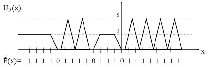
Figure 6: An example of $\tilde{F}(x)$ and $U_{F}(x)$. The parameters are $b_{1}=1,\ \delta_{1}=1,\ b_{2}=2,\ \delta_{2}=0$.

Furthermore, comparing $\tilde{F}(k)$ with the conserved quantities $\{q_{j}\}$ defined in the previous section, we have the following proposition.

Proposition 4

The number of negative solitons is equal to $-q_{1}-q_{2}$, i.e., $s+1=-q_{1}-q_{2}$, and $q_{1}-q_{2}$ is the number of solitons with amplitude $1$ which is used to construct the background solution, i.e., $q_{1}-q_{2}=l^{\prime}$.

Next we consider the solutions in which $m$ ordinary solitons exist in a background state. Since $N$ soliton solutions are given by (19) and the parameters for the background solution are already known, we have only to add new parameters $\displaystyle\{\hat{P}_{i}\}_{i=1}^{m}$ $({}^{\forall}i\ \hat{P}_{i}\geq 3)$ and $\displaystyle\{\hat{C}_{i}\}_{i=1}^{m}$. When we denote the set of indices for a background solution $\mathcal{B}$, then the solution is given by

$$\rho_{n}^{t} =\max_{J_{1}\subseteq[m],J_{2}\subseteq\mathcal{B}}\left[\sum_{i\in J_{1}}(-\min[3,\hat{P}_{i}]n+\hat{P}_{i}t+\hat{C}_{i})+\sum_{i\in J_{2}}(-P_{i}(n-t)+C_{i})\right.$$

$$\qquad-\sum_{i\neq j,i,j\in J_{1}}\min[\hat{P}_{i},\hat{P}_{j}]-\sum_{i\neq j,i,j\in J_{2}}\min[P_{i},P_{j}]-2\sum_{i\in J_{1},j\in J_{2}}\min[\hat{P}_{i},P_{j}]\Biggr{]}$$

$$=\max_{J_{1}\subseteq[m],J_{2}\subseteq\mathcal{B}}\left[\sum_{i\in J_{1}}(-3n+\hat{P}_{i}t+\hat{C}_{i})+\sum_{i\in J_{2}}(-P_{i}(n-t)+C_{i})\right.$$

$$\qquad-\sum_{i\neq j,i,j\in J_{1}}\min[\hat{P}_{i},\hat{P}_{j}]-\sum_{i\neq j,i,j\in J_{2}}\min[P_{i},P_{j}]-2\sum_{j\in J_{2}}|J_{1}|P_{j}\Biggr{]}$$

$$=\max_{J_{1}\subseteq[m]}\left[\sum_{i\in J_{1}}(-3n+\hat{P}_{i}t+\hat{C}_{i})-\sum_{i\neq j,i,j\in J_{1}}\min[\hat{P}_{i},\hat{P}_{j}]\right.$$

$$\qquad+\max_{J_{2}\subseteq\mathcal{B}}\left.\left[\sum_{i\in J_{2}}(-P_{i}(n-t+2|J_{1}|)+C_{i})-\sum_{i\neq j,i,j\in J_{2}}\min[P_{i},P_{j}]\right]\right].$$

Here we used the abbreviation

$$\max_{J\subseteq\mathcal{A}}\left[\cdots\right]\equiv\max\left\{0,\max_{J\subseteq\mathcal{A},J\neq\phi}\left[\cdots\right]\right\}.$$

Therefore we obtain the following theorem.

Theorem 1

The solution to (14) representing the interaction of $m$ soliton solutions with the background given by (23), has the expression:

$$\rho_{n}^{t}=\max_{J\subseteq[m]}\left[\sum_{i\in J}(-3n+\hat{P}_{i}t+\hat{C}_{i})-\sum_{{i\neq j}\atop{i,j\in J}}\min[\hat{P}_{i},\hat{P}_{j}]+\rho_{F}(n-t+2|J|)\right].$$ (36)

The multi-soliton solutions with a background is also given by Y. Nakata in an algebraic form (nested maximization) with the ultaradiscrete vertex operators[18]. So far we do not find the exact correspondence between our solution (36) and his formula.

From (36), we find that the phase shift of negative solitons after collision of an ordinary soliton is $-2$. An example of a time evolution pattern is shown in figure 7. Since the solution (36) shows that the ordinary solitons move freely for $t\gg 1$ as those in the BBS with box capacity one, comparing with the construction of conserved quantities, we find the following proposition[17].

Proposition 5

For a solution to (1) determined by (36), let $Y$ be the Young diagram corresponding to the partition $(q_{3},q_{4},q_{5},\cdots)$ constituted by the conserved quantities, that is, the length of its $i$th column of $Y$ is $q_{i+2}$. Then, the length of $j$th row in $Y$ is equal to $\hat{P}_{j}-2$.

Figure 7: A solution $U_{n}^{t}$ given by (36). Here $U_{n}^{t}=\rho_{n}^{t}-\rho_{n}^{t-1}-\rho_{n+1}^{t}+\rho_{n+1}^{t-1}$. The symbol ‘.’ denotes ‘1’. The parameters are $\hat{P}_{1}=4,\ \hat{C}_{1}=-7,\ \hat{P}_{2}=7,\ \hat{C}_{2}=-5,\ b_{1}=2,\ \delta_{1}=0,\ b_{2}=1,\ \delta_{2}=1$. When we make gage transformation as $U_{n}^{t}-1\to U_{n}^{t}$, this time evolution pattern coincides with that of figure 4.

4 Concluding remarks

We constructed the conserved quantities of the ultradiscrete KdV equation (1) with negative solitons by using the transformation to the BBS with larger box capacities. The solutions to (1) in which negative solitons and ordinary solitons coexist are also obtained as the solutions to this extended BBS. In the BBS with box capacity one, every state is obtained by ultradiscretization of a soliton solution of the discrete KdV equation, and using this fact, initial value problem is solved with elementary combinatorial methods. We conjecture that this fact also holds for the extended BBS and can be used to solve the initial value problems. Investigating this conjecture is a problem we wish to address in the future.

References

[1]
D. Takahashi and J. Satsuma 1990
“A soliton cellular automaton”,
J. Phys. Soc. Jpn.59, 3514–3519
[2]
D. Takahashi 1993
“On some soliton systems defined by using boxes and balls”,
Proc. Int. Symp. on Nonlinear Theory and its Applications (NOLTA’93), 555–558
[3]
M. Torii, D. Takahashi and J. Satsuma 1990
“Combinatorial representation of invariants of a soliton cellular automaton”,
PhysicaD92, 209–220
[4]
T. Tokihiro, D. Takahashi, J. Matsukidaira and J. Satsuma 1996
“From soliton equations to integrable cellular automata through
a limiting procedure”,
Phys. Rev. Lett.76, 3247–3250
[5]
R. Hirota, S. Tsujimoto and T. Imai 1992
“Difference Scheme of Soliton Equations”,
Future directions of nonlinear dynamics in physical and biological systems
NATO Adv. Sci. Inst. Ser. B: Phys.312, Plenum, 7–15
[6]
R. Hirota 2009
“New Solutions to the Ultradiscrete Soliton Equations”,
Stud. Appl. Math.122, 361–376
[7]
R. Willox, Y. Nakata, J. Satsuma, A. Ramani and B. Grammaticos 2010
“Solving the ultradiscrete KdV equation”,
J. Phys. A: Math. Theor.43, 482003, 7pp
[8]
D. Takahashi and J. Matsukidaira 1997
“Box and ball system with a carrier and ultradiscrete modified KdV equation”,
J. Phys. A: Math. Gen.30, L733–739
[9]
M. Murata, S. Isojima, A. Nobe and J. Satsuma 2006
“Exact solutions for discrete and ultradiscrete modified KdV equations and their relation to box-ball systems”,
J. Phys. A: Math. Gen.39, L27–34
[10]
A. Nakayashiki and Y. Yamada 1997
“Kostka polynomials and energy functions in solvable lattice models”,
Selecta Mathematica, New Ser.3, 547–599
[11]
K. Fukuda, M. Okado and Y. Yamada 2000
“Energy functions in box ball systems”,
Int. J. Mod. Phys. A15, 1379–1392
[12]
G. Hatayama, K. Hikami, R. Inoue, A. Kuniba, T. Takagi and T. Tokihiro 2001
“The automata related to crystals of symmetric tensors”,
J. Math. Phys.42, 274–308
[13]
This transformation was independently found out by C. Gilson, A. Nagai and J. Nimmo.
(private communication).
[14]
J. Mada, M. Idzumi and T. Tokihiro 2005
“Path description of conserved quantities of generalized periodic box-ball systems”,
J. Math. Phys.46, 022701, 19pp
[15]
K. Fukuda 2004
“Box-ball systems and Robinson-Schensted-Knuth correspondence”,
J. Algebraic Combin.19, 67–89
[16]
J. Mada, M. Idzumi and T. Tokihiro 2008
“The box–ball system and the -soliton solution of the ultradiscrete KdV equation”,
J. Phys. A: Math. Theor.41, 175207, 23pp
[17]
D. Yoshihara, F. Yura and T. Tokihiro 2003
“Fundamental Cycle of a Periodic Box-Ball System”,
J. Phys. A: Math. Gen.36, 99–121
[18]
Y. Nakata 2010
“Vertex operators and background solutions for ultradiscrete soliton equations”,
Doctor Thesis, University of Tokyo