Near Infrared Photometric properties of 130,000 Quasars:
An SDSS-UKIDSS matched catalog

Abstract

We present a catalog of over 130,000 quasars candidates with NIR photometric properties, with an areal coverage of approximately 1,200 deg². This is achieved by matching the Sloan Digital Sky Survey (SDSS) in the optical ugriz bands, to the UKIRT Infrared Digital Sky Survey (UKIDSS) Large Area Survey (LAS) in the near-infrared YJHK bands. We match the $\approx 1$ million SDSS DR6 Photometric Quasar catalog to Data Release 3 of the UKIDSS LAS (ULAS), and produce a catalog with 130,827 objects with detections in one or more NIR bands, of which 74,351 objects have optical and K-band detections and 42,133 objects have the full 9-band photometry. The majority ($\sim 85\%$) of the SDSS objects were not matched simply because there were not covered by the ULAS. The positional standard deviation of the SDSS Quasar to ULAS matches is $\delta_{\rm R.A.}=0.1370^{\prime\prime}$ and $\delta_{\rm Decl.}=0.1314^{\prime\prime}$. We find an absolute systematic astrometric offset between the SDSS Quasar catalog and the UKIDSS LAS, of $|{\rm R.A._{offset}}|=0.025^{\prime\prime}$, and $|{\rm Decl._{offset}}|=0.040^{\prime\prime}$; we suggest the nature of this offset to be due to the matching of catalog, rather than image, level data. Our matched catalog has a surface density of $\approx 53$ deg^-2 for $K\leq 18.27$ objects; tests using our matched catalog, along with data from the UKIDSS DXS, implies that our limiting magnitude is $i\approx 20.6$. Color-redshift diagrams, for the optical and NIR, show the close agreement between our matched catalog and recent quasar color models at redshift $z\lesssim 2.0$, while at higher redshifts, the models generally appear to be bluer than the mean observed quasar colors. The $gJK$ and $giK$ color-spaces are used to examine methods of differentiating between stars and (mid-redshift) quasars, key to currently ongoing quasar surveys. Finally, we report on the NIR photometric properties of high, $z>4.6$, and very high, $z>5.7$, redshift previously discovered quasars.

1. Introduction

With the completion of the Sloan Digital Sky Survey (SDSS; York et al., 2000), the era of high quality, homogeneous CCD imaging over large fractions of the sky has arrived. The final data release from the SDSS, (DR7; Abazajian et al., 2009) contains over 11,000 deg² of imaging data, with 357 million unique objects being identified in a $\sim 60$ Terabyte database.

Table 1Descriptions of previous catalogs of quasars. ^aO/I, Optical or Infrared; P/S, Photometric or spectroscopic survey. ^bSDSS Faint Quasar Survey. ^cThe FIRST-2MASS Red Quasar Survey. ^dThe SDSS DR7 Quasar catalog provides NIR photometry from 2MASS for 53,584 objects, 29,551 or which are detected in the K-band. ^eThe 2MASS Second Incremental Data Release.

Survey	Area (deg2)	NQ	Magnitude Range	O/I & P/Sa	Reference
COMBO-17	0.8	192	$R<24$	O/P	Wolf et al. (2003)
SFQSb	4	414	$g<22.5$	O/S	Jiang et al. (2006)
SDSS-ULAS DR1	189	2 873	$K<18.2$	I/S	Chiu et al. (2007)
2SLAQ QSO	190	8 764	$18.00<g<21.85$	O/S	Croom et al. (2009b)
2QZ	700	23 338	$18.25<b_{\rm J}<20.85$	O/S	Croom et al. (2004)
SDSS-ULAS DR3	1 200	74 351	$K<18.4$	I/P/S	this work
FIRST-2MASS RQSc	2 716	57	$K\leq 14.3,(R-K)>4,(J-K)>1.7$	I/S	Glikman et al. (2007)
SDSS DR6pQ	8 342	1 015 082	$i<21.3$	O/P	Richards et al. (2009a)
SDSS DR7Qd	9 380	29 551	$K\lesssim 17.0$	I/S	Schneider et al. 2010
SDSS DR7Q	9 380	105 807	$i<20.2$	O/S	Schneider et al. 2010
2MASS 2IDRe	$\sim 30$ 000	2 277	$K\leq 15$	I/S	Barkhouse & Hall (2001)

The identification of quasars was a major focus of the SDSS project; utilizing the broad 5-filter photometry (Richards et al., 2002) led to efficient selection (Vanden Berk et al., 2005; Richards et al., 2006) of low, $z<2.2$, and high, $z\gtrsim 3.5$, redshift quasars, identified via their spectroscopic signatures (Schneider et al., 2010, and references therein). However, quasars can also be efficiently identified by their SDSS imaging properties alone (Richards et al., 2001), due to their point-source appearance, but non-stellar location in color-color space. With the most recent catalog of Richards et al. (2009a, hereafter R09), based on imaging from the SDSS, the number of photometrically identified quasars now stands at over 1 million. Both the SDSS spectroscopic and photometric quasar catalogs have been used to investigate global quasar properties such as the luminosity function (QLF; Fan et al., 2001; Richards et al., 2006; Croom et al., 2009a) and clustering (Myers et al., 2006; Myers et al., 2007; Shen et al., 2007, 2009; Ross et al., 2009).

The emergence of large surveys has not been confined to the optical regime. In the near-infrared (NIR; $\lambda\approx 1-5\mu$m) quasar catalogs (e.g. Barkhouse & Hall, 2001; Cutri et al., 2002; Francis et al., 2004; Ofek et al., 2007; Kouzuma & Yamaoka, 2010a, b) have been available since the completion of the 2 Micron All Sky Survey (2MASS; Skrutskie et al., 2006). Table LABEL:tab:previous_surveys summarizes how previous quasar surveys, both in the optical and NIR, compare by area, number of objects and magnitude range.

Quasar observations in the NIR are particularly important for individual objects that are seen only in the reddest, or indeed potentially none, of the optical filters (e.g. Fan et al., 2006; Venemans et al., 2007; Willott et al., 2009). Observations of the general quasar population in the K-band are key since this links the rest-frame ultraviolet (UV)/optical to the mid-infrared (MIR; $\lambda\approx 5-30\mu$m); the former being where there is the peak in the radiative output for Type I, non-obscured quasars, (e.g. Shakura & Sunyaev, 1973; Sanders et al., 1989; Kishimoto et al., 2008; Richards et al., 2009b), and the latter where reprocessed light heats intrinsic dust to $\sim 30-300$ K (e.g. Pier & Krolik, 1993; Efstathiou & Rowan-Robinson, 1995; Lacy et al., 2004). Observations in the observed K-band also measures the rest-frame i and g-bands at redshifts $z\sim 1.9$ and $z\sim 3.7$, respectively.

However, it is only the bright, $g\lesssim 16$ magnitude quasars that are detected by the relatively shallow limits of the 2MASS survey, and the majority of known quasars are fainter than this in the NIR bands. The UKIRT Infrared Deep Sky Survey (UKIDSS; Lawrence et al., 2007), a seven-year sky survey which began in 2005 May, has five different survey components. The UKIDSS “Large Area Survey” (ULAS) aims to reach $\sim 4$ magnitudes deeper than 2MASS over an area of up to 4,000 deg², directly overlapping the optical imaging footprint of the SDSS.

The primary goal of this paper is to create a catalog of over 130,000 quasars with optical, ugriz (Fukugita et al., 1996), and NIR, YJHK photometry, with an areal coverage of 1 200 deg². By matching the catalogs of R09 in the optical regime to that of the ULAS in the NIR we produce, by a factor of at least two, the largest catalog of quasars detected in the K-band. The major motivation for the catalog will be its utilization in an future study where we measure the $K$-band quasar luminosity function (Peth, Ross et al. in prep.). By concentrating on the $\approx 200$ deg² area from the SDSS known as “Stripe 82”, our K-band quasar luminosity function will show the evolution from redshift of zero to two.

The analysis by Trammell et al. (2007) is an example of the synergy produced by the matching and production of a multi-wavelength catalog. These authors match $\sim$6000 SDSS quasars to UV data provided by the Galaxy Evolution Explorer (GALEX; Martin et al., 2005) satellite and find that over 80$\%$ of the optically detected quasars have near-UV detections. The quasars are well separated from stars in UV-optical color-color space. The large sample size allows for the construction of SEDs in bins of redshift and luminosity, which shows the median SED becoming bluer at UV wavelengths for quasars with lower continuum luminosity. Ball et al. (2007) also perform catalog matching using SDSS quasar data and GALEX UV photometry, with the goal of understanding quasar photometric redshift properties.

The studies by Warren et al. (2000), Croom et al. (2001), Sharp et al. (2002) and more recently, Maddox et al. (2008) and Smail et al. (2008), are another motivation why a sample of quasars with NIR photometric properties is desired. These authors show that using a “KX selection”, where the quasar SED shows an excess in the K-band compared to a stellar SED, can successfully identify quasar candidate objects that would be normally excluded from the SDSS (optical) quasar selection algorithm - even for dust reddened quasars. This is an important result since selecting complete quasar samples via the KX method opens up the possibility of investigating the “Quasar Epoch” over the redshift range of $2.2<z<3.5$, where current, usually optically selected, quasar samples are particularly poorly represented. A similar project to Maddox et al. (2008) was Nakos et al. (2009), who also select quasar candidates using the KX-technique, where these authors identify quasars on the basis of their optical ($R$ and $z^{{}^{\prime}}$) to NIR ($K_{\rm s}$) photometry and point-like morphology. Jurek et al. (2008) also test the KX method and find that it is more effective than the traditional “UV Excess” (UVX) selection method at finding red, ($b_{\rm J}-K)\geq 3.5$, quasars.

There are two comparable studies and samples to our own work. Chiu et al. (2007) and Souchay et al. (2009), the latter recently producing the “Large Quasar Astrometric Catalog” (LQAC). Our work differs from these studies, in two key ways; (i) we have over an order of magnitude more objects in our sample compared to Chiu et al. (2007); (ii) our catalog uses UKIDSS data, as opposed to 2MASS data (Souchay et al., 2009), where the former is much better matched to the SDSS imaging depth.

This paper is organized as follows. In Section 2 we present our sample, giving a brief overview of the SDSS and UKIDSS. Section 3 lays out our catalog. In Section 4 we present $N(z)$, color-redshift and color-color relations from our matched catalog. In Section 5 we present analysis of high-redshift quasars and calculations of the i and K-band number counts. The Appendix gives further details on magnitude conversions and cross-checks of our study.

We assume the currently preferred flat, “Lambda Cold Dark Matter” ($\Lambda$CDM) cosmology where $\Omega_{\rm b}$ =0.042, $\Omega_{\rm m}$ = 0.237, $\Omega_{\Lambda}$ = 0.763 (Sánchez et al., 2006; Spergel et al., 2007) and quote distances in units of $~{}h^{-1}~{}{\rm Mpc}$ to aid in ease of comparisons with previous results in the literature. Where a value of Hubble’s Constant is assumed, e.g. for absolute magnitudes, this will be quoted explicitly. All optical magnitudes are based and quoted on the AB zero-point system (Oke & Gunn, 1983), while all NIR magnitudes are based in the Vega system, with conversions from AB to Vega given in the Appendix.

2. Data and Methods

In this section, we provide overviews of the surveys and the catalogs we utilize, and how matching was performed.

2.1. The SDSS DR6 Photometric Quasar Catalog

Details regarding the SDSS can be found in the series of SDSS Data Release papers (Abazajian et al., 2009, and references therein). Full details for the SDSS DR6 Photometric Quasar Catalog (DR6pQ) are given in R09, with Richards et al. (2004) providing the “proof-of-concept” study and Weinstein et al. (2004) providing an empirical algorithm for obtaining photometric redshifts. Here we present the details specific to our work.

The photometric imaging data for the DR6pQ is based upon the SDSS Data Release 6 (Adelman-McCarthy et al., 2008). Points sources with PSF $i$-band magnitudes between 14.5 and 21.3 are extracted from the SDSS Catalog Archive Server (CAS). We continue the convention of R09, utilizing übercalibrated magnitudes (Padmanabhan et al., 2008) which are available in the SDSS database. The übercalibrated magnitudes represent the most robust photometric measurements as they are calibrated across SDSS “stripes” to a single uniform photometric system for the entire SDSS area. All magnitudes have been corrected for Galactic extinction using the Schlegel et al. (1998) dust maps.

There are 1 015 082 objects in total in the R09 catalog across 8 342 deg². The DR6 primary imaging data cover an area of 8417 deg², although as noted in R09, due to cuts the total effective area covered by this catalog is reduced by $\sim$75 deg².

2.2. The UKIRT Infrared Deep Sky Survey

Lawrence et al. (2007) gives the general overview for UKIDSS. In brief, the UKIDSS is a collection of five surveys of different coverage and depth and using WFCAM (Casali et al., 2007) on UKIRT. WFCAM has an instantaneous field of view of 0.21 deg², and the various surveys employ up to five filters, ZYJHK, covering the wavelength range 0.83-2.37$\mu$m. The photometric system and calibration are described in Hewett et al. (2006) and Hodgkin et al. (2009), respectively. The pipeline processing is described in Irwin et al. (2010, in prep.) and the WFCAM Science Archive (WSA) by Hambly et al. (2008). The processed right ascension and declination data are accurate to 0.1 arcsec. We have used data from the worldwide 4th data release, DR3, which is described in detail by Warren et al. (2010, in prep.). For this paper, we concentrate on the Large Area Survey and the Deep Extragalactic Survey.

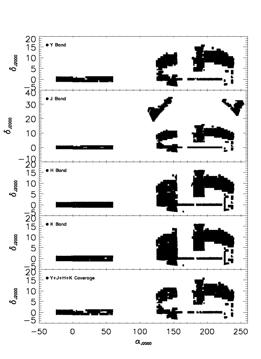
Figure 1.— Coverage over the entire UKIDSS area in each of the 4 NIR bands and finally in all 4 NIR bands simultaneously. Uses no projection, with axes in degrees for both Right Ascension and Declination. Displays $YJHK$ coverage in descending order, followed by coverage in all four bands.

2.2.1 UKIDSS LAS

The ULAS aims to map a large fraction of the Northern Sky, $\sim 4000$ deg², which, when combined with the SDSS, produces an atlas covering almost an octave in wavelength. The target depths of the survey are $Y=20.3,J=19.5,H=18.6,K=18.2$ (Vega), and the ULAS does not image in the WFCAM $Z$-band. The ULAS data for our matched catalog came courtesy of private communications with Mike Read from the WSA. Unlike the SDSS, the ULAS multiband photometry is not taken in one observation (e.g. Sec. 5.2 of Dye et al., 2006; Lawrence et al., 2007, Sec. 4.2). Therefore the four bands can, and do, have different coverage maps, with the H and K bands obtained together, and Y and J done separately. The ULAS DR3 coverage is 903 deg², 1,161 deg², 1,091 deg² and 1,111 deg² in Y, J, H and K respectively. Note that the ultimate 7-year ULAS goal is to cover 4028 deg², in each filter, and have two passes of the entire ULAS area with the J filter. The DR3 coverage of each of the four bands, and for all four bands, is shown in Figure 1. The joint coverage of all four bands is 801 deg².

2.2.2 UKIDSS DXS

The UKIDSS Deep Extragalactic Survey (DXS) plans to cover 35 deg² of sky to a 5$\sigma$ point-source sensitivity of J=22.3 and K=20.8 in four specifically selected multiwavelength survey areas. The locations and areas of these four fields, XMM-LSS, Lockman Hole, ELAIS N1 and SA22 (a.k.a VIMOS-4), are given in Table 5 of Lawrence et al. (2007). Three of these, the Lockman Hole, ELAIS N1 and SA22 fields, are covered by the R09 DR6pQ catalog. We shall therefore use the DXS data to test the faint end and limiting magnitude of the optical and NIR matched quasar catalogs.

2.3. SDSS Stripe 82

Stripe 82 is a 300 deg² area of repeat photometry on a 2.5 degree wide stripe, centered on the celestial equator in the Southern Galactic Cap and running from 300^∘ to 60^∘ in R.A. (Sec. 3.2, Abazajian et al., 2009). Co-addition of the best of this data means that optical imaging on Stripe 82 can reach roughly 2 magnitudes fainter than the main survey and as we shall see in section 5.2, this deeper imaging was used by Jiang et al. (2009) to discover new, very high, $z\sim 6$, redshift quasars. We do not require this deeper imaging for the preparation of our SDSS-ULAS matched catalog. However, due to the fact that there is almost complete coverage in the ULAS, as well as many other multi-wavelength surveys, along with the regular rectangular geometry (that will simplify the number counts and luminosity function calculations in future work), we utilize heavily the data from this area.

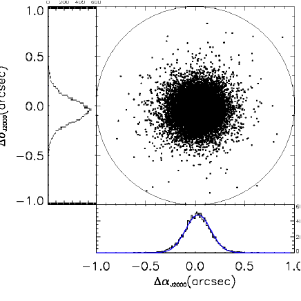
Figure 2.— The differences in Right Ascension and Declination recorded by SDSS against that recorded by the ULAS for all 17,835 matched objects in Stripe 82. A circle of radius 1^′′ is shown.

2.4. Matching Procedure

Our matching procedure is conceptually straight-forward, though is made relatively cumbersome by the shear number of objects to process. Before the million strong catalog (DR6pQ) was uploaded, tests were perform using the “CrossID” form. The positions of the 1,015,082 objects from the DR6pQ catalog were uploaded to the WFCAM Science Archive. To count as a match, the returned NIR object must be the closest object in the ULAS to the SDSS coordinates, selected from within a circle of radius 1^′′ (though we note a more stringent 0.5$"^{\prime}$ matching radius returns essentially identical results). As long as at least 1 NIR band contained a non-default, i.e. not -9.9999$\times 10^{8}$ value, the object was considered a good match. Table 2 shows the total number of objects in the R09 catalog and the number of those objects that are matched to ULAS and DXS separately, both for the full DR6pQ coverage and specifically Stripe 82.

Table 2Overall Catalog Numbers.

Catalogs	Full DR6	Stripe 82
Ri09	1,015,082	36,625
DR6pQ-ULAS Matches (in $\geq$1 NIR band)	130,827	17,835

We also perform matching tests where we offset the right ascension and declination of Stripe 82 DR6pQ catalog objects and then upload them to WSA to observe the probability of spurious matches. Table 3 shows the results of our matching tests. Once the offsets are increased to more than 1” the amount of spurious “matches” drops off precipitously.

Table 3Spurious match counts. Results of secondary matching tests where we offset the right ascension and declination of Stripe 82 DR6pQ catalog objects and then upload them to WSA to observe the probability of spurious matches.

Offset	R.A. offset “matches”	Decl. offset “matches”
1”	7253	10965
2”	56	40
5”	75	72
10”	84	93
60”	76	78

Figure 2 displays the separation in arcseconds between our matched objects in the SDSS and UKIDSS. The histograms, with a bin size of 0.01^′′ running along the sides of the plot, represent the distribution of the Right Ascension and Declination separations. We find the standard deviation of these histograms to be $\delta_{\rm R.A.}=0.1370^{\prime\prime}$ and $\delta_{\rm Decl.}=0.1314^{\prime\prime}$. These values compare very well to those determined in the UKIDSS Early Data Release paper (EDR; Dye et al., 2006) and by Chiu et al. (2007). Also similar to Chiu et al. (2007), we find an absolute offset between the SDSS and ULAS of $|{\rm R.A._{offset}}|=0.025^{\prime\prime}$, and $|{\rm Decl._{offset}}|=0.040^{\prime\prime}$. We suggest the origin of this offset to be due to the matching of catalogs, rather than image level data, and is not due to the astrometric calibration of either of the surveys, nor the size of CCD pixels (the SDSS camera pixel size is 24 $\mu$m/0^′′.396 on the sky; WFCAM pixels are 18$\mu$m/0^′′.4 on the sky). However, we also suggest this issue warrants further investigation.

Table 4The first ten objects in our NIR-matched quasar catalog. The catalog will be published in its entirety in the electronic edition of the Astrophysical Journal. The first 10 rows, of 130,827 total, are shown here.

No.	Name	SDSS ID	ULAS ID	R.A.SDSS	Decl.SDSS	$\Delta_{\rm R.A.}$	$\Delta_{\rm Decl.}$	Diff
1	000001.38-010852.2	588015507658768592	433825841152	0.0057816	-1.1478427	-0.180	0.001	0.180
2	000001.93-001427.5	588015508732510344	433822400512	0.0080576	-0.2409745	-0.130	-0.137	0.189
3	000006.42+005206.3	588015510343123177	433816469504	0.0267757	0.8684207	0.031	-0.316	0.318
4	000006.53+003055.2	588015509806252150	433817550848	0.0272281	0.5153489	0.118	0.164	0.202
5	000007.58+002943.3	588015509806252166	433817550848	0.0316036	0.4953744	-0.039	0.127	0.133
6	000008.13+001634.6	588015507658768713	433819123712	0.0338984	0.2763040	-0.077	0.108	0.132
7	000009.31-010703.1	588015507658768768	433825644544	0.0387928	-1.1175526	-0.050	0.105	0.117
8	000011.96+000225.3	588015509269381139	433820860416	0.0498422	0.0403718	-0.064	-0.078	0.101
9	000012.25-003220.5	587731185667080338	433823776768	0.0510761	-0.5390492	0.033	-0.316	0.317
10	000012.27-010405.5	588015507658768732	433825841152	0.0511651	-1.0682041	-0.062	0.193	0.203

Table 5Format of our Matched catalog. With field names and descriptions.

Column	Field	Format	Description
1	Catalog number	I5	Internal catalog object number
2	Name	A18	IAU format object name; SDSS Jhhmmss.ss$\pm$ddmmss.s
3	SDSS - ID	I18	SDSS Database ID
4	UKIDSS - ID	I12	ULAS MergedSource Database ID
5	R.A. SDSS	F12.7	R.A. J2000 (deg)
6	Decl. SDSS	F12.7	Decl. J2000 (deg)
7	$\Delta$ R.A.	F12.7	Difference Between R.A. from SDSS and UKIDSS (arcsecs)
8	$\Delta$ Decl.	F12.7	Difference Between Decl. from SDSS and UKIDSS (arcsecs)
9	Diff	F12.7	Difference between UKIDSS Object and SDSS Object designated as a Match (arcsecs)
10	$u$	F12.7	$u$ SDSS PSF magnitude in AB
11	$u$ err	F12.7	$u$ Error SDSS PSF magnitude in AB
12	$g$	F12.7	$g$ SDSS PSF magnitude in AB
13	$g$ err	F12.7	$g$ Error SDSS PSF magnitude in AB
14	$r$	F12.7	$r$ SDSS PSF magnitude in AB
15	$r$ err	F12.7	$r$ Error SDSS PSF magnitude in AB
16	$i$	F12.7	$i$ SDSS PSF magnitude in AB
17	$i$ err	F12.7	$i$ Error SDSS PSF magnitude in AB
18	$z$	F12.7	$z$ SDSS PSF magnitude in AB
19	$z$ err	F12.7	$z$ Error SDSS PSF magnitude in AB
20	$Y$	F12.7	$Y$ ULAS PSF magnitude in Vega
21	$Y$ err	F12.7	$Y$ Error ULAS PSF magnitude in Vega
22	$J$	F12.7	$J$ ULAS PSF magnitude in Vega
23	$J$ err	F12.7	$J$ Error ULAS PSF magnitude in Vega
24	$H$	F12.7	$H$ ULAS PSF magnitude in Vega
25	$H$ err	F12.7	$H$ Error ULAS PSF magnitude in Vega
26	$K$	F12.7	$K$ ULAS PSF magnitude in Vega
27	$K$ err	F12.7	$K$ Error ULAS PSF magnitude in Vega
28	depth$\_Y$	F12.7	nominal 5$-\sigma$ depth in the $Y$-band
29	depth$\_J$	F12.7	nominal 5$-\sigma$ depth in the $J$-band
30	depth$\_H$	F12.7	nominal 5$-\sigma$ depth in the $H$-band
31	depth$\_K$	F12.7	nominal 5$-\sigma$ depth in the $K$-band
32	zPhot	F12.7	Photometric Redshift
33	zPhotLow	F12.7	Lower limit of the photometric redshift range
34	zPhotHi	F12.7	Upper limit of the photometric redshift range
35	zSpec	F12.7	Spectroscopic Redshift (when known, $-1$ otherwise)
36	zphotprob	F12.7	Probability Photometric Redshift is accurate
37	E(B-V)	F12.7	Galactic Extinction

3. The Matched Catalog

Our matched catalog between the SDSS DR6pQ and the ULAS DR3 (hereafter simply referred to as “the matched catalog”) comprises a total of 130,827 objects matched between the R09 catalog and the ULAS. The first ten objects are given in Table 4, with the column titles, meanings and format given in the following text and in Table 5. The full version is found in the electronic version in machine readable form.

Columns 1 through 4 The first four columns designate the internal catalog number; the formal name of the quasar as reported from the SDSS, with the form at SDSS Jhhmmss.s$\pm$ddmmss.ss; and the ObjID numbers specific to the SDSS and UKIDSS, specifically from the PhotoObjAll and lasSource database tables respectively.

Columns 5 and 6 give the J2000 right ascension and declination from SDSS in degrees.

Columns 7 through 9 shows the relative positional measurement accuracy between SDSS and UKIDSS. $\Delta$R.A. and $\Delta$Decl. values are calculated by subtracting positional measurement as recorded by SDSS by the positional measurement as recorded by UKIDSS. Distance values are not calculated explicitly, rather they are values reported directly from the WFCAM database. The “distance”, i.e. difference, $|d|$, is simply given by:

$$d=\sqrt{({\rm R.A.}_{\rm SDSS}-{\rm R.A.}_{\rm UKIDSS})^{2}+({\rm Decl.}_{\rm SDSS}-{\rm Decl.}_{\rm UKIDSS})^{2}}$$

Distances are the only angular quantities expressed in arcseconds rather than degrees.

Columns 10 through 19 give the PSF magnitude values in each of the 5 SDSS optical bands, and their associated error. Errors are not re-calculated, but are those previously reported in R09.

Table 6Counts for each of the NIR Bands in the catalog, along with colors and count in all 4 NIR Bands in bold. The italic numbers in parentheses are the totals for Stripe 82 only.

Band	$Y$	$J$	$H$	$K$	$J+H$	$J+K$	$J+H+K$
$Y+$	80,544 (13,681)	59,085 (9,384)	54,965 (8,690)	53,656 (8,442)	47,787 (7,258)	46,338 (6,938)	42,133 (6,007)
$J+$	$--$	89,962 (11,141)	51,701 (8,236)	50,264 (7,993)	$--$	$--$	$--$
$H+$	$--$	$--$	72,347 (11,191)	61,015 (8,892)	$--$	$--$	$--$
$K+$	$--$	$--$	$--$	74,351 (11,546)	$--$	$--$	$--$

Columns 20 through 27 provide NIR magnitudes, j_1AperMag3, yAperMag3, hAperMag3 and kAperMag3, and the associated error as given in the ULAS database. The AperMag3 magnitudes are the aperture corrected magnitudes measured by UKIDSS, which records all the flux in a 2.0^′′ diameter and that for typical seeing conditions, provide the most accurate estimate of the total magnitude (Dye et al., 2006). The j_1AperMag3 magnitude is reported, since the ULAS ultimately aims to have J-band imaging in two epochs. For quasars lacking coverage in one or more bands, the default reported magnitude and error are -9.9999$\times 10^{8}$. Table 6 shows the breakdown of matches based on each NIR band and combination of bins. Objects numbers for Stripe 82 only are given in parentheses.

Columns 28, 29, 30 and 31 give the nominal 5-$\sigma$ depth, $m_{d}$, at the given coordinates for a R09 quasar catalog member that falls within the ULAS DR3 footprint (in any one of the four NIR bands). Following equation (5) from Dye et al. (2006), $m_{d}$ is the 5$\sigma$ detection limit for a point source, defined as five times the standard deviation of the counts in an aperture, corrected for flux outside the aperture:

$$m_{{\rm d}}=m_{{\rm 0}}-2.5\log_{10}(5\sigma(1.2N_{p})^{1/2}/t_{\exp})-m_{{\rm ap}}$$

where $m_{0}$ is the photometric zero-point (the PhotZPCat attribute in the WSA); $\sigma_{\rm sky}$ is the measure of the standard deviation of counts in the sky (skyNoise); $N_{p}$ is the number of pixels in the aperture, the factor of 1.2 accounts for the covariance between pixels and $t_{\rm exp}$ is the Exposure Time, (expTime). $m_{{\rm ap}}$ is the aperture correction term, AperCor3, which gives the correction needed for a 2.0$"$ aperture diameter (i.e. the respective quantity for the quoted aperMag3 values). These values can all be found in the Multiframe and MultiframeDetector table of the WSA. Section 10, and in specific section 10.2.2, example 3, in Dye et al. (2006) has further details here.

Columns 32 through 34 represent the photometric redshift from R09, with columns 29 and 30 giving the lower and upper limits of the photometric redshift range respectively. These values should be taken with the zphotprob quantity, described below. Note that these upper and lower redshift ranges a nearly, but ultimately not, symmetric about the reported photometric redshift, and therefore should not be treated as the formal error on the photometric redshift.

Column 35 gives the spectroscopic redshifts are from the R09 catalog, and are ultimately based on matches to the SDSS DR5 quasar catalog (Schneider et al., 2007), the 2QZ quasar catalog (Croom et al., 2004), the 2dF-SDSS LRG and QSO Survey (2SLAQ) quasar catalog (Croom et al., 2009b), and the SDSS DR6 spectroscopic database (Adelman-McCarthy et al., 2008). By design the R09 catalog does not have spectroscopic information for all of its objects. We find that out of the 130,827 objects matched from R09 and ULAS, 20,740 have spectroscopic redshifts as reported in R09, 6,623 of which are on Stripe 82. The value $-1$ is given when there is no corresponding spectroscopic redshift.

Columns 36 represent the probability of the reported photometric redshift being in the given redshift range, with R09 (their section 4.6 and Figure 15), and section 4 in our investigations, giving further details on the zphotprob quantity.

Column 37 represents the estimated Galactic reddening at the given position from Schlegel et al. (1998).

The smaller UKIDSS DXS DR3 matched catalog, with 1,070 matched objects, has exactly the same format as given here for the SDSS-ULAS matched catalog given here, and again will be available with the electronic version. The only notable difference being that since the DXS does not cover the $Y$-band, all those magnitudes are reported as 0.00.

4. Global Catalog Properties

4.1. Coverage

Only around 10-14% of the R09 objects match to the ULAS DR3, with the primary reason for this low percentage being the difference in coverage between the SDSS DR6 and the ULAS DR3 (Figure 1) gives the ULAS DR3 coverage). To investigate how many R09 objects actually lie with-in the ULAS DR3 footprint, we take the R09 catalog and the “multiframe” information connected to UKIRT via the WSA. A multiframe is essentially the footprint of the four detectors of an individual WFCAM exposure (see e.g. section 10, Dye et al., 2006). In total there were 172,186 R09, optically detected objects that fall within the ULAS DR3 footprint, in the union of the 4 bands. For individual bands, there are 109,959, 141,304, 132,788 and 135,257 matches in the Y, J,H and K bands respectively, with 97,541 R09 objects were in the intersection of the Y, J, H and K coverage footprint. Thus, and using Table 6, we find that 73%, 64%, 54% and 55% of the SDSS R09 objects are detected in the DR3 footprint, in the Y, J, H and K bands respectively. 43% of the objects have detections in the all four NIR filters.

The surface density is $\approx$122 deg^-2 for the R09 DR6pQ. This compares to the surface density for objects with $K\leq 18.27$ (see discussions below regarding this limiting magnitude) of $\approx$80 deg^-2. These values are generally in line with those given in Smail et al. (2008) who derive a surface density of QSOs with $K\leq 20$ of between 85–150 deg^-2.

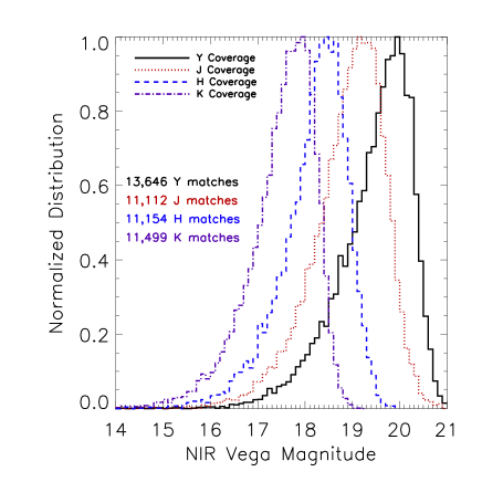
Figure 3.— Distributions of each of the four NIR bands from Stripe 82 ULAS matches in Vega magnitudes, $Y$ (solid black), $J$, (dotted red), $H$ (dashed blue) and $K$ (dot-dashed purple), for the matched objects, normalized at the peak to unity.

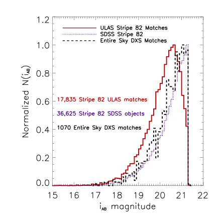
Figure 4.— Histogram showing population by $i$-band PSF magnitude. Each line was normalized to a peak value of 1.0 and a bin size of 0.1. The purple dotted line shows the histogram based on objects from R09 in Stripe 82, the solid red line displays the histogram of only ULAS matched objects and the black dashed line represents the histogram of DXS matches over the entire sky.

4.2. Magnitude Distributions

Figure 3 shows the normalized magnitude distributions for the matched objects in each of the four NIR bands, showing at which magnitude each particular band is limited by. As expected, each band peaks at a different value with shorter wavelength bands peaking at fainter magnitudes.

For Figure 4, the solid (red) histogram represents the objects which are matched in any of the 4 NIR bands, while the dotted (purple) histogram represents all the optically detected objects from the DR6pQ on Stripe 82 only. The dashed (black) line are the matches to the deeper DXS, the limiting depth of which is $K=20.8$ (Lawrence et al., 2007; Stott, 2007; Swinbank et al., 2007). Due to the smaller amount of available data for UKIDSS DXS, the matches characterized by the dashed line is less smooth than the other two histograms. The sharp cut-off at $i$=21.3 displays the $i$-band limit in the original SDSS DR6 photometric redshift catalog.

The $i$-band magnitude distribution of the matched catalog strongly suggests that the ULAS is not complete at the optically faint end of DR6pQ. The suggested completeness limit for the matched catalog is thus $i\approx 20.6$. We also caution that our matched catalog is a heterogenous sample of objects, and not a complete statistical sample as is. This will have particular ramifications when the calculation of the NIR Quasar Luminosity Function (QLF) comes to be calculated in our companion paper (Peth, Ross et al., in prep.). The significant shift between the ULAS matched histograms and the other two (optical-Stripe 82 and DXS matched) distributions most likely implies brighter optical objects are preferentially matched to ULAS NIR detections. It is reassuring to see that the DXS and optical-only histograms seem to match very well in shape and limiting magnitude, and the matched DXS catalog is provided as a test-bed for future investigations into the fainter, $i\gtrsim 20.6$ end of the $K$-band quasar population.

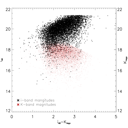
Figure 5.— Color-magnitude histograms for both the $i_{\rm AB}$ and the $K_{\rm Vega}$ bands, for $i-K$ color. Note the lack of points with faint ($i>20$) blue, $(i-K)<2.5$, colors and the effect of the limiting $K$-band magnitude for redder, $(i-K)\gtrsim 2.7$, objects.

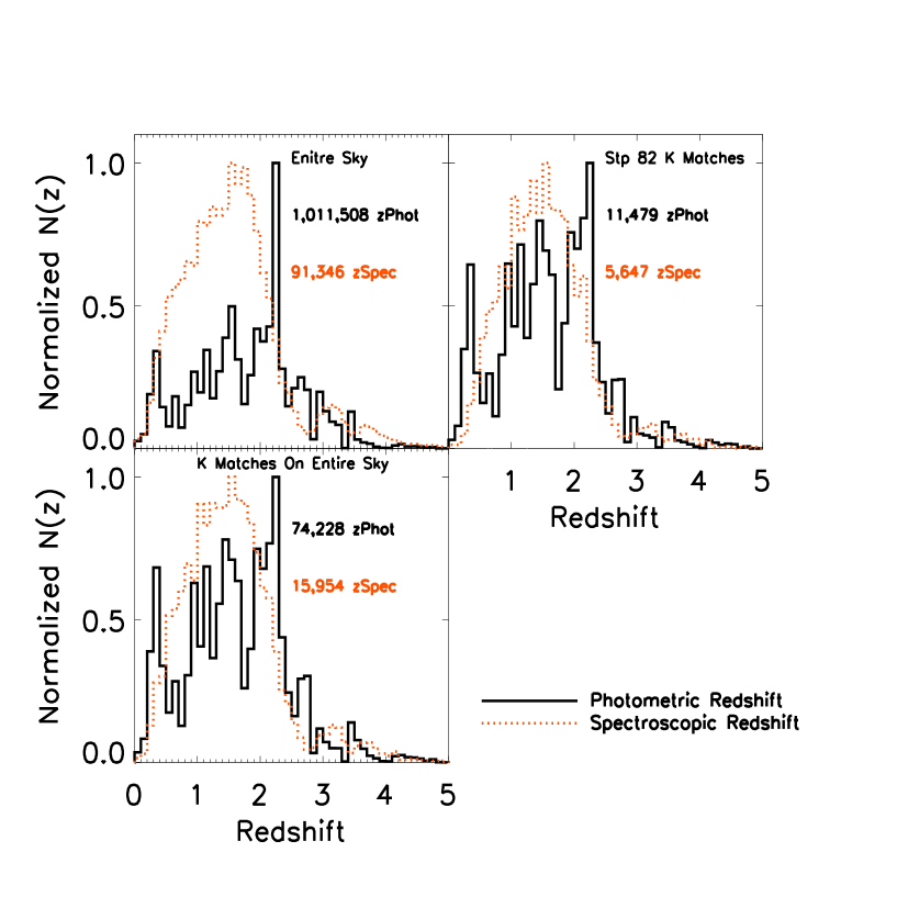
Figure 6.— Distributions of Photometric and Spectroscopic Redshifts, for the full DR6 coverage (upper left); Stripe 82 only (upper right); $K$-band matches over the DR6 (lower left). The black line represents Photometric redshift distributions and the orange line represents spectroscopic redshift distributions. The subsample of quasars from Stripe 82 (the upper-right plot) posses nearly identical redshift distributions to those over the entire sky. However, objects with $K$-band coverage have photometric redshifts that are preferentially in the low redshift bins. The difference in numbers given here and in Table 6 are due to the sample number of objects which have a photometric redshift of zPhot$=-1$.

Figure 5 gives the color-magnitude distributions for both the $i$ (black points) and $K$ (red points) bands. Again the sharp cut-off at $i=21.3$ is seen. The $K$-band limit is seen to be down to $\approx$18.4, potentially a little deeper, consistent with Figure 3. This is slightly deeper than the preliminary depths reported in Lawrence et al. (2007) but in good agreement with the updated (UKIDSS DR2) values from Warren et al. (2007) and indeed is also consistent with the measurements from the ULAS team, who give a 5$\sigma$ point source limiting magnitude of 18.27 (R.G. McMahon, priv. comm.). We suggest these faintest $K$-band objects are actually 5$\sigma$ detections in a non-$K$ NIR band, but then also have some flux in the aperture used to calculate the kAper3Mag, just possibly not to as strong a limit as the quoted 5$\sigma$ for point sources. Also apparent are the clear selection affects associated with the matched catalog, with few faint $i$-band objects at $(i-K)\lesssim 2$ and very few objects fainter than $K=18$ and redder than $(i-K)\gtrsim 3$. Again, the location of the matched catalog objects in e.g. $K$ vs. $(i-K)$ color-magnitude space, will become critical for statistical calculations using these data.

As a check, we visually examine (via the SDSS CAS Image List Tool and the UKIDSS WSA GetImage form) the very reddest objects in our catalog. These very red objects are defined as having $K$-band detections and colors of $(r-K)\geq 5.0$ or $(i-K)\geq 4.5$. There criteria return 17 and 10 objects respectively. Upon visual inspection of these 17 (10) sources, 6 (4) turned out to be either associated with, or contaminated by a foreground extended source. However, 13 out of the 17 $(r-K)$ selected objects had suspiciously high, $z=4.5-5.6$, redshifts, or zphotprob $\leq 0.8$ values, indicating the deceptive nature of these objects. Of the 10 $(i-K)$ selected sample, the 4 sources associated with the foreground galaxies, also had zphotprob $\leq 0.8$ values, while the remaining 6 objects appeared as genuine point sources. These particular very red $(i-K)$ objects deserve future follow-up investigations and we shall discuss in more detail in the next section the utility of the zphotprob flag.

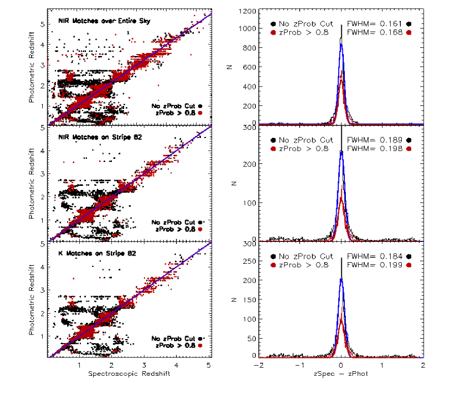
Figure 7.— Left panel: The spectroscopic redshifts plotted against photometric redshift for all matches with spectroscopic redshifts. Black points have no zphotprob cuts while red points have zphotprob$>0.8$. The 1:1 relation is plotted with a purple line. Right panel: Histograms of difference between zspec and zphot for (1) NIR matches over the entire sky (upper right); (2) NIR matches on Stripe 82 (middle right); (3) $K$- matched objects on Stripe 82 (lower right). A small full width half maximum says that the majority of photometric and spectroscopic redshifts are in agreement.

4.3. Redshift Distributions

Figure 6 shows the redshift distribution, $N(z)$, for quasars, in redshift bins of $\delta z=0.1$. Three scenarios are presented; the top left panel is for the full, optical-only, SDSS DR6 photometric redshift catalog; the lower left panel is from the matched catalog with $K$-band detections across the full coverage, and top right is from the matched catalog with $K$-band detections from Stripe 82. In each panel, the redshift distribution of the photometric redshifts is given by the solid (black) line, while those objects with spectroscopic redshifts are shown by the dashed (orange) histogram.

For the optical-only distributions the redshift distributions are potentially well matched, apart from the excess of photometric $z\sim 2.3$ objects which distort the normalization.

The redshift histograms for those objects with $K$-band detections from the matched catalogs, for both the full coverage and Stripe 82, are almost identical. Interestingly, the spike in the number of objects at $z\sim 2.3$ seems to be dramatically reduced (although does not disappear completely) for the K-band matches. As we shall see in $\S$ 4.6, when we examine the stellar contamination of our sample using the giK color-color space, we find that (i) stellar contamination is potentially higher in objects with photometric redshifts $z\sim 2.3$ and (ii) due to the respective shape of typical quasar and (e.g. M-type) stellar SEDs (e.g. Figure 1, Maddox et al., 2008), quasars will be preferentially selected over stars, if measured in the K-band. Thus, we suggest the $z\sim 2.3$ spike is because these mid-redshift objects have a lower “zphotprob” value than the general photometric quasar sample. As explained later in $\S$ 4.6 we see that the stellar locus separates nicely for $z\lesssim$ 3.2 but not for higher redshifts.

Once the $K$-band matches are made, the photometric and spectroscopic histograms now seem to be in reasonable agreement, though there are possibly decrements of photometric objects at $z\sim 0.7$ and more severely at $z\sim 1.8$. We note that this is not a new feature, having been seen in R09 (their Figure 14), and as such are motivated to continue investigations for the photometric and spectroscopic redshift distributions from our matched catalog.

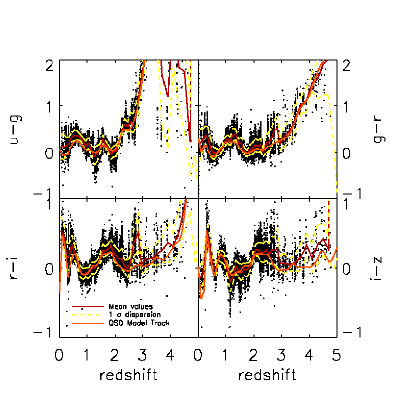
Figure 8.— Color versus redshift plots from Stripe 82 matches of $u-g$, $g-r$, $r-i$ and $i-z$. Mean magnitude ($red$ $line$) in a binsize of 0.1 mag, 1$\sigma$ dispersion ($striped$ $yellow$ $line$) both above and below the mean values, and Model Quasar colors ($orange$ $line$) as determined in (Hewett et al., 2006) are each plotted in terms of redshift.

Figure 7 shows the relationship between the photometric redshifts and the spectroscopic redshifts for the objects in our matched catalog. From top to bottom, the left panel of figure 7 is; the entire matched catalogue with spectroscopic coverage; all NIR matches on Stripe 82 and all $K$-band matches on Stripe 82. A purple line shows the 1:1 relation between spectroscopic and photometric redshifts. There is considerable structure in the photometric-spectroscopic quasar redshift relation, which again has been seen previously, e.g. Mountrichas & Shanks (2007), R09. Degeneracies between $z\sim 0.8$ and $z\sim 2.4$, as well as the width of the distributions around $z\sim 1-1.5$ can be understood by the appearance, and potential confusion of, various strong emission lines in the various (SDSS) filters (see e.g. Fan, 1999; Richards et al., 2002, 2004, for detailed descriptions). There are a couple of notable differences between the left hand panels of Figure 7 that should be briefly highlighted. First, note that a number of objects with high, $z>3$, photometric redshifts and no zphotprob cut, disappear when there is a match to the NIR data. Upon checking, we suggest this is caused by these objects generally being lower luminosity AGN than “standard” quasars, and thus thought to be at higher-$z$ than was spectroscopically found, and in general just too faint for the ULAS to detect. Also, though, this is good motivation for the utilization of the zphotprob flag. A second feature is the continued structure in the NIR matched plots. This, coupled with the general lack of structure at $z>3$, suggests that as far as photometric redshift estimation for quasars (and not e.g. differentiation between high-$z$ quasars and cool stars), then the directly matched NIR photometry, i.e. “Is there simply NIR photometry?”, actually does not provide a great amount of extra information. Of course this does not take into account the actual detected NIR fluxes (or upper limits) that would help refine photo-$z$ estimates, or the use the NIR to find very high, $z\gtrsim 6$, redshift objects.

Table 7The number of objects with photometric and spectroscopic that agree to within a 3$\sigma$ difference. The total number of objects in each bin is displayed in $italics$.

	SDSS DR6	$\%$	Stripe 82	$\%$	K-matched	$\%$
zprob $>$ 0.0	15527 (20605)	75	4933 (6589)	75	4218 (5644)	75
zprob $>$ 0.8	8981 (10188)	88	2403 (2620)	92	2114 (2292)	92

The right panel of figure 7 shows the histogram and gaussian fits with calculated full width half maxima for the difference in photometric and spectroscopic redshifts. We define that quasars with photometric and spectroscopic redshifts that have a difference greater than 3$\sigma$ to be “catastrophic failures”. All quasars with a difference in photometric and spectroscopic redshifts that fall within the 3$\sigma$ are deemed “non-catastrophic failures”. The full numbers on the agreement between spectroscopic and photometric redshifts can be seen in table 7.

Red points in the left panel of figure 7 show quasars after a redshift probability, zphotprob cut of 0.8, the value of 0.80 being inspired by the checks done by R09 (their Figure 15). This cut reduces the amount of catastrophic failure redshifts by a considerable margin, although the FWHM of the ($z$Spec-$z$phot) difference only changes very marginally. Although the zphotprob$\geq 0.80$ is a “blunt” cut, we suggest this as a relatively sensible division, but do note there are recent, more sophisticated studies, e.g. Myers et al. (2009), that show how one can take into account the full photometric redshift probability distribution function when performing statistical calculations.

4.4. Optical and NIR Colors

We now turn to the optical and NIR colors of our matched catalog.

Figure 8 shows the optical colors, $(u-g),(g-r),(r-i)$ and $(i-z)$, as a function of redshift, for our matched catalog on Stripe 82. The mean colors of the data are given by the solid (red) line, and were determined in a given bin of width $\delta z=0.1$, with the associated 1$\sigma$ standard deviations given by the striped (yellow) line. The orange triangular-pointed line represent the “Average” QSO model colors presented in Hewett et al. (2006). Hewett et al. (2006) also present “blue” and “red” model quasar spectra, where the power-law slope, $\alpha$, at wavelengths $\lambda<$12,000Å  is $\alpha=0.0,-0.6$ and $-0.3$ for blue, red and average model quasars respectively. We cut the plots at redshift $z=3$, since we feel we have poorer statistics at higher redshifts and that there are not enough points to render a representative mean value. We will examine the colors of individual high-$z$ quasars in Section 5.

Previous studies (e.g. Richards et al., 2001; Jester et al., 2005; Richards et al., 2006; Croom et al., 2009b; Hewett & Wild, 2010) have provided detailed studies of the features of quasar colors in the SDSS color space, and their form as a function of redshift. As such, we will not repeated those analyses here. Instead, we will make comparisons to the models presented in Hewett et al. (2006) of which details can be found in Maddox & Hewett (2006).

Starting with $(u-g)$, there are potentially two redshift ranges, $z=0-0.6$ and $z>2.3$ where the mean colors of the matched quasars are generally redder than the model colors. While the differences are relatively small, $\sim 0.2$ mag at the low redshift end, $\sim 0.1$ mag at the high redshifts, the model tracks are consistently bluer than the observed quasars, and at $z<0.6$, barely consistent with the 1$\sigma$ spread of the quasar $(u-g)$ color. Note also however, that care has to be taken in the determination of the $(u-g)$ color at $z>2.2$ since this is where the Lyman-$\alpha$ forest first enters the optical bands, and the determination of accurate $u$-band photometry becomes increasingly problematic.

For $(g-r)$, the model tracks reproduce the mean quasar colors well at all redshifts, $z=0-3$. However, there might be a tend for the observed quasars to be generally redder at low ($z<0.5$) and high ($z>2.3$) redshift, though this can be seen as marginal.

For $(r-i)$, it appears that the model tracks do in fact reproduce the mean quasar colors very well, for $z<2$, and especially for $z=0.7-2.0$. The disagreement between model and observed mean at $z\approx 0.5$ seems to be caused by the fact that there are a noticeable number of (red and blue) outliers, with the observed colors of the general population better tracked. As can be seen, the model colors agree well with the raw data at $z\approx 0.5$, $(r-i)\sim-0.1$. The model tracks begin to struggle to reproduce the observed colors at $z>2$, but remain consistent with the 1$\sigma$ dispersion until $z>2.5$.

For $(i-z)$, just as for $(r-i)$, the model tracks replicate the mean colors very closely, all the way to $z\sim 2.7$ and thus for the optical colors, the models perform best for these reddest bands. At $z>2.7$ for $(i-z)$ and indeed all four optical colors, the models struggle to reproduce the observed quasar colors at these higher redshifts, consistently being too blue.

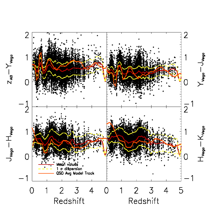
Figure 9.— Color versus redshift plots from Stripe 82 matches. $z-Y$ (top left); $Y-J$ (top right); $J-H$ (bottom left) and $H-K$ (bottom right). The given lines are the same as in Figure 8. Note the dip and rise at $z\sim 0.4,\sim 0.7,\sim 0.9$ and $\sim 1.3$, for $z-Y$, $Y-J$, $J-H$ and $H-K$ respectively, due to the location of the strong H$\alpha$ emission line in the NIR filters.

We tentatively suggest this is the same affect as has recently been reported in Prochaska et al. (2009) and Worseck & Prochaska (2010), namely, that the original SDSS color-selection that was used to select quasars, and from which the R09 and hence our own matched catalog is based, may be systematically biased as these redshifts. It has long been known that the redshifts around $z\sim 2.7$ are very troublesome for selecting quasars, since the broadband colors are so similar to those of e.g. F5 V stars (see e.g. Figure 1 of Fan, 1999), leading to very poor survey efficiency and heavy incompleteness (Richards et al., 2006; Croom et al., 2009b). However, these recently analyses model in great detail the spectra of these high redshift objects, paying particular attention to the flux transmission (and decrement) blueward of Lyman-$\alpha$, in order to generate accurate mock UV and optical photometry. Specifically, Worseck & Prochaska (2010) suggest that the SDSS color-selection selection systematically misses quasars with blue, $u-g\lesssim 2$ colors at $3\lesssim z\lesssim 3.5$ due to the preference of selecting $z\gtrsim 2.7$ quasars with intervening H I Lyman limit systems (which generally turn quasars red). This would potentially begin to explain the offset between the model tracks and observed quasar colors in Figure 8. We are keen to note however, that there are more recent versions of the quasar color models given in Hewett et al. (2006) and that further analysis is required here.

Noting the shape, response and wavelength coverage (and indeed gaps between filters, see e.g. Figure 1 Hewett et al., 2006) between the $Y$, $J$, $H$ and $K$ filters, we can now begin to explain the NIR color trends with redshift seen in Figure 9. The NIR color-redshift relations still exhibit structure, but arguably less than in the optical. This is mainly due to the fact that it is now the lines towards the redder end of the optical, and in particular H$\alpha$, that lead to the trends seen in Figure 9. We note that Assef et al. (2010) and in particular Glikman et al. (2006, their table 6) are useful references for the following.

The H$\alpha$ line is very much the dominant emission line over the rest-wavelength range, $\lambda=6500-21000$Å. The blended He I and Paschen-$\gamma$ lines at around 10,900Å, the Paschen-$\beta$ line at 12,820Å, and Paschen-$\alpha$ emission at 18,756Å, are also present but contribute little. For example, even if a Paschen line had an equivalent width of 100Å, with the NIR bands being so broad (e.g. $\approx 4000$Å  for the K-band; see Table LABEL:tab:filter_details), the contribution here would be $\sim$a few % at redshift $z=0$ - significantly smaller than the measurement errors in the colors. These emission lines are superimposed on the continuum power-law spectrum, $F({\nu})\propto\nu^{\alpha}$ where $\alpha=-0.78$, measured over $\lambda=5700-10850$Å  (Glikman et al., 2006, but see also Kishimoto et al. (2008)).

Thus, starting with the top left panel, $(z-Y)$, we note the dip at redshift $z\sim 0.3$ is due to H$\alpha$ entering the $z$-band causing the general quasar color to be blue, while at redshift, $z\sim 0.45$, H$\alpha$ is leaving $z$, and entering the $Y$-band causing the colors to become redder, reaching an observed mean (model) peak of $(z-Y)\approx 0.5$ (1.0) at redshift $z\approx 0.6$. At $z\sim 0.7$, H$\alpha$ leaves the $Y$-band. The model tracks trace the observed colors well up to $z\sim 2$, but then grow progressively redder and redder at higher redshifts (though do remain within the measured 1$\sigma$ dispersion). This behavior, the model tracks being redder than the observed quasar colors at high, $z>2$, redshift is only see in $(z-Y)$.

Moving to, $(Y-J)$, we again see a dip, at $z\sim 0.5$, towards bluer colors, as H$\alpha$ enters the $Y$-band, and then a rise towards redder colors, peaking at redshift $z\sim 0.9$ as H$\alpha$ moves out of $Y$, and into the $J$-band (noting the gap between bands at 1.4$\mu$m). The models’ continued rise and fall behavior at $z\sim 1.1-2.1$ can be explained by H$\beta$, then O III and then Mg II marching through the WFCAM bands. The observed mean colors however, show a much smaller amplitude of color-change over this redshift range, though the individual objects seem to respond more to these emission lines.

For $(J-H)$, the passing of H$\alpha$ first through the $J$-band and then through the $H$-band gives the trough at $z\sim 0.8-1.1$. Here the model tracks, even out to our maximum plotted redshift of $z=3$, replicate the observed quasar colors very well. The success of the model tracks in $(J-H)$ could potentially be used for quasar selection in future redshift surveys, including the implementation of “KX” completeness tests (Croom et al., 2001; Smail et al., 2008; Jurek et al., 2008).

Finally, for $(H-K)$, the H$\alpha$ trough is across redshifts $z=1.2-1.8$. Note the broadening of the trough in the four NIR colors as H$\alpha$ passes to higher redshifts. Again the model tracks replicate the observed quasar colors well, though there is a large dispersion at all redshifts. The one place the models tracks are in disagreement is at low, $z<0.5$, redshifts. This is potentially due to flux from an underlying red host galaxy being over-represented, but more likely, the lack of data points to calculate the observed mean well.

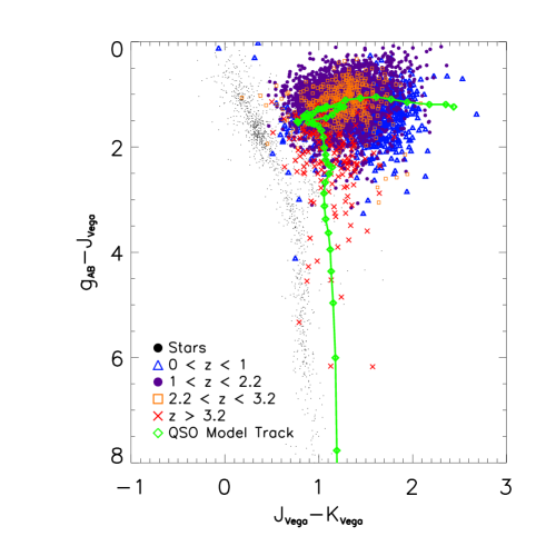
Figure 10.— The location of matched quasars, and stellar sources in the $g-J$ vs. $J-K$ plane. Stars are solid (black) points; $0<z<1$ quasars are open (blue) triangles; $1<z<2.2$ quasars are solid (purple) circles; $2.2<z<3.2$ quasars are open (orange) squares and (red) crosses are $z>3.2$ objects. The (“average”) model tracks of Hewett et al. (2006) are given by the (green) line, with $z=0$ around $(J-K)=2.5$ increasing in $\Delta z=0.1$ steps (green diamonds) to $z=4.8$ at $(g-J)=8$.

4.5. Stellar Contamination

Following Maddox et al. (2008) and Smail et al. (2008), we now investigate the location in $(g-J)$ vs. $(J-K)$ (“$gJK$”) color-space of our matched catalog.

Here our motivation is not so much directed at creating complete “KX” selected samples, but is more towards determining if there is a certain part of color-space where quasars, and in particular mid, $z=2.2-3.5$, redshift quasars lie apart from stars. This is of key importance to two new spectroscopic surveys, the SDSS-III: Baryon Oscillation Spectroscopic Survey (BOSS; Schlegel et al., 2007) and the AAT-UKIDSS-SDSS (AUS) QSO Survey (P.I. S.M. Croom). Both the BOSS and AUS survey aim to gather spectroscopic information for $z>2.2$ quasars, for investigations into cosmological parameters using the Lyman-$\alpha$ forest (BOSS) and global quasar population studies (AUS and BOSS). As such, any technique to reduce stellar contamination is of upmost interest to these survey teams. The KX technique is based upon the fact that at redshifts $z\approx=2-3$, NIR photometry samples the Rayleigh-Jeans tails of A and F stars (the major contaminants in an optical-based quasar selection), where flux is decreasing rapidly with the increasing wavelength, whereas quasar SEDs are remaining relatively flat.

In Figure 10 we plot the $(g-J)$ vs. $(J-K)$ colors for the objects on Stripe 82 from our match catalog, with spectroscopic redshifts. We also select 5000 point sources lying on Stripe 82, from the SDSS CAS, with spectroscopic redshifts less than 0.02, and gather ULAS NIR photometry for these objects where available. These can be considered stars because of their low redshifts and morphology, and are solid (black) points in $gJK$ figure. $0<z<1$ quasars are open (blue) triangles; $1<z<2.2$ quasars are solid (purple) circles; $2.2<z<3.2$ quasars are open (orange) squares and (red) crosses are $z>3.2$ objects. Again we show the “Average” model tracks of Hewett et al. (2006), given by the (green) line, with $z=0$ around $(J-K)=2.5$ increasing in $\Delta z=0.1$ steps (green diamonds) to $z=4.8$ at $(g-J)=8$.

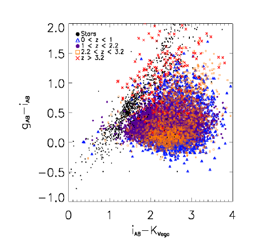
Figure 11.— $g-i$ vs. $i-K$ diagram to show the colors of Stripe 82 objects from the matched catalog. Stars are solid (orange) points. Quasars are displayed in bins of varying redshift ranges: $z<1.0$, black stars; $1.0<z<2.2$ blue open triangles; $2.2<z<3.2$ orange open squares, and greater than 3.2, red crosses.

Our results are qualitatively very similar to that of Maddox et al. (2008), that is, (a) the stellar locus traces out a clear band in $gJK$ color-space, related to the different stellar spectral type and (b) that in general, stars appear to have $gJK$ colors that are in a distinct region of color space than quasars, especially those with $2.2<z<3.2$ (orange) open squares in Figure 10. We find this very encouraging and suggest that selection in the $gJK$ color-plane could be of good utility to the BOSS and AUS surveys. We also note the almost complete lack of quasars in our $gJK$ plot that have colors similar to those of (model) galaxies around $(J-K)\approx 1.7$ and $(g-J)\approx 4.5$. However, a strong caveat that has to be imposed here is to recall that the original R09 quasar selection was predominantly geared towards $z<2$ “UVX” selected, non-extended objects. This is to be compared with the study by Smail et al. (2008) who find that lower, $z\sim 0.45$ compact galaxies are the main and major contaminent of their “KX” selection. Interestingly, Smail et al. (2008) report that the spectral mix of the contaminating population includes sources whose spectra are best fit by both broadline and narrow-line AGN templates, as well as narrow emission-line, absorption-line and spiral galaxy templates. Indeed, early analysis from the BOSS (Ross et al., 2010, in prep.) suggests that these morphologically compact, narrow-emission line galaxies at lower, $z\approx 0.2-0.5$ redshift, continue to be selected as $z>2.2$ quasars.

Inspired by Mehta et al. (2010), we also plot the location of Stripe 82 objects from the matched catalog, this time in $g-i$ vs. $i-K$ ($giK$) color-space, see Figure 11. Again, quasars are displayed in bins of varying redshift ranges: $z<1.0$, black stars; $1.0<z<2.2$ blue open triangles; $2.2<z<3.2$ orange open squares, and greater than 3.2, red crosses. On initial inspection, we again see the stellar locus inhabiting a distinct sequence in color-space, which is somewhat separate to that of the quasars. However, we leave further investigations into the use of the $(g-i)$ vs. $(i-K)$ color-space for star-quasar-galaxy identification, and survey completeness to future study.

5. High Redshift Quasars

5.1. High Redshift objects in Matched Catalog

Figure 12 plots high-redshift quasars, those with $z\gtrsim 4.6$ (essentially $r$-band drop-outs), in $iYJ$ color-color space. Only objects with both a “good” photometric and spectroscopic redshifts are plotted. For a photometric redshift to be considered “good” it must be within the error limits of the spectroscopic redshift. Out of 49 high-redshift ($z\gtrsim 4.6$) quasars possessing both a photometric and spectroscopic redshift, 40 have “good” photometric redshifts. Out of this group of 40 quasars, 23 objects possess both $Y$ and $J$ magnitudes, and we plot these in Figure 12. These objects span the redshift range of $4.606\leq z_{\rm spec}\leq 5.289$. No obvious trends are visible, arguably due to our small sample size. However, we can say that these high-redshift quasars have roughly the same color and follow the given high-$z$ model tracks of Hewett et al. (2006) well.

5.2. Very High Redshift objects

Table 8Photometric properties of 6 very high $z>5.7$, redshift quasars as detected in the ULAS DR3, along with their spectroscopic redshifts. Positions are in degrees and J2000 coordinates. References: ^aVenemans et al. (2007). ^bJiang et al. (2008). ^cFan et al. (2006). ^dMortlock et al. (2009).

R.A.	Decl.	redshift	$u$	$g$	$r$	$i$	$z$	$Y$	$J$	$H$	$K$
a,b30.8849	0.2081	5.850$\pm$0.003	–	–	–	23.72$\pm$0.22	20.87$\pm$0.10	19.85$\pm$0.12	19.06$\pm$0.10	17.76$\pm$0.07	17.32$\pm$0.09
b58.45719	1.0680	6.049$\pm$0.004	–	–	–	24.03$\pm$0.30	20.54$\pm$0.08	20.12$\pm$0.16	19.46$\pm$0.16	18.55$\pm$0.17	18.16$\pm$0.22
c129.1827	0.9148	5.82$\pm$0.02	26.21$\pm$0.57	25.80$\pm$0.55	22.75$\pm$0.23	21.23$\pm$0.09	18.86$\pm$0.05	18.26$\pm$0.03	17.70$\pm$0.029	17.03$\pm$0.03	16.19$\pm$0.03
d199.7970	9.8476	6.127$\pm$0.004	–	–	–	22.55$\pm$0.09	19.99$\pm$0.03	19.22$\pm$0.06	18.69$\pm$0.05	–	17.55$\pm$0.08
c212.7970	12.2937	5.93$\pm$0.02	24.77$\pm$0.99	24.79$\pm$0.71	23.22$\pm$0.28	22.86$\pm$0.30	19.65$\pm$0.08	19.47$\pm$0.07	19.22$\pm$0.093	18.29$\pm$0.09	17.46$\pm$0.08
c245.8826	31.2001	6.22$\pm$0.02	23.96$\pm$0.91	25.44$\pm$0.62	24.88$\pm$ 0.58	24.50$\pm$0.62	20.07$\pm$0.10	–	19.17$\pm$0.111	–	–

For our final investigations, we actually leave the matched quasar catalog, and concentrate solely on the ULAS DR3 to investigate the NIR photometric properties of the very high, $z>5.7$, redshift objects that are given in the series of Fan et al., and Jiang et al. papers papers, (Fan et al., 2006; Jiang et al., 2008, 2009, respectively and references therein). We also note the 19 very high redshift quasars discovered by the Canada-France High-$z$ Quasar Survey (CFHQS; Willott et al., 2007, 2009, 2010). However, the CFHQS is not covered by the ULAS DR3, and only has the one ($J$) out of the 4 ULAS bands, so the NIR properties of these objects are not reported here.

Out the 30 objects - 19 from the Fan et al. studies, 11 from Jiang et al. with one object in common and the additional object from Mortlock et al. (2009), 13 (12) are within the ULAS DR3 ($K$-band) footprint, and 6 were detected in one or more of the ULAS bands. The photometric properties of these 6 detections, along with their spectroscopic redshifts, are given in Table LABEL:tab:fan. 5 of the 6 objects have $K$-band detections, with magnitudes ranging from $K=16.19-18.16$. The reason for only $5/12$ having $K$-band detections we suggest is primarily due to the limiting magnitude for the ULAS. As a quick check, we note that the Jiang et al. objects were discovered using the deeper SDSS optical imaging, this means, potentially 6 out of the 7 $K$-band non-detections are fainter than the ULAS $K$-band limit. The mean $J$-band magnitude from the 6 objects presented in Jiang et al. (2009) is $J\approx 21.0\pm 0.2$, whereas for the objects in Table LABEL:tab:fan it is $J\approx 18.9\pm 0.3$. Thus if the colors of these $z\sim 6$ objects are $(J-K)\sim 1.1-1.8$, even the brightest and reddest object in Jiang et al. (2009) would be right on the ULAS $K$-band limit, with the average object being closer to $K=19.3$.

Our results are generally consistent with Venemans et al. (2007) who report the discovery of the quasar at $z=5.85$ (designated ULAS J020332.38+001229.2) after analysis of 106 deg² of sky from UKIDSS DR1, and Mortlock et al. (2009) who report the discovery of ULAS J1319+0950, a quasar at $z=6.13$. Glikman et al. (2008) surveyed 27.3 deg² of the ULAS EDR, but found no $z>6$ objects from spectroscopy of a 34 candidate list.

Deeper and more complete surveys will be needed to get a better estimate on the spatial density of high-redshift quasars. To this affect, the Visible and Infrared Survey Telescope for Astronomy (VISTA; Emerson et al., 2004; Emerson & Sutherland, 2010) has recently been commissioned, and is currently ramping up its suite of six imaging surveys (Arnaboldi et al., 2010). Of direct interest to the high redshift Universe will be the “VISTA Hemisphere Survey”, (VHS; PI: R.G. McMahon), which aims to image the entire $\sim$20 000deg² Southern Sky, down to $J_{\rm AB}=21.2$ and $Ks_{\rm AB}=20.0$ ($J\approx 20.3$ and $K\approx 18.1$). On a longer timescale, the Synoptic All-Sky Infrared (SASIR; Bloom et al., 2009) is planned. The hope and goals of these surveys will be to find 100’s (VISTA) or potentially 1000’s (SASIR) of $z>6$ quasars. Whether these numbers are borne out in the new observations, will, of course, be of great future interest.

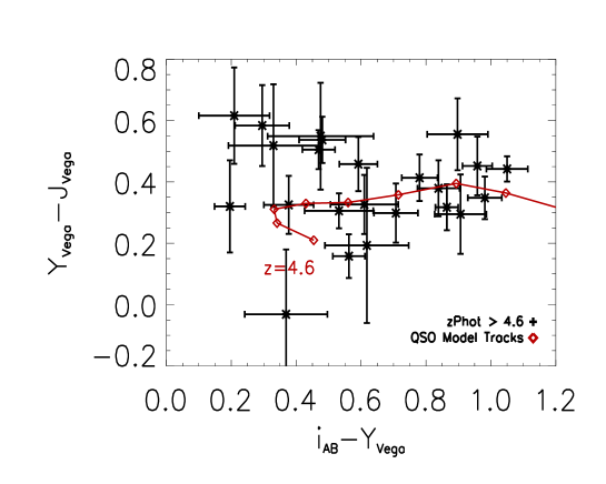
Figure 12.— High, $4.6<z<5.35$ redshift quasars in $i-Y$ vs $Y-J$ color space. The “average” quasar model tracks of Hewett et al. (2006) are again given, starting at $z=4.6$ (labelled) and then increasing in $\Delta z=0.1$ steps, shown by the open (red) diamonds.

6. Conclusions

We have matched the optical, photometrically selected quasar catalog of R09 to detections from the ULAS DR3. The positions of the 1,015,082 objects from the DR6pQ catalog were uploaded to the WFCAM Science Archive. To count as a match, the returned NIR object must have been the closest object in the ULAS to the SDSS coordinates, selected from within a pairing radius of 1^′′. As long as at least 1 NIR band contained a non-default, i.e. not -9.9999$\times 10^{8}$ value, the object was considered a good match.

Our final catalog has 130,827 objects with detections in the optical and one or more NIR bands; of which 74,351 objects have K-band detections and 42,133 objects have the full 9-band photometry. Using this matched catalog, we present the following main conclusions:

• The positional standard deviation of the SDSS Quasar to ULAS matches is $\delta_{\rm R.A.}=0.1370^{\prime\prime}$ and $\delta_{\rm Decl.}=0.1314^{\prime\prime}$. We find an absolute systematic astrometric offset between the SDSS Quasar catalog and the ULAS, of $|{\rm R.A._{offset}}|=0.025^{\prime\prime}$, and $|{\rm Decl._{offset}}|=0.040^{\prime\prime}$; we suggest the nature of this offset to be due to the matching of catalogs, rather than image level data.

• Our matched catalog has a surface density of $\sim$108 deg^-2, for objects detected in any of the four NIR bands, and $\approx 53$ deg^-2 for objects $K\leq 18.27$. This compares to the $\approx 122$ deg^-2 found from the R09 DR6pQ catalog and $85-150$ deg^-2 down to $K\leq 20$ from Smail et al. (2008).

• Tests using our matched catalog, along with data from the UKIDSS DXS, implies that our limiting magnitude is $i\approx 20.6$ and that the reddest, $(r-K)\geq 5.0$ objects turn out to be either associated with, or contaminated by, a foreground extended source.

• We plot redshift histograms for the Stripe 82 subsample, $K$-matches sample and total matched sample. The photometric $N(z\sim 2.3)$ spike seen for the “total sky” sample appears to be dramatically reduced (although does not disappear completely) for the K-band matches. The photometric and spectroscopic histograms now seem to be in reasonable agreement, though there are possible deficiencies of photometric objects at $z\sim 0.7$ and in particular, $z\sim 1.9$.

• Color-redshift diagrams, for the optical and NIR, show the close agreement between our matched catalog and the “average” models of Hewett et al. (2006), at redshift $z\lesssim 2.0$. At higher redshifts, the models generally appear to be generally bluer than the mean observed quasar colors. We tentatively suggest this is the same affect as has recently been reported in Worseck & Prochaska (2010), namely, that the original SDSS color-selection that was used to select quasars (and ultimately our own matched catalog) may be systematically biased towards missing blue $(u-g)\leq 2.0$ quasars at $z\sim 2.2-3.5$, due to the selection preferentially selecting intervening H I Lyman limit systems.

• Since stellar contamination is of great interest for ongoing quasar surveys such as the SDSS-III:BOSS and AUS, we plot a test set of stellar data with our matched catalog data in $gJK$ and $giK$ color space. We confirm findings from previous studies, in particular Maddox et al. (2008), that $(a)$ the stellar locus traces out a clear band in $gJK$ color-space, related to the different stellar spectral type and $(b$ that in general, quasars, especially those with $2.2<z<3.2$ mostly lie in a distinct region of $gJK$ color space than stars.

• We plot the $iYJ$ colors of our matched catalog for high, $z>4.6$, redshift spectroscopically confirmed quasars, again comparing to model tracks, though no obvious trends are seen. Finally, just using the ULAS DR3 and the very high, $z>5.7$, redshift objects reported in Fan et al. (2006), Jiang et al. (2008), Jiang et al. (2009) and Mortlock et al. (2009), we find 6 (5) out of 13 (12) quasars have NIR ($K$) band detections.

It is worthwhile to mention that many of our tests have also been performed very recently in Wu & Jia (2010), and although we have not performed any direct comparisons between the results found herein and their study, we see very good general agreement, e.g. for color-$z$ relations, between the two investigations.

The major motivation for the construction of the matched catalog presented here, was its utilization in a future study where we measure the $K$-band quasar luminosity function. As quasars are measured further in the NIR, the flux due to host galaxies is no longer negligible but will rather constitute a sizeable percentage of the total bolometric flux from a quasar. Our future work (Peth, Ross et al. in prep.), will address this, and other issues in order to construct and measure the observed $K$-band quasar luminosity function.

Advancement can come from technological breakthroughs as well as new theoretical insights. Future telescopes and surveys, e.g. VISTA-VHS and the SASIR, will not only cover more of the sky but should also be able to observe to greater depths. Future observations will warrant an updated analysis of quasar properties in multiple bands, and will be both necessary and essential to further understand the formation and evolution of quasars.

Appendix A A. Photometric Bands and Conversions

Due to the differing normalizations between the SDSS and UKIDSS photometric systems, certain corrections are required. To present our data in the purest sense, all the NIR magnitudes from UKIDSS (originally AB magnitudes) were corrected to Vega magnitudes as suggested in Hewett et al. (2006).

Although ULAS magnitudes are reported in terms of Vega and SDSS magnitudes are reported in AB terms for the most part whenever an optical-NIR color was calculated both magnitudes were left in their default term.

Table 9Adapted from Table 19 of Stoughton et al. (2002), Table 1 of Lawrence et al. (2007) and Table 7 of Hewett et al. (2006).

Band	$\lambda_{\rm eff}{\buildrel{}_{\circ}\over{\mathrm{A}}}$	$\lambda_{\rm min}{\buildrel{}_{\circ}\over{\mathrm{A}}}$	$\lambda_{\rm max}{\buildrel{}_{\circ}\over{\mathrm{A}}}$	FWHM ${\buildrel{}_{\circ}\over{\mathrm{A}}}$	AB - Vega Transformations
u	3551	3005	4000	581	$u$ = $u_{AB}$ - 0.927
g	4686	3720	5680	1262	$g$ = $g_{AB}$ + 0.103
r	6166	5370	7120	1149	$r$ = $r_{AB}$ - 0.146
i	7480	6770	8380	1237	$i$ = $i_{AB}$ - 0.366
z	8932	8000	10620	994	$z$ = $z_{AB}$ - 0.533
Y	10305	9790	10810	1020	$Y$ = $Y_{AB}$ - 0.634
J	12483	11690	13280	1590	$J$ = $J_{AB}$- 0.938
H	16313	14920	17840	2920	$H$ = $H_{AB}$ - 1.379
K	22010	20290	23800	3510	$K$ = $K_{AB}$ - 1.9

References

- Abazajian et al. (2009) Abazajian K. N., et al., 2009, ApJS, 182, 543
- Adelman-McCarthy et al. (2008) Adelman-McCarthy J. K., et al., 2008, ApJS, 175, 297
- Arnaboldi et al. (2010) Arnaboldi M., et al., 2010, The Messenger, 139, 6
- Assef et al. (2010) Assef R. J., et al., 2010, ApJ, 713, 970
- Ball et al. (2007) Ball N. M., Brunner R. J., Myers A. D., Strand N. E., Alberts S. L., Tcheng D., Llorà X., 2007, ApJ, 663, 774
- Barkhouse & Hall (2001) Barkhouse W. A., Hall P. B., 2001, AJ, 121, 2843
- Bloom et al. (2009) Bloom J. S., et al., 2009, arXiv:0905.1965v2
- Casali et al. (2007) Casali M., et al., 2007, Astron. & Astrophys., 467, 777
- Chiu et al. (2007) Chiu K., Richards G. T., Hewett P. C., Maddox N., 2007, MNRAS, 375, 1180
- Croom et al. (2009a) Croom S. M., et al., 2009a, MNRAS, 399, 1755
- Croom et al. (2009b) Croom S. M., et al., 2009b, MNRAS, 392, 19
- Croom et al. (2004) Croom S. M., Smith R. J., Boyle B. J., Shanks T., Miller L., Outram P. J., Loaring N. S., 2004, MNRAS, 349, 1397
- Croom et al. (2001) Croom S. M., Warren S. J., Glazebrook K., 2001, MNRAS, 328, 150
- Cutri et al. (2002) Cutri R. M., Nelson B. O., Francis P. J., Smith P. S., 2002, in 284 A. C. S., ed., Green, R. F., Khachikian, E. Y. and Sanders, D. B. The 2MASS Red AGN Survey. p. 127
- Dye et al. (2006) Dye S., et al., 2006, MNRAS, 372, 1227
- Efstathiou & Rowan-Robinson (1995) Efstathiou A., Rowan-Robinson M., 1995, MNRAS, 273, 649
- Emerson & Sutherland (2010) Emerson J., Sutherland W., 2010, The Messenger, 139, 2
- Emerson et al. (2004) Emerson J. P., Sutherland W. J., McPherson A. M., Craig S. C., Dalton G. B., Ward A. K., 2004, The Messenger, 117, 27
- Fan (1999) Fan X., 1999, AJ, 117, 2528
- Fan et al. (2001) Fan X., et al., 2001, AJ, 121, 54
- Fan et al. (2006) Fan X., et al., 2006, AJ, 132, 117
- Francis et al. (2004) Francis P. J., Nelson B. O., Cutri R. M., 2004, AJ, 127, 646
- Fukugita et al. (1996) Fukugita M., Ichikawa T., Gunn J. E., Doi M., Shimasaku K., Schneider D. P., 1996, AJ, 111, 1748
- Glikman et al. (2008) Glikman E., Eigenbrod A., Djorgovski S. G., Meylan G., Thompson D., Mahabal A., Courbin F., 2008, AJ, 136, 954
- Glikman et al. (2006) Glikman E., Helfand D. J., White R. L., 2006, ApJ, 640, 579
- Glikman et al. (2007) Glikman E., Helfand D. J., White R. L., Becker R. H., Gregg M. D., Lacy M., 2007, ApJ, 667, 673
- Hambly et al. (2008) Hambly N. C., et al., 2008, MNRAS, 384, 637
- Hewett et al. (2006) Hewett P. C., Warren S. J., Leggett S. K., Hodgkin S. T., 2006, MNRAS, 367, 454
- Hewett & Wild (2010) Hewett P. C., Wild V., 2010, MNRAS, 405, 2302
- Hodgkin et al. (2009) Hodgkin S. T., Irwin M. J., Hewett P. C., Warren S. J., 2009, MNRAS, 394, 675
- Jester et al. (2005) Jester S., et al., 2005, AJ, 130, 873
- Jiang et al. (2006) Jiang L., et al., 2006, AJ, 131, 2788
- Jiang et al. (2008) Jiang L., et al., 2008, AJ, 135, 1057
- Jiang et al. (2009) Jiang L., et al., 2009, AJ, 138, 305
- Jurek et al. (2008) Jurek R. J., Drinkwater M. J., Francis P. J., Pimbblet K. A., 2008, MNRAS, 383, 673
- Kishimoto et al. (2008) Kishimoto M., Antonucci R., Blaes O., Lawrence A., Boisson C., Albrecht M., Leipski C., 2008, Nature, 454, 492
- Kouzuma & Yamaoka (2010a) Kouzuma S., Yamaoka H., 2010a, Astron. & Astrophys., 509, A64
- Kouzuma & Yamaoka (2010b) Kouzuma S., Yamaoka H., 2010b, MNRAS, 405, 2062
- Lacy et al. (2004) Lacy M., et al., 2004, ApJS, 154, 166
- Lawrence et al. (2007) Lawrence A., et al., 2007, MNRAS, 379, 1599
- Maddox & Hewett (2006) Maddox N., Hewett P. C., 2006, MNRAS, 367, 717
- Maddox et al. (2008) Maddox N., Hewett P. C., Warren S. J., Croom S. M., 2008, MNRAS, 386, 1605
- Martin et al. (2005) Martin D. C., et al., 2005, ApJ Lett., 619, L1
- Mehta et al. (2010) Mehta S. S., Mahon R. G., Richards G. T., Hewett P. C., 2010 Vol. 41 of BAAS, Optical+NIR Quasar Selection with the SDSS and UKIDSS. p. 373
- Mortlock et al. (2009) Mortlock D. J., et al., 2009, Astron. & Astrophys., 505, 97
- Mountrichas & Shanks (2007) Mountrichas G., Shanks T., 2007, MNRAS, 380, 113
- Myers et al. (2007) Myers A. D., Brunner R. J., Nichol R. C., Richards G. T., Schneider D. P., Bahcall N. A., 2007, ApJ, 658, 85
- Myers et al. (2006) Myers A. D., et al., 2006, ApJ, 638, 622
- Myers et al. (2009) Myers A. D., White M., Ball N. M., 2009, MNRAS, 399, 2279
- Nakos et al. (2009) Nakos T., et al., 2009, Astron. & Astrophys., 494, 579
- Ofek et al. (2007) Ofek E. O., Oguri M., Jackson N., Inada N., Kayo I., 2007, VizieR Online Data Catalog, 838, 20412
- Oke & Gunn (1983) Oke J. B., Gunn J. E., 1983, ApJ, 266, 713
- Padmanabhan et al. (2008) Padmanabhan N., et al., 2008, ApJ, 674, 1217
- Pier & Krolik (1993) Pier E. A., Krolik J. H., 1993, ApJ, 418, 673
- Prochaska et al. (2009) Prochaska J. X., Worseck G., O’Meara J. M., 2009, ApJ Lett., 705, L113
- Richards et al. (2001) Richards G. T., et al., 2001, AJ, 122, 1151
- Richards et al. (2002) Richards G. T., et al., 2002, AJ, 123, 2945
- Richards et al. (2004) Richards G. T., et al., 2004, ApJS, 155, 257
- Richards et al. (2006) Richards G. T., et al., 2006, AJ, 131, 2766
- Richards et al. (2009a) Richards G. T., et al., 2009a, ApJS, 180, 67
- Richards et al. (2009b) Richards G. T., et al., 2009b, AJ, 137, 3884
- Ross et al. (2009) Ross N. P., et al., 2009, ApJ, 697, 1634
- Sánchez et al. (2006) Sánchez A. G., Baugh C. M., Percival W. J., Peacock J. A., Padilla N. D., Cole S., Frenk C. S., Norberg P., 2006, MNRAS, 366, 189
- Sanders et al. (1989) Sanders D. B., Phinney E. S., Neugebauer G., Soifer B. T., Matthews K., 1989, ApJ, 347, 29
- Schlegel et al. (2007) Schlegel D. J., et al., 2007, in BAAS Vol. 38, SDSS-III: The Baryon Oscillation Spectroscopic Survey (BOSS). p. 966
- Schlegel et al. (1998) Schlegel D. J., Finkbeiner D. P., Davis M., 1998, ApJ, 500, 525
- Schneider et al. (2007) Schneider D. P., et al., 2007, AJ, 134, 102
- Schneider et al. (2010) Schneider D. P., et al., 2010, AJ, 139, 2360
- Shakura & Sunyaev (1973) Shakura N. I., Sunyaev R. A., 1973, Astron. & Astrophys., 24, 337
- Sharp et al. (2002) Sharp R. G., Sabbey C. N., Vivas A. K., Oemler A., McMahon R. G., Hodgkin S. T., Coppi P. S., 2002, MNRAS, 337, 1153
- Shen et al. (2007) Shen Y., et al., 2007, AJ, 133, 2222
- Shen et al. (2009) Shen Y., et al., 2009, ApJ, 697, 1656
- Skrutskie et al. (2006) Skrutskie M. F., et al., 2006, AJ, 131, 1163
- Smail et al. (2008) Smail I., et al., 2008, MNRAS, 389, 407
- Souchay et al. (2009) Souchay J., et al., 2009, Astron. & Astrophys., 494, 799
- Spergel et al. (2007) Spergel D. N., et al., 2007, ApJS, 170, 377
- Stott (2007) Stott J. P., 2007, PhD thesis, Durham University
- Stoughton et al. (2002) Stoughton C., et al., 2002, AJ, 123, 485
- Swinbank et al. (2007) Swinbank A. M., et al., 2007, MNRAS, 379, 1343
- Trammell et al. (2007) Trammell G. B., Vanden Berk D. E., Schneider D. P., Richards G. T., Hall P. B., Anderson S. F., Brinkmann J., 2007, AJ, 133, 1780
- Vanden Berk et al. (2005) Vanden Berk D. E., et al., 2005, AJ, 129, 2047
- Venemans et al. (2007) Venemans B. P., McMahon R. G., Warren S. J., Gonzalez-Solares E. A., Hewett P. C., Mortlock D. J., Dye S., Sharp R. G., 2007, MNRAS, 376, L76
- Warren et al. (2007) Warren S. J., et al., 2007, arXiv:astro-ph/0703037v3
- Warren et al. (2000) Warren S. J., Hewett P. C., Foltz C. B., 2000, MNRAS, 312, 827
- Weinstein et al. (2004) Weinstein M. A., et al., 2004, ApJS, 155, 243
- Willott et al. (2007) Willott C. J., et al., 2007, AJ, 134, 2435
- Willott et al. (2009) Willott C. J., et al., 2009, AJ, 137, 3541
- Willott et al. (2010) Willott C. J., et al., 2010, AJ, 139, 906
- Wolf et al. (2003) Wolf C., Wisotzki L., Borch A., Dye S., Kleinheinrich M., Meisenheimer K., 2003, Astron. & Astrophys., 408, 499
- Worseck & Prochaska (2010) Worseck G., Prochaska J. X., 2010, ArXiv e-prints
- Wright (2006) Wright E. L., 2006, PASP, 118, 1711
- Wu & Jia (2010) Wu X., Jia Z., 2010, MNRAS, 406, 1583
- York et al. (2000) York D. G., et al., 2000, AJ, 120, 1579