ECLⁱPS^e - From LP to CLP

Abstract

ECLⁱPS^e is a Prolog-based programming system, aimed at the development and deployment of constraint programming applications. It is also used for teaching most aspects of combinatorial problem solving, e.g. problem modelling, constraint programming, mathematical programming, and search techniques. It uses an extended Prolog as its high-level modelling and control language, complemented by several constraint solver libraries, interfaces to third-party solvers, an integrated development environment and interfaces for embedding into host environments. This paper discusses language extensions, implementation aspects, components and tools that we consider relevant on the way from Logic Programming to Constraint Logic Programming.

To appear in Theory and Practice of Logic Programming (TPLP).

1 Introduction

ECLⁱPS^e is an open source, Prolog-based programming system, aimed at the development and deployment of constraint programming applications. It is also used for teaching most aspects of combinatorial problem solving, e.g., problem modelling, constraint programming, mathematical programming, and search techniques [Apt and Wallace (2007), Mariott and Stuckey (1998)]. It uses an extended Prolog as its high-level modelling and control language, complemented by several constraint solver libraries, interfaces to third-party solvers, an integrated development environment and interfaces for embedding into host environments.

Today’s ECLⁱPS^e system has its roots in a number of other more specialised Prolog variants that were developed in the 1980s at the European Computer-Industry Research Centre (ECRC, a collaboration of European computer manufacturers Siemens, Bull and ICL). These predecessor systems were

• ECRC-Prolog, a system that focused on efficient implementation of data-driven execution mechanisms;

• Sepia, a followup system with an emphasis on flexibility, extensibility and scalability [Meier et al. (1989)];

• CHIP, the first CLP system with a finite-domain solver [Dincbas et al. (1988)];

• Megalog, which emphasised persistence and database functionality [Bocca (1991)];

• Elipsys, an Or-parallel implementation of Prolog [Dorochevsky et al. (1992)].

ECLⁱPS^e started in 1990 as an integration of the Sepia engine with the Megalog database components. In the following years, it provided the software platform for substantial projects in the areas of constraints and parallelism. The result was an Or-Parallel Constraint Logic Programming (CLP) system with a number of constraint solving libraries, among them a set domain solver [Gervet (1997)], and the first implementations of Constraint Handling Rules [Frühwirth (1998)] and Generalised Propagation [Le Provost and Wallace (1992)].

In 1995, the main development activity moved to IC-Parc at Imperial College London, where the database and parallelism work was discontinued in favour of a stronger focus on the hybridisation of different constraint solving techniques [Wallace et al. (1997)], and this has remained a major theme until today. Most of the Prolog extensions discussed in this paper were developed in this period.

Subsequently, the system was exploited by Parc Technologies Ltd in the implementation of industrial-scale applications for the airlines and telecoms sector. This work had implications in terms of software engineering and programming-in-the-large, prompting the introduction of new features and the reengineering of existing components, which we will discuss in later sections. In 2003, ECLⁱPS^e’s ownership transferred to Cisco Systems, and the system was finally open-sourced in 2006, while continuing to enjoy Cisco’s support.

Compared to other Prolog-based systems, we have been relatively adventurous in ECLⁱPS^e with the introduction of new, mostly unpublished, language features that addressed real needs — even if that meant largely ignoring Prolog standardisation, which has remained more conservative. On the other hand we have tried not to depart as much from the spirit of Prolog as more radical approaches like Mercury [Somogyi et al. (1995)] have done — the strict typing and moding approach would not fit well with the dynamicity of constraint programming.

The organisation of this paper is as follows. Section 2 discusses how ECLⁱPS^e implements traditional Prolog functionality (including the module system, which plays a central role). Section 3 looks at language extensions that were introduced largely for constraint modelling, but turn out to make Prolog a more usable language for general programming. Section 4 looks at kernel support for solver implementation. Section 5 gives an idea of the variety of solvers and search components and their interaction. The challenges of developing large CLP based applications are addressed in section 6.

2 Basic Prolog Implementation

Figure 1 gives a rough picture of ECLⁱPS^e’s architecture. In this section, we briefly summarise the implementation as far as plain Prolog functionality is concerned. We also discuss the module system, because it provides the tools needed to structure the rest of the system.

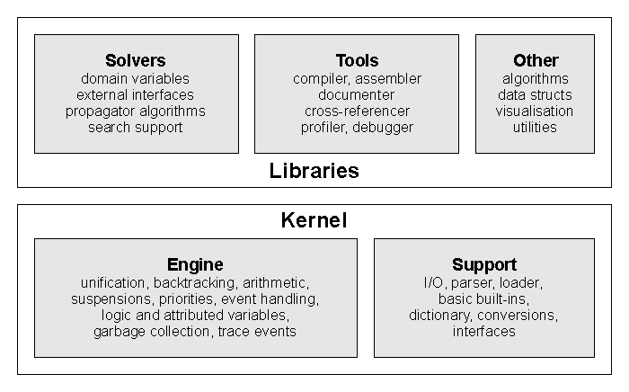
Figure 1: System Structure

Abstract Machine:

ECLⁱPS^e is implemented via an abstract machine: the compiler generates abstract machine instructions, which are then executed by a virtual machine. The abstract machine is a variant of the Warren Abstract Machine (WAM, [Warren (1983)]), with the following main characteristics:

• The engine manipulates pairs of machine words (two 32-bit words, or two 64-bit words), called the value and the tag word. The main purpose of the extra word is to hold type information, but it is used in a few other circumstances as well (garbage collection, variable names, module system authentication, conversion routines). As opposed to single-word implementations, no tag bits are stolen from the value word, meaning that full pointers can be handled, and integers and floats (doubles in the 64-bit case) can be stored with their full machine precision without having to resort to a boxed representation on the global stack. The obvious drawback is usually higher memory consumption.

• Four separate stacks are used, called Global, Trail, Local and Control. As opposed to the original WAM, Local stack (containing environments) and Control stack (containing choice points) are split. This allows immediate choice point space reclamation after a cut or trust instruction, but has no major impact otherwise.

• Dedicated instructions allow the creation of choice points within a clause. These are used for the inline-compilation of disjunctions.

• Unification of compound terms is compiled into two isomorphic instruction streams, corresponding to read mode and write mode [Meier (1990)].

• Environment slot usage is tracked via compiler-generated activity bitmaps. This removes the need for environment slot initialisation, which would otherwise be necessary for precise garbage collection.

Data is always tagged, and the following types/tags are distinguished: four numeric types (integer, rational, float and bounded-real, see section 3.4), with integers having 2 tags/representations (short integer and bignum); atoms (with nil having its own tag); strings (an atomic data type in ECLⁱPS^e); structures (with lists having their own tag); suspensions (section 4.1); handles (section 4.5); plain variables and attributed variables (section 4.2). Further tags are used internally to label various data structures, in particular those that are stored on the global stack, where they are encountered by the garbage collector.

Compiler:

The ECLⁱPS^e compiler was original written in C because compilation speed was considered of major importance. However, for release 6.0, a complete rewrite in the ECLⁱPS^e language itself was undertaken. The main motivation for this higher level approach was that the old compiler had become increasingly difficult to maintain, extend and modify, and that we wanted to incorporate some ideas from Mercury [Somogyi et al. (1995)]. The new compiler is a modular design consisting of

1. The parser (the built-in predicates of the read-family).

2. The source processor (a library used by all tools that process source texts).

3. The actual compiler, translating one predicate at a time (given as a list of clauses) into symbolic abstract machine code.

4. The assembler, turning symbolic abstract machine code into a (relocatable) numeric representation (ECLⁱPS^e object code).

5. The loader, which loads ECLⁱPS^e object code into memory.

Only parser and loader are part of the runtime system, whereas source processor, compiler and assembler are separate libraries. All components communicate via Prolog data structures. Characteristics of the compiler implementation are:

• The compiler is implemented in ECLⁱPS^e itself.

• Input is a term representation of the source, or optionally a representation annotated with source position information, used for generating debugging information in the generated code.

• Each predicate gets normalised into a single-clause form, i.e., the clause structure is converted into disjunctions, and head unifications are made explicit.

• The compiler directly handles clauses with possibly nested disjunctions (forming a directed acyclic control flow graph, similar to [Henderson et al. (1996)]). The retry and trust instructions have variants that are used when the clause already has an environment. This property makes predicate unfolding more effective, by reducing environment allocations and parameter passing.

• Inline disjunctions are indexed. Indexable variables are chosen by analysing the built-in predicates at the beginning of each branch. This is more general than just indexing on head arguments, and guarantees that there is no loss of indexing when a multi-clause predicate is unfolded into an inline disjunction. It also provides a good basis for more elaborate source transformations like unification factoring [Dawson et al. (1996)].

• Indexes are generated individually for every argument/variable for which they might be useful in some possible instantiation pattern, and ordered by selectivity. Selectivity is measured as the ratio between the number of distinct argument values and the number of matching alternatives. During execution, only one index (the most selective one for the actual instantiation pattern) is used. In our experience, this is hardly ever worse, and often much better than simple first-argument indexing, and it does away with the unnatural special status of the first argument. As opposed to full multi-argument indexing, this technique does not lead to code explosion, nor does it require extensive analysis. Mode declarations are taken into account to suppress unnecessary indexes.

• Abstract code postprocessing removes non-reachable code, reduces branching by duplicating short code sequences, eliminates indirect jumps, and generates merged instructions (such as multi-register moves) to speed up execution in an emulated setting.

Garbage Collection:

ECLⁱPS^e has garbage collection for the dictionary and the global/trail stack. The latter is the more important, in particular in the context of constraint processing which tends to be deterministic over long phases. It relies on a mark-and-sweep algorithm inspired by the one developed at SICS [Appleby et al. (1986)]. Because of the double-word architecture of the abstract machine, our collector can employ a faster single-pass marking algorithm, followed by a single-pass compaction sweep. The double-word units make it possible to do all the relocation work on the fly, as described elsewhere [Schimpf (1990)]. Nevertheless, the compaction phase still has to scan all unused memory, therefore an auxiliary copying collector would probably be beneficial when the proportion of garbage is high.

A characteristic of this type of collector is that it relies on the presence of choice points for achieving good incremental behaviour. Long running deterministic programs can, without additional measures, exhibit quadratic growth in collection times and thus arbitrary slowdown. This is due to repeated scanning of the same memory area. One way to overcome this is to manage collections intervals carefully, ensuring a stable ratio between newly allocated memory and the size of the area to be scanned by the collector. An alternative method is the creation of auxiliary choice points (which can serve as markers for memory segment boundaries), but we have abandoned this technique because of its undesirable interference with determinacy assumptions across sequences of abstract machine code.

Finally, it may be worth noting that all trail cleanup is done lazily by the garbage collector, rather than eagerly at the time of choice point removal. Although probably not important in practice, this guarantees that choice point removal is a constant time operation.

2.1 Module System

ECLⁱPS^e’s module system is based on Sepia’s, but was revised in 2000 in the light of previous experience. It was felt that addressing the shortcomings of the module system was critical for our ability to build the multi-solver system architecture we envisaged. The highlights of today’s system are discussed in the following, in particular where they deviate from both the formal [ISO (2000)] or the de-facto Prolog module standard.

Stricter Visibility Control:

Visibility control applies not only to predicates, but to all properties that may be attached to functors, such as goal expansions, read-macros, portray-transformations, structure declarations, and global storage identifiers. Unlike in a name-based module system, the visibility of each functor property can be controlled separately, rather than being linked to the functor’s visibility as a whole. In addition, there are visibility-controlled properties that are not attached to functors, among them a module’s syntax options, character class tables, initialisation and finalisation goals.

Module-sensitive I/O:

Plain Prolog already provides means to modify syntax via operator declarations. In ECLⁱPS^e, there are further configurable syntax options, I/O transformations, and character class tables. Changing such settings will result in disaster unless their scope is clear. They are therefore all subject to module visibility control, and can be local or exported/imported. This is not just a feature of the compiler: it implies that all relevant I/O predicates are sensitive to the module context in which they are invoked. This has proven useful for writing different modules in different language dialects, for defining customised syntax for data formats, and even for reading non-Prolog languages like FlatZinc (the solver input language that goes with the MiniZinc modelling language [Nethercote et al. (2007)]).

Privacy:

Many Prolog module systems do not strictly enforce module privacy, and allow, for instance, local predicates to be invoked from outside the module [Haemmerlé and Fages (2006)]. Our system allows modules to be “locked”, thereby limiting access strictly to their exported interface. This would typically be done for modules that implement critical system functionality. Any such protection mechanism has to preserve Prolog’s meta-programming capabilities. Our design is built around the idea of attaching hidden authentication tokens to module arguments, and requiring these tokens in all built-ins that operate in the space of a locked module.

No static textual interface/implementation separation:

A module’s interface simply consists of the union of all its export directives. No textual separation is required. Instead, tools are provided to extract the interface information from the source or from a loaded module. This interface specification can then be distributed together with the compiled abstract machine code of a module, whenever source distribution is not an option, see figure 7.

Reexport:

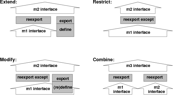
Figure 2: Making modules from modules with reexport

A basic reexport directive is defined in the ISO Prolog module standard [ISO (2000)]. We found that by introducing an additional variant of the form reexport <module> except <items>, we could better support the task of composing modules from existing modules, thus giving the system some flavour of object orientation. Figure 2 illustrates the main concepts: extend the interface of an existing module by adding additional exports; restrict the interface an existing module; modify the interface of an existing module, by reexporting parts of it and redefininig others; combine functionality from existing modules by reeexporting them from a new module.

Lookup Modules, Qualification and Name Conflicts:

In a system with multiple constraint solving libraries, it is highly desirable to use identical predicate names for different computational implementations of the declaratively same constraint. This requires a straightforward handling of name conflicts, which is impossible with the de-facto module standard. Our module system implements a clear separation of the concepts of lookup module and context module, and also allows the qualification of a goal with multiple lookup modules. For example [lazy,eager]:p(X,Y) as a shorthand for lazy:p(X,Y),eager:p(X,Y), invoking two different implementations of p/2. While in plain Prolog it would not make much sense to invoke the (declaratively) same goal twice, with constraint programming it can be beneficial to have several implementations of the (declaratively) same constraint predicate with different operational behaviours, e.g., propagators of different strength and complexity.

No global items:

No Prolog items exist globally, or outside of modules. For instance, built-in predicates receive no special treatment from the module system. They are simply a set of predicates imported from a “language” module. There is also no shared “user” module for implementation hooks.

One consequence of the above features is that it is possible to use a mixture of different programming language dialects within a single user program. Different user program modules can import different language modules. Each language module will typically provide: specific syntax in the form of operators and parsing options; specific semantics in the form of predicates which may add to or replace the standard built-in predicates; and possibly other module-local properties. Several language modules for various Prolog dialects are provided with the ECLⁱPS^edistribution.

Another Prolog system that has invested heavily in the module system design is Ciao [Cabeza and Hermenegildo (2000)]. Ciao’s choices were largely motivated by the requirements of program analysis, but it is reassuring to see that both our groups have arrived at many of the same conclusions: the need for local syntax, stricter and stable interface definitions, correct semantics of module qualification, and the elimination of the special status of built-in predicates.

3 Language Extensions for Modelling and General Programming

When we started work on bringing CLP and Mathematical Programming (MP) together, we realised that our MP collaborators did not necessarily share our view of LP as an ideal framework for expressing constraint models. Being forced to express everything in terms of lists and recursion wasn’t acceptable, given that most MP models are written in terms of arrays and quantification over index ranges. The introduction of loop iterators and arrays was an attempt to address these concerns, but these constructs are useful in general programming as well. The same is true for our structure syntax, which addresses one of Prolog’s long standing software engineering problems. In all these extensions, we have tried to retain the spirit of Prolog by designing them in such a way that they can be easily mapped back into canonical Prolog.

3.1 Arrays

Many attempts to introduce arrays in Prolog (e.g. [Barklund and Bevemyr (1993)]), have considered the problem of destructive updates. This is not what we were after, because we were more interested in declarative modelling than in expressing imperative algorithms that rely on arrays.

Introducing pure logical arrays is not hard, and indeed, Prolog provides them in a way. An array is an ordered collection of items of the same type, with an index set ranging over integers or tuples of integers, and typically constant time access to the items. Since Prolog is dynamically typed, we can use structures as arrays, and regard for instance wd(mo,tu,we,th,fr,sa,su) as an array constant, or create an uninitialised array using functor(DayArray, year, 365). Arguments can be accessed in constant time via arg/3, as in arg(4, WeekdayArray, DayName). It is true that many early Prolog systems imposed limits on the arity of structures, but this has become less of an issue in recent years.

Array Elements in Expressions:

Using arg/3 to access array elements can look clumsy, especially when they are to be used in arithmetic expressions. It would be so much nicer to be able to write Queen[I] =\= Queen[J] instead of

    arg(I,Queen,Qi), arg(J,Queen,Qj), Qi =\= Qj

This is exactly the facility we have introduced. Array syntax is implemented by recognising a new syntactic construct, i.e. variable followed by list (this is backwards compatible with standard Prolog in the sense that the new syntax does not conflict with any previously valid syntax). Technically, we use a trick that is familiar to Prolog implementors: we introduce the new syntax as an alternative syntax for a particular functor. Plain Prolog already does something similar by allowing the square-bracket syntax for the list constructor ./2, or by allowing the ’{}’/1 functor to be written as a pair of surrounding braces. We now simply define a variable immediately followed by a list as syntactic sugar for a structure with the functor subscript/2, with the variable becoming its first, and the list its second argument. For example the input "M[3,4]" is parsed as subscript(M, [3,4]). When a subscript/2 term is printed, the transformation is reversed, unless canonical representation was requested.

The second step is to allow such a term to occur as a function in an arithmetic expression. It is evaluated by adding a result argument and calling the new built-in predicate subscript/3, which is a generalised form of arg/3 and extracts the indicated array element from a possibly multidimensional array. Like all arithmetic evaluation, this is only done in the context of an expression, e.g., the right hand side of is/2, or the arguments of a comparison or other arithmetic constraint. Normal unification is not affected, so M=[](a,b,c), M[2]=b will still fail, analogously to 1+2=3.

Creating Arrays:

To manage multidimensional arrays, represented as nested arrays, a generalisation of functor/3 is useful. We have introduced the predicate dim/2 which can be used in two modes, either to create arrays, or to extract their dimension. For instance:

    ?- dim(M, [2, 3]).
    M = []([](_341, _342, _343), [](_337, _338, _339))

Note that we introduce here the convention of using the [] functor (of arbitrary arity) for arrays. The execution engine may in future exploit this by using a more efficient representation for this particular functor (analogous to optimizations for the list functor ./2). Observe that this choice of functor also implies that empty arrays and empty lists look identical.

3.2 Loops

In the average Prolog program, the vast majority of all recursions represent iterations. Most of them are iterations over lists, some are iterations over structure/array indices, and very few are something else. Our approach to loops has been detailed elsewhere [Schimpf (2002)], so we will only summarise here and point out the usefulness for modelling, especially in connection with arrays.

The ECLⁱPS^e loop construct do/2 can be translated into an auxiliary tail recursive predicate, plus an invocation of this auxiliary. A call

    ?- ( fromto(From,In,Out,To) do Body ).

maps into

    ?- do__1(From, To).
    do__1(Last, Last) :- !.
    do__1(In, Last) :- Body, do__1(Out, Last).

Here, Body is an arbitrary, possibly complex subgoal, From and To are terms shared with the loop’s context, while In and Out are shared with the loop Body. The basic idea is that a simple tail-recursive predicate is generated, where each iteration-specifier (in this example the fromto-term) gives rise to one accumulator (one argument pair). The intuition is that First provides the first accumulator value, Body maps In to Out, providing an accumulator value for the next iteration, eventually terminating when Out=To. Importantly, arbitrarily many fromto-specifiers can be given for a single do-loop, each of them adding one accumulator (which in the general case requires an argument pair) to the recursive predicate.

While the above is enough to express any deterministic iterative recursion, there are of course some very common patterns, like iteration over list elements or integers, for which one can have intuitive abbreviations, see Table 1.

fromto(From,In,Out,To)	general accumulator
foreach(Elem,List)	list iterator and aggregator
foreacharg(Elem,Array)	array iterator
for(I,From,To,[Step])	integer iterator
param(Term)	invariant iterator

Table 1: Some Common Loop Iterators

The do-loop provides the functionalities of iteration, aggregation and mapping, all of which can be combined in a single loop. Iteration specifiers determine what is being iterated over, termination conditions, result accumulation and fixed parameters. In [Schimpf (2002)], we have argued that the proposed loop construct provides better abstraction, better readability, shorter code and improved maintainability compared to the equivalent recursive formulation. At the same time, it can replace many uses of higher order operators (map, foldl) and has advantages in those cases where it applies. When used in the context of problem modelling, it usually has a quite natural declarative reading in terms of quantification over lists or arrays, or index sets.

Loops and Arrays:

Loops and arrays together allow for a rather compact expression of matrix models for constraint problems. Figure 3 shows a model for the N queens problem. Note that, because a loop introduces a local variable scope, we use the param() iterator to indicate values that pass through the iterations unchanged.

    queens_array(N, Board) :-
        dim(Board, [N]),
        Board :: 1..N,
        ( for(I,1,N), param(Board,N) do
            ( for(J,I+1,N), param(Board,I) do
                Board[I] #\= Board[J],
                Board[I] #\= Board[J]+J-I,
                Board[I] #\= Board[J]+I-J
            )
        ).

Figure 3: N queens constraint model with loops and arrays

3.3 Structures

One of the well-known concerns regarding software engineering with Prolog is that using data structures other than lists is problematic. The plain Prolog concept is actually rather elegant: the functionality of structures or tuples is not provided by a separate language construct — instead uninterpreted function symbols assume this role. While this simplicity is conceptually appealing, it turns out to be a real limitation for practical programming, mainly because structure components are identified by position only:

1. The programmer has to remember which positional field has which meaning. References to numeric field positions make the code hard to maintain.

2. Whenever the structure is matched in the code, the arity of the structure has to be known, in addition to the relevant field numbers.

3. If the definition of the structure changes, as fields are added or removed, the programmer needs to update all occurrences of structure templates in the source, and check all field position numbers.

As a consequence, structures are underused in most Prolog programs. The folklore workaround for problem 1 has been to write an access predicate for every structure type, e.g.,

    employee_arg(emp(N,_,_),name,N).
    employee_arg(emp(_,A,_),age,A).

and manipulate the structure exclusively via these access predicates, replacing the generic arg/3. So code like p(emp(N,A,_)) :- ... would have to be written as

    p(Emp) :- employee_arg(Emp,name,N), employee_arg(Emp,age,A), ...

The consistent use of access predicates in lieu of pattern matching is tedious and requires great discipline. It also obscures the code for the compiler: without inter-procedural analysis, a compiler will be unable to do indexing on the argument, since the structure no longer occurs in the clause code. Very likely, the programmer will have to add extra cuts. Moreover, the argument position number might be required in contexts other than just the arg/3 predicate. E.g., in a system that provides a sorting predicate that can sort on a structure argument, one would write sort(2, =<, Emps, EmpsByAge) to sort a list of employee-structures by age. Having such magic numbers in the code is clearly bad practice.

:- local struct(emp(name,age,salary)).     % Translation:
p(emp{age:A,salary:S}) :- ...          =>  p(emp(_,A,S)) :- ...
Emp = emp{salary:Sal}                  =>  Emp = emp(_,_,Sal)
arg(name of emp, Emp, Name)            =>  arg(1, Emp, Name)
sort(age of emp, =<, Emps, EmpsByAge)  =>  sort(2, =<, Emps, EmpsByAge)
update_struct(emp, [salary:NewSal],    =>  Old = emp(A1,A2,_),
                           Old, New)         New = emp(A1,A2,NewSal)

Table 2: Examples of structure syntax and their translation to canonical code

Our solution is simply to provide syntactic sugar in such a way that all the required patterns can be written independently of both the structure’s arity and the order and numbering of the fields. Table 2 shows some examples of this syntax. The obvious first step is to introduce field names, which is done via a declaration like :- local struct(emp(name,age,salary)). This would declare a structure with name “emp” and three fields called “name”, “age” and “salary”. Then we need a better syntax for the situations where the structure as a whole occurs in the code (be it for the purpose of matching against an existing structure or for constructing a new structure). We introduce new syntax, such as emp{age:A,salary:S}, and replace it during parsing by the corresponding structure according to the declaration. The relevant structure fields are referenced by name. Argument positions that are not mentioned give rise to anonymous variables. Importantly, the {}-syntax does not refer to the structure’s arity.

For those circumstances where an argument position number is needed, we reserve the infix operator of/2 and replace terms of the form fieldname of structname by the field number taken from the corresponding struct declaration. The sorting example then becomes sort(age of emp, =<, Emps, EmpsByAge).

As both types of replacement are done at parse time, they apply in whatever context the constructs appear in the program. Note that we do not propose the use of field names at runtime: they are preprocessed away at parse time and nothing is lost in terms of efficiency.

One remaining operation is the change of one or more structure fields, which (in a language without destructive update) amounts to making a new structure in which certain fields are modified while all others remain identical. This would normally require knowledge about all fields and their positions. We introduce a predicate update_struct/4 that encapsulates this knowledge: the last example in Table 2 shows how an instance of this predicate is expanded into the conjunction of two unifications. Again, this is usually a compile-time transformation.

Functional languages usually have syntax like structure.field for accessing a structure field in the context of an expression. In Prolog this is of limited use, because expressions are only evaluated in the context of arithmetic predicates like is/2. We have therefore not introduced a specific notation. However, in an untyped language there is no essential difference between a structure and an array. We can therefore employ our array index syntax, use the field index in its symbolic form, and write, for instance, YearSalary is 12*Emp[salary of emp].

To summarise, the point of our transformations is that the source code no longer contains any mention of either the structure arity or the position numbers of the fields. It is therefore now possible to simply modify the struct-declaration (reordering or adding fields) and recompile, without having to change the rest of the program code. The code also becomes more readable (albeit very slightly longer).

3.4 Numbers

In addition to standard Prolog’s integer and floating point numbers, ECLⁱPS^e supports two further data types: rationals and bounded reals. They are fully integrated into the language, can be mixed with other numeric types in arithmetic expressions, and have their own syntax with corresponding support in parser and term writer. Both types can be viewed as alternatives to floating point numbers.

Rationals:

Rational numbers can be represented accurately and were used in two early ECLⁱPS^e implementations of Gauss/Simplex solvers (by P. Lim and C. Holzbaur [Holzbaur (1995)] respectively). A rational is represented as normalised numerator/denominator pairs of bignums, and written like 1_3. The implementation relies on the GMP library [Free Software Foundation (2009)], which is also used to provide unlimited precision integer arithmetic.

Bounded reals:

A bounded real is a safe approximation of a real number in the form of the closed interval between a pair of floating point bounds, written like 0.99__1.01. Operations on this type use safe interval arithmetic, giving accurate bounds on the results.

The introduction of this number type was a by-product of our work on interval constraint solvers, see section 5.1. Its purpose may become clearer by highlighting the difference between a bounded real number and a variable with an interval domain. Assume a query succeeds in the following way:

    ?- p(X, Y).
    X = _{1.0..2.5}     % an interval domain variable
    Y = 1.9__2.1        % a bounded-real constant
    yes.

This means that variable X remains unconstrained in the interval $[1.0,2.5]$, making every value in this interval a solution. But there is exactly one solution for Y, guaranteed to lie in the interval $[1.9,2.1]$, but not known more precisely. The difference is important in determining whether a computation is finished.

As in Prolog, numbers of the same value but different type (3, 3.0, 3_1 and 3.0__3.0) do not unify in our system. This lack of a canonical representation for integers has caused problems in the interaction with constraint solvers that regard integrality as just another constraint: the order in which constraints are propagated can result in a variable being instantiated to an integer, or to an integral real, and possibly lead to unexpected failures. In hindsight, at least for the purposes of a modelling language, having disjoint number types is probably a mistake, especially since the usual accuracy-based arguments against merging floats and integers apply neither to rationals nor to bounded reals.

4 Kernel Support for Constraints

One aim of ECLⁱPS^e development was to provide an infrastructure for research into constraint solvers. We did not want to build particular domains or solvers into the system kernel, but rather develop them in ECLⁱPS^e and deploy them as libraries. To be able to do so, we needed to identify concepts that are common to classes of solvers, and implement kernel services to provide the necessary infrastructure. The most important of these services are:

• flexible execution control mechanism (delayed goals, suspensions);

• turning logical variables into constrained variables (attributed variables);

• meta-programming language constructs to support these features (suspension handling, matching clauses);

• module and library facilities to support clean packaging and the coexistence of multiple solvers;

• robust support for compile-time preprocessing (macros, inlining, modules);

• abstract interfaces to enable solver-independent components (attribute handlers, generic suspensions, constrained-condition);

• arithmetic support (numeric types, including intervals);

• support for interfacing external solver software (external handles and related trailing functionality).

4.1 Data-driven Execution Control

Coroutining:

One of the early attempts at improving the power of logic programming implementations was the introduction of coroutining: the ability to delay execution of program parts until variables are sufficiently instantiated. With this facility, it is possible to turn inefficient generate-and-test programs into reasonably efficient backtracking search programs, where tests are executed as soon as they can be decided. Such facilities date back at least to Prolog-II [Colmerauer (1982)] and MU-Prolog [Naish (1986)], and were present in ECLⁱPS^e’s predecessor systems in the form of wait declarations (ECRC-Prolog) and delay clauses (Sepia).

Coroutining can be considered the first step towards constraint handling, by virtue of allowing:

• separation of deterministic constraint setup and nondeterministic search code;

• eager constraint-checking behaviour by waiting for sufficient instantiation;

• automatic interleaving of the search process with constraint processing;

• simple forms of propagation, such as delaying until only one variable is left in a goal, and then computing the variable’s value.

Suspensions:

To support constraint propagation more generically, we decided to reuse the delay/wake machinery for coroutining that we had inherited from Sepia, but to allow additional trigger conditions for waking. Since such conditions are solver-specific, and solvers were meant to be definable in libraries, we decided to separate the shared concept of a “delayed goal” from the different waking conditions. The abstract machine data type we introduced to represent a delayed goal without waking conditions is called a suspension.

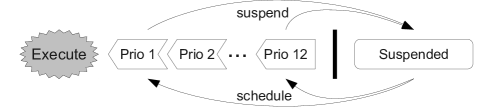
Figure 4: Structure of the resolvent

Figure 4 shows the structure of the resolvent, i.e., the collection of goals still to be satisfied. It consists of an active part (ordered by priorities, see below) and the currently inactive, suspended part. Goals in the suspended part of the resolvent are represented by suspensions. A goal enters the suspended part of the resolvent when it is created via the make_suspension/3 built-in, analogously to the way a goal becomes a part of the active resolvent when created via call/1.

We draw attention to the fact that our system maintains an explicit representation of the suspended resolvent. If a suspended goal were just a data structure stored within an attribute, then it would be entirely the programmer’s responsibility to enforce the goal’s semantics, i.e., to invoke it eventually. If the goal were never invoked, it would be incorrectly considered true. In our scheme, the abstract machine keeps track of each delayed goal right from the moment it is created, independently of its attachment to variables or trigger conditions. Cases of unsolved subgoals (“floundering”) are therefore always detectable. Further advantages are that suspensions can be manipulated via generic kernel primitives, and that they can be displayed in a solver-independent fashion by the toplevel and the debugger’s delayed goal viewer.

Priorities:

In a constraint solving system, a single event (such as updating a domain bound) will typically wake many constraint agents (represented by suspensions) at once. It is helpful to have some control over the order in which they are actually executed, since they may exhibit vastly different performance characteristics: constraints with few variables will generally propagate faster, linear-time propagators faster than quadratic ones, etc. We therefore associate suspensions with priorities, which determine the execution order after waking. A simple system with 12 priority levels is used. Goals that wake up with higher priority can interrupt currently running goals with lower priority. High-priority goals can also be used for tracing and debugging, and for creating data-driven animated visualisations. Although the scheme imposes some overhead, we have found the functionality worthwhile. Recently, other Constraint Programming systems have also implemented priorities [Schulte et al. (2009)].

Waking Conditions:

The usual (though not the only) way to provide for waking of suspensions is to associate them with conditions that occur within a specified set of variables. Three of these conditions are pre-defined by the ECLⁱPS^e kernel:

Instantiation

is the most obvious one: with this condition, a delayed goal gets woken when at least one of the variables in a specified set becomes instantiated.

Binding

subsumes instantiation, but also includes aliasing of variables. It is required in a case like the sound difference predicate X ~= Y, in other systems known as dif(X,Y). As written, such a goal will delay because it is not decidable. But unifying of X with Y should wake it and lead to failure, even without instantiation. When suspended under the binding condition, a goal will wake when any two variables in the specified set are unified, i.e., whenever the number of variables in the set is reduced. Thus, dif/2 can be written as

dif(X,Y) :- (X==Y -> fail ; suspend(dif(X,Y), 3, [X,Y]->bound)).

Here, the suspend/3 built-in creates a suspension of priority 3 for dif(X,Y), and associates as waking condition any binding within the variable set $\{X,Y\}$.

Constraining

is unique to ECLⁱPS^e and is an abstract condition indicating that a variable was constrained in some way. The concrete meaning is defined by the libraries that implement the constrained variables. The abstract condition makes it possible to write generic, solver- and domain-independent tools, such as the following predicate that eagerly prints a message whenever a variable becomes further constrained during computation:

report(X) :-
    write(constrained(X)), suspend(report(X), 1, X->constrained)).

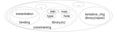
Figure 5: Hierarchy of the three generic and some library-defined waking conditions

Other waking conditions can be defined by libraries, using generic built-ins for manipulating suspension lists and attributed variables (section 4.2). Figure 5 shows the hierarchy of generic conditions together with examples of library-defined ones: the interval solver library(ic) defines 4 waking conditions: lower and upper domain bound change, creation of a hole in the domain, and type restriction from real to integer. All these conditions constrain the variable further and are thus subsumed by the constrained condition. The repair library on the other hand implements a waking condition called tentative_change, which is not considered as constraining the variable. Finally, it is possible to have waking conditions that are not related to variables, but instead to certain points in execution. One such example is the success of the subgoal in an all-solutions predicates like findall/3, where we want to make sure that no goals are left delayed.

Suspension States and Demons:

During execution, a suspension data structure may be attached to multiple waking conditions (typically related to variables). Since we have a two-stage waking process of (1) scheduling for priority-based execution, and (2) actual execution from the front of the priority-queue, we need to take care of multiple redundant waking. This is implemented by having stateful suspensions indicating whether they are in the suspended, scheduled, or already executed state.

Another original enhancement of the suspension system that was introduced for the needs of constraint propagation was the concept of demons: while a goal that simply waits for the instantiation of one variable will only be suspended once and woken once, a goal that performs a task like domain bound propagation may be woken many times, each time re-suspending as exactly the same goal with the same variables. To better support this requirement, we introduced predicates that remain in the suspended resolvent even after having been woken. Declaratively, this can be viewed as these predicates have an implicit (and thus efficient) self-recursive call.

4.2 Implementing Constrained Variables

ECLⁱPS^e’s predecessor system Sepia had delay-variables, to which delayed goals were attached by the system in an opaque way. This was replaced by an open and more flexible mechanism, namely attributed variables [Holzbaur (1992)], which are a generic way to attach (meta) information to a logical variable. Examples of such information are:

• lists of goals to be woken on certain variable-related events (suspension lists);

• unary constraints on the variable, like type or domain;

• link to the representation of the variable in an external solver;

• information with no effect on semantics, like debugging information or variable name.

We typically use coarse-grained attributes: a module (often a constraint solver) defines no more than one attribute, but the attribute itself will normally be a compound data structure.

Since attributes are usually meant to modify the semantics of the variables they are attached to, they affect a range of generic operations in the basic Prolog system, unification being only the most obvious one. We believe that ECLⁱPS^e is unique in the degree to which it extends basic Prolog semantics to attributed variables. As soon as an attribute definition is loaded into the system, it optionally installs handlers and hooks, which the generic system operations can use on encountering a variable with the new attribute. The operations whose semantics can be extended in this way are listed below.

Unification:

An attribute handler is invoked immediately after an attributed variable has been unified with a nonvariable or another attributed variable. The handler must first check whether the unification is allowed (by considering, for example, the domain information within the attribute). If so, goals associated with the variable have to be woken if their respective waking conditions apply. In case of variable-variable unification, a new attribute for the resulting variable may have to be computed.

Unifiability and subsumption testing:

Specialised handlers can be provided to compare domains and thus extend the system’s generic operations for unifiability testing (not_unify/2) and subsumption testing (variant/2 and instance/2).

Term copying:

This handler enables the copy_term/2 built-in to give a meaningful result for attributed variables. Typically, any unary constraint (such as the domain) on the variable would be reflected in the copy.

Anti-unification:

This is an interface supporting Generalised Propagation (section 5.3) [Le Provost and Wallace (1993)] by defining its fundamental operation: anti-unification computes the most specific generalisation of two terms, as precisely as the expressiveness of a particular attribute allows. For example, given the availability of finite-domain attributes, two integers can be generalised into a variable whose domain ranges over these two integers.

Constraining:

We discussed above the generic constrained waking condition. In order to define what it means for a particular type of attributed variable to become “more constrained”, all code that implements operations on the corresponding attribute must notify the system accordingly. For instance, the interval constraint solver can constrain variables by excluding domain values in various ways, and should therefore notify the system on these occasions.

Bounds access:

The system defines the built-in predicates set_var_bounds/3 and get_var_bounds/3 to provide a generic way to access numeric variable bounds. The built-ins obtain their information via a handler predicate defined together with the attribute. This can be used for solver communication, e.g., querying the propagation results of other solvers, or broadcasting new bounds to others.

Attribute-specific waking conditions:

New waking conditions are made available simply by allocating a slot for a corresponding suspension list within an attribute. To delay a goal under the new condition, the system simply inserts a suspension into this list. An interval variable, for instance, has one suspension list associated with changes to the lower bound, and one for upper bound changes. These lists are in addition to the pre-defined lists for instantiation, aliasing and general constraining (figure 5). The primitive solver operations for changing variable bounds are responsible for scheduling the goals from the appropriate list(s): a lower bound change, for instance, should schedule the lower bound list as well as the constrained-list. Once a suspension list is scheduled for execution, its member goals will start executing according to their priorities, see section 4.1.

4.3 Preprocessing, or Getting term-expansion Right

Most Prolog systems implement the term-expansion facility. This is a powerful way of rewriting terms during compilation, and has many useful applications. However, its design is too simplistic in several respects. There are at least three contexts in which one may want to transform an input term: (1) when it occurs as a clause during compilation, (2) when it occurs as a goal during compilation, and (3) when it occurs during general I/O (when it is a data structure that needs to be translated to/from some internal representation). The traditional term-expansion mechanism makes it hard to distinguish (1) and (2), and is not able to do (3) because it is only applied during compilation, not term-reading in general. Other shortcomings are the lack of cooperation with the module system and the problem of safely combining different expansions: term_expansion clauses are global, and committed to the first one that succeeds. The clauses themselves have no knowledge about the module context in which they occur, and thus cannot be selective in their transformations. Some implementations have added goal expansions to partly address these problems.

We have opted for a different, more disciplined mechanism: transformations are always associated with functors, and their visibility is controlled by the module system. Moreover, there are three types of input transformations according to the three categories mentioned above, plus corresponding output transformations. The different types are described below. Because the transformations are independent of each other, a single functor can have more than one associated transformation.

Clause expansion:

An example is the declaration for grammar rules:

:- export macro((-->)/2, trans_grammar/3, [clause]).

It says that whenever a clause with toplevel functor (-->)/2 is encountered during compilation, in a module where this transformation has been imported, it must be transformed by the transformation predicate trans_grammar/3. The latter takes as arguments the original clause plus its context module, and returns a transformed clause. Apart from being applied more selectively, this is similar to term-expansion.

Goal expansion:

Goal expansions are declared like

:- inline(p/1, trans_p/3).

meaning that occurrences of p/1 goals will be expanded using the transformation predicate trans_p/3. This takes as arguments the original goal and its context module, and returns a transformed goal. Unlike in the other cases, there is no visibility specification for this expansion: its visibility is linked to the visibility of the p/1 predicate, i.e., the transformation will be applied in all modules where p/1 is visible, or even when qualified calls to p/1 are made (e.g. m:p(X)). This ensures that goal transformations always match the corresponding predicate definitions, which is of special importance in the case where different definitions and different goal expansion rules for the same predicate name co-exist in different libraries. Goal expansions are used widely in ECLⁱPS^e, e.g., for implementing is/2, for compile-time preprocessing of constraints, and for the do-loop transformation (section 3.2).

General input macro:

A general term macro declaration looks like

:- local macro(foo/1, trans_foo/2, [term]).

It means that every time a foo/1 term is read (even as a sub-term) in a module context where this declaration is visible, it is transformed by the predicate trans_foo/2. This transformation is done by the parser, not only in the context of the compiler, but whenever a predicate of the read/1 family is invoked from within the right module context. This type of transformation is used internally to implement structure syntax (section 3.3). Transformations are done in a bottom-up fashion, so any arguments of foo/1 are already transformed when trans_foo/2 receives the term for processing. Macros can be declared local or exported.

Output transformations:

The symmetric counterparts of the three input transformations above are output transformations: they are of type clause, goal or term, and are also associated with a functor:

:- local portray(foo/1, trans_foo/2, <type>).

These allow an internal representation to be turned back into an external representation before output. Because this a term-to-term mapping, it can be performed before arbitrary term output predicates. This is more flexible than the traditional portray/1 hook, which produces output directly (and has rightly been omitted from the ISO standard, but without having been replaced by a better alternative).

4.4 Destructive Updates and Timestamps

The usefulness of attributed variables would be quite limited without destructive updates. Even if destructive updates were unavailable on the language level, they would be needed for implementation-level data structures. Obvious examples are updating a variable’s domain, or modifying a suspension list, both stored inside an attribute. On the abstract machine level, these all amount to replacing one non-variable value with another — an operation that does not occur in pure Prolog. To allow this in the presence of backtracking, we have to extend the trailing mechanism, such that it allows resetting the content of a location to an arbitrary previous value. This change, however, creates the new problem of multiple redundant trailing of the same location: a location can be modified arbitrarily many times, but only the value that was current when the previous choicepoint was created must be restored. The first published solution [Aggoun and Beldiceanu (1990)] to this problem involves keeping choicepoint-related timestamps together with the trailed locations. These timestamps indicate whether a location has already been trailed since the last choicepoint was created. In ECLⁱPS^e we use two related techniques: if we have control over the layout of the trailed data structure, we add a timestamp field to it. As the timestamp, we use the global stack pointer at the time of the last choicepoint creation. To force this to be unique, we make sure that at least one global stack cell is allocated along with every choicepoint. In case we cannot add a timestamp to the data (e.g. in the setarg/3 predicate which destructively updates an argument of an arbitrary Prolog structure), we use the address of the old value as an indication of its age, and trail only if it is older than the last choicepoint. The new value is forced to have an address that represents the age of the binding, if necessary by allocating an auxiliary global stack cell and adding an indirection. The technique is similar to a class of techniques proposed by Noyé [Noyé (1994)].

4.5 Interfacing External Solvers

We have successfully connected external solver libraries to ECLⁱPS^e, such as the mathematical programming system COIN-OR [Lougee-Heimer (2003)] and the constraint library Gecode [Schulte et al. (2009)]. To be efficient enough, these interfaces must be low-level. They are typically written in C/C++, use dynamically linked libraries, and require direct access to solver data structures on one hand, and ECLⁱPS^e’s abstract machine data structures on the other. They are supported by the following kernel features.

Low Level Programming Interface:

This interface allows direct access to the abstract machine’s data representation. Apart from interfacing external solvers, it is also used for connecting other software, such as databases, or to implement procedural algorithms more efficiently than would be possible in Prolog.

The interface exposes a subset of the operations used to implement the ECLⁱPS^e runtime system itself, and consists of macros, type definitions and interface functions. It is powerful and efficient, but requires detailed knowledge about the internal architecture and concepts. A low-level interface exists for the C programming language and, with wrapper classes, for C++. It is bi-directional in that it enables the implementation of external predicates in C/C++, but also allows ECLⁱPS^e goals to be constructed and executed from C/C++.

External Data Handles:

Recurring problems in interfacing general software to a Prolog-like system are the handling of backtracking and garbage collection. While Prolog data structures are discarded from the stacks on backtracking, or removed by the garbage collector when they are no longer accessible, the same has to be arranged explicitly for data allocated by interfaced software. We achieve this by having a special Prolog-side data type (called a handle) which refers to the external data. In addition, every handle is associated with a method table which lists methods specific to the data that is being pointed to, among them a method for releasing the storage. When the handle is discarded, the external object is automatically freed.

Handles cannot be simple tagged pointers directly to external data, because the Prolog abstract machine will blindly make copies of such tagged pointers, making it difficult to keep track of whether the data is still referenced. Our solution is to introduce an indirection: the external data is referenced only once from a dedicated global stack cell (called an anchor), which in turn can have arbitrary references from other Prolog objects (Figure 6). When the garbage collector detects that the global stack anchor has become garbage, it invokes the external object’s free-method. The object must also be freed when the anchor is popped on backtracking — we achieve that with a special trail entry that, on backtracking, leads to invocation of the free-method. Should the anchor become garbage before backtracking, the trail entry becomes redundant and is removed by the garbage collector together with the anchor itself.

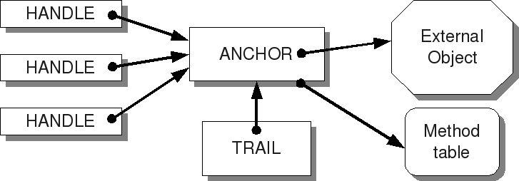
Figure 6: External Data Handles

Apart from deallocation, we also need to consider the case where the external object gets modified in the course of the computation. If the Prolog side backtracks to a state before the external modification was made, the modification will typically have to be undone. We do this by trailing pointers to user-defined C/C++ “undo-functions”, which will then be invoked on backtracking. As with the trailing of destructive updates, the technique has to be combined with a timestamping mechanism to be scalable.

5 Library Examples

For the constraint application programmer, working with ECLⁱPS^e involves: problem modelling using an extended Prolog; choosing solver libraries appropriate for particular problem domains; considering libraries for generic techniques, or for specific solver hybridisation methods; implementing search heuristics, solver cooperation, or problem-specific propagation by using ECLⁱPS^e as a programming language. This section presents some typical libraries that the system provides as building blocks to support these tasks.

5.1 A “Native” Solver: Interval Constraints

The interval solver library(ic) provides unified handling of continuous and integer domains. Its conceptual computation domain is the real numbers, plus infinities. Numbers can be constrained to be integral, and constraints can range over a mixture of integral and non-integral variables. A wide range of constraints is supported, including linear and nonlinear arithmetic operations, and a number of symbolic constraints such as alldifferent/1. The functionality subsumes that of a finite domain solver. The code in figure 3 uses this library.

The solver is implemented natively, with much of the code written at the ECLⁱPS^e language level. Interval variables are implemented as attributed variables, and their bounds are represented as a pair of floating point numbers. The kernel’s interval arithmetic is used, keeping rounding errors under control. Integer variables can have additional bitmaps to represent holes in their domain, and bitmap operations are accelerated using functions interfaced through the low-level C interface.

Most of the constraints are implemented using AC-3 style propagators [Mackworth (1977)], which recompute domains after changes. The propagators themselves are simply delayed goals with suitable waking conditions. The solver defines new waking conditions appropriate for its domain variables: min (lower bound change), max (upper bound change), hole (non-bound domain reduction), and type (imposition of integrality). As the general mechanism of attributes and suspensions is used for implementing constraint behaviour, there is no need for additional low-level support. The following illustrates how to implement geq(X,Y), a simple $X\geq Y$ constraint, where X and Y are variables or integers:

   geq(X, Y) :-
       ic:get_max(X, XH), ic:get_min(Y, YL),
       ic:impose_min(X, YL), ic:impose_max(Y, XH),
       ( var(X),var(Y) -> suspend(ge(X,Y), 0, [X->ic:max,Y->ic:min])
       ; true ).

We use a suspension that wakes when either the upper bound of X or the lower bound of Y is narrowed. Any change in bound is propagated to the other variable using library primitives: the value for the bound that may have changed is obtained by get_max/get_min, then that bound is imposed on the other variable using impose_min/impose_max. The interested reader is referred to the documentation provided with ECLⁱPS^e for more details.

As no hidden mechanism is used, and assuming the solver exports a small number of fundamental primitives, such as access to domain bounds, a user can implement additional constraints on the ECLⁱPS^e level. This is particularly interesting given the large number of potentially useful “global” constraints [Beldiceanu et al. (2005)], and we have been fortunate enough to receive external contributions of such constraints, packaged as ECLⁱPS^e libraries for distribution.

The interval solver also makes extensive use of the preprocessing facilities (goal expansion, section 4.3) for compile-time transformations of constraints. For example, we normalise arithmetic expressions and expand the constraint X#>=5*(X+Y)+2 into its internal form ic:ic_lin_con(6, 1, [2*1, 5*Y, 4*X]). When printed, the internal form is translated back into readable form via an output transformation.

5.2 An External Solver Interface: Eplex

The motivation for interfacing to an external solver comes from the wish to take advantage of existing software: comparisons have shown that a state-of-the-art Mathematical Programming (MP) solver can be 1-3 orders of magnitude faster than one purpose-written for CLP systems [Shen and Schimpf (2005)]. Such external solvers typically provide an API in a popular imperative language such as C/C++.

ECLⁱPS^e’s library(eplex) [Shen and Schimpf (2005)] is a common interface to several state-of-the-art MP solvers, such as CPLEX (www.ibm.com), Xpress-MP (www.fico.com) and COIN-OR [Lougee-Heimer (2003)]. It allows the optimisation of linear constraints over continuous and integer variables by an external solver. The simplest mode of use consists in modelling a problem in ECLⁱPS^e, passing it to the external solver, and returning the results. But more importantly, the interface allows a tight integration of the external solver’s operation with the Prolog side’s data-driven propagation and backtracking-based search framework. Each MP problem can then be regarded as being represented by a single compound constraint, and problem solving can be triggered in a data-driven way. A problem can be repeatedly modified (by adding more constraints to it, and/or updating the variable bounds) and re-solved, with backtracking returning a problem to its previously state.

The eplex library is written in both ECLⁱPS^e and C, using the low-level interface described in section 4.5. Attributed variables and suspensions are used to provide the constraint-like data-driven behaviour: a demon suspension which invokes the MP solver is created, and woken whenever the specified triggering conditions are met. The MP solver is represented by an external data handle, and each ECLⁱPS^e variable involved in an MP problem is linked to the solver through its attribute. The interface is fully dynamic: any change made to a problem after setup (e.g. adding constraints, changing variable bounds), is reflected in the external solver. To maintain the logical behaviour of the whole system, any such changes are undone on backtracking. Implementation-wise, this relies heavily on our trailing and timestamping facilities (sections 4.5 and 4.4).

5.3 A Higher-Level Technique: Generalised Propagation

The Generalised Propagation solver library(propia) [Le Provost and Wallace (1993)] interprets program annotations and extracts deterministic information from arbitrary disjunctive sub-problems. It is very useful for prototyping unusual and problem-specific constraints, that would otherwise need extensive reformulation into standard constraints. It is an example of a library that relies purely on the generic system interface to attributed variables (the concepts of constrainedness and generalisation), and can therefore cooperate with any domain-oriented solver.

5.4 An Orthogonal Paradigm: Repair-Based Search

The repair and tentative libraries implement techniques that differ radically from the framework of domain solvers, being rather closer to Local Search techniques: tentative values are attached to variables, and the amount of constraint violation is measured. By varying the tentative values, a local search procedure can reduce constraint violations, and find better solutions [Van Hentenryck and Michel (2005)]. There are many ways of combining this with constraint propagation and tree search, one successful example being unimodular probing [El Sakkout and Wallace (2000)]. Interestingly, we were able to implement this paradigm using the same underlying techniques as the other solvers. We use attributes to attach tentative values to variables, and we are able to use attribute handlers and suspended demons to update violation counts, conflict sets, and tentative invariants in an incremental fashion. The common architecture facilitates the implementation of hybrid schemes that combine propagation with Local Search.

6 Programming Larger Applications

ECLⁱPS^e has been used to implement a number of large applications, many involving constraint solving. Such applications are characterised by:

Size:

Typically moderately large amounts of ECLⁱPS^e code, some of it concerned with actual problem modelling, but much of it performing general data processing tasks: hundreds of predicates, dozens of modules, tens of thousands of lines of code. Although this does not reach the dimensions of very large industrial software (partly due to the greater compactness of Prolog code), it goes beyond what is common in academic use, and highlights plain Prolog’s limitations with respect to larger scale software engineering.

Interfacing requirements:

Interfacing with a software environment, e.g., retrieving data from a database, producing results in the form of web pages, interacting via graphical user interfaces. Frequently, such requirements also come in rather arbitrary form, such as “must be a Java application”.

Quality requirements:

Code must be designed, written, tested, documented and maintained to certain standards.

These issues are in part addressed by the language extensions we have discussed earlier, such as the module system (section 2.1) and data structure declarations (section 3.3). Our approach to addressing the host software interfacing requirements involves a high-level, language-independent communication scheme that has been described elsewhere in detail [Shen et al. (2002)]. The main ways to achieve code quality are through training, methodology and tools, which we review in the following.

Methodology:

Solving large-scale combinatorial optmisation problems presents additional challenges, as compared to standard software development. ESPRIT project 22165 (CHIC-2), in which ECLⁱPS^e served as a platform, produced a high-level methodology [Gervet (2001)]. Concrete technical development guidelines were formulated by Simonis [Simonis (2003)]. These build on more basic training and tutorial material, such as [Cheadle et al. (2003), Apt and Wallace (2007), Simonis (2010)].

Development Environment:

Apart from supporting the build process and interactive execution, the development environment provides tools that give information about the state of an executing program. The main ones are the tracer and the data inspector.

The tracer combines the classical port-oriented box model [Byrd (1980)] (enhanced with goal stack display and filtering capabilities) with source-oriented viewing and breakpointing facilities. The tracer’s architecture is layered: during program execution, low-level trace events are generated by the abstract machine emulator and combined with debug information that the compiler has inserted into the code. A second layer maps the low-level events into box-model events and reconstructs a full call stack. A third layer presents this information via a user interface.

Whenever execution is halted, the current state can be inspected through a tree-browser that allows to traverse and display all data structures associated with the current goal or its ancestors. This tool has proven indispensable when dealing with complex nested data structures in large programs. With coroutining and constraints, an additional important tool is the delayed goals viewer, which displays the suspensions and their state.

The debugging tools have a choice of user interfaces: a traditional command-line interface, as well as GUIs in Tcl/Tk and in Java. The tools are independent from the rest of the development environment, and can be attached any running (even embedded) ECLⁱPS^e engine via a stream-based protocol.

Structured Documentation:

We support structured comment/2 directives as a way to formally add documentation to source code. These directives can relate to a whole module, to predicates or to data structures. For instance, for predicates the comment directive contains fields like: a detailed description, mode information, summary, arguments, example usages, etc. Although devised independently, our solution is similar to the LPdoc system of Ciao Prolog [Hermenegildo (2000)] in that the documentation is provided in the form of directives. One difference is that we do not define our own mark-up language for formatting text, but rely on common HTML format.

Comment directives are processed in two steps: first they are extracted from the source file by the icompile tool, together with other directives that describe the module’s exported interface. The information is put into an ECLⁱPS^e interface information (eci) file. The rationale for this is that this file can be distributed together with a precompiled (eco) file in place of the module source code (Figure 7).

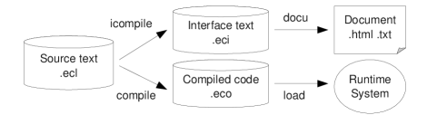
Figure 7: Source Processing

In a second step, the document library tools process the information in the eci file to produce reference documentation for modules, for example in the form of HTML pages with indexes and cross-links.

Unit Testing and Code Coverage:

The test_util library provides support for unit testing. It allows to write simple rules relating a goal with an expected outcome. This library was initially developed to support the daily automatic test and build of ECLⁱPS^e itself, but has since been used to test application programs as well. It is supplemented by a code coverage tool that displays how frequently each code point was executed during testing. In this way, full test coverage can be ensured.

Profilers and Instrumentation:

For performance tuning, we have developed a number of tools: a timing profiler based on sampling the abstract machine’s program counter, which works with fully optimised code and displays a flat profile of the predicates in which time was spent. Another profiler is built on top of the infrastructure for the box model tracer; it creates a profile in terms of transitions through box model ports, and needs the code to be compiled in debug mode. An even more general library provides code instrumentation by source expansion, and can be used for analysing specific resource usage, in particular memory.

7 Conclusion

In the long history of ECLⁱPS^e, many good ideas were incorporated, but quite a few bad decisions were taken as well. Many of them were revised later, although this might not be surprising given the lifespan of the system. The usual lessons regarding software engineering apply, in particular those about defining clean interfaces and allowing for components to need replacement over time.

Only few of the commercial applications developed with ECLⁱPS^e have been documented in accessible publications. However, open-sourcing has enabled the user community to contribute. The contributions so far have been of high quality and, as expected, largely in the form of libraries. We hope very much that this trend will continue.

There are many projects for the future which cannot be listed here — a large system like ECLⁱPS^e always has construction sites. A quite substantial but worthwhile job would be to revive the parallel version of the system, which was mothballed almost 15 years ago. On the language level, we want to make the system easier to use for constraint problem solvers who don’t want to know about the intricacies of Prolog. We also plan to continue our successful strategy of interfacing third party solver software, and to strengthen ECLⁱPS^e’s role as a glue system.

We hope that our past work has been original and influential in the wider Prolog community. We also hope that we have played some role in demonstrating the benefits of Logic Programming to a wider audience in the world of optimization and decision support.

References

- Aggoun and Beldiceanu (1990) Aggoun, A. and Beldiceanu, N. 1990. Time stamps techniques for the trailed data in constraint logic programming systems. In SPLT’90, 8 Séminaire Programmation en Logique, 16-18 mai 1990, Trégastel, France, S. Bourgault and M. Dincbas, Eds. 487–510.
- Appleby et al. (1986) Appleby, K., Carlsson, M., Haridi, S., and Sahlin, D. 1986. Garbage collection for Prolog based on WAM. Tech. Rep. R86009B, Swedish Institute of Computer Science.
- Apt and Wallace (2007) Apt, K. R. and Wallace, M. 2007. Constraint Logic Programming using ECLiPSe. Cambridge University Press, Cambridge, UK.
- Barklund and Bevemyr (1993) Barklund, J. and Bevemyr, J. 1993. Prolog with arrays and bounded quantifications. In LPAR ’93: Proceedings of the 4th International Conference on Logic Programming and Automated Reasoning. Springer, 28–39.
- Beldiceanu et al. (2005) Beldiceanu, N., Carlsson, M., and Rampon, J.-X. 2005. Global constraint catalog. Technical Report T2005-06, Swedish Institute of Computer Science, Kista.
- Bocca (1991) Bocca, J. 1991. MegaLog – A Platform for Developing Knowledge Base Management Systems. In Proc. Second Int. Symposium on Database Systems for Advanced Applications (DASFAA ’91), Tokyo.
- Byrd (1980) Byrd, L. 1980. Understanding the Control Flow of Prolog Programs. In Logic Programming Workshop. Debrecen, Hungary.
- Cabeza and Hermenegildo (2000) Cabeza, D. and Hermenegildo, M. 2000. A new module system for Prolog. See Lloyd (2000), 131–148.
- Cheadle et al. (2003) Cheadle, A. M., Harvey, W., Sadler, A. J., Schimpf, J., Shen, K., and Wallace, M. G. 2003. ECLiPSe: A tutorial introduction. Tech. Rep. 03-1, IC-Parc, Imperial College London.
- Colmerauer (1982) Colmerauer, A. 1982. PROLOG II Manuel de Référence et Modèle Théorique. Tech. Rep. ERA CNRS 363, Groupe Intelligence Artificielle, Faculté des Sciences de Luminy.
- Dawson et al. (1996) Dawson, S., Ramakrishnan, C. R., Skiena, S., and Swift, T. 1996. Principles and practice of unification factoring. ACM Trans. Program. Lang. Syst. 18, 5, 528–563.
- Dincbas et al. (1988) Dincbas, M., Van Hentenryck, P., Simonis, H., Aggoun, A., Graf, T., and Berthier, F. 1988. The constraint logic programming language CHIP. In International Conference on Fifth Generation Computer Systems 1988. Tokyo.
- Dorochevsky et al. (1992) Dorochevsky, M., Li, L.-L., Reeve, M., Schuerman, K., and Véron, A. 1992. ElipSys: A parallel programming system based on logic. In Logic Programming and Automated Reasoning. Lecture Notes in Computer Science, vol. 624. Springer, 469–471.
- El Sakkout and Wallace (2000) El Sakkout, H. and Wallace, M. G. 2000. Probe backtrack search for minimal perturbation in dynamic scheduling. Constraints 5, 4, 359–388.
- Free Software Foundation (2009) Free Software Foundation 2009. The GNU Multiple Precision Arithmetic Library. Free Software Foundation. http://gmplib.org.
- Frühwirth (1998) Frühwirth, T. 1998. Theory and practice of Constraint Handling Rules. Logic Programming 37, 1-3, 95–138.
- Gervet (1997) Gervet, C. 1997. Interval propagation to reason about sets: Definition and implementation of a practical language. Constraints 1, 3, 191–244.
- Gervet (2001) Gervet, C. 2001. Large scale combinatorial optimization: A methodological viewpoint. In Series in Discrete Mathematics and Theoretical Computer Science. DIMACS, 151–175.
- Haemmerlé and Fages (2006) Haemmerlé, R. and Fages, F. 2006. Modules for prolog revisited. In ICLP, S. Etalle and M. Truszczynski, Eds. Lecture Notes in Computer Science, vol. 4079. Springer, 41–55.
- Henderson et al. (1996) Henderson, F., Somogyi, Z., and Conway, T. 1996. Determinism analysis in the mercury compiler. Australian Computer Science Communications 18, 337–346.
- Hermenegildo (2000) Hermenegildo, M. V. 2000. A documentation generator for (C)LP systems. See Lloyd (2000), 1345–1361.
- Holzbaur (1992) Holzbaur, C. 1992. Metastructures versus attributed variables in the context of extensible unification. In PLILP, M. Bruynooghe and M. Wirsing, Eds. Lecture Notes in Computer Science, vol. 631. Springer, 260–268.
- Holzbaur (1995) Holzbaur, C. 1995. OFAI clp(Q,R) manual. Tech. Rep. TR-95-09, Austrian Research Institute for Artificial Intelligence, Vienna.
- ISO (2000) ISO. 2000. ISO/IEC 13211-2:2000: Information technology – Programming languages – Prolog – Part 2: Modules. International Organization for Standardization, Geneva.
- Le Provost and Wallace (1992) Le Provost, T. and Wallace, M. 1992. Domain-independent propagation (or Generalised Propagation). In Proceedings of the International Conference on Fifth Generation Computer Systems (FGCS’92). 1004–1011.
- Le Provost and Wallace (1993) Le Provost, T. and Wallace, M. 1993. Generalized constraint propagation over the CLP Scheme. Journal of Logic Programming 16, 3-4 (July), 319–359. Special Issue on Constraint Logic Programming.
- Lloyd (2000) Lloyd, J. W., Ed. 2000. Computational Logic - CL 2000, First International Conference, London, UK, 24-28 July, 2000, Proceedings. LNCS, vol. 1861. Springer.
- Lougee-Heimer (2003) Lougee-Heimer, R. 2003. The Common Optimization INterface for Operations Research: Promoting open-source software in the operations research community. IBM Journal of Research and Development 47, 1, 57–66. http://www.coin-or.org.
- Mackworth (1977) Mackworth, A. K. 1977. Consistency in networks of relations. Artificial Intelligence 8, 99–118.
- Mariott and Stuckey (1998) Mariott, K. and Stuckey, P. 1998. Programming with Constraints: an Introduction. MIT Press, Cambridge, MA.
- Meier (1990) Meier, M. 1990. Compilation of compound terms in Prolog. In Proceedings of the North American Conference on Logic Programming 1990. Austin.
- Meier et al. (1989) Meier, M., Aggoun, A., Chan, D., Dufresne, P., Enders, R., de Villeneuve, D. H., Herold, A., Kay, P., Perez, B., van Rossum, E., and Schimpf, J. 1989. SEPIA - an extendible Prolog system. In Proceedings of the 11th World Computer Congress IFIP’89. San Francisco, 1127–1132.
- Naish (1986) Naish, L. 1986. Negation and control in Prolog. Number 238 in Lecture Notes in Computer Science. Springer-Verlag, New York.
- Nethercote et al. (2007) Nethercote, N., Stuckey, P. J., Becket, R., Brand, S., Duck, G. J., and Tack, G. 2007. MiniZinc: Towards a standard CP modelling language. In Principles and Practice of Constraint Programming, Proc., C. Bessiere, Ed. LNCS, vol. 4741. Springer, 529–543.
- Noyé (1994) Noyé, J. 1994. Backtrackable updates. In ILPS Workshop: Implementation Techniques for Logic Programming Languages.
- Schimpf (1990) Schimpf, J. 1990. Garbage collection for Prolog based on twin cells. In Proceedings of the NACLP’90 Workshop on LP Architectures. Austin, Texas, 16–25. http://eclipseclp.org/reports/gc_naclp90.ps.gz.
- Schimpf (2002) Schimpf, J. 2002. Logical loops. In Proceedings of the 18th International Conference on Logic Programming, P. J. Stuckey, Ed. Springer, 224–238.
- Schulte et al. (2009) Schulte, C., Tack, G., and Lagerkvist, M. Z. 2009. Modeling with Gecode. KTH - Royal Institute of Technology, Sweden. http://www.gecode.org.
- Shen and Schimpf (2005) Shen, K. and Schimpf, J. 2005. Eplex: Harnessing mathematical programming solvers for constraint logic programming. In Principles and Practice of Constraint Programming, Proceedings, P. van Beek, Ed. LNCS, vol. 3709. Springer, 622–636.
- Shen et al. (2002) Shen, K., Schimpf, J., Novello, S., and Singer, J. 2002. A high-level generic interface to external programming languages for ECLiPSe. In Proceedings of Practical Aspects of Declarative Languages, 4th International Symposium, PADL 2002. Lecture Notes in Computer Science, vol. 2257. Springer, 262–279.
- Simonis (2003) Simonis, H. 2003. Developing applications with ECLiPSe. Tech. Rep. 03-2, IC-Parc, Imperial College London.
-
Simonis (2010)
Simonis, H. 2010.
ECLiPSe ELearning course.
http://4c.ucc.ie/
~hsimonis/ELearning. - Somogyi et al. (1995) Somogyi, Z., Henderson, F., and Conway, T. 1995. Mercury: an efficient purely declarative logic programming language. In Proceedings of the Australian Computer Science Conference. Glenelg, Australia, 499–512.
- Van Hentenryck and Michel (2005) Van Hentenryck, P. and Michel, L. 2005. Constraint-Based Local Search. MIT Press.
- Wallace et al. (1997) Wallace, M., Novello, S., and Schimpf, J. 1997. ECLiPSe: A platform for constraint logic programming. ICL Systems Journal 12, 1 (May), 159–200.
- Warren (1983) Warren, D. 1983. An Abstract Prolog Instruction Set. Technical Note 309, SRI. October.