Extension of Dirac’s chord method to the case of a nonconvex set by use of quasi-probability distributions

Abstract

The Dirac’s chord method may be suitable in different areas of physics for the representation of certain six-dimensional integrals for a convex body using the probability density of the chord length distribution. For a homogeneous model with a nonconvex body inside a medium with identical properties an analogue of the Dirac’s chord method may be obtained, if to use so-called generalized chord distribution. The function is defined as normalized second derivative of the autocorrelation function. For nonconvex bodies this second derivative may have negative values and could not be directly related with a probability density. An interpretation of such a function using alternating sums of probability densities is considered. Such quasi-probability distributions may be used for Monte Carlo calculations of some integrals for a single body of arbitrary shape and for systems with two or more objects and such applications are also discussed in this work.

I Introduction

Let us consider an integral

$$\mathfrak{F}_{B_{1}}^{B_{2}}(\varphi)=\int_{B_{2}}\int_{B_{1}}\frac{\varphi(|\bm{r}_{1}-\bm{r}_{2}|)}{4\pi|\bm{r}_{1}-\bm{r}_{2}|^{2}}d{\mathbf{V}}_{1}d{\mathbf{V}}_{2},$$ (1)

where $B_{1}$, $B_{2}$ are three-dimensional bodies, $\bm{r}_{1}=(x_{1},y_{1},z_{1})\in B_{1}$, $\bm{r}_{2}=(x_{2},y_{2},z_{2})\in B_{2}$ are pair of points, $d{\mathbf{V}}_{1}=dx_{1}dy_{1}dz_{1}$ and $d{\mathbf{V}}_{2}=dx_{2}dy_{2}dz_{2}$.

Similar integrals are used in different physical applications, e.g. in the calculations with a point-kernel method in the radiation shielding and dosimetry RS ; M5 .

If $B_{1}=B_{2}=B$ — is the single convex body, the Dirac’s chord method Dir1 may be applied for the calculation of the particular case of the double integral Eq. (1) over pairs of points in the convex body $B$ using the probability density of the chord length distribution, $\mu(l)$

$$\mathfrak{D}_{B}(\varphi)=\int_{B}\!\int_{B}\frac{\varphi(|\bm{r}_{1}-\bm{r}_{2}|)}{4\pi|\bm{r}_{1}-\bm{r}_{2}|^{2}}d{\mathbf{V}}_{1}d{\mathbf{V}}_{2}=\frac{S_{B}}{4}\int_{0}^{\infty}\!\!\!\!\!\mu(l)\Bigl{(}\int_{0}^{l}\!\!\int_{0}^{r}\!\!\!\varphi(x)dx\,dr\Bigr{)}dl.$$ (2)

Here vectors $\bm{r}_{1}$, $\bm{r}_{2}\in B$ represent pair of points of the body $B$ and $S_{B}$ is the surface area of $B$. The infinite upper limit of integration is written for simplicity in the right-hand side of Eq. (2) and similar equations below due to obvious property $\mu(l)=0$ for $l>l_{\max}$, where $l_{\max}$ is the maximal possible length of a chord.

Such a formula may be used in analytical and numerical methods of the calculation of the integrals such as $\mathfrak{D}_{B}(\varphi)$. A demonstrative advantage is the reduction of a six-dimensional integral to an easier expression such as Eq. (2). It is possible to obtain a direct analytical formula for the chord length distribution (CLD) for some bodies and it was initially used by Dirac et al, Ref. Dir2, .

Analytical expressions may be found only for few simple shapes and it is reasonable to consider application of Eq. (2) for numerical calculations of integrals, e.g. for Monte Carlo methods. Indeed, both the Monte Carlo method Met and the Dirac’s chord method from very beginning were used for the solution of analogue problems of the particle transport. The possibility to get rid of the singularity $1/R^{2}$ in the left-hand side of Eq. (2) is important for the application of Monte Carlo methods and it may be also actual for Eq. (1) with two neighboring or overlapping regions $B_{1}$ and $B_{2}$.

However, even the generalization of Eq. (2) for a single nonconvex body is not obvious, because a straight line may intersect the body few times and an appropriate choice of a definition of CLD is not quite clear in such a case. There are three widely used nonequivalent constructions of CLD for a nonconvex body Gil00 ; MRG03 ; MRD03 ; BR01 ; Str01 ; Gil02 ; Han03 ; GMR05 . All intervals of the same line inside of a nonconvex body may be considered as separate chords to produce the multi-chord distribution (MCD). It is also possible to calculate the sum of lengths of all such intervals to define the one-chord distribution (OCD).

The third definition introduces a generalized chord distribution as the second derivative of the autocorrelation function divided on some normalizer (e.g., $S_{B}/4$) BR01 ; Str01 ; Han03 ; TorLu93 . It is justified, because for a convex body such a formal expression is equal to the probability density for CLD. In a more general case such a definition is also useful, because just the generalized chord distribution should be used in Eq. (2) for a nonconvex body $B$ instead of CLD SCLD1 and it is discussed below. However, for some nonconvex bodies the function may be negative for certain ranges of argument Gil02 ; Han03 .

Methods of construction of such functions as alternating (in sign of terms) sums of probability densities are utilized in the presented paper. Such an approach provides a direct analogue of Eq. (2) for calculation of integrals for nonconvex bodies SCLD1 . An extension of this technique may be appropriate for treatment of a more difficult case Eq. (1) with two different bodies SCLD2 .

Plan of the paper. In Sec. II is revisited a ray method as a facilitated analogue of the Dirac’s chord method. It produces an understanding physical model and introduces simplified versions of some tools applied further for chords. In Sec. III some equations are collected which are useful further for discussion about applications of the chord method in Sec. IV. The integral Eq. (1) with two bodies and a multi-body case are discussed in Sec. V. Methods of applications of considered techniques for the statistical (Monte Carlo) sampling are discussed mainly in sections II.2, IV.2 and V.3, V.4.

II Ray method

II.1 Ray length distribution

There is an analog of Eq. (2) with the probability density of the ray length distribution (RLD), $\iota(l)$, i.e. instead of a full chord only a ray (segment) is considered. It is drawn from a point inside the body to the surface. The points have the uniform distribution and the directions of the rays are isotropic. It may be written in such a case

$$\mathfrak{D}_{B}(\varphi)=V_{B}\int_{0}^{\infty}\!\!\!\!\iota(l)\Bigl{(}\int_{0}^{l}\!\!\varphi(x)dx\Bigr{)}dl,$$ (3)

where $V_{B}$ is the volume of $B$. This expression could be considered as an intermediate step in the derivation of Eq. (2) in Ref. Dir1, and might be simpler for explanation adduced below.

Let us introduce a simple isotropic homogeneous model with particles emitted inside a convex body $B$ and traveling along straight lines. If absorption of energy on the distance $l$ from a source is defined by $\varphi(l)$, the left-hand side of Eq. (2) or Eq. (3) with six-dimensional integral describes a fraction of energy absorbed inside the body.

On the other hand, the same value may be calculated using the distribution of particle tracks (rays) inside the body. The part of energy, absorbed on a ray with a length $l$ is

$$I_{\varphi}(l)=\int_{0}^{l}\varphi(x)dx$$ (4)

and a fraction of rays with the length $l$ is described by RLD $\iota(l)$. It concludes an informal visual explanation of Eq. (3), because the total amount of emitted particles is proportional to the volume of $B$.

The example with rays is also useful for the explanation of an appearance of alternating sums of distributions. Let us consider the nonconvex body and the ray with three intersections with the boundary depicted in Fig. 1.

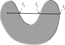
Figure 1: Ray in nonconvex body

For each such ray instead of Eq. (4) for the calculation of the energy absorbed inside the nonconvex body an expression

$$\int_{0}^{l_{1}}\!\!\varphi(x)dx+\int_{l_{2}}^{l_{3}}\!\!\varphi(x)dx=I_{\varphi}(l_{1})-I_{\varphi}(l_{2})+I_{\varphi}(l_{3})$$ (5)

should be used, where $I_{\varphi}$ is the antiderivative of $\varphi$ defined by Eq. (4). It is possible to introduce few distributions $\iota_{k}(l)$ of distances from the source to $k$-th intersection and to write instead of Eq. (3)

$$\mathfrak{D}_{B}(\varphi) = V_{B}\sum_{k=1}^{k_{\max}}(-1)^{k+1}\int_{0}^{\infty}\!\!\!\!\iota_{k}(l)\Bigl{(}\int_{0}^{l}\!\!\varphi(x)dx\Bigr{)}dl$$ (6)

$$= V_{B}\int_{0}^{\infty}\Bigl{[}\sum_{k=1}^{k_{\max}}(-1)^{k+1}\iota_{k}(l)\Bigr{]}\Bigl{(}\int_{0}^{l}\!\!\varphi(x)dx\Bigr{)}dl,$$

where $k_{\max}$ is the maximal number of intersections of a ray with the boundary of $B$. The alternating sum in square brackets in Eq. (6) may be considered as a “quasi-probability distribution” $\tilde{\iota}(l)$ and so Eq. (6) may be rewritten to produce an analogue of Eq. (3)

$$\mathfrak{D}_{B}(\varphi)=V_{B}\int_{0}^{\infty}\!\!\!\!\tilde{\iota}(l)\Bigl{(}\int_{0}^{l}\!\!\varphi(x)dx\Bigr{)}dl,\quad\tilde{\iota}(l)=\sum_{k=1}^{k_{\max}}(-1)^{k+1}\iota_{k}(l).$$ (7)

More rigorous treatment may use so-called signed measures (charges) KolmFom instead of term quasi-probability distribution used here. Some details may be found in Ref. SCLD1, .

The visual interpretation of equations for rays above is rather informal. It was used understanding description with particles propagated along straight lines. Such a picture may create a wrong impression about impossibility to apply considered methods to more difficult models with scattering. It is not so, because the only essential condition is the possibility to use in integrals like Eq. (2) expressions depending merely on $|\bm{r}_{1}-\bm{r}_{2}|$.

An example of appropriate model is a convex body with absence of scattering, but yet another case is an arbitrary body inside the medium with indistinguishable properties. The last case ensures possibility to apply Eqs. (2, 3) and further generalizations to expressions with so-called build-up factors used in dosimetry and radiation shielding to take into account the scattering RS ; M5 . For the uniform and isotropic case such a build-up factor (for given energy) is again depending only on the distance from a point source.

Let us introduce polar coordinates in the second integral in left-hand side of Eq. (2). It makes the consideration more rigour Dir1 . Then for a convex body $B$ it is possible to write

$$\mathfrak{D}_{B}(\varphi)=\int_{B}d{\mathbf{V}}_{1}\int_{0}^{\pi}\!\!\sin\theta d\theta\int_{0}^{2\pi}\!\!\!d\phi\!\int_{0}^{l(\bm{r}_{1},\theta,\phi)}\frac{\varphi(R)}{4\pi}dR,$$ (8)

where with the preceding notation of Eq. (2) $R=|\bm{r}_{1}-\bm{r}_{2}|$ together with $\theta,\phi$ are polar coordinates of the vector $\bm{R}=\bm{r}_{2}-\bm{r}_{1}$ and $l(\bm{r}_{1},\theta,\phi)$ is the length of a ray from a point $\bm{r}_{1}$ with a direction given by the polar angles $\theta$ and $\phi$.

A designation $d\Omega=\sin\theta\,d\theta\,d\phi$ for the integration on the solid angle, $\Omega$ may be used for brevity

$$\mathfrak{D}_{B}(\varphi)=\int_{B}d{\mathbf{V}}_{1}\int_{\mathbf{S}}\frac{d\Omega}{4\pi}\!\int_{0}^{l(\bm{r}_{1},\mathbf{\Omega})}\!\!\!\!\varphi(R)dR,$$ (9)

where $l(\bm{r}_{1},\mathbf{\Omega})$ is the length of a ray from a point $\bm{r}_{1}$, i.e. $\mathbf{\Omega}$ denotes direction, represented earlier via $\theta$, $\phi$.

Equation (3) may be now derived, if to take into account normalizing multipliers $V_{B}$ (volume of body $B$) and $4\pi$ (area of surface of unit sphere). It is explained below in Sec. III. Some additional technical discussion and references may be also found in Ref. SCLD1, . Here is important to emphasize, that the ray in Eq. (9) is not necessary a particle trajectory, but a formal “axis” $\bm{R}$ of the integration on the variable $R$.

Moreover, the formulas such as Eq. (5) or Eq. (6) with integrals on few disjoint intervals for a nonconvex body are also appropriate here and so Eq. (7) is valid. It justifies application of considered methods for arbitrary isotropic uniform media, i.e. for models with scattering.

The important example is a body (convex or nonconvex) inside an environment with identical or similar properties. In such a case the term in the left-hand side of Eq. (2) depends only on distance $|\bm{r}_{1}-\bm{r}_{2}|$ even for points $\bm{r}_{2}$ near the boundary. For a convex body with straight tracks it is also true, but the environment does not matter, because trajectories of particles between two points inside the body may not fall outside the boundaries unlike the case with scattering.

II.2 Method Monte Carlo with rays

A useful application of Eqs. (2, 3) is the Monte Carlo calculation of integrals. There is an additional advantage for the calculation of such integrals with many different $\varphi(l)$ for each body. In such a case CLD or RLD for given body is calculated only once and used further with different functions $\varphi(l)$. Functions, expressed via the definite integrals (single or double) of $\varphi(l)$ in right-hand side of the equations may be calculated either numerically or analytically.

The Monte Carlo sampling of a distribution is a standard procedure and may be visually represented as some histogram. The space between zero and the maximal possible length is divided on $n$ bins, i.e. sections $l_{j}\leq l<l_{j}+\Delta l$, $j=0,\ldots,n-1$ and during simulation for each step an amount of “hits” in an appropriate bin is increased by one. For the equal size $\Delta l$ of all sections the index $j$ of a bin is simply the integer part of $l/\Delta l$ and the tracing of such a data in the Monte Carlo simulations is fairly fast and useful procedure.

For the application of Eq. (7) it is possible instead of construction of $k_{\max}$ different distributions to create $\tilde{\iota}(l)$ at once. If a ray intersects boundary in few points it is necessary to consider intervals from the origin to all points of intersection. For the length of each interval with odd index (first, third, etc.) it is necessary to add unit to number of hits in a bin, but for interval with even index it is necessary to subtract unit from a number in the relevant bin.

Such a method describes the Monte Carlo algorithm for the generation of the function $\tilde{\iota}(l)$. More difficult algorithms for quasi-probability distributions of chords are discussed below. However, it is reasonable at first to recollect some concepts for the explanation, why such algorithms are relevant with alternative definitions via derivatives of the autocorrelation function.

III Helpful analytical equations

There are few functions related with presented models. It was already mentioned the chord length (distribution) density $\mu(l)$, the ray length (distribution) density $\iota(l)$, and the autocorrelation function, denoted further as $\gamma(l)$. It is also convenient to consider the probability density of the distance distribution (DD) $\eta(l)$. There are important relations between these functions Gil00 ; MRG03 ; MRD03 ; BR01 ; Str01 ; Han03 ; TorLu93 ; SCLD1 ; Kel71 ; Maz03

$$\mu(l) = \frac{\bar{l}}{V_{B}}\gamma^{\prime\prime}(l),$$ (10)

$$\mu(l) = -\bar{l}\,\iota^{\prime}(l)$$ (11)

$$\iota(l) = -\frac{1}{V_{B}}\gamma^{\prime}(l),$$ (12)

$$\eta(l) = \frac{4\pi l^{2}}{V_{B}^{2}}\gamma(l),$$ (13)

where $V_{B}$ is the volume of body $B$ and $\bar{l}=\int_{0}^{\infty}{l\,\mu(l)dl}$ is the average chord length, that may be found for a convex body from a widely used Cauchy relationship Dir1 ; Kel71 ; Ken ; San ; Cau

$$\bar{l}=4\frac{V_{B}}{S_{B}}.$$ (14)

The autocorrelation function $\gamma(l)$ is defined here for body with density $\rho(\bm{r})=1$ for $\bm{r}\in B$ as

$$\gamma(\bm{r})=\int_{B}\rho(\bm{r}_{1})\rho(\bm{r}_{1}+\bm{r})d\mathbf{V}_{1},\quad\gamma(l)=\frac{1}{4\pi l^{2}}\int_{|\bm{r}|=l}\gamma(\bm{r})d\Omega,$$ (15)

i.e. $d\mathbf{V}_{1}=dx_{1}dy_{1}dz_{1}$, $\bm{r}_{1}=(x_{1},y_{1},z_{1})$ and $\gamma(l)$ is the average of $\gamma(\bm{r})$ on a sphere with radius $l$. Definition of $\gamma$ here is lack of $1/V_{B}$ multiplier in comparison with some other works SCLD1 and it causes an insignificant difference in few equations. In fact, only the property Eq. (13) is used further and the formal definition Eq. (15) is presented here for completeness.

The probability density of the distance distribution $\eta(l)$ is easily defined for convex, nonconvex cases, and also for a system of two bodies. For the explanation of relations between derivatives of $\gamma$ in Eqs. (10, 12) it is convenient to start with the expression

$$\frac{1}{V_{B}^{2}}\mathfrak{D}_{B}(\varphi)=\frac{1}{V_{B}^{2}}\int_{B}\int_{B}\frac{\varphi(|\bm{r}_{1}-\bm{r}_{2}|)}{4\pi|\bm{r}_{1}-\bm{r}_{2}|^{2}}d{\mathbf{V}}_{1}d{\mathbf{V}}_{2}=\int_{0}^{\infty}\frac{\varphi(l)}{4\pi l^{2}}\,\eta(l)dl.$$ (16)

It may be explained using a statistical approach convenient here due to discussion on the Monte Carlo sampling. The left-hand side of Eq. (16) may be considered as an average of a function $\Phi(R)=\varphi(R)/(4\pi R^{2})$ of a variable $R=|\bm{r}_{1}-\bm{r}_{2}|$ defined on a space $B\times B$.

The multiplier $V_{B}^{2}$ is a measure (6D volume) of the six-dimensional space $B\times B$ and the division on this value is due to averaging. On the other hand, the standard correspondence SkorPro of a stochastic average with a mathematical expectation $\mathbf{E}$ makes possible to use the formula

$$\mathbf{E}\Phi(R)=\int\Phi(l)\,d_{l}F_{R}(l),$$ (17)

where $F_{R}(l)$ is the cumulative distribution function of a random variable $R$ and $d_{l}F_{R}(l)$ denotes probability density of $R$, but in the considered case it is just the density of the distances distribution (DD) defined earlier $\eta(l)dl=d_{l}F_{R}(l)$. Really, $R$ is the distance between two points $\bm{r}_{1}$, $\bm{r}_{2}$ with independent uniform distributions and double integral in Eq. (16) corresponds to averaging on $B\times B$ for such a pair.

Equation (16) may be rewritten due to relation Eq. (13) as

$$\mathfrak{D}_{B}(\varphi)=\int_{0}^{\infty}\!\!\!\varphi(l)\,\gamma(l)dl.$$ (18)

After integration by parts it is possible to obtain from Eq. (18)

$$\mathfrak{D}_{B}(\varphi)=\int_{0}^{\infty}\!\!\!\![-\gamma^{\prime}(l)]\Bigl{(}\int_{0}^{l}\!\!\varphi(x)dx\Bigr{)}dl.$$ (19)

For a convex body Eq. (19) is in agreement with Eqs. (3, 12).

Equation (3) may also be proven using an analogue of the statistical approach discussed above. A detailed proof may be found elsewhere SCLD1 and is only briefly sketched here. It is possible to consider Eq. (9) as an averaging on the five-dimensional space of rays, represented as product $B\times{\mathbf{S}}$ of the body $B$ on the unit sphere ${\mathbf{S}}$. It is necessary to use for normalization the volume $V_{B}$ of $B$ multiplied on $4\pi$, the surface area of the unit sphere. In such a case Eq. (3) may be considered as an analogue of Eq. (17) for the mathematical expectation of some function depending on the length of a ray.

It is possible to derive an equivalent of Eq. (12) for a nonconvex body with $\tilde{\iota}(l)$ introduced in Eq. (7) if to use generalized functions and derivatives. The idea of a generalized function is convenient also for the further work with integrals such as $\mathfrak{D}(\varphi)$.

The generalized function (distribution) is defined KolmFom as the continuous linear functional $\mathfrak{T}(\phi)$ on the space of test functions $\phi$. Usual integrable function $\psi$ may be associated with a functional $\mathfrak{T}_{\psi}$ defined for the test function $\phi(x)$ as

$$\mathfrak{T}_{\psi}(\phi)=\int_{-\infty}^{\infty}\psi(x)\phi(x)dx.$$ (20)

On the other hand, $\mathfrak{D}_{B}:\varphi\to\mathfrak{D}_{B}(\varphi)$ is also a linear functional on a test function $\varphi$ and may be considered as some generalized function on $(0,\infty)$ defined by given body $B$. A topology on the space of test functions and continuityKolmFom , i.e. $\mathfrak{D}_{B}(\varphi_{k})\to\mathfrak{D}_{B}(\varphi)$ for $\varphi_{k}\to\varphi$, are not discussed here.

It is often used as a simplified notation $\psi$ instead of $\mathfrak{T}_{\psi}$ for such a regular generalized function Eq. (20) KolmFom . In such a case Eq. (18) may be rewritten simply as $\mathfrak{D}_{B}=\gamma_{B}$.

The generalized derivative KolmFom is defined as functional

$$\mathfrak{T}^{\prime}(\phi)=-\mathfrak{T}(\phi^{\prime}).$$ (21)

Due to Eq. (3) it is possible for convex body $B$ to write $\mathfrak{D}_{B}^{\prime}=-V_{B}\,\iota_{B}$ and Eq. (7) for an arbitrary body ensures $\mathfrak{D}_{B}^{\prime}=-V_{B}\,\tilde{\iota}_{B}$.

IV Chord method

IV.1 Chord length distribution

For a convex body Eq. (2) may be rewritten with generalized functions and derivatives as $\mathfrak{D}_{B}^{\prime\prime}=(S_{B}/4)\mu_{B}$. Here generalized functions may be more appropriate, because due to the expression with the second derivative CLD is not a regular function even if DD is not smooth in some points.

Formally, for a convex body an expression with an additional integration along a chord appears due to a rearrangement of the integral Eq. (8) and consideration of all possible rays with origins along the same chord Dir1 (see Fig. 2).

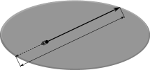
Figure 2: Consideration of all possible rays along a chord

If to use a compact notation $\int d\mathcal{L}$ for the formal integration on a four-dimensional space of straight lines Ken ; San , it is possible to rewrite Eq. (9) after such a rearrangement as

$$\mathfrak{D}_{B}(\varphi)=\int\frac{d{\mathcal{L}}}{4\pi}\int_{0}^{l(\mathcal{L})}\!\!\!\int_{0}^{r}\!\!\varphi(x)dx\,dr,$$ (22)

where $l(\mathcal{L})$ is the length of a chord produced by the intersection of the straight line $\mathcal{L}$ with the convex body $B$. Equation (22) is an analogue of a familiar expression used for the derivation of the Dirac’s chord method (see Eq. (1.5) in Ref. Dir1, ).

In such a case there is a double integral along a chord due to the additional integration on sources of rays

$$I^{(2)}_{\varphi}(l)=\int_{0}^{l}\!\!\int_{0}^{r}\!\!\varphi(x)dx\,dr.$$ (23)

For a nonconvex body and few chords, i.e. $n$ intervals of intersections $[x_{2k},x_{2k+1}]$, $k=0,\ldots n-1$ of the body by the same straight line, it is necessary to include only the integration on both “source” points $r$ and “target” points $r_{2}=r+x$ inside these intervals. Using rather technical calculation (see Ref. SCLD1, , Sec 3.3) it is possible to obtain instead of Eq. (23) the more difficult expression

$$I^{(2)}_{\varphi}(x_{0},\ldots,x_{2n-1}) = \sum_{k=0}^{n-1}I^{(2)}_{\varphi}(x_{2k+1}-x_{2k})$$ (24)

$$+ \sum_{k=1}^{n-1}\sum_{j=0}^{k-1}[I^{(2)}_{\varphi}(x_{2k+1}-x_{2j})+I^{(2)}_{\varphi}(x_{2k}-x_{2j+1})]$$

$$- \sum_{k=1}^{n-1}\sum_{j=0}^{k-1}[I^{(2)}_{\varphi}(x_{2k+1}-x_{2j+1})+I^{(2)}_{\varphi}(x_{2k}-x_{2j})].$$

It includes all $n(2n-1)$ possible ordered pairs $x_{k}-x_{j}$ with indexes $0\leq j<k\leq 2n-1$ and may be rewritten as

$$I^{(2)}_{\varphi}(x_{0},\ldots,x_{2n-1})=\sum_{k=1}^{2n-1}\sum_{j=0}^{k-1}(-1)^{k-j+1}I^{(2)}_{\varphi}(x_{k}-x_{j}).$$ (25)

E.g., for two intersections there are six terms (see Fig. 3)

$$I^{(2)}_{\varphi}(x_{0},\ldots,x_{3})=I^{(2)}_{\varphi}(x_{1}-x_{0})+I^{(2)}_{\varphi}(x_{3}-x_{2})$$

$$\qquad+I^{(2)}_{\varphi}(x_{3}-x_{0})+I^{(2)}_{\varphi}(x_{2}-x_{1})-I^{(2)}_{\varphi}(x_{2}-x_{0})-I^{(2)}_{\varphi}(x_{3}-x_{1}).$$

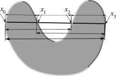
Figure 3: Chords in nonconvex body and six possible segments

Let us rewrite the integral Eq. (22)

$$\mathfrak{D}_{B}(\varphi)=\int\frac{d\mathcal{L}}{4\pi}I^{(2)}_{\varphi}(\mathcal{L}),$$ (26)

where for a convex body due to Eq. (23) $I^{(2)}_{\varphi}(\mathcal{L})=I^{(2)}_{\varphi}(l_{\mathcal{L}})$. The same expression also may be used for a nonconvex body if to denote $I^{(2)}_{\varphi}(\mathcal{L})=I^{(2)}_{\varphi}(x^{\mathcal{L}}_{0},\ldots,x^{\mathcal{L}}_{2n-1})$, where $x^{\mathcal{L}}_{0},\ldots,x_{2n-1}^{\mathcal{L}}$ designate all intersections of the straight line $\mathcal{L}$ with the boundary of $B$.

On the other hand, $I^{(2)}_{\varphi}(\mathcal{L})$ may be expressed as a sum Eq. (25) with all possible (ordered) pairs of points. It is possible to rewrite Eq. (26) for the nonconvex case

$$\mathfrak{D}_{B}(\varphi)=\int\frac{d\mathcal{L}}{4\pi}\sum_{k=1}^{2n-1}\sum_{j=0}^{k-1}(-1)^{k-j+1}I^{(2)}_{\varphi}(x^{\mathcal{L}}_{k}-x^{\mathcal{L}}_{j}).$$ (27)

The situation is similar with expressions for rays in a nonconvex body Eqs. (6, 7). Let us denote as $\mu_{jk}(l)$ probability densities of distributions of lengths $l_{jk}=x^{\mathcal{L}}_{k}-x^{\mathcal{L}}_{j}$ produced by $n(2n-1)$ ordered pairs $(x^{\mathcal{L}}_{j},x^{\mathcal{L}}_{k})$ on a line $\mathcal{L}$.

If to introduce

$$\tilde{\mu}_{tot}(l)=\sum_{k=1}^{2n-1}\sum_{j=0}^{k-1}(-1)^{k-j+1}\mu_{jk}(l),\quad\tilde{\mu}=\tilde{m}^{-1}\tilde{\mu}_{tot}(l),$$ (28)

where $\tilde{m}$ is the normalization

$$\tilde{m}=\int_{0}^{\infty}\tilde{\mu}_{tot}(l)dl,$$ (29)

it is possible to write an analogue of Eq. (2) for a nonconvex body $B$

$$\mathfrak{D}_{B}(\varphi)=\tilde{s}_{B}\int_{0}^{\infty}\!\!\!\!\tilde{\mu}(l)I_{\varphi}^{(2)}(l)dl=\tilde{s}_{B}\int_{0}^{\infty}\!\!\!\!\tilde{\mu}(l)\Bigl{(}\int_{0}^{l}\!\!\int_{0}^{r}\!\!\varphi(x)dx\,dr\Bigr{)}dl,$$ (30)

where $\tilde{s}_{B}$ is some constant.

For a convex body $\tilde{\mu}(l)=\mu(l)$, $\tilde{s}_{B}=S_{B}/4$ and Eq. (30) may be explained using an idea with the averaging and the mathematical expectation Eq. (17) already discussed for DD and RLD. Let us consider an average of the function $f(\mathcal{L})=I^{(2)}_{\varphi}(l_{\mathcal{L}})$ on the four-dimensional set $\mathcal{L}[B]$ of all straight lines intersecting the body $B$

$$\frac{1}{w_{B}}\int_{\mathcal{L}[B]}\!\!I^{(2)}_{\varphi}(l_{\mathcal{L}})d\mathcal{L}=\int_{0}^{\infty}\!\!\!\!I_{\varphi}^{(2)}(l)\mu(l)dl,$$ (31)

where $w_{B}$ is a measure (4D volume) of $\mathcal{L}[B]$. For a convex body it may be expressed as $w_{B}=\pi S_{B}$ due to a Cauchy relationship SCLD1 ; Ken ; San ; Cau ; Mat ; Helg and after comparison of Eq. (31) with Eq. (22) we obtain necessary coefficient $w_{B}/(4\pi)=S_{B}/4$ used in Eq. (2).

For a nonconvex body there are $n(2n-1)$ distributions $\mu_{jk}(l)$ instead of one and Eq. (30) is obtained via the alternating sum Eq. (27) of these distributions and so formula $\tilde{s}_{B}=\tilde{m}_{B}^{-1}w_{B}/(4\pi)$ is valid with $w_{B}$ is a measure for a set of all straight lines intersecting $B$ and $\tilde{m}_{B}$ is a constant used in definition of $\tilde{\mu}(l)$ Eq. (28). The problem here is an absence of simple methods of a calculation $w_{B}$ and $\tilde{m}_{B}$ for nonconvex bodies and so it may be convenient to consider yet another approach for finding $\tilde{s}_{B}$.

It is possible to use an analogue of the relation in Eq. (11). The integration by parts of Eq. (7) for a nonconvex body produces

$$\mathfrak{D}_{B}(\varphi)=V_{B}\int_{0}^{\infty}\!\!\!\![-\tilde{\iota}^{\prime}(l)]\Bigl{(}\int_{0}^{l}\!\!\int_{0}^{r}\!\!\varphi(x)dx\,dr\Bigr{)}dl$$ (32)

and after the comparison with Eq. (30) it is possible to write

$$-V_{B}\tilde{\iota}^{\prime}(l) = \tilde{s}_{B}\tilde{\mu}(l)$$

$$-V_{B}\int_{0}^{\infty}\!\!l\,\tilde{\iota}^{\prime}(l)dl = \tilde{s}_{B}\int_{0}^{\infty}\!\!l\,\tilde{\mu}(l)dl$$

$$V_{B}\int_{0}^{\infty}\!\!\tilde{\iota}(l)dl = \tilde{s}_{B}\bar{l}\int_{0}^{\infty}\!\!\tilde{\mu}(l)dl,$$

where by definition $\bar{l}_{B}=\int l\tilde{\mu}_{B}(l)dl/\!\int\tilde{\mu}_{B}(l)dl$ and due to normalization of $\tilde{\iota}(l)$ and $\tilde{\mu}(l)$

$$\tilde{s}_{B}=V_{B}/\bar{l}_{B}.$$ (33)

For a convex body $\bar{l}_{B}$ is the average chord length. For a nonconvex body it is equal to the average chord length for the multi-chord distribution (MCD) mentioned earlier, because sums of lengths of all intervals in two last terms of Eq. (24) compensate each other SCLD1 . It is clarified below in Sec. IV.2 about Monte Carlo simulations.

In fact, the Cauchy relationship Eq. (14) for the average chord length for MCD is proved for a broad class of nonconvex bodies MRG03 and so it is also possible to write due to Eq. (33) in such a case

$$\tilde{s}_{B}=S_{B}/4.$$ (34)

For numerical methods using Eq. (33) with $\bar{l}_{B}$ sometimes may be preferable. It is instructive to consider an example with so-called voxel presentation of a body as a decomposition on small cubes or parallelepipeds. In such a case the surface is not smooth and a problem with correct approximation of surface area may not be resolved even for a formal limiting case with cubes of arbitrary small dimensions, e.g. for a sphere such a limit is $6\pi r^{2}$ instead of surface area $4\pi r^{2}$.

IV.2 Method Monte Carlo with chords

Let us consider some questions of the Monte Carlo generation of the quasi-probability distribution $\tilde{\mu}(l)$. For each straight line with $n>1$ intervals inside a body $B$ it is necessary to consider $2n$ points of intersection with the boundary of $B$. Tangent points should be counted twice. Let us mark all points by real numbers $x_{k}$, $k=0,\ldots,2n-1$, there $x_{0}=0$ and other $x_{k}$ denote distances along a given straight line, i.e. $x_{k}=|\bm{r}_{k}-\bm{r}_{0}|$, where $\bm{r}_{k}$ denote positions of $2n$ points of intersections in the three-dimensional space.

It is clear from further consideration that it is possible to use opposite order of points $\bm{r}_{k}\leftrightarrow\bm{r}_{2n-k-1}$ and so “$\pm$ orientation” of a line does not matter, i.e. two opposite directions could not be distinguished. Anyway, in applied calculations it is often more convenient to use directed lines. Standard algorithms of the generation of uniform isotropic (pseudo)random sequences of straight lines should be discussed elsewhere.

Let us discuss the procedure of the construction of $\tilde{\mu}(l)$ for the given line. If the line intersects a body $n$ times, it is necessary to consider set of $2n$ numbers $x_{k}$ defined above and to calculate lengths $l_{jk}=(x_{k}-x_{j})$ for all $j,k:0\leq j<k\leq 2n-1$.

For given $l_{jk}$ a number in the relevant bin should be increased by unit for odd $k-j$ and decreased by unit otherwise, i.e. if $k-j$ is even. For $2n$ indexes there are $1+2+\cdots+(2n-1)=n(2n-1)$ ordered pairs. Between them $n$ pairs $(x_{2k},x_{2k+1})$, $k=0,\ldots,n-1$ represent usual chords lying completely inside the body and they have positive contributions.

Remaining $n(2n-2)$ pairs are not forming intervals entirely belonging to the body and may be divided in two equal groups. There are $n(n-1)$ pairs with positive contribution, i.e. $(x_{2j},x_{2k+1})$ or $(x_{2j+1},x_{2k})$, $0\leq j<k\leq n-1$. For other $n(n-1)$ pairs, i.e. $(x_{2j},x_{2k})$ or $(x_{2j+1},x_{2k+1})$, $0\leq j<k\leq n-1$, numbers in appropriate bins should be decreased.

It is also clear from such a representation why sums of lengths of the pairs in two last groups compensate each other:

$$(x_{2k+1}-x_{2j})+(x_{2k}-x_{2j+1})=(x_{2k}-x_{2j})+(x_{2k+1}-x_{2j+1}).$$

So sum of lengths alternating in signs is equal with summation of only $n$ positive contributions due to chords of the straight line inside the body.

There is also additional subtlety with normalization. For each straight line the total increase of values in all affected bins is

$$\Delta N_{tot}=n+n(n-1)-n(n-1)=n.$$

So there are two different counters: the number of lines $N_{l}$ and the sum of numbers in all bins $N_{tot}\geq N_{l}$, which is equivalent with a total number of separate chords lying completely inside the body. The (quasi-probability) distribution should be divided in $N_{tot}$ for normalization. It is similar with the multi-chord distribution (MCD), because it is also normalized on the same number of separate chords $N_{tot}$.

It was shown above that total sum of all lengths while taking into account signs is equal with sum of chords inside the body. But the normalization is the same as for MCD case and so the formal averaging of the variable $l$ for the quasi-probability distribution $\tilde{\mu}(l)$ constructed here is the same as the average chord length for MCD that could be produced from the same set of straight lines. In a limit $N_{l}\to\infty$ it ensures equality of $\bar{l}$ for both distributions already mentioned and used above in Eq. (34).

The total number of lines $N_{l}$ corresponds to the normalization for OCD case, when for each straight line only one “aggregated” chord, equivalent to union of all chords inside a nonconvex body, is considered. $N_{l}$ is also related with measure of set of all straight lines intersecting the considered body. Earlier in Eq. (31) this measure was denoted as $w_{B}$.

Yet another application of the both $N_{tot}$ and $N_{l}$ is the calculation of a constant $\tilde{m}$ used earlier in Eq. (28). It may be expressed as a relation between $\tilde{\mu}_{tot}$ (that is not normalized on unit due to the contribution of lines intersecting the body more than one time) and $\tilde{\mu}$. So $\tilde{m}$ is the limit of ratio between total number of chords $N_{tot}$ (cf MCD) and total number of straight lines $N_{l}$ (cf OCD)

$$\tilde{m}=\lim_{N_{l}\to\infty}N_{tot}/N_{l}.$$ (35)

V Multi-body case

V.1 Some equations with two different bodies

This section is devoted to initial question about the calculation of the integral Eq. (1) with two different bodies. Here, it is also convenient to consider a simple model with particles moving along straight lines in isotropic uniform medium and to use the interpretation of Eq. (1) as a fraction of energy emitted in $B_{1}$ and absorbed in $B_{2}$.

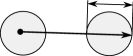
Figure 4: Ray from $B_{1}$ with interval inside of $B_{2}$

Let us consider a particle emitted in the first body with the straight trajectory intersecting the second one (Fig. 4). If the law of absorption is the same in both bodies and medium between them, it is possible to describe amount of energy absorbed in the second body as

$$\int_{a}^{b}\!\!\varphi(x)dx=I_{\varphi}(b)-I_{\varphi}(a),$$ (36)

where $a$ and $b$ are distances from a source to two intersections of second body by the ray and $I_{\varphi}$ is defined above in Eq. (4).

Calculation of Eq. (1) for a convex $B_{2}$ would be related with an analogue of Eq. (8)

$$\mathfrak{F}_{B_{1}}^{B_{2}}(\varphi)=\int_{B_{1}}d{\mathbf{V}}_{1}\int_{\theta_{\min}(\bm{r}_{1},\phi)}^{\theta_{\max}(\bm{r}_{1},\phi)}\!\!\sin\theta d\theta\int_{\phi_{\min}(\bm{r}_{1})}^{\phi_{\max}(\bm{r}_{1})}\!\!\!d\phi\!\int_{a(\bm{r}_{1},\theta,\phi)}^{b(\bm{r}_{1},\theta,\phi)}\frac{\varphi(R)}{4\pi}dR,$$ (37)

where $\theta_{\min},\theta_{\max},\phi_{\min},\phi_{\max}$ describe angular limits of integrations for given point $\bm{r}_{1}$ and $a$, $b$ are radial distances for given point and direction. It maybe simpler to use an analogue of Eq. (9)

$$\mathfrak{F}_{B_{1}}^{B_{2}}(\varphi)=\int_{B_{1}}d{\mathbf{V}}_{1}\int_{{\mathbf{S}}(\bm{r}_{1},B_{2})}\!\frac{d\Omega}{4\pi}\!\int_{a(\bm{r}_{1},\mathbf{\Omega})}^{b(\bm{r}_{1},\mathbf{\Omega})}\!\!\!\varphi(R)dR,$$ (38)

where ${\mathbf{S}}(\bm{r}_{1},B_{2})$ is central projection from point $\bm{r}_{1}$ of body $B_{2}$ to surface of unit sphere. Yet, an alternative method of calculations is presented further and Eqs. (37, 38) are mentioned here rather for some clarification and comparison.

V.2 Relation with methods for single body

For two nonconvex bodies expressions above could be even more difficult, but it is possible to use a general principle to adapt already developed approach with single body SCLD2 . Let us choose both bodies as sources and consider four integrals $\mathfrak{F}_{B_{s}}^{B_{t}}(\varphi)$, $s=1,2$, $t=1,2$, i.e. $\mathfrak{F}_{B_{1}}^{B_{1}}=\mathfrak{D}_{B_{1}}$, $\mathfrak{F}_{B_{2}}^{B_{2}}=\mathfrak{D}_{B_{2}}$, $\mathfrak{F}_{B_{1}}^{B_{2}}=\mathfrak{F}_{B_{2}}^{B_{1}}$. Each integral takes into account only particles emitted in $B_{s}$ and absorbed in $B_{t}$.

The double integrals Eqs. (1, 2) comply with simple relations

$$\mathfrak{D}_{B_{1}\cup B_{2}}(\varphi)=\mathfrak{F}_{B_{1}}^{B_{1}}(\varphi)+\mathfrak{F}_{B_{1}}^{B_{2}}(\varphi)+\mathfrak{F}_{B_{2}}^{B_{1}}(\varphi)+\mathfrak{F}_{B_{2}}^{B_{2}}(\varphi)$$ (39)

and

$$2\mathfrak{F}_{B_{1}}^{B_{2}}(\varphi)=\mathfrak{D}_{B_{1}\cup B_{2}}(\varphi)-\mathfrak{D}_{B_{1}}(\varphi)-\mathfrak{D}_{B_{2}}(\varphi).$$ (40)

So many equations with two bodies may be reduced to already discussed case with the single body using union of these bodies $B=B_{1}\cup B_{2}$.

Here it is suggested that $B_{1}$ does not intersect $B_{2}$. For overlapping bodies the decomposition on three parts: $B_{1}\cup B_{2}$, $B_{1}\setminus B_{2}$ and $B_{2}\setminus B_{1}$ should be taken into account. Instead of Eq. (40) in such a case a modified expression may be used:

$$2\mathfrak{F}_{B_{1}}^{B_{2}}(\varphi)=\mathfrak{D}_{B_{1}\cup B_{2}}(\varphi)+\mathfrak{D}_{B_{1}\cap B_{2}}(\varphi)-\mathfrak{D}_{B_{1}}(\varphi)-\mathfrak{D}_{B_{2}}(\varphi).$$ (41)

Due to such equations, the computational methods discussed above make possible to find Eq. (1) after separate calculations of three or four terms in Eq. (40) or Eq. (41). However, more direct approach discussed further is also useful and may be simply generalized for the case with many bodies.

A simpler case of two disjoint bodies is suitable for almost straightforward modifications of Monte Carlo algorithms discussed above SCLD2 . Here Eq. (39) demonstrates that distributions obtained in simulation may be divided in four parts (for each pair source-target) without significant modification of algorithms for general nonconvex body discussed above and it may be even more convenient for explanation than Eq. (40).

For two discontiguous bodies a union $B=B_{1}\cup B_{2}$ formally is always nonconvex, because a line between a point in $B_{1}$ and a point in $B_{2}$ lies partially outside the union. So, here, consideration of quasi-probability distributions is especially justified.

For non-overlapping bodies with adjoining boundaries $B$ may be convex even with nonconvex $B_{1}$ or $B_{2}$. It corresponds to the case briefly mentioned below in a note about zones at the end of Sec. V.4. It is enough to consider some body $B$ and formally split it into two zones (parts) $B_{1}$ and $B_{2}$. Even for convex body such parts may be either convex or nonconvex. These subtleties do not affect on methods discussed here. Insignificant change is necessary only for a case with overlapping bodies due to contribution of intersections with nonzero volume outlined in Eq. (41).

V.3 Application to calculations with rays

Source points uniformly distributed in both bodies with equivalent density are used for sampling with rays. All intersections of rays with boundaries of both bodies are checked and appropriate bins are changed in four histograms $H_{st}(l)$ marked by indexes source-target.

Joint consideration of all distributions lets to tackle a problem with normalization. For the function $\tilde{\iota}$ term “quasi-probability distribution” could be justified due to normalization on unit integral and some relations with the probability density for length of rays in a convex body, but if to write an analogue of Eq. (3) for the integral Eq. (1)

$$\mathfrak{F}_{B_{1}}^{B_{2}}(\varphi)=W_{12}\int_{0}^{\infty}\!\!\!\!\tilde{\iota}_{(12)}(l)\Bigl{(}\int_{0}^{l}\!\!\varphi(x)dx\Bigr{)}dl,$$ (42)

where $W_{12}$ is an unknown constant, it is simple to show that $\tilde{\iota}_{(12)}(l)$ may not be normalized for disjoint bodies, because due to Eq. (40)

$$W_{12}\int_{0}^{\infty}\!\!\tilde{\iota}_{(12)}(l)dl=(V_{1}+V_{2})\int\!\!\tilde{\iota}_{\cup}(l)dl-V_{1}\int\!\!\tilde{\iota}_{1}(l)dl-V_{2}\int\!\!\tilde{\iota}_{2}(l)dl=0,$$

where integrals of all functions $\tilde{\iota}_{1}(l)$, $\tilde{\iota}_{2}(l)$ and $\tilde{\iota}_{\cup}(l)=\tilde{\iota}_{B_{1}\cup B_{2}}(l)$ are normalized on unit.

However, if to include all four densities as components in the single process described by a (quasi-probability) distribution, introduced earlier

$$\tilde{\iota}_{\cup}(l)=\sum_{s,t}\tilde{\iota}_{(st)}(l),$$ (43)

it is possible to consider $\tilde{\iota}_{(st)}(l)$ as elements of some matrix $\mathbf{\tilde{\iota}}(l)$ with the common normalization. The same approach may be used for more than two bodies.

V.4 Application to calculations with chords

The expression of Eq. (1) via chord distributions also may use similar principles SCLD2 . Here, it is also appropriate to use the decomposition Eq. (39). A straight line again determines $2n$ values $x_{0},\ldots,x_{2n-1}$, but boundaries of both bodies must be marked appropriately. Each intersection should be refined as $x_{k}^{s}$ with additional index $s=1,2$ for $B_{1}$, $B_{2}$.

Each pair $(x_{j}^{s},x_{k}^{t})$ already has two additional indexes $s$ and $t$ representing four possible combinations for two bodies and it produces distributions $\mu^{(st)}_{jk}(l)$ combined with appropriate signs $(-1)^{k+j-1}$ into $\tilde{\mu}_{(st)}(l)$, $s,t=1,2$. It should be only mentioned that due to a symmetry for the chords “source” and “target” bodies could be hardly distinguished. Due to such property it is reasonable to use only three separate histograms $H_{11}$, $H_{22}$ and $H_{12}+H_{21}$ and to define $\tilde{\mu}_{\{st\}}(l)$ as a symmetric matrix.

It may be directly generalized for a case with $m$ bodies with $s,t=1,\ldots,m$. Advantages of application of discussed methods may be illustrated by consideration of a domain with many different bodies intersected by the variety of straight lines. It is possible to calculate all $m^{2}$ integrals $\mathfrak{F}_{B_{s}}^{B_{t}}$ during the same Monte Carlo simulation.

Here only $m(m+1)/2$ integrals are different due to symmetry, but anyway it may be a big number. For medical applications with $15-20$ objects (organs) it is the calculation of hundreds values in a single Monte Carlo run. In fact, speed up may be even more critical due to possibility to split each body into few zones. The subdivision may be necessary for taking into account a variation of the intensity of emitters in the different parts of some objects.

There is a subtlety for the calculation with few zones: it is necessary formally to split each boundary between two zones into two coinciding surfaces. In such a case all equations above are valid, but there are some intervals with zero length. Such intervals may be simply omitted, because integration along them produces zero values.

V.5 Analytical expressions for two bodies

There are useful analogues of expressions discussed in the Sec. III for the case with two bodies. A function $\eta_{(12)}(l)$ may be defined as the probability density of distances between a pair of points uniformly distributed in first and second body, respectively. Analytical expressions written below may be used for the testing of the Monte Carlo simulation and some clarification. Technical details may be found in Ref. SCLD2, .

The correlation function $\gamma_{(12)}(l)$ is defined for two bodies with unit densities $\rho_{k}(\bm{r})=1$ for $\bm{r}\in B_{k}$, $k=1,2$ as

$$\gamma_{(12)}(\bm{r})=\int_{B_{1}}\rho_{1}(\bm{r}_{1})\rho_{2}(\bm{r}_{1}+\bm{r})d\mathbf{V}_{1},\quad\gamma_{(12)}(l)=\frac{1}{4\pi l^{2}}\int_{|\bm{r}|=l}\gamma_{(12)}(\bm{r})d\Omega.$$ (44)

It is possible to derive the direct analogue of Eq. (13)

$${\eta}_{(12)}=\frac{4\pi l^{2}}{V_{1}V_{2}}\gamma_{(12)}(l)$$ (45)

and to write the generalization of Eq. (18)

$$\mathfrak{F}_{B_{1}}^{B_{2}}(\varphi)=\int_{0}^{\infty}\!\!\!\varphi(l)\,\gamma_{(12)}(l)dl.$$ (46)

Using integrations of Eq. (46) by parts it is possible to express $\tilde{\iota}_{(12)}$ and $\tilde{\mu}_{(12)}$ as first and second derivatives of correlation function $\gamma_{(12)}(l)$, respectively. It is similar with Eq. (12) and Eq. (10). If to use the normalization on the union of bodies suggested above and the Cauchy relationship for the average chord length Eq. (14), it may be written

$$\tilde{\mu}_{(12)}(l) = \frac{4}{S_{B_{1}}+S_{B_{2}}}\gamma^{\prime\prime}_{(12)}(l),$$ (47)

$$\tilde{\iota}_{(12)}(l) = -\frac{1}{V_{B_{1}}+V_{B_{2}}}\gamma^{\prime}_{(12)}(l).$$ (48)

Due to such normalization for the ray method an “unknown constant” in Eq. (42) may be chosen as

$$W_{12}=V_{B_{1}}+V_{B_{2}}$$ (49)

and desired generalization of the Dirac’s chord method for the initial equation Eq. (1) may be written finally as

$$\mathfrak{F}_{B_{1}}^{B_{2}}(\varphi)=\frac{S_{B_{1}}+S_{B_{2}}}{4}\int_{0}^{\infty}\!\!\!\!\tilde{\mu}_{(12)}(l)\Bigl{(}\int_{0}^{l}\!\!\int_{0}^{r}\!\!\varphi(x)dx\,dr\Bigr{)}dl.$$ (50)

VI Conclusion

A novel approach with the application of quasi-probability distributions (signed measures) to calculations of integrals such as Eqs. (1, 2) is advocated in presented work. It may be useful in many areas of physics. This paper is written with a purpose to present a fairly brief, but closed description of considered methods. Additional technical details, proofs of some equations together with appropriate links with theory of geometrical probabilities may be found elsewhere SCLD1 ; SCLD2 .

It is shown, how models with ray and chord length distributions suitable for a single convex body should be altered for a nonconvex case and multi-body systems. An essential new property of such extensions is the necessity to use instead of probability densities some functions, which sometimes do not satisfy the non-negativity condition.

Maybe such a counterintuitive “negative probability” produced certain difficulties and a delay in development and applications of these methods despite of high effectiveness of numerical algorithms based on ray and chord distributions. On the other hand, quasi-probability distributions are rather common in quantum physics after so-called Wigner function representation WigFun and Feynman wrote an essay about the concept of negative probability with reasonable examples both in quantum and classical physics FeyNeg .

In fact, the functions $\tilde{\iota}(l)$ and $\tilde{\mu}(l)$ do not necessarily directly related with probability distributions and so should not cause some conceptual challenges. Appearance of negative values may be simply illustrated using Eq. (5) and Fig. 1. Here the ray $(0,l_{3})$ includes a ray $(0,l_{1})$ already taken into account and the interval $(l_{1},l_{2})$ outside of the body, that should not be counted at all.

For the work with an interval $(l_{2},l_{3})$ expressions such as Eq. (5) were used, but it may be described in the standard probability theory. If probability measures are known for sets $R_{1}=A$, $R_{2}=A\cup B$, $R_{3}=A\cup B\cup C$, it is possible to write for $C$: ${\mathbf{P}}(C)={\mathbf{P}}(R_{3}\setminus R_{2})={\mathbf{P}}(R_{3})-{\mathbf{P}}(R_{2})$ and for $A\cup C$: ${\mathbf{P}}(A\cup C)={\mathbf{P}}(R_{1})-{\mathbf{P}}(R_{2})+{\mathbf{P}}(R_{3})$.

Overlapping sets, i.e. rays with the same origin, are used in construction of $\tilde{\iota}(l)$ (see Fig. 1). Positive and negative terms such as ${\mathbf{P}}(R_{3})$ and $-{\mathbf{P}}(R_{2})$, used for the calculation of the same ${\mathbf{P}}(C)$, affect two ranges of argument $\tilde{\iota}(l)$. So for $l=R_{3}$ there is some positive gain, but for $l=R_{2}$ there is corresponding decrease and it may produce negative values of $\tilde{\iota}(l)$ for some intervals of $l$. An extra hit is added to some bin. A removal from another bin — is an effort to compensate that, but it may produce a negative result.

The construction of $\tilde{\iota}(l)$ is simpler, than the generalization of the chord length distribution $\tilde{\mu}(l)$, but a reason of appearance of negative values in both cases is similar. An amount of terms in expressions for a ray grows linearly with respect to a number of intersections and for chord it is quadratic dependence. The structure of sets is also more complicated for chords, but here alternating signs in formulas such as Eq. (24) again correspond to an expression with unions and differences of some overlapped sets.

References

- (1) J. K. Shultis and R. E. Faw, “Radiation shielding technology,” Health Phys. 88(4), 297–322 (2005).
- (2) W. S. Snyder, M.R. Ford, and G. G. Warner, “Estimates of specific absorbed fractions for photon sources uniformly distributed in various organs of a heterogeneous phantom,” MIRD Pamplet No. 5, revised (New York, NY: Society of Nuclear Medicine, 1978).
- (3) P. A. M. Dirac, “Approximate rate of neutron multiplication for a solid of arbitrary shape and uniform density, I: General theory,” in The Collected Works of P. A. M. Dirac 1924–1948, R. H. Dalitz (ed.), 1115–1128 (Oxford University Press, Oxford, 1995).
- (4) P. A. M. Dirac, K. Fuchs, R. Peierls, and P. Preston, “Approximate rate of neutron multiplication for a solid of arbitrary shape and uniform density, II: Application to the oblate spheroid, hemisphere and oblate hemispheroid,” ibid, 1129–1145.
- (5) N. Metropolis, “The beginning of the Monte Carlo method,” Los Alamos Science 15, 125–130 (1987).
- (6) W. Gille, “Chord length distributions and small-angle scattering,” Eur. Phys. J. B 17, 371–383 (2000).
- (7) A. Mazzolo, B. Roesslinger, and W. Gille, “Properties of chord length distributions of nonconvex bodies,” J. Math. Phys. 44, 6195–6208 (2003).
- (8) A. Mazzolo, B. Roesslinger, and C. M. Diop, “On the properties of the chord length distribution, from integral geometry to reactor physics,” Ann. Nucl. Energy 30, 1391–1400 (2003).
- (9) C. Burger and W. Ruland, “Analysis of chord-length distributions,” Acta Cryst. A57, 482–491 (2001).
- (10) N. Stribeck, “Extraction of domain structure information from small-angle scattering patterns of bulk materials,” J. Appl. Cryst. 34, 496–503 (2001).
- (11) W. Gille, “Linear simulation models for real-space interpretation of small-angle scattering experiments of random two-phase systems,” Waves Random Media 12, 85–97 (2002).
- (12) S. Hansen, “Estimation of chord length distributions from small-angle scattering using indirect Fourier transformation,” J. Appl. Cryst. 36, 1190–1196 (2003).
- (13) W. Gille, A. Mazzolo, and B. Roesslinger, “Analysis of the initial slope of the small-angle scattering correlation function of a particle,” Part. Part. Syst. Charact. 22, 254–260 (2005).
- (14) S. Torquato and B. Lu, “Chord-length distribution function for two-phase random media,” Phys. Rev. E 47, 2950–2953 (1993).
- (15) A. Yu. Vlasov, “Signed chord length distribution. I,” arXiv:0711.4734 [math-ph] (2007).
- (16) A. Yu. Vlasov, “Signed chord length distribution. II,” arXiv:0904.3646 [math-ph] (2009).
- (17) A. N. Kolmogorov and S. V. Fomin, Introductory real analysis, (Dover, New York, 1975).
- (18) A. M. Kellerer, “Consideration on the random traversal of convex bodies and solutions for general cylinders,” Radiat. Res. 47, 359–376 (1971).
- (19) A. Mazzolo, “Probability density distribution of random line segments inside a convex body: Application to random media,” J. Math. Phys. 44, 853–863 (2003).
- (20) M. G. Kendall and P. A. P. Morran, Geometrical probability, (Griffin, London, 1963).
- (21) L. A. Santaló, Integral geometry and geometric probability, (Addison–Wesley, Reading, 1976).
- (22) A. Cauchy, “Mémoire sur la rectivication des courbes et la quadrature des surfaces courbes,” Œuvres completès T. 2, 167–177, (Gauthier-Villars, Paris, 1908).
- (23) A. Skorokhod and I. Prokhorov, Basic principles and applications of probability theory, (Springer, Berlin, 2005).
- (24) G. Matheron, Random sets and integral geometry, (Wiley, New York, 1975).
- (25) S. Helgason, Groups and geometric analysis, (Academic Press, New York, 1984).
- (26) E. Wigner, “On the quantum correction for thermodynamic equilibrium,” Phys. Rev. 40, 749–759 (1932).
- (27) R. P. Feynman, “Negative probability,” in Quantum implications: Essays in honor of David Bohm, edited by B. J. Hiley and F. D. Peat (Routledge and Kegan Paul, London, 1987), Chap. 13, pp 235–248.