Disruption of Star Clusters in the Interacting Antennae Galaxies

Abstract

We reexamine the age distribution of star clusters in the Antennae in the context of N-body+hydrodynamical simulations of these interacting galaxies. All of the simulations that account for the observed morphology and other properties of the Antennae have star formation rates that vary relatively slowly with time, by factors of only $1.3-2.5$ in the past $10^{8}$ yr. In contrast, the observed age distribution of the clusters declines approximately as a power law, $dN/d\tau\propto\tau^{\gamma}$ with $\gamma=-1.0$, for ages $10^{6}$ yr $\lesssim\tau\lesssim 10^{9}$ yr. These two facts can only be reconciled if the clusters are disrupted progressively for at least $\sim 10^{8}$ yr and possibly $\sim 10^{9}$ yr. When we combine the simulated formation rates with a power-law model, $f_{\rm surv}\propto\tau^{\delta}$, for the fraction of clusters that survive to each age $\tau$, we match the observed age distribution with exponents in the range $-0.9\lesssim\delta\lesssim-0.6$ (with a slightly different $\delta$ for each simulation). The similarity between $\delta$ and $\gamma$ indicates that $dN/d\tau$ is shaped mainly by the disruption of clusters rather than variations in their formation rate. Thus, the situation in the interacting Antennae resembles that in relatively quiescent galaxies such as the Milky Way and the Magellanic Clouds.

1. Introduction

Interacting galaxies in the nearby universe are laboratories for direct studies of several physical processes that were important in the formation and early evolution of galaxies. From such studies, we hope to learn, for example, how interactions and mergers affect the cycle in which baryonic matter is converted from diffuse interstellar gas into dense molecular clouds, then into star clusters, and eventually, by disruption, into a relatively smooth stellar field. It is clear that interactions and mergers boost the rate of star and cluster formation. But do they also change the rate at which clusters are disrupted? This is the question we address in this paper.

The most intensively studied interacting galaxies are the Antennae (catalog ) (NGC 4038 (catalog )/39), at a distance $D\sim 20{\rm\thinspace Mpc\ }$ (Schweizer et al., 2008). They consist of two normal disk galaxies that began to collide a few $\times 10^{8}{\rm\thinspace yr}$ ago. The stellar population and interstellar medium (ISM) of the Antennae have been observed over an enormous range of wavelengths, from X-ray to radio (see, e.g. Zhang et al., 2001; Hibbard et al., 2001; Kassin et al., 2003; Zezas et al., 2006; Brandl et al., 2009; Klaas et al., 2010, and references therein). The star clusters have been the focus of numerous studies based on observations with the Hubble Space Telescope (HST), culminating in well-determined luminosity, mass, age, and space distributions (see Whitmore et al., 2010, and references therein).

The Antennae have also been the focus of several dynamical simulations, first by Toomre & Toomre (1972, hereafter TT72) and then by Barnes (1988). These pioneering studies demonstrated that gravity alone can account for the gross features of the observed morphology and kinematics of the stellar components of the merger. Subsequent simulations have included an interstellar medium and star formation, with the additional goal of matching the observed space distribution of young stars in the Antennae (Mihos et al., 1993; Teyssier et al., 2010; Karl et al., 2010, hereafter MBR93, TCB10, and K10, respectively). There have also been two recent attempts to match the observed age distribution of the clusters, with different assumptions about their disruption histories (Bastian et al., 2009, K10).

The purpose of this paper is to reexamine the issues raised by the observed age distribution of the clusters in the Antennae. In Section 2, we review the evidence for a quasi-universal age distribution of star clusters in different galaxies, and in Section 3, we assemble the star formation histories from all available N-body+hydrodynamical simulations of the Antennae. We then combine these and compare the results with observations in Section 4. We summarize our conclusions and their implications in Section 5. In particular, we show in this paper that there is nothing special about the disruption history of clusters in the interacting Antennae galaxies; it is similar to that in quiescent (non-interacting) galaxies.

Before proceeding, we offer a few remarks about nomenclature. We use the term “cluster” for any concentrated aggregate of stars with a density much higher than that of the surrounding stellar field, whether or not it also contains gas and whether or not it is gravitationally bound. This is the standard definition in the star formation community (see, e.g. Lada & Lada, 2003; McKee & Ostriker, 2007). Some authors use the term “cluster” only for gas-free or gravitationally bound objects. Such definitions are not appropriate in the present context for two reasons: (1) A key element in our analysis is the connection between the formation rates of stars and clusters. We would break this connection artificially if we were to exclude the gas-rich clusters in which stars form. (2) It is virtually impossible to tell from observations which clusters satisfy the virial theorem precisely and which do not, especially at the distance of the Antennae. Indeed, N-body simulations show that an unbound cluster retains the appearance of a bound cluster for remarkably long times, more than 10 crossing times (Baumgardt & Kroupa, 2007).

2. Disruption of Star Clusters

Star clusters form in the dense inner parts of molecular clouds (Lada & Lada, 2003; McKee & Ostriker, 2007). Most of them are subsequently destroyed by various mechanisms, beginning with the expulsion of interstellar material by massive young stars (“feedback”), later mass loss from intermediate- and low-mass stars, tidal disturbances from passing molecular clouds, and stellar escape driven by internal two-body relaxation (Spitzer, 1987; Binney & Tremaine, 2008). This leads to the eventual dispersal of stars from the clusters into the surrounding stellar field. In the Milky Way, the fraction of stars in clusters declines with age $\tau$, from $f_{\rm clus}\gtrsim$ 50% at $\tau\sim 10^{6}$ yr to $f_{\rm clus}\lesssim 1$% at $\tau\sim 10^{9}$ yr (Binney & Merrifield, 1998; Lada & Lada, 2003). The goal of this paper is to test whether a similar situation holds in the Antennae.

The age distribution of clusters $dN/d\tau$ in a galaxy represents the formation rate $(dN/d\tau)_{\rm form}$ modified by subsequent disruption, leaving behind the survival fraction $f_{\rm surv}(\tau)$ of clusters at each age $\tau$:

$$dN/d\tau = f_{\rm surv}\cdot(dN/d\tau)_{\rm form}.$$ (1)

Thus, if the formation rate varies slowly with time, the age distribution primarily reflects the disruption history of the clusters, i.e., $dN/d\tau\,^{\propto}_{\sim}\,f_{\rm surv}$. If, on the other hand, the survival fraction varies slowly, the age distribution primarily reflects the formation history, i.e., $dN/d\tau\,^{\propto}_{\sim}\,(dN/d\tau)_{\rm form}$. We assume throughout this paper that the formation rates of clusters and stars, $(dN/d\tau)_{\rm form}$ and $dN_{*}/d\tau$, track each other:

$$(dN/d\tau)_{\rm form}=c\cdot dN_{*}/d\tau\hskip 17.07182pt\mathrm{with}\;\;c=\mathrm{constant.}$$ (2)

This is certainly true if most stars form in clusters, as in the Milky Way (Lada & Lada, 2003; McKee & Ostriker, 2007). Equation (2) is the most direct connection between $(dN/d\tau)_{\rm form}$ and $dN_{*}/d\tau$; hence it may be a good approximation whether or not most stars form in clusters. In the Antennae, we know from $\mathrm{H}\alpha$ observations that at least $20\%$ and possibly all stars form in clusters (Fall et al., 2005).

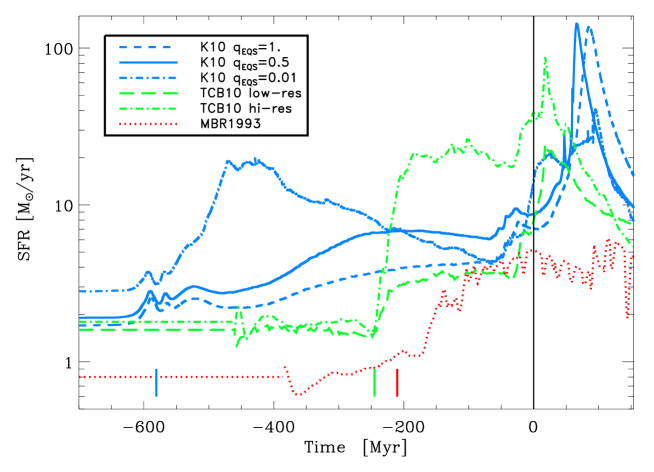
Figure 1.— Evolution of the star formation rates in different N-body+hydrodynamical simulations of the Antennae galaxies. Blue (Karl et al., 2010, K10, and this paper): strong feedback (dashed), intermediate feedback (solid), weak feedback (dot-dashed); green (Teyssier et al., 2010, TCB10): low-resolution (dotted), high-resolution (dot-dashed); and red dotted (Mihos et al., 1993, MBR93). The time of best match for each simulation is $t=0$ (at the vertical solid line). The time of first pericenter passage is indicated by colored vertical bars. Straight horizontal lines show the assumed constant star formation rates in the pre-interaction disks.

Fall et al. (2005) found that the age distribution of massive clusters in the Antennae galaxies can be approximated by a power law, $\chi(\tau)\equiv dN/d\tau\propto\tau^{\gamma}$ with $\gamma\approx-1$. The mass function of the clusters is also a power law, $\psi(M)\equiv dN/dM\propto M^{\beta}$ with $\beta\approx-2$ (Zhang & Fall, 1999). In fact, these results are parts of a broader finding; the bivariate distribution of masses and ages can be approximated by a product of power laws: $g(M,\tau)\propto\psi(M)\chi(\tau)\propto M^{\beta}\tau^{\gamma}$. This model has been derived from observations of massive clusters in the Antennae (roughly $M\gtrsim 10^{4}(\tau/10^{7}\mathrm{yr})^{0.7}\hbox{$\thinspace M_{\odot}$}$). The decomposition of $g(M,\tau)$ into a product of $\psi(M)$ and $\chi(\tau)$ implies that the (net) formation and disruption rates of the clusters are independent of their masses. The power-law model for $g(M,\tau)$ has been confirmed in subsequent observational studies of the Antennae clusters (Whitmore et al., 2007; Fall et al., 2009; Whitmore et al., 2010).

Similar results have now been obtained for the age distributions of clusters in about 20 other galaxies (although with smaller samples and thus larger uncertainties than for the Antennae galaxies). These include the Milky Way (Lada & Lada, 2003); the Large and Small Magellanic Clouds (Chandar et al., 2010a); NGC 1313, NGC 4395, NGC 5236 (M83), NGC 7793 (Mora et al., 2009; Chandar et al., 2010c); NGC 922 (Pellerin et al., 2010); NGC 3256 (Goddard et al., 2010); Arp 284 (Peterson et al., 2009); and nine nearby dwarf galaxies (Melena et al., 2009). The masses and ages of the clusters in these galaxies cover the ranges $10^{2}\hbox{$\thinspace M_{\odot}$}\lesssim M\lesssim 10^{6}\hbox{$\thinspace M_{\odot}$}$ and $\tau\lesssim 10^{9}$ yr. The galaxies themselves are also diverse, ranging from dwarf to giant, quiescent to interacting. Yet in all cases, the observed age distribution of the clusters can be represented by a power law,

$$dN/d\tau\propto\tau^{\gamma}\hskip 17.07182pt\mathrm{with}\hskip 17.07182pt-1.0\lesssim\gamma\lesssim-0.7,$$ (3)

where the exponents have uncertainties $\Delta\gamma\approx 0.1-0.2$. See Chandar et al. (2010b) for a more complete discussion of these results and the methods used to obtain them.

The stellar age distribution is known in detail only for three of the galaxies mentioned above: the Milky Way (Binney & Merrifield, 1998, and references therein), the LMC (Harris & Zaritsky, 2009), and the SMC (Harris & Zaritsky, 2004). In these cases, the star formation rate (SFR) has been constant to within a factor of 2 over the past $\sim 10^{9}$ yr, and we can be certain that the observed age distribution of the clusters primarily reflects their disruption history. From Equations (1) and (2) and the observed $dN/d\tau$ we obtain

$$f_{\rm surv} \propto \tau^{\delta}\hskip 17.07182pt\mathrm{with}\hskip 17.07182pt\delta\approx\gamma\approx-1.$$ (4)

Less is known about the star formation histories in the other galaxies. For some, the rate may have increased over the past $\sim 10^{9}$ yr, while for others, it may have decreased. However, if we assume that the average formation rate for the sample (which includes a fairly typical mix of galaxies) has been roughly constant, then Equations (1) and (2) and the observed $dN/d\tau$ again imply $f_{\rm surv}\;{{}^{\propto}_{\sim}}\;\tau^{\delta}$ with $\delta\approx\gamma\approx-1$. In fact, the average SFR over all galaxies has declined slightly in the past $\sim 10^{9}$ yr (Lilly et al., 1996; Madau et al., 1996). The alternative to this interpretation is that all 20 galaxies have the same rising star formation rate. However, the probability of this happening by chance is minuscule (roughly $(1/2)^{20}\approx 10^{-6}$ for equal numbers of rising and falling SFRs).

For the Antennae, we have another indication that the observed age distribution of the clusters reflects their disruption history rather than their formation history. Specifically, $dN/d\tau$ has approximately the same power-law shape in regions separated by $\sim 10$ kpc (Whitmore et al., 2007). This observation can be explained, in principle, either by disruption or by synchronized formation throughout the Antennae. Indeed, the spatial uniformity of $dN/d\tau$, combined with causality restrictions, places interesting constraints on possible temporal variations in the formation rate as follows (Fall et al., 2005, 2009; Whitmore et al., 2007). The timescale for variations in the formation rate, if these are driven by gravitational interactions, is the galactic orbital period, $\sim 10^{8}$ yr. Similarly, the communication time is $10^{8}$ yr or $10^{9}$ yr for a signal traveling a distance of 10 kpc at a velocity of 100 km s^-1 or 10 km s^-1, respectively, plausible values for pressure disturbances in the ISM. In either case, we expect the formation rate to vary relatively slowly, an expectation borne out nicely by the N-body+hydrodynamical simulations presented in the next section.

The mechanisms that disrupt clusters include the following: (1) removal of ISM by stellar feedback, $\tau\lesssim 10^{7}$ yr (Hills, 1980); (2) continued mass loss from intermediate- and low-mass stars, $10^{7}$ yr $\lesssim\tau\lesssim 10^{8}$ yr (Chernoff & Weinberg, 1990); (3) tidal disturbances by passing molecular clouds, $\tau\gtrsim 10^{8}$ yr (Spitzer, 1958); (4) stellar escape driven by internal two-body relaxation, $\tau\gtrsim 10^{9}$ yr (Spitzer, 1987). The timescales quoted above are highly approximate, and some of the mechanisms must in fact operate simultaneously. The interested reader is referred to Fall et al. (2009) and Fall et al. (2010) for further discussion of disruption mechanisms and how they relate to the mass and age distributions. In the present context, it is important to note that mechanisms (1), (2), and (4) have little or no dependence on the properties of the host galaxy. Only mechanism (3)—encounters with molecular clouds—is expected to have such a dependence, through the mean density of molecular gas. In practice, however, this is likely to make relatively little difference over much of the observed range of ages, and we therefore expect $f_{\rm surv}$ to be similar in different galaxies, consistent with the observations summarized above.

3. $N$-Body$+$Hydrodynamical Simulations

Interacting and merging galaxies like the Antennae generally show signs of enhanced star formation in the past few $\times 10^{8}{\rm\thinspace yr}$, along with more complex morphology and kinematics, compared with isolated disk galaxies. In this Section, we briefly present and analyze all published and two new simulations of the Antennae galaxies that make specific predictions for their star formation history. We do not claim that any of these simulations uniquely represents the real Antennae system. In particular, the spatial and temporal resolution in the simulations is much too low to model the ISM accurately on the scales of individual star clusters (Bekki et al., 2002; Kravtsov & Gnedin, 2005; Li et al., 2004). Nevertheless, these simulations provide us with a suite of plausible star formation histories for the Antennae. We adopt this approach because it would be difficult, if not impossible, to determine the stellar age distribution in the Antennae directly from observations.

Following the first N-body simulation of the Antennae Galaxies by TT72, several groups have improved the pure stellar dynamical models of the system (Barnes, 1988; Hibbard, 2003; Renaud et al., 2008, 2009). However, there are still only a few N-body+hydrodynamical simulations that predict star formation histories of the Antennae and, at the same time, provide a reasonable match to the gross morphology and kinematics of the system.

In the MBR93 simulation, the ISM is represented by discrete clouds that evolve by merging and fragmentation. Star formation is modeled using a Schmidt (1959) relation, $\dot{\rho}_{*}\propto\rho^{1.8}$, with an initial gas depletion timescale of $\approx 7{\rm\thinspace Gyr}$ (see Mihos et al., 1991, 1992, for details). The spatial and mass resolutions for the baryonic component (stars) are $x_{\mathrm{res}}=200{\rm\thinspace pc}$ and $m_{\mathrm{res}}=6.8\times 10^{6}\hbox{$\thinspace M_{\odot}$}$. The Antennae were modeled as two interacting identical disk galaxies (see Barnes, 1988) on an elliptical orbit with initial disk inclinations as in TT72. At the time of best match, after the first pericenter passage, the total SFR has increased by a factor of 6 with respect to the progenitor disks. Most of the star formation is concentrated in the two nuclei, with very little in the overlap region between them. Observations show, however, that most of the recent star and cluster formation takes place in the overlap region (e.g. Stanford et al., 1990; Mirabel et al., 1998; Zhang et al., 2001). We have reproduced the star formation history from Figure 10 of MBR93 in our Figure 1 (red dotted line). The intermittent nature of star formation in the MBR93 simulation, i.e. the rapid fluctuations in the overall SFR, is very likely a result of their particular discrete-cloud model of the ISM. To extend the simulated star formation histories to $\tau\gtrsim 10^{9}{\rm\thinspace yr}$, we assume a constant rate of star formation before the start of the simulations (i.e., the time at which the full N-body+hydrodynamical interactions are switched on) We adopt the same procedure for all the other simulations presented in the remainder of this section (see the constant horizontal lines in Figure 1).

Figure 2.— Star formation history from K10 with intermediate feedback, $q_{\rm eqs}=0.5$ (solid line, see also Figure 1). The coarse-grained, fluctuating age distribution of the spawned stellar particles from Figure 4 of K10 (dotted line/asterisks) is compared to the revised fine-grained age distribution used here (dashed line/diamonds). The age bins of the spawned particles have widths of $\Delta\log\tau=0.5$ as in K10.

Recently, K10 presented the first simulation of the Antennae that accounts for the extended star formation in the overlap region. For this study, the ISM was modeled by smoothed particle hydrodynamics (SPH; see Monaghan, 1992, for a review). Star formation again followed a Schmidt relation, with $\dot{\rho}_{*}\propto\rho^{3/2}$ and a characteristic gas depletion timescale of $t_{0}^{*}=8.4{\rm\thinspace Gyr}$ at the star formation threshold, $n_{\mathrm{crit}}=0.128{\rm\thinspace cm}^{-3}$. The K10 simulation also includes stellar feedback (Springel & Hernquist, 2003). The baryonic spatial and mass resolutions are $x_{res}=35{\rm\thinspace pc}$ and $m_{res}=7\times 10^{4}\hbox{$\thinspace M_{\odot}$}$. The progenitor galaxies were merged on a mildly elliptical orbit with disk orientations and a time of best match that resulted in better agreement with the observed large- and small-scale morphology and line-of-sight kinematics compared with previous Antennae simulations. In particular, the K10 simulation is the only published simulation that gives a reasonable spatial distribution of recent star formation activity, including the observed starburst in the overlap region (see also Kotarba et al., 2010).

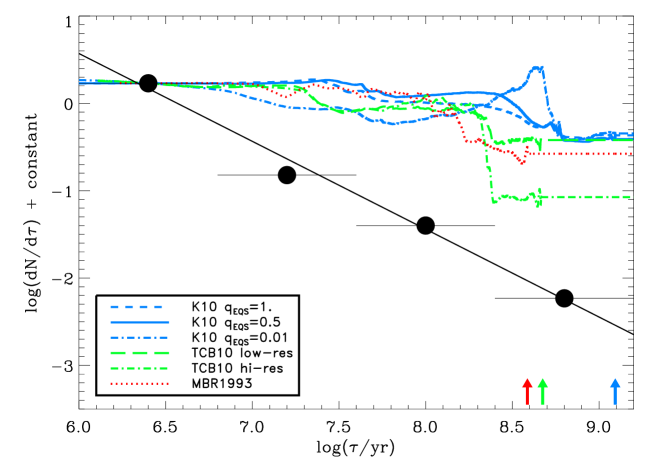
Figure 3.— Age distribution of star clusters derived from the star formation histories in the simulations shown in Figure 1 (without disruption). For comparison, we plot the observed age distribution of clusters with $M\geq 2\times 10^{5}\hbox{$\thinspace M_{\odot}$}$ in the Antennae (filled dots) from Fall et al. (2005). The diagonal line represents the power-law model, $dN/d\tau\propto\tau^{\gamma}$ with the best-fitting exponent $\gamma=-1.01\pm 0.03$. The simulated age distribution has been normalized to match the observed one at the midpoint of the youngest bin. The zeropoint of age is the time of best match in the simulations. The colored arrows indicate the starting times of the simulations.

K10 presented the stellar age distribution within the central $18{\rm\thinspace kpc}$ of the simulation at the time of best match (see their Figure 4). This distribution was based on the stellar particles spawned from the gas particles according to the Schmidt relation. The time sampling for the particle spawning adopted by K10, however, is too coarse for the detailed analysis presented here. This can be seen in Figure 2, where we compare the total star formation rate (solid line) with the age distribution of spawned particles (asterisks, 0.5 dex age bins). For ages older than a few $\times 10^{7}{\rm\thinspace yr}$, they are very similar. For younger ages, however, there are large fluctuations in the age distribution of spawned particles. In particular, this distribution is too high in the first bin and too low in the second bin. We emphasize that these fluctuations are artifacts caused by the coarse time-sampling of the spawning process; hence they have only a numerical, not a physical origin. To remedy this inconsistency, we have rerun the K10 simulation with a finer time sampling for the particle spawning and show the corresponding age distribution (0.5 dex binning) in Figure 2 (open diamonds). Now the age distribution closely follows the SFR even for young ages (as it should). In the following, we dispense entirely with the age distribution of spawned stellar particles and adopt the SFR computed directly from the Schmidt relation at each time step.

For the present study, we analyze the simulation presented in K10 together with two new simulations with the same orbital and other model parameters, but with different amounts of feedback. In these simulations, stellar feedback heats and pressurizes the ISM, thereby suppressing and regulating star formation (Springel & Hernquist, 2003). The energy input is controlled by a dimensionless parameter $q_{\mathrm{eqs}}$ that ranges from 0 (no feedback) to 1 (full feedback, see Springel et al., 2005, for details). In Figure 1, we show the star formation histories for the simulations with full feedback ($q_{\mathrm{eqs}}=1$, blue dashed), intermediate feedback ($q_{\mathrm{eqs}}=0.5$, blue solid) from K10, and very weak feedback ($q_{\mathrm{eqs}}=0.01$, blue dot-dashed). The SFR in the simulation with the strongest feedback ($q_{\mathrm{eqs}}=1$) increases only modestly after the first pericenter passage (vertical blue bar) and then again after the second pericenter passage, until it is 4 times higher at the time of best match than in the pre-interaction disk phase. Reducing the feedback ($q_{\mathrm{eqs}}=0.5$) results in a more efficient consumption of gas after the first close passage. At the time of best match, the SFR has increased only by a factor of 5. In the case of weak feedback ($q_{\mathrm{eqs}}=0.01$), the gas is consumed more rapidly in an early interaction phase, with a peak in star formation about $150{\rm\thinspace Myr}$ after the first pericenter passage. Thereafter, the SFR drops rapidly and then increases following the second pericenter passage to 5 times the initial value at the time of best match. Most of the star formation then occurs in the overlap region rather than in the two nuclei, in reasonable agreement with observations (Zhang et al., 2001; Wang et al., 2004; Brandl et al., 2009; Klaas et al., 2010).

TCB10 have recently presented a set of Antennae simulations based on the adaptive mesh refinement (AMR) grid code RAMSES (Teyssier, 2002) with the orbit of an earlier N-body simulation by Renaud et al. (2008, 2009). They model the ISM with a polytropic equation of state. Stellar feedback is not included, but thermal support is added on small scales to avoid artificial fragmentation. As in the simulations described above, star formation is modeled using a Schmidt relation in the form $\dot{\rho}_{*}\propto\rho^{3/2}$. TCB10 present low-resolution ($x_{res}=96{\rm\thinspace pc},m_{res}=10^{6}\hbox{$\thinspace M_{\odot}$}$) and high-resolution ($x_{res}=12{\rm\thinspace pc},m_{res}=4\times 10^{4}\hbox{$\thinspace M_{\odot}$}$) simulations in which the star formation thresholds are scaled (by almost two orders of magnitude higher in the latter case) to give similar SFRs in the progenitor disks. The gas depletion timescales at the star formation threshold are $16$ Gyr and $2$ Gyr, respectively, for the low- and high-resolution simulations. The star formation history of the TCB10 low-resolution simulation is shown by the green dashed line in Figure 1. As in the MBR93 simulation, the SFR increases moderately after the first pericenter passage (vertical green bar), by a factor of 4 at the time of best match. In the high-resolution simulation (green dot-dashed), the increase in the SFR after first pericenter passage is more dramatic, about 20 times higher at best match than in the progenitor disks. The star formation history, however, parallels the low-resolution case with an almost constant offset. In the K10 simulation with $q_{\mathrm{eqs}}=0.01$, a similar rise in the SFR after the first pericenter passage resulted from weak feedback. The high-resolution TCB10 simulation shows a more extended distribution of star forming sites, but these are not as smoothly connected as in the K10 simulations or as in the real Antennae (see Figure 1 in TCB10). Furthermore, the TCB10 simulations do not reproduce the observed starburst in the overlap region.

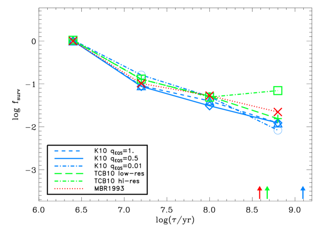
Figure 4.— Implied survival fraction of star clusters in the Antennae, $f_{\rm surv}\equiv(dN/d\tau)/(dN/d\tau)_{\rm form}$, plotted against age, with $dN/d\tau$ from Fall et al. (2005) and $(dN/d\tau)_{\rm form}$ from the simulations shown in Figure 1 (binned in the same way as the observations). The colored arrows indicate the starting times of the simulations.

The star formation histories in the simulations assembled here show a great deal of diversity, due to different orbits (merger timescales, orientations, etc) and/or different prescriptions for star formation and stellar feedback. The differences in the SFRs can be as much as an order of magnitude at a given evolutionary phase (e.g., the first pericenter passage). In all cases, the SFR is enhanced by the interaction relative to the quiescent disk phase, by factors of $4-20$ at the time of best match. However, most of this variation occurs early during the interaction, shortly after the first pericenter passage. In contrast, for $\tau\lesssim 2\times 10^{8}$ yr, the SFR varies remarkably slowly, by factors of 3 or less. This near-constancy of the recent SFR plays an important role in our interpretation of the observed age distribution of the star clusters in the Antennae galaxies.

4. Comparisons with Observations

We now compare the simulations with observations. The smooth curves in Figure 3 show the same simulated SFRs as Figure 1, but now plotted as $\log(dN/d\tau)$ against $\log(\tau/\mathrm{yr})$ with the zeropoint of age ($\tau=0$) taken to be the time of best match for each simulation. The data points in Figure 3 show the observed age distribution of massive clusters ($M\geq 2\times 10^{5}\hbox{$\thinspace M_{\odot}$}$) in the Antennae from Fall et al. (2005). The statistical uncertainties ($\sqrt{N}$) in each bin are $0.05$ – $0.06$ dex, about half the radius of the plotted symbols. The diagonal line in Figure 3 shows the power law that best fits the observations: $dN/d\tau\propto\tau^{\gamma}$ with $\gamma=-1.01\pm 0.03$. We have normalized the simulated and observed $dN/d\tau$ to a common value at the first data point. What is striking about Figure 3 is the divergence between the simulations and observations with increasing age, indicative of progressive disruption. At $\tau=10^{8}$ yr, for example, the observed age distribution has declined by a factor of 42, while the simulated formation rates have declined by factors of only $1.3$ – $2.5$, even in the midst of a dramatic collision between the galaxies. This illustrates the main conclusion of this paper: both the observed age distribution and simulated formation rates of clusters in the interacting Antennae galaxies resemble those in quiescent (non-interacting) galaxies. We demonstrate this conclusion more quantitatively in the remainder of this section.

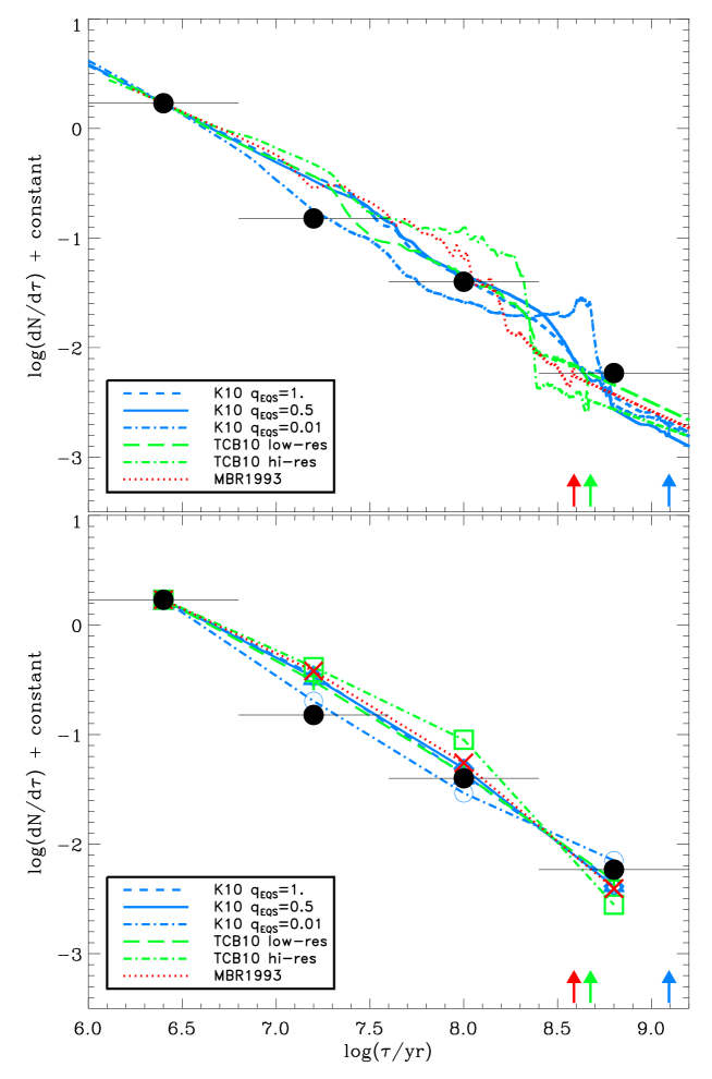
Figure 5.— Predicted age distribution of star clusters based on the simulated formation rates shown in Figure 1 and the power-law model for the survival fraction, $f_{\rm surv}\propto\tau^{\delta}$, with the best-fitting exponents listed in Table 1. For comparison, we show the observed age distribution (filled dots) from Fall et al. (2005). In the upper panel, the formation rates are unbinned; in the lower panel, they are binned in the same way as in the observations. The colored arrows indicate the starting times of the simulations.

The age distribution shown in Figure 3 is based on UBVIH$\alpha$ images taken with the Wide Field Planetary Camera 2 on HST. The masses and ages of the clusters were derived by comparing their luminosities and colors with stellar population models while correcting for interstellar extinction. The resulting age distribution is not sensitive to the particular choice of models or extinction curve. The data points plotted in Figure 3 pertain to a mass-limited sample with $M\geq 2\times 10^{5}\hbox{$\thinspace M_{\odot}$}$, which is essentially complete for ages up to $\tau\approx 10^{9}$ yr. The age distributions for samples limited at lower masses have the same power-law shape but do not extend to such large ages. In constructing the age distribution, relatively large bins were chosen ($\Delta\log\tau=0.8$) in order to smooth over small-scale features caused by the systematic errors that arise whenever masses and ages are estimated from multiband photometry. The most insidious of these is the artificial gap at $\tau\approx(1-2)\times 10^{7}$ yr resulting from stochastic variations in the colors of clusters caused by rapid evolution of a few bright red supergiant (RSG) stars. This so-called RSG gap, and other, less prominent features, affect every age distribution in this field — not just the one for the Antennae. The only practical way to minimize the corresponding systematic errors in the age distribution is to choose relatively large bins and to avoid centering any of them on the RSG gap. In the future, it may be possible to reduce the prominence of the RSG gap by augmenting the UBVIH$\alpha$ photometry with additional infrared photometry in several bands and/or spectra of large samples of clusters. The interested reader is referred to Fall et al. (2005) for a more complete discussion of the age distribution shown in Figure 3, including the many tests that were performed to determine its accuracy and robustness. Confirmation and further analysis can be found in the papers by Whitmore et al. (2007, 2010) and Fall et al. (2009).

The common normalization of $dN/d\tau$ at small $\tau$ in Figure 3 for both simulations and observations is required by our assumption that the formation rates of stars and clusters are linked together by Equation (2). In principle, we should equate $dN/d\tau$ and $(dN/d\tau)_{\rm form}$ at $\tau=0$, the only age at which we can be certain that no clusters have yet been disrupted, that they are all intact and observable, even if some of them are not gravitationally bound and will eventually disperse. This procedure implicitly fixes the constant of proportionality $c$ in Equation (2) between the formation rates of stars and observed clusters (in this case, those with $M\geq 2\times 10^{5}\hbox{$\thinspace M_{\odot}$}$). The dispersal time for unbound clusters is $\Delta\tau\sim 10^{7}$ yr ($\sim 10$ crossing times: see Fall et al., 2005 and Baumgardt & Kroupa, 2007). Thus, by matching $dN/d\tau$ and $(dN/d\tau)_{\rm form}$ at $\tau=2.5\times 10^{6}$ yr rather than $\tau=0$, we likely make only a small error, of order unity or much less. It would be a mistake to equate $dN/d\tau$ and $(dN/d\tau)_{\rm form}$ at $\tau>>10^{7}$ yr because in general this would cause a mismatch at young ages, the only part of the distribution for which disruption is guaranteed to be negligible.

We now explore several quantitative measures of the progressive disruption of clusters indicated by Figure 3. First, we divide the observed age distribution by the simulated formation rates (after binning in the same way) to obtain the implied survival fraction, $f_{\rm surv}\equiv(dN/d\tau)/(dN/d\tau)_{\rm form}$. This is plotted as a function of age in Figure 4. Evidently, $f_{\rm surv}$ declines monotonically up to $\tau=10^{8}$ yr for all simulations and up to $\tau=6\times 10^{8}$ yr for all but one simulation. The statistical significance of the decline in $f_{\rm surv}$ is 17–20 $\sigma$ from the first bin to the second, 5–9 $\sigma$ from the second bin to the third, and 8–16 $\sigma$ from the third bin to the fourth (again with one exception). Thus, a constant $f_{\rm surv}$ is definitely ruled out. A corollary of this result is that disruption continues at least up to $\tau\sim 10^{8}$ yr and possibly up to $\tau\sim 10^{9}$ yr. From Figure 4, it also appears that the survival fraction declines roughly as a power law of age.

Table 1Best-fit exponent $\delta$ in the power-law model of the survival fraction. 

Model	K10 $q=1.0$	$q=0.5$	$q=0.01$	TCB10 low-res	hi-res	MBR1993
$\delta$	$-0.86$	$-0.89$	$-0.88$	$-0.80$	$-0.62$	$-0.77$
Errors	$0.01$	$0.01$	$0.02$	$0.01$	$0.02$	$0.01$

We can make a more direct test of the power-law model for the survival fraction, $f_{\rm surv}\propto\tau^{\delta}$, by combining it with the formation rate $(dN/d\tau)_{\rm form}$ as in Equations (1) and (2). We then obtain the best-fit values of $\delta$ by minimizing $\chi^{2}$ between the predicted and observed age distributions $dN/d\tau$. The results of this comparison are listed in Table 1 and shown in Figure 5. In the upper panel of the figure, we plot the predicted $dN/d\tau$ without binning, while in the lower panel, we plot it with the same binning as the observations. The best-fit exponents lie in the range $-0.9\lesssim\delta\lesssim-0.6$ (with minor differences among the simulations). These are similar to, but slightly larger, than the exponent $\gamma=-1.0$ of the observed age distribution, because the simulated formation rates decline gradually with age (at least for $\tau\lesssim 2\times 10^{8}$ yr). We do not expect perfect agreement between any of the predicted and observed age distributions, because, as noted in Section 3, there is substantial diversity among the simulated formation histories themselves. Nevertheless, as Figure 5 shows, the predicted age distributions for all six simulations follow the same general, power-law trend as the observed age distribution. This is additional support for our conclusion that clusters in the Antennae are disrupted progressively over an extended period and in a manner similar to that in more quiescent galaxies such as the Milky Way and the Magellanic Clouds. Is is also gratifying to note that the simulation that best matches the age distribution (the K10 $q_{\rm EQS}=0.01$ simulation, dot-dashed blue line in Figure 5) also reproduces the extended star formation in the overlap region.

Bastian et al. (2009) reached a different conclusion: that the disruption of clusters ceases at $\tau\sim 10^{7}$ yr in the Antennae. Their analysis differs from ours in several respects. (1) Bastian et al. base their claim only on the MBR93 simulation. This simulation, however, fails to reproduce the observed spatial extent of recent star formation in the overlap region of the Antennae. (2) Bastian et al. equate the observed age distribution $dN/d\tau$ and the simulated formation rate $(dN/d\tau)_{\rm form}$ at relatively old ages, $\tau\sim 10^{8}$ yr. As we have emphasized above, $dN/d\tau$ and $(dN/d\tau)_{\rm form}$ must be matched near $\tau\approx 0$ in order to connect the formation rates of clusters and stars. (3) Bastian et al. have adopted an age distribution with a dip at $\tau=(1-3)\times 10^{7}$ yr and a secondary peak at $\tau=(3-10)\times 10^{7}$ yr from Whitmore et al. (2007). This is based on the same observations as the age distribution adopted here, but it has narrower bins ($\Delta\log\tau=0.5$), one of which, unfortunately, is centered right on the RSG gap. This dip-peak structure in the age distribution is not reproducible by any of the simulations considered here and we therefore regard it as an unphysical artifact associated with the RSG gap.

5. Conclusions

The main conclusion of this paper is that the star clusters in the interacting Antennae galaxies are disrupted in much the same way as those in other galaxies. In most if not all star-forming galaxies, including the Antennae, the observed age distribution of clusters can be approximated by a power law, $dN/d\tau\propto\tau^{\gamma}$, with an exponent in the range $-1.0\lesssim\gamma\lesssim-0.7$ (see Chandar et al., 2010b and Section 2 here). In general, this must reflect the combined formation and disruption histories of the clusters. However, variations in the formation rate are expected to be a minor influence because $dN/d\tau$ is so similar in different galaxies and declines by such a large factor, typically $\sim 10^{2}$, over a relatively small range of age, $\tau\lesssim 10^{8}$–$10^{9}$ yr (i.e., less than 10% of the lifetime of the galaxies). Indeed, in several well-studied galaxies (the Milky Way and the Magellanic Clouds), the SFR is known from observations to have been nearly constant for the past $\sim 10^{9}$ yr, compelling evidence that the decline in $dN/d\tau$ is mainly a consequence of disruption (Binney & Merrifield, 1998; Harris & Zaritsky, 2004, 2009; Chandar et al., 2010a).

The interpretation is less straightforward for the Antennae galaxies, since they are too far away to determine their star formation history from observations. Furthermore, it is natural to wonder whether the interaction could trigger enough recent formation to explain the shape of $dN/d\tau$ without disruption. Fall et al. (2005) argued that the formation rate would vary by factors of a few on the orbital timescale ($\sim 10^{8}$ yr), too gradually to account for most of the decline in $dN/d\tau$ (see also Whitmore et al., 2007 and Fall et al., 2009). The results presented here support this suggestion. We have assembled the star formation histories in all the available $N$-body$+$hydrodynamical simulations of the Antennae. These are based on different numerical methods, different orbits, and different prescriptions for star formation and stellar feedback. The treatment of small-scale processes is still approximate at best, due to the low resolution in the simulations compared to molecular clouds and clumps in the real ISM. The star formation rates differ greatly among the simulations, both in absolute level and in time dependence. Nevertheless, we find that they all vary slowly, by factors of only $1.3-2.5$ in the past $10^{8}$ yr. When we combine the formation rates in the simulations with a power-law model for the survival fraction of clusters, $f_{\rm surv}\propto\tau^{\delta}$, we find good agreement with the observed age distribution over the range $10^{6}$ yr $\lesssim\tau\lesssim 10^{9}$ yr for $-0.9\lesssim\delta\lesssim-0.6$. The similarity between $\delta$ and $\gamma$ indicates that $dN/d\tau$ is shaped mainly by the disruption of clusters rather than variations in their formation rate.

The only caveat to this conclusion stems from our assumption that the formation rates of clusters and stars are proportional to each other, i.e. $(dN/d\tau)_{\rm form}=c\cdot dN_{*}/d\tau$ with $c={\rm constant}$ (cf. Equation (2)). This is certainly true if most stars form in clusters, a hypothesis consistent with $\mathrm{H}{\alpha}$ observations of the Antennae (Fall et al., 2005). However, even if we were to abandon this assumption entirely, and allow $c$ to vary arbitrarily with $\tau$, a slightly modified version of the analysis presented above would then lead to the alternative result $c(\tau)\cdot f_{\rm surv}(\tau)\propto\tau^{\delta}$ with $-0.9\lesssim\delta\lesssim-0.6$. We would then be left with the problem of explaining why the product $c\cdot f_{\rm surv}$ but not $f_{\rm surv}$ in the Antennae happens to be the same as $f_{\rm surv}$ alone in other galaxies. The simplest interpretation — the one advocated here — is that the formation rates of clusters and stars do track each other and that the survival fractions and hence the disruption histories are similar in different galaxies, including the Antennae.

References

- Barnes (1988) Barnes, J. E. 1988, ApJ, 331, 699
- Bastian et al. (2009) Bastian, N., Trancho, G., Konstantopoulos, I. S., & Miller, B. W. 2009, ApJ, 701, 607
- Baumgardt & Kroupa (2007) Baumgardt, H. & Kroupa, P. 2007, MNRAS, 380, 1589
- Bekki et al. (2002) Bekki, K., Forbes, D. A., Beasley, M. A., & Couch, W. J. 2002, MNRAS, 335, 1176
- Binney & Merrifield (1998) Binney, J. & Merrifield, M. 1998, Galactic astronomy, ed. Binney, J. & Merrifield, M.
- Binney & Tremaine (2008) Binney, J. & Tremaine, S. 2008, Galactic Dynamics: Second Edition, ed. Binney, J. & Tremaine, S. (Princeton University Press)
- Bournaud et al. (2008) Bournaud, F., Duc, P.-A., & Emsellem, E. 2008, MNRAS, 389, L8
- Brandl et al. (2009) Brandl, B. R., et al. 2009, ApJ, 699, 1982
- Chandar et al. (2010a) Chandar, R., Fall, S. M., & Whitmore, B. C. 2010a, ApJ, 711, 1263
- Chandar et al. (2011) Chandar, R., Whitmore, B. C., Calzetti, D., Di Nino, D., Kennicutt, R. C., Regan, M., & Schinnerer, E. 2011, ApJ, 727, 88
- Chandar et al. (2010b) Chandar, R., Whitmore, B. C., & Fall, S. M. 2010b, ApJ, 713, 1343
- Chandar et al. (2010c) Chandar, R., et al. 2010c, ApJ, 719, 966
- Chernoff & Weinberg (1990) Chernoff, D. F. & Weinberg, M. D. 1990, ApJ, 351, 121
- Fall et al. (2005) Fall, S. M., Chandar, R., & Whitmore, B. C. 2005, ApJ, 631, L133
- Fall et al. (2009) —. 2009, ApJ, 704, 453
- Fall et al. (2010) Fall, S. M., Krumholz, M. R., & Matzner, C. D. 2010, ApJ, 710, L142
- Gieles et al. (2005) Gieles, M., Bastian, N., Lamers, H. J. G. L. M., & Mout, J. N. 2005, A&A, 441, 949
- Goddard et al. (2010) Goddard, Q. E., Bastian, N., & Kennicutt, R. C. 2010, MNRAS, 405, 857
- Harris & Zaritsky (2004) Harris, J. & Zaritsky, D. 2004, AJ, 127, 1531
- Harris & Zaritsky (2009) Harris, J. & Zaritsky, D. 2009, AJ, 138, 1243
- Hibbard (2003) Hibbard, J. E. 2003, in Bulletin of the American Astronomical Society, Vol. 35, Bulletin of the American Astronomical Society, 1413
- Hibbard et al. (2001) Hibbard, J. E., van der Hulst, J. M., Barnes, J. E., & Rich, R. M. 2001, AJ, 122, 2969
- Hills (1980) Hills, J. G. 1980, ApJ, 235, 986
- Karl et al. (2010) Karl, S. J., Naab, T., Johansson, P. H., Kotarba, H., Boily, C. M., Renaud, F., & Theis, C. 2010, ApJ, 715, L88 (K10)
- Kassin et al. (2003) Kassin, S. A., Frogel, J. A., Pogge, R. W., Tiede, G. P., & Sellgren, K. 2003, AJ, 126, 1276
- Klaas et al. (2010) Klaas, U., Nielbock, M., Haas, M., Krause, O., & Schreiber, J. 2010, A&A, 518, L44
- Kotarba et al. (2010) Kotarba, H., Karl, S. J., Naab, T., Johansson, P. H., Dolag, K., Lesch, H., & Stasyszyn, F. A. 2010, ApJ, 716, 1438
- Kravtsov & Gnedin (2005) Kravtsov, A. V. & Gnedin, O. Y. 2005, ApJ, 623, 650
- Lada & Lada (2003) Lada, C. J. & Lada, E. A. 2003, ARA&A, 41, 57
- Li et al. (2004) Li, Y., Mac Low, M., & Klessen, R. S. 2004, ApJ, 614, L29
- Lilly et al. (1996) Lilly, S. J., Le Fevre, O., Hammer, F., & Crampton, D. 1996, ApJ, 460, L1
- Madau et al. (1996) Madau, P., Ferguson, H. C., Dickinson, M. E., Giavalisco, M., Steidel, C. C., & Fruchter, A. 1996, MNRAS, 283, 1388
- McKee & Ostriker (2007) McKee, C. F. & Ostriker, E. C. 2007, ARA&A, 45, 565
- Melena et al. (2009) Melena, N. W., Elmegreen, B. G., Hunter, D. A., & Zernow, L. 2009, AJ, 138, 1203
- Mihos et al. (1993) Mihos, J. C., Bothun, G. D., & Richstone, D. O. 1993, ApJ, 418, 82 (MBR93)
- Mihos et al. (1991) Mihos, J. C., Richstone, D. O., & Bothun, G. D. 1991, ApJ, 377, 72
- Mihos et al. (1992) —. 1992, ApJ, 400, 153
- Mirabel et al. (1998) Mirabel, I. F., Vigroux, L., Charmandaris, V., Sauvage, M., Gallais, P., Tran, D., Cesarsky, C., Madden, S. C., & Duc, P.-A. 1998, A&A, 333, L1
- Monaghan (1992) Monaghan, J. J. 1992, ARA&A, 30, 543
- Mora et al. (2009) Mora, M. D., Larsen, S. S., Kissler-Patig, M., Brodie, J. P., & Richtler, T. 2009, A&A, 501, 949
- Pellerin et al. (2010) Pellerin, A., Meurer, G. R., Bekki, K., Elmegreen, D. M., Wong, O. I., & Knezek, P. M. 2010, AJ, 139, 1369
- Peterson et al. (2009) Peterson, B. W., Struck, C., Smith, B. J., & Hancock, M. 2009, MNRAS, 400, 1208
- Renaud et al. (2008) Renaud, F., Boily, C. M., Fleck, J., Naab, T., & Theis, C. 2008, MNRAS, 391, L98
- Renaud et al. (2009) Renaud, F., Boily, C. M., Naab, T., & Theis, C. 2009, ApJ, 706, 67
- Schmidt (1959) Schmidt, M. 1959, ApJ, 129, 243
- Schweizer et al. (2008) Schweizer, F., et al. 2008, AJ, 136, 1482
- Spitzer (1987) Spitzer, L. 1987, Dynamical evolution of globular clusters, ed. Spitzer, L.
- Spitzer (1958) Spitzer, Jr., L. 1958, ApJ, 127, 17
- Springel et al. (2005) Springel, V., Di Matteo, T., & Hernquist, L. 2005, MNRAS, 361, 776
- Springel & Hernquist (2003) Springel, V. & Hernquist, L. 2003, MNRAS, 339, 289
- Stanford et al. (1990) Stanford, S. A., Sargent, A. I., Sanders, D. B., & Scoville, N. Z. 1990, ApJ, 349, 492
- Teyssier (2002) Teyssier, R. 2002, A&A, 385, 337
- Teyssier et al. (2010) Teyssier, R., Chapon, D., & Bournaud, F. 2010, ApJ, 720, L149 (TCB10)
- Toomre & Toomre (1972) Toomre, A. & Toomre, J. 1972, ApJ, 178, 623 (TT72)
- Wang et al. (2004) Wang, Z., Fazio, G. G., Ashby, M. L. N., Huang, J.-S., Pahre, M. A., Smith, H. A., Willner, S. P., Forrest, W. J., Pipher, J. L., & Surace, J. A. 2004, ApJS, 154, 193
- Whitmore et al. (2007) Whitmore, B. C., Chandar, R., & Fall, S. M. 2007, AJ, 133, 1067
- Whitmore et al. (2010) Whitmore, B. C., Chandar, R., Schweizer, F., Rothberg, B., Leitherer, C., Rieke, M., Rieke, G., Blair, W. P., Mengel, S., & Alonso-Herrero, A. 2010, AJ, 140, 75
- Zezas et al. (2006) Zezas, A., Fabbiano, G., Baldi, A., Schweizer, F., King, A. R., Ponman, T. J., & Rots, A. H. 2006, ApJS, 166, 211
- Zhang & Fall (1999) Zhang, Q. & Fall, S. M. 1999, ApJ, 527, L81
- Zhang et al. (2001) Zhang, Q., Fall, S. M., & Whitmore, B. C. 2001, ApJ, 561, 727