From SO/Sp instantons to W-algebra blocks

Abstract:

We study instanton partition functions for ${\cal N}=2$ superconformal $Sp(1)$ and $SO(4)$ gauge theories. We find that they agree with the corresponding $U(2)$ instanton partitions functions only after a non-trivial mapping of the microscopic gauge couplings, since the instanton counting involves different renormalization schemes. Geometrically, this mapping relates the Gaiotto curves of the different realizations as double coverings. We then formulate an AGT-type correspondence between $Sp(1)/SO(4)$ instanton partition functions and chiral blocks with an underlying ${\cal W}(2,2)$-algebra symmetry. This form of the correspondence eliminates the need to divide out extra $U(1)$ factors. Finally, to check this correspondence for linear quivers, we compute expressions for the $Sp(1)\times SO(4)$ half-bifundamental.

1 Introduction

Over the last year a substantially deeper understanding has been obtained of S-duality in four-dimensional supersymmetric gauge theories and of the relation to two-dimensional geometry and conformal field theory (see for instance [1, 2, 3, 4, 5]).

The simplest example of S-duality appears in ${\cal N}=4$ supersymmetric gauge theory. Such a gauge theory is characterized purely by the choice of a gauge group $G$ and a value for the complexified gauge coupling $\tau$. The theory has long been known to be invariant under $SL(2,\mathbb{Z})$ transformations of the coupling $\tau$, which can be geometrically realized as Möbius transformations of a two-torus $T^{2}$ with complex structure parameter $\tau$.

S-duality in ${\cal N}=4$ gauge theory translates into modular properties of its instanton partition function. In particular, the ${\cal N}=4$ instanton partition function for gauge group $G$ is argued to be a character for the affine Lie algebra $\hat{\mathfrak{g}}$ [6, 7, 8]. This character also appears as the partition function of a two-dimensional conformal field theory with current algebra $\hat{\mathfrak{g}}$ on the two-torus $T^{2}$. This implies a close relation between ${\cal N}=4$ gauge theory and two-dimensional conformal field theory on $T^{2}$. Such a connection is most naturally understood by embedding the ${\cal N}=4$ gauge theory on a set of M5-branes wrapping the four-manifold times the two-torus $T^{2}$ [9, 10].

Supersymmetric ${\cal N}=2$ gauge theories are much richer than their ${\cal N}=4$ counterparts. Not only can different kinds of matter multiplets be added to the theory, but even for conformal theories the gauge coupling receives a finite renormalization. In the low-energy limit the gauge theory is characterized by a two-dimensional Seiberg-Witten curve, whose geometry captures the prepotential of the gauge theory as well as the masses of BPS particles [11, 12]. Using a brane realization of the ${\cal N}=2$ gauge theory in string or M-theory, the Seiberg-Witten curve naturally comes about as a branched covering over yet another two-dimensional curve [13]. We will refer to this base curve as the Gaiotto curve (or G-curve). Mathematically, the ${\cal N}=2$ geometry is encoded in a ramified Hitchin system.

It was realized recently that it is important to not forget about the additional information contained in the covering structure of the Seiberg-Witten curve. In particular, it is conjectured that the complex moduli space of the Gaiotto curve is the parameter space of the exactly marginal couplings of the superconformal ${\cal N}=2$ gauge theory [1]. Analogous to the ${\cal N}=4$ example, this suggests good transformation properties of the ${\cal N}=2$ partition function under mapping class group transformation of the Gaiotto curve. Furthermore, it hints at an extension of the relation between four-dimensional gauge theories and two-dimensional conformal field theories to ${\cal N}=2$ supersymmetric gauge theories.

Indeed, such a relation between ${\cal N}=2$ gauge theory and two-dimensional conformal field theory has been found [2], and is referred to as the AGT correspondence. In particular, an equivalence was discovered between $U(2)$ instanton partition functions and Virasoro conformal blocks. This was extended to asymptotically free theories [14], to $U(N)$ theories [15] and to inclusion of surface operators (see amongst others [16, 17, 18, 19, 20, 21, 22, 23, 24]).

Nonetheless, a few important open questions remain, such as a good understanding through the M5-brane picture, the extension to generalized quivers and general gauge groups, and a better explanation of the spurious $U(1)$ factor which appears in the AGT correspondence. In this paper we start by tackling the last question, and gradually gain more insight in the correspondence between four-dimensional ${\cal N}=2$ gauge theories and two-dimensional conformal field theory.

In [2] it was found that after a suitable identification of parameters the conformal block agrees with an instanton partition function for gauge group $U(2)$, whose Coulomb branch parameters are specialized to $SU(2)$ values, up to a spurious factor. This spurious factor closely resembles the partition function of a $U(1)$ gauge theory. The interpretation given was therefore that the partition function of $U(2)$ factorizes into an $SU(2)$ part which corresponds to the conformal block, and a $U(1)$ part which decouples [20].

There is no direct way to compute instanton partition functions for $SU(N)$ theories. What one does instead is to consider the construction for $U(N)$ and then impose tracelessness of the Coulomb branch parameters in the end. From this point of view one might expect the appearance of an additional $U(1)$ factor, which corresponds to the overall $U(1)$ that somehow decouples.

For $SU(2)$ however there is a direct computation of the partition function, which uses the fact that $SU(2)=Sp(1)$. A similar situation arises for $SO(4)\cong SU(2)\times SU(2)$. In both cases we can thus obtain the partition function either by a direct computation, or by computing the corresponding $U(2)$ partition functions and splitting off $U(1)$ factors. The computation of the $Sp(1)$ and $SO(4)$ partition functions are technically more difficult than the $U(2)$ case. We describe a procedure for the computation in appendix B, which we use to compute the $Sp(1)$ result up to instanton number $k=6$. Somewhat surprisingly, however, we find that for the conformal version of the theories with hypermultiplets, the computations naively look completely different. In particular, it does not seem possible to split off a $U(1)$ factor to make them agree.

We argue in this article that this difference is due to the fact that in the two computations one implicitly chooses a different renormalization scheme. More precisely, from our computation of the instanton contributions to the prepotential of these theories we can read off the relation between the microscopic gauge couplings $q$ in the UV and the gauge couplings $\tau$ in the IR. Once we express the instanton partition functions in terms of infrared variables, it turns out that both expressions agree. The different choices of renormalization schemes therefore correspond to different parametrizations of the moduli space of the theory in terms of microscopic gauge couplings. In the case at hand we find in fact a very simple relation between the two parametrizations. We also the discuss in detail the situation for $SO(4)$ as opposed to $U(2)\times U(2)$, which leads to similar results, and we argue that we can expect such a relation for any two different appearances of the same physical gauge theory.

The fact that we find such simple relations between the UV gauge couplings implies that there should be a geometric interpretation. In section 3 we thus turn to a string theory embedding of those gauge theories. More precisely, we discuss the underlying Gaiotto curve of the theories, whose complex structure moduli are given by the UV couplings $q$. From a string theory point of view $U(2)$ and $Sp(1)$ naturally lead to two different G-curves. In fact we show that the $U(2)$ curve is the double cover of the $Sp(1)$ curve, and their complex structure moduli are related in exactly the way we obtained from the instanton computation. Again, the situation for $SO(4)$ and $U(2)\times U(2)$ is completely analogous.

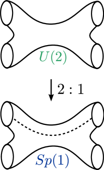
Figure 1: The Gaiotto curve of the $U(2)$ gauge theory coupled to 4 hypers as a double cover over the Gaiotto curve of the $Sp(1)$ theory. The dotted line is a branch cut.

Finding a geometric interpretation of the relation between those theories leads us to the second focus of this article. We want to find an AGT-like relation for more general gauge groups, like $Sp(1)$ and $SO(4)$, i.e. we want to find a configuration of a conformal field theory whose chiral block agrees directly with the $Sp(1)$ or $SO(4)$ partition function.

For general reasons we expect the symmetry of the CFT to be related to the gauge group $G$. More precisely, we argue that the Lie algebra structure of the Hitchin system is reflected in the ${\cal W}$-algebra that describes the symmetry of the CFT, in such a way that the generators of the ${\cal W}$-algebra are determined by the Casimirs of the Lie algebra $\mathfrak{g}$. In section 4, we find configurations whose ${\cal W}$-blocks agree with the $Sp(1)$ and $SO(4)$ partition functions, which we check for the first few orders by explicit computation. As expected, no additional $U(1)$ factor appears for this kind of AGT-like relation.

We also find a natural interpretation for the double cover map found geometrically from the conformal field theory side: The CFT configurations we consider involve $\mathbb{Z}_{2}$-twist fields and lines. The standard method to compute such correlators is to map them to a double cover, which gives a configuration without any twist fields that is straightforward to compute. For $Sp(1)$ and $SO(4)$ it turns out that the configuration on the cover is exactly the Virasoro conformal block on the four punctured sphere and the two punctured torus, respectively, which were found in [2] to correspond to the conformal $U(2)$ and $U(2)\times U(2)$ gauge theories.

Lastly, in section 5 we then formulate what the correspondence will look like for linear quivers. That is, quivers with alternating $Sp/SO$ gauge groups coupled by bifundamental half-hypermultiplets. We write down the instanton partition function for these bifundamental fields and check that the result indeed agrees with the chiral block of the corresponding CFT configuration.

Additional information can be found in the appendices. In appendix A we review the Nekrasov method of instanton counting in detail and give the derivations of the formulae that we use in the main body of the paper. In appendix B, we give a detailed explanation of how we evaluate the (refined) instanton partition function for $Sp/SO$ theories up to order 6 in the instanton parameter. Finally in appendix C, we compare $SU(2)$ Seiberg-Witten curves from different perspectives.

Notation: Let us explain our conventions for naming gauge groups to avoid confusion. We will say $Sp(1)$ if we refer to using the $Sp(1)$ renormalization scheme, and $U(2)$ if we refer to the $U(2)$ renormalization scheme with Coulomb branch parameters specialized to $a=a_{1}=-a_{2}$.

2 Instanton counting for $Sp/SO$ versus $U$ gauge groups

In this section we explore ${\cal N}=2$ instanton partition functions for symplectic and orthogonal gauge groups. We compare this to instanton counting for unitary gauge groups in cases when there exist both a unitary and a symplectic/orthogonal way of counting instantons. Examples of such specific instances are $Sp(1)$ versus $U(2)$, and $SO(4)$ versus $U(2)\times U(2)$. The two ways of counting instantons are not obviously the same, since they are based on a different realization of the instanton moduli space. Nonetheless, the two ways should give physically equivalent results in order for instanton counting for general gauge groups to make sense.

In this section we compare instanton partition functions for such specific instances. It turns out that the instanton partition functions for conformal gauge theories with these gauge groups are not equal on the nose. More precisely, they cannot even be related by a factor that is independent of the gauge theory moduli. We resolve this apparent disagreement by carefully examining the dependence of the instanton partition function on the microscopic versus physical gauge couplings. We find that instanton counting for different appearances of a gauge group are in general related by the choice of an inequivalent renormalization scheme.

One of the examples that we study in detail is $Sp(1)$ versus $U(2)$ instanton counting. We perform the instanton computations directly for $Sp(1)$, and then compare the results to the much better understood $U(2)$ instanton partition functions. Our motivation for studying this particular example is to gain a better understanding of the spurious factors that appear in the relation between $U(2)$ instanton partition functions and Virasoro blocks in the AGT correspondence. We will return to this issue in section 4, which also contains a summary of the AGT correspondence.

2.1 Instanton counting

At low energies the four-dimensional ${\cal N}=2$ gauge theory is governed by the prepotential ${\cal F}_{0}$, which determines the metric on the Coulomb branch of the gauge theory. Classically, the metric on the Coulomb branch is flat and the prepotential

$${\cal F}_{0}^{\rm clas}=2\pi i\,\tau_{UV}\,\vec{a}\cdot\vec{a},$$ (1)

is proportional to the microscopic coupling constant $\tau_{\rm UV}$. At the quantum level the prepotential receives both one-loop and non-perturbative instanton corrections, which give corrections to the metric on the Coulomb moduli space. The instanton corrections to the prepotential can be computed as equivariant integrals over the instanton moduli space [25]. Let us briefly sketch how this comes about. We refer to appendix A for a detailed discussion.

Instantons on $\mathbb{R}^{4}$ are solutions of the self-dual instanton equation

$$F^{+}_{A}=0.$$ (2)

The instanton moduli space ${\cal M}^{G}$ parametrizes these solutions up to gauge transformations that leave the fiber at infinity fixed. The components ${\cal M}^{G}_{k}$ of the instanton moduli space are labeled by the topological instanton number $k=1/8\pi^{2}\int F_{A}\wedge F_{A}$. The instanton corrections to the prepotential for the pure ${\cal N}=2$ gauge theory are captured by the instanton partition function

$$Z^{\rm inst}=\sum_{k}q^{k}\oint_{{\cal M}^{G}_{k}}1,$$ (3)

where $\oint 1$ formally computes the volume of the moduli space. The parameter $q$ can be considered as a formal parameter which counts the number of instantons. Physically, it is identified with a power $q=\Lambda^{b_{0}}$ of the dynamically generated scale $\Lambda$, when the gauge theory is asymptotically free. The power $b_{0}$ is determined by the one-loop $\beta$-function. It is identified with an exponent $q=\exp(2\pi i\tau_{\rm UV})$ of the microscopic coupling $\tau_{\rm UV}$ when the beta-function of the gauge theory vanishes.

If we introduce hypermultiplets to the pure ${\cal N}=2$ gauge theory, the instanton correction to the prepotential are instead determined by solutions of the monopole equations

$$F_{A,\mu\nu}^{+}+\frac{i}{2}\ \overline{q}_{\alpha}\Gamma^{\hskip 9.95845pt\alpha}_{\mu\nu\hskip 5.69054pt\beta}q^{\beta} =0,$$ (4)

$$\sum_{\mu}\Gamma^{\mu}_{\dot{\alpha}\alpha}D_{A,\mu}q^{\alpha} =0.$$

In these equations $\Gamma^{\mu}$ are the Clifford matrices and $\sum_{\mu}\Gamma^{\mu}D_{A,\mu}$ is the Dirac operator in the instanton background for the gauge field $A$. Although there are no positive chirality solutions to the Dirac equation, the vector space of negative chirality solutions is $k$-dimensional. Because this vector space depends on the gauge background $A$, it is useful to view it as a $k$-dimensional vector bundle over the instanton moduli space ${\cal M}^{G}_{k}$. We will call this vector bundle ${\cal V}$. More precisely, since the solutions to the Dirac equations are naturally twisted by the half-canonical line bundle ${\cal L}$ over $\mathbb{R}^{4}$ we will denote it by ${\cal V}\otimes{\cal L}$.

Instanton corrections to the ${\cal N}=2$ gauge theory, with $N_{f}$ hypermultiplets in the fundamental representation of the gauge group, are computed by the instanton partition function

$$Z^{\rm inst}=\sum_{k}q^{k}\oint_{{\cal M}^{G}_{k}}e({\cal V}\otimes{\cal L}\otimes M),$$ (5)

which is the integral of the Euler class of the vector bundle ${\cal V}\otimes{\cal L}$ of solutions to the Dirac equation over the moduli space ${\cal M}^{G}_{k}$. The flavor vector space $M=\mathbb{C}^{N_{f}}$ encodes the number of hypermultiplets in the gauge theory.

A difficulty in the evaluation of the instanton partition functions (3) and (5) is that the instanton moduli space ${\cal M}^{G}_{k}$ both suffers from an UV and an IR non-compactness. Instantons can become arbitrary small, as well as move away to infinity in $\mathbb{R}^{4}$. The IR non-compactness can be solved by introducing the $\Omega$-background, which refers to the action of the torus

$$\mathbf{T}^{2}_{\epsilon_{1},\epsilon_{2}}=U(1)_{\epsilon_{1}}\times U(1)_{\epsilon_{2}}$$ (6)

on $\mathbb{R}^{4}=\mathbb{C}\oplus\mathbb{C}$ by a rotation $(z_{1},z_{2})\mapsto(e^{i\epsilon_{1}}z_{1},e^{i\epsilon_{2}}z_{2})$ around the origin with parameters $\epsilon_{1},\epsilon_{2}\in\mathbb{C}$. If we localize the instanton partition function equivariantly with respect to the $\mathbf{T}^{2}_{\epsilon_{1},\epsilon_{2}}$-action, only instantons at the fixed origin will contribute, so that we can ignore the instantons that run off to infinity. The UV non-compactness can be cured for gauge group $U(N)$ by turning on an FI parameter. For $Sp$ and $SO$ gauge groups it is shown in [26] how to evaluate the instanton integrals, while implicitly curing the UV non-compactness of the instanton moduli space. Note that this effectively means that we have introduced a renormalization scheme.

Apart from the torus $\mathbf{T}^{2}_{\epsilon_{1},\epsilon_{2}}$ there are a few other groups that act on the instanton moduli space ${\cal M}^{G}_{k}$. Their actions can be understood best from the famous ADHM construction of the instanton moduli space [27]. This construction gives the moduli space as the quotient of the solutions of the ADHM equations by the so-called dual group $G^{D}_{k}$ with Cartan torus $\mathbf{T}^{k}_{\phi_{i}}$ whose weights we will call $\phi_{i}$. There is a also natural action of the Cartan torus $\mathbf{T}^{N}_{\vec{a}}$ of the framing group $G$ on the ADHM solution space, whose weights are given by the Coulomb branch parameters $\vec{a}$. Last, if the theory contains hypermultiplets, there is furthermore an action of the Cartan $\mathbf{T}^{N_{f}}_{\vec{m}}$ of the flavor symmetry group acting on $M$, whose weights correspond to the masses $\vec{m}$ of the hypers.

In total, we want to compute the partition function equivariantly with respect to the torus

$$\mathbf{T}=\mathbf{T}^{2}_{\epsilon_{1},\epsilon_{2}}\times\mathbf{T}^{N}_{\vec{a}}\times\mathbf{T}^{k}_{\phi_{i}}\times\mathbf{T}^{N_{f}}_{\vec{m}},$$ (7)

which comes down to computing the equivariant character of the action of those four tori. This results in a rational function $\mathbf{z}^{k}(\phi_{i},\vec{a},\vec{m},\epsilon_{1},\epsilon_{2})$ of the weights. From the construction of the Dirac bundle it is clear that $\textbf{z}^{k}$ factorizes if there are multiple hypers. Finally, we need to take into account the ADHM quotient. This we do by integrating over the dual group $G^{D}_{k}$. In total the instanton partition function is given by the integral

$$Z^{\rm inst}_{k}=\int\prod_{i}d\phi_{i}\,\mathbf{z}^{k}_{\textrm{gauge}}(\phi_{i},\vec{a},\epsilon_{1},\epsilon_{2})\,\mathbf{z}^{k}_{\textrm{matter}}(\phi_{i},\vec{a},\vec{m},\epsilon_{1},\epsilon_{2}),$$ (8)

where all the ${\cal N}=2$ multiplets in the gauge theory give a separate contribution. The instanton partition function of in principle any ${\cal N}=2$ gauge theory with a Lagrangian prescription can be computed in this way. Explicit expressions can be found in appendix A.

The integrand of (8) will have poles on the real axis. To cure this we will introduce small positive imaginary parts for the equivariance parameters. At least for asymptotically free theories we can then convert (8) into a contour integral, so that the problem reduces to enumerating poles and evaluating their residues. For $U(N)$ theory the poles are labeled by $N$ Young diagrams with in total $k$ boxes [25, 28, 29]: one way of phrasing this is that the $U(N)$ instanton splits into $N$ non-commutative $U(1)$ instantons.

For the $Sp(N)$ or $SO(N)$ theory it is not that simple to enumerate the poles of the contour integrals. Furthermore, not only the fixed points of the gauge multiplet are more complicated, but (in contrast to the $U(N)$ theory) also matter multiplets contribute additional poles. As an example, in appendix B we devise a technique to enumerate all the poles for an $Sp(N)$ gauge multiplet. Each pole can still be expressed as a generalized diagram with signs, but the prescription is much more involved than in the $U(N)$ case.

The instanton partition function $Z^{\rm inst}$ in the $\Omega$-background obviously depends on the equivariant parameters $\epsilon_{1}$ and $\epsilon_{2}$. In fact, it is rather easy to see that the series expansion of $\log(Z^{\rm inst})$ starts out with a term proportional to $\frac{1}{\epsilon_{1}\epsilon_{2}},$ which is the regularized volume of the $\Omega$-background. Even better, $Z^{\rm inst}$ has a series expansion

$$Z^{\rm inst}=\exp{\cal F}^{\rm inst}=\exp\left(\sum_{g=0}^{\infty}\hbar^{2g-2}{\cal F}^{\rm inst}_{g}(\beta)\right),$$ (9)

in terms of the parameter $\hbar^{2}=-\epsilon_{1}\epsilon_{2}$ and $\beta=-\frac{\epsilon_{1}}{\epsilon_{2}}$. We call the exponent of the instanton partition function the instanton free energy ${\cal F}^{\rm inst}$. As our notation suggests, we recover the non-perturbative instanton contribution to the prepotential ${\cal F}_{0}$ from the leading contribution of the exponent when $\hbar\to 0$. This has been showed in [33, 28, 34]. Let us emphasize that the prepotential ${\cal F}_{0}$ does not depend on the parameter $\beta$. The higher genus free energies ${\cal F}_{g\geq 1}(\beta)$ compute gravitational couplings to the ${\cal N}=2$ gauge theory, and play an important role in for example (refined) topological string theory.

To recover the full prepotential, we need to add classical and 1-loop contributions to the instanton partition function. We call the complete partition function

$$Z^{\rm Nek}=Z^{\rm clas}Z^{\rm 1-loop}Z^{\rm inst}$$ (10)

the Nekrasov partition function.

2.2 Infrared versus ultraviolet

Let us now turn to the goal of this section, which is comparing Nekrasov partition functions for gauge theories whose gauge group can be represented in two ways, possibly differing by a $U(1)$ factor. Think for instance of $Sp(1)$ versus $U(2)$ or $SO(4)$ versus $U(2)\times U(2)$. With a view on the AGT correspondence we are particularly keen on comparing $Sp(1)$ and $U(2)$ partition functions for conformally invariant theories. Naively, we would expect that the difference simply reproduces the “$U(1)$ factor”. As we report in subsection 2.3, however, the Nekrasov partition functions of the $Sp(1)$ and $U(2)$ gauge theory coupled to four hypermultiplets are not at all related in such a simple way.

To find a resolution of this disagreement, we should keep in mind the difference between infrared and ultraviolet quantities. Whereas the Nekrasov partition function $Z^{\rm Nek}(q)$ computes low-energy quantities, such as the prepotential ${\cal F}_{0}$, it is defined in terms of a series expansion in the exponentiated microscopic gauge coupling $q=\exp(2\pi i\tau_{UV})$. The gauge coupling $\tau_{UV}$, however, is sensitive to the choice of the renormalization scheme and therefore cannot be assigned a physical (low-energy) meaning. As we have pointed out in section 2.1, the renormalization schemes in the two instanton computations indeed differ. This means in particular that we should not identify the microscopic gauge couplings for the $U(2)$ and the $Sp(1)$ gauge theory. Instead, we should only expect to find agreement between the $Sp(1)$ and $U(2)$ Nekrasov partition functions when we express them in terms of physical low energy variables.

Figure 2: The period matrix $\tau_{\rm IR,ij}$ of the Seiberg-Witten curve is equal to the second derivative $\partial_{a_{i}}\partial_{a_{j}}{\cal F}_{0}$ of the prepotential with respect to the Coulomb parameter $a$. The imaginary part of $\tau_{\rm IR}$ determines the metric on the Coulomb branch.

What are such low energy variables? Recall that in the low energy limit of the ${\cal N}=2$ gauge theory the Coulomb branch opens up, which is classically parametrized by the Casimirs of the gauge group. The prepotential ${\cal F}_{0}$ of the ${\cal N}=2$ gauge theory determines the corrections to the metric on the Coulomb branch, whose imaginary part in turn prescribes the period matrix $\tau_{\rm IR}$ of the so-called Seiberg-Witten curve [11, 12]. As the Seiberg-Witten curve changes along with the Coulomb moduli $a$, its Jacobian defines a torus-fibration over the Coulomb branch (see Figure 2). Whereas for asymptotically free gauge theories the Seiberg-Witten curve depends on the dynamically generated scale $\Lambda$, for conformally invariant gauge theories the Seiberg-Witten curve is dependent on the value of the microscopic gauge couplings $\tau_{UV}$. Conformally invariant theories are characterized by a moduli space for the UV gauge couplings, from each element of which a Coulomb moduli space emanates in the low energy limit.

Since the Seiberg-Witten curve determines the masses of BPS particles in the low-energy limit of the ${\cal N}=2$ gauge theory, its period matrix $\tau_{\rm IR}$ is a physical quantity that should be independent of the chosen renormalization scheme. In contrast, the microscopic gauge couplings $\tau_{\rm UV}$ are characteristics of the chosen renormalization scheme.

To be more concrete, we can use the prepotential ${\cal F}_{0}$ computed from the Nekrasov partition function to find the relation between $\tau_{\rm IR}$ and $\tau_{\rm UV}$ by

$$2\pi i\tau_{\rm IR}=\frac{1}{2}\partial_{a}^{2}{\cal F}_{0}(\tau_{\rm UV},a)=\frac{1}{2}\partial_{a}^{2}({\cal F}_{0,\rm pert}+{\cal F}_{0,\rm inst})(\tau_{\rm UV},a)\,.$$ (11)

Here ${\cal F}_{0,\rm pert}$ contains the classical as well as 1-loop contribution to the prepotential, which for instance can be found in [35]. In particular, if two prepotentials that are computed using two different schemes differ by an $a$-dependent term, then the corresponding relations between $\tau_{\rm IR}$ and $\tau_{\rm UV}$ differ as well. If we invert the relation (11), and express both Nekrasov partition functions $Z^{\rm Nek}$ in terms of the period matrix $\tau_{\rm IR}$, we expect that they should agree up to a possible spurious factor that doesn’t depend on the Coulomb parameters. This says that the two ways of instanton counting correspond to two distinct renormalization schemes.

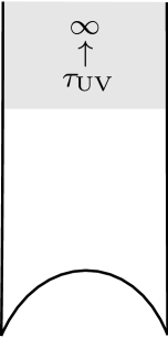
Figure 3: The marginal coupling $\tau_{\rm UV}$ in the Nekrasov partition function defines a local coordinate on the moduli space of the ${\cal N}=2$ conformal gauge theory near a weak-coupling point where $\tau_{\rm UV}\to\infty$.

In fact, it is not quite obvious that the full Nekrasov partition functions, in contrast to just the prepotential, should agree when expressed in the period matrix $\tau_{\rm IR}$. It would have been possible that the relation between the prepotential $\tau_{\rm IR}$ and the microscopic couplings $\tau_{\rm UV}$ gets quantum corrections in terms of the deformation parameters $\epsilon_{1}$ and $\epsilon_{2}$, in such a way that only when expressed in terms of a quantum period matrix $\tau_{\rm IR}(\epsilon_{1},\epsilon_{2})$ the Nekrasov partition functions do agree. In subsection 2.3 we will find however that this is not the case. The Nekrasov partition function agree when expressed in terms of the classical period matrix $\tau_{\rm IR}$. One possible argument for this is that the higher genus free energies ${\cal F}_{g\geq 1}$ are uniquely determined given the prepotential ${\cal F}_{0}$. In other words, that when the prepotentials (and thus Seiberg-Witten curves plus differentials) for two gauge theories agree we also expect the higher genus free energies to match up. This is reasonable to expect from several points of view, i.e. the interpretation of the ${\cal F}_{g}$’s as free energies in an integrable hierarchy [36, 37].

The Nekrasov partition function is computed as a series expansion in $q=\exp(2\pi i\tau_{UV})$. The microscopic coupling $\tau_{UV}$ thus corresponds to a choice of local coordinate on the moduli space of microscopic gauge couplings near a weak-coupling point (see Figure 3). An inequivalent renormalization scheme corresponds to a different choice of coordinate in that neighborhood. In particular, given two different renormalization schemes, by combining their respective IR-UV relations, we can obtain the relation between the two different microscopic couplings, and thus find the explicit coordinate transformation on the moduli space. Explicitly, we identify the infra-red couplings of two related theories by

$$\tau_{\rm IR}=\frac{1}{2}\partial_{a}^{2}{\cal F}_{0}^{A}(\tau_{\rm UV}^{A},a)=\frac{1}{2}\partial_{a}^{2}{\cal F}_{0}^{B}(\tau_{\rm UV}^{B},a).$$ (12)

By inverting the IR-UV relation for the gauge theory characterized by the microscopic coupling $\tau^{A}_{\rm UV}$, we find the relation between the microscopic couplings $\tau^{A}_{\rm UV}$ and $\tau^{B}_{\rm UV}$ of both gauge theories. Since this is a relation between quantities in the ultra-violet, we expect it to be independent of infra-red parameters such as the masses and Coulomb branch parameters. Indeed, in all examples that we study in subsection 2.3, we will find that the moduli-independent UV-UV relation that follows from equation (12) relates the Nekrasov partition functions up to a spurious factor that is independent of the Coulomb parameters.

We will often consider gauge theories as being embedded in string theories. Different models of the same gauge theory give different embeddings in string theory, which means that the results will differ when expressed in terms of UV variables, even though the IR results agree.

Take as an example the string theory realization of a supersymmetric ${\cal N}=2$ $SU(2)$ gauge theory. The unitary point of view leads to a construction of D4, NS5 and D6-branes in type IIA theory [13], whereas the symplectic point of view introduces an orientifold in this picture and mirror images for all D4-branes [41, 42, 43]. Clearly, these are different realizations of the $SU(2)$ gauge theory. Nevertheless, both descriptions should give the same result in the infra-red.

Indeed, the two aforementioned string theory embeddings, based on either a $U(2)$ or a $Sp(1)$ gauge group, determine a physically equivalent Seiberg-Witten curve. For instance, the brane embedding of the pure $Sp(1)$ gauge theory determines the curve [42]

$$s^{2}-s\left(v^{2}(v^{2}+u)+2\Lambda^{4}\right)+\Lambda^{8}=0,$$ (13)

in terms of the covering space variables $s\in\mathbb{C}^{*}$, $v\in\mathbb{C}$ and the gauge invariant coordinate $u={\rm Tr}(\Phi^{2})$ on the Coulomb branch. This is merely a double cover [44] of the more familiar parametrization of the $SU(2)$ Seiberg-Witten curve

$$\Lambda^{2}t^{2}-t\left(w^{2}+u\right)+\Lambda^{2}=0,$$ (14)

with $t\in\mathbb{C}^{*}$ and $w\in\mathbb{C}$, which follows from the unitary brane construction [13].

In fact, the choice for an instanton renormalization scheme is closely related to the choice for a brane embedding, as the precise parametrizations of the Seiberg-Witten curves (13) and (14) can be recovered in a thermodynamic (classical) limit by a saddle-point approximation of the $Sp(1)$ and the $U(2)$ Nekrasov partition functions respectively [33, 26].

2.3 Examples

Let us illustrate the above theory by a selection of examples. We start with comparing $Sp(1)/SO(4)$ and $U(2)$ partition functions in gauge theories with a single gauge group, and extend this to partition functions for more general linear and cyclic quivers. In particular, we find the identification of $Sp(1)/SO(4)$ and $U(2)$ instanton partition functions expressed in low-energy moduli and the relation between the $Sp(1)/SO(4)$ and $U(2)$ microscopic gauge couplings.

2.3.1 $Sp(1)$ versus $U(2)$ : the asymptotically free case

First of all, let us consider the $Sp(1)$ theory with a single gauge group coupled to $N_{f}$ massive hypermultiplets, where $N_{f}$ runs from 1 to 4. In the asymptotically free theories, with $N_{f}\leq 3$, we find that the $Sp(1)$ Nekrasov partition function equals the $U(2)$ Nekrasov partition function – with Coulomb parameters $(a,-a)$ – up to a factor that doesn’t depend on the Coulomb parameter and only contributes to the low genus refined free energies ${\cal F}_{0,\frac{1}{2},1}$. In the following we will call a factor with these two properties a spurious factor.

More precisely, we compute that

$$Z^{N_{f}=0}_{U(2)}(q)=Z^{N_{f}=0}_{Sp(1)}(q)$$ (15)

$$Z^{N_{f}=1}_{U(2)}(q)=Z^{N_{f}=1}_{Sp(1)}(q)$$ (16)

$$Z^{N_{f}=2}_{U(2)}(q)=Z^{N_{f}=2}_{Sp(1)}(q)[Z_{U(1)}^{\tilde{N}_{f}=0}(q)]^{1/2}$$ (17)

$$Z^{N_{f}=3}_{U(2)}(q)=Z^{N_{f}=3}_{Sp(1)}(q)[Z_{U(1)}^{\tilde{N}_{f}=1}(q)]^{1/2}\exp\left(-\frac{q^{2}}{32\epsilon_{1}\epsilon_{2}}\right),$$ (18)

up to degree six in the $q=\Lambda^{4-N_{f}}$ expansion, where $Z_{U(1)}^{\tilde{N}_{f}}$ is the instanton partition function of the $U(1)$ gauge theory coupled to $\tilde{N}_{f}$ hypermultiplets with masses $m_{1}$ up to $m_{\tilde{N}_{f}}$. Explicitly,

$$Z_{U(1)}^{\tilde{N}_{f}=0}(q)=\exp\left(-\frac{q}{\epsilon_{1}\epsilon_{2}}\right),$$ (19)

$$Z_{U(1)}^{\tilde{N}_{f}=1}(q)=\exp\left(-\frac{mq}{\epsilon_{1}\epsilon_{2}}\right),$$ (20)

with $q=\Lambda^{2-\tilde{N}_{f}}$, $m=\mu_{1}+\mu_{2}+\mu_{3}+\epsilon_{1}+\epsilon_{2}$ where $\mu_{i}$ being the masses of the fundamental hypermultiplets in equation (18). Note that the equalities (15)–(18) can equally well be written down for any combination of hypers in the fundamental and anti-fundamental representation of the $U(2)$ gauge group. The contribution of a fundamental hypermultiplet just differs from that of an anti-fundamental hypermultiplet by mapping $\mu\mapsto-\mu$.

Let us make two more remarks about the formulas (15)–(18). First, the form of the spurious factor in the equalities (15)–(18) is close to what is called the $U(1)$ factor in the AGT correspondence: they agree for $N_{f}=2$ and differ slightly for the $N_{f}=3$ theory. In particular, both factors don’t depend on the Coulomb parameters and only contribute to the lowest genus contributions ${\cal F}_{0,\frac{1}{2},1}$ of the refined free energy. Second, since the $U(2)$ and $Sp(1)$ Nekrasov partition functions coincide up to moduli-independent terms, the relation between IR and UV couplings is the same. It follows that they will agree up to spurious factors even when written in terms of IR couplings.

2.3.2 $Sp(1)$ versus $U(2)$ : the conformal case

Figure 4: On the left: Quiver of the $Sp(1)$ gauge theory coupled to two fundamental and two anti-fundamental hypermultiplet. Since the (anti-)fundamental representation of $Sp(1)$ is pseudo-real, the flavor symmetry group of two hypermultiplets enhances to $SO(4)$. On the right: Quiver of the $SU(2)$ gauge theory coupled to two fundamental and two anti-fundamental hypermultiplets. The flavor symmetries of the hypermultiplets is enhanced to $SU(2)$.

Comparing the Nekrasov partition functions for conformal $Sp(1)$ and the $U(2)$ gauge theories, both coupled to four hypermultiplets, yields a substantially different result.^, (The quivers of the respective gauge theories are illustrated in Figure 4 for later reference.) The $Sp(1)$ Nekrasov partition function does not agree with the $U(2)$ Nekrasov partition function up to a spurious factor, when expressed in the UV gauge couplings with the identification $q_{Sp(1)}=q_{U(2)}$. In particular, the prepotentials ${\cal F}_{0}$ differ, leading to a different relation between $\tau_{\rm IR}$ and $q_{Sp(1)}$ than between $\tau_{\rm IR}$ and $q_{U(2)}$.

When all the hypers are massless, or equivalently when sending the Coulomb parameter $a\to\infty$, we find that the map between UV gauge couplings and the period matrix $\tau_{\rm IR}$ does not depend on $a$ and is given by ^,

$$q_{Sp(1)}^{2} =16\,\frac{\theta_{2}(q_{\rm IR}^{2})^{4}}{\theta_{3}(q_{\rm IR}^{2})^{4}}$$ (21)

$$q_{U(2)} =\frac{\theta_{2}(q_{\rm IR})^{4}}{\theta_{3}(q_{\rm IR})^{4}},$$ (22)

where we define $q_{\rm IR}=\exp(2\pi i\tau_{\rm IR})$. The $Sp(1)$ and $U(2)$ mappings just differ by doubling the value of the microscopic gauge coupling as well as the infra-red period matrix.

If we express the massless partition functions in terms of the low-energy variables by using (21) and (22), they agree up to a spurious factor (which is independent of the Coulomb parameter $a$ and only contributes to the lower genus refined free energies ${\cal F}_{0,\frac{1}{2},1}$). In fact, it turns out that even if we re-express the massive partition functions using the massless UV-IR mappings (21) and (22), we still find agreement up to a spurious factor.

On the other hand, even if we use the massive $Sp(1)$ and $U(2)$ IR-UV mappings which do depend on the Coulomb parameter $a$ and the masses of the hypers, we find that the $Sp(1)$ and $U(2)$ renormalization scheme are related by the transformation

$$\boxed{q_{U(2)}=q_{Sp(1)}\left(1+\frac{q_{Sp(1)}}{4}\right)^{-2},}$$ (23)

which as expected is not dependent on the Coulomb branch moduli.

For completeness let us give the expression for the spurious factor once we express both full partition functions in terms of $q_{Sp(1)}$. For the unrefined case $\hbar=\epsilon_{1}=-\epsilon_{2}$ we find

$$\frac{Z_{U(2)}(q_{U(2)}(q_{Sp(1)}))}{Z_{Sp(1)}(q_{Sp(1)})}=\left(1+\frac{q_{Sp(1)}}{4}\right)^{M+N}\left(1-\frac{q_{Sp(1)}}{4}\right)^{N-M},$$ (24)

where $M=\frac{1}{\hbar^{2}}\sum_{i<j}\mu_{i}\mu_{j}$ and $N=-\frac{1}{2\hbar^{2}}\sum_{i}\mu_{i}^{2}+\frac{1}{8}$. Here, we emphasize that this relation is between the full Nekrasov partition functions including the perturbative pieces and not just between the instanton parts. Notice that this spurious factor is quite close to, yet more complicated than the square-root of the unrefined $U(1)$ partition function

$$Z_{U(1)}^{N_{f}=2}(q)=\left(1-q\right)^{-\frac{m_{1}m_{2}}{\hbar^{2}}},$$

of the $U(1)$ gauge theory coupled to two hypermultiplets with masses $m_{1}$ and $m_{2}$, the square of which entered the AGT correspondence as the “$U(1)$ factor”. Similarly, we interpret the spurious factor (24) as a decoupled $U(1)$ factor.

2.3.3 $SO(4)$ versus $U(2)\times U(2)$ instantons

The instanton partition function for the pure $SO(4)$ gauge theory agrees with that of the pure $U(2)\times U(2)$ theory

$$Z_{SO(4)}^{N_{f}=0}(q)=Z_{U(2)\times U(2)}^{N_{b}=0}(q)\ ,$$ (25)

if we make the identifications

$$q_{U(2),1}=q_{U(2),2}=16\ q_{SO(4)}\quad\mbox{and}\quad(b_{1},b_{2})=(a_{1}+a_{2},a_{1}-a_{2})\ .$$ (26)

Here, $b_{1,2}$ are the Coulomb parameters of the $SO(4)$ gauge theory and $a_{1.2}$ those of the $U(2)\times U(2)$ gauge theory. The second relation follows simply from the embedding of $\mathfrak{su}(2)\times\mathfrak{su}(2)$ in $\mathfrak{so}(4)$.

When we couple the $SO(4)$ theory to a single massive hypermultiplet, its instanton partition function matches with that of the $U(2)\times U(2)$ theory coupled to a massive bifundamental up to a spurious factor

$$Z_{SO(4)}^{N_{f}=1}(q)=Z_{U(2)\times U(2)}^{N_{b}=1}(q)\exp\left(-\frac{4q}{\hbar^{2}}\right),$$ (27)

for the unrefined case under the same identification (26).

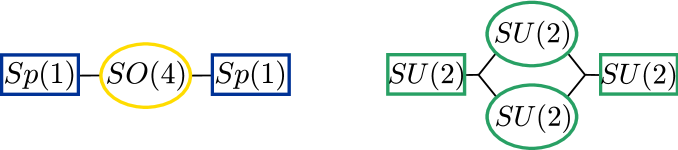
Figure 5: On the left: Quiver representation of the $SO(4)$ gauge theory coupled to one fundamental and one anti-fundamental hypermultiplet. Since the (anti-)fundamental representation of $SO(4)$ is real, the flavor symmetry group of each hypermultiplet enhances to $Sp(1)$. On the right: Quiver representation of the $SU(2)\times SU(2)$ gauge theory coupled to two bi-fundamental hypermultiplets. The flavor symmetry of the bifundamental field is enhanced to $SU(2)$.

Now, let us consider the conformal case. Naively comparing the Nekrasov partition function of the conformal $SO(4)$ gauge theory coupled to two massive hypermultiplets with that of the $U(2)\times U(2)$ theory coupled by two massive bifundamentals shows a serious disagreement. (Their quivers are illustrated in Figure 5.) However, if we follow the same strategy as explained in the conformal $Sp(1)$ example, we see that it is once more simply a matter of different renormalization schemes. The $SO(4)$ and the $U(2)$ gauge theory are related by the change of marginal couplings

$$\boxed{q_{SO(4)}=\frac{\theta_{2}(q_{U(2)})^{4}}{\theta_{3}(q_{U(2)})^{4}},}$$ (28)

when we identify $q_{U(2)}=q_{U(2),1}=q_{U(2),2}$. Using this UV-UV relation and the relation between the Coulomb branch parameters (26), the $SO(4)$ and $U(2)\times U(2)$ Nekrasov partition functions agree up to a spurious factor

$$\frac{Z_{U(2)\times U(2)}(q_{U(2)}(q_{SO(4)}))}{Z_{SO(4)}(q_{SO(4)})}=1-\frac{4M}{\hbar^{2}}q+\frac{8M^{2}+2N\hbar^{2}}{\hbar^{4}}q^{2}+\ldots$$ (29)

that is similar to the $Sp(1)-U(2)$ spurious factor in equation (24), with now $M=m_{1}^{2}-m_{1}m_{2}+m_{2}^{2}$ and $N=3m_{1}^{2}+m_{1}m_{2}+3m_{2}^{2}$.

2.3.4 $Sp(1)\times Sp(1)$ versus $U(2)\times U(2)$ instantons

Next, we analyze $Sp(1)\times Sp(1)$ quiver gauge theories coupled to at most 4 massive hypermultiplets. The bifundamental multiplet, that couples the two $Sp(1)$ gauge groups, introduces new poles in the theory, similar to the adjoint multiplet in the ${\cal N}=2^{*}$ gauge theory.

As expected, we find immediate agreement between the $Sp(1)$ and $U(2)$ instanton partition functions up to a spurious factor, when we couple fewer than two hypers to each multiplet.

If more than two hypers are coupled to one of the gauge groups, we need to express the partition function in terms of the physical period matrix $\tau_{\rm IR}$. Notice that the $Sp(1)$ (as well as $U(2)$) instanton partition function is a function of two UV gauge couplings, whereas the period matrix is a symmetric $3\times 3$ matrix. It is nevertheless easy to find a bijective relation between the two diagonal entries of the period matrix and the two UV gauge couplings. The off-diagonal entry in the period matrix represents a mixing of the two gauge groups, and can be expressed in terms of the diagonal entries.

Let us consider the conformal linear quiver with two $Sp(1)$ gauge groups as an example. We couple the two $Sp(1)$’s by a bifundamental and add two extra hypermultiplets to the first and to the second gauge group. The moduli-independent UV-IR relation for $Sp(1)$ has a series expansion

$$q_{Sp(1),i} =q_{\mathrm{IR},ii}-\frac{1}{64}q_{\mathrm{IR},ii}^{3}+\frac{1}{32}\ q_{\mathrm{IR},ii}q_{\mathrm{IR},jj}^{2}+{\cal O}(q_{\mathrm{IR}}^{4}),$$ (30)

whereas the one for $U(2)$ has the form

$$q_{U(2),i} =q_{\mathrm{IR},ii}-\frac{1}{2}q_{\mathrm{IR},ii}^{2}+\frac{1}{2}q_{\mathrm{IR},ii}q_{\mathrm{IR},jj}+\frac{11}{64}q_{\mathrm{IR},ii}^{3}$$

$$\quad-\frac{1}{2}q_{\mathrm{IR},ii}^{2}q_{\mathrm{IR},jj}+\frac{3}{32}q_{\mathrm{IR},ii}q_{\mathrm{IR},jj}^{2}+{\cal O}(q_{\mathrm{IR}}^{4}),$$ (31)

for $i\in\{1,2\}$ and $i\neq j$.

As before we use the moduli-independent UV-IR mappings (30) and (31) to evaluate the massive partition function as a function of the physical IR moduli $\tau_{\rm IR,11}$ and $\tau_{\rm IR,22}$. Again this shows agreement of the $Sp(1)$ and $U(2)$ partition functions up to a spurious factor in the lower genus free energies.

Composing the moduli-dependent mappings between UV-couplings and the period matrix, we find that the two renormalization schemes are related by

$$q_{Sp(1),i} =q_{U(2),i}+\frac{1}{2}q_{U(2),i}^{2}-\frac{1}{2}q_{U(2),i}q_{U(2),j}+\frac{5}{16}q_{U(2),i}^{3}$$

$$\quad-\frac{1}{16}q_{U(2),i}q_{U(2),j}^{2}+{\cal O}(q_{U(2)}^{4}),$$ (32)

for $i\in\{1,2\}$ and $i\neq j$. Note that this mapping is independent of the Coulomb branch moduli and the mass parameters, as it should be. Notice as well that a mixing amongst the two gauge groups takes places, so that we cannot simply use the UV-UV mapping for a single gauge group twice. Substituting this relation into the $Sp(1)$ partition function indeed turns brings it into the form of the $U(2)$ partition function up to a spurious AGT-like factor.

The above procedure can be applied to any linear or cyclic quiver. Most importantly, the $Sp(1)$ and $U(2)$ partition function agree (up to a spurious factor) when expressed in IR coordinates, and, the mapping between $Sp(1)$ and $U(2)$ renormalization schemes is independent of the moduli in the gauge theory and mixes the gauge groups. Moreover, the spurious factors that we find are more complicated than the “$U(1)$-factors” that appear in the AGT correspondence.

3 ${\cal N}=2$ geometry

In section 2 we found in which way Nekrasov partition functions for different models of the same underlying physical gauge theory are related, i.e. comparing the $U(2)$ versus the $Sp(1)$ method of instanton counting. The ${\cal N}=2$ instanton counting defines a renormalization scheme for each model, such that, when expressed in terms of physical infra-red variables, the Nekrasov partition functions of two such models agree up to a spurious factor. When expressed in terms of the microscopic couplings, however, the Nekrasov partition functions are related by a non-trivial mapping. Our goal in this section is to explain this mapping geometrically.

The previous section contained a brief review of the low energy data contained in the Seiberg-Witten curve. As expected we were able to verify that physically relevant quantities agree for different models of the same low energy gauge theory. In [1] it was shown how to extract additional information from the Seiberg-Witten curve beyond the low energy data. This information is encoded in a realization of the Seiberg-Witten curve as a branched cover over yet another punctured Riemann surface, which we will refer to as the Gaiotto curve (or G-curve).

As we review in more detail in a moment, the branched cover realization can be read off from the brane construction of the ${\cal N}=2$ gauge theory. The number of D4-branes that is necessary to engineer the gauge theory determines the degree of the covering. Branch points of the covering (which are punctures on the Gaiotto curve) correspond to poles in the Seiberg-Witten differential, and their residues are associated to the bare mass parameters in the gauge theory.

In [1] the complex structure moduli of the Gaiotto curve are identified with the exactly marginal couplings of the conformal ${\cal N}=2$ gauge theory. The Gaiotto curve therefore not only captures the infra-red data of the gauge theory, but also information about the chosen renormalization scheme. Different renormalization schemes are related by non-trivial mappings of exactly marginal couplings. Geometrically, it was argued that a choice of renormalization scheme corresponds to a choice of local coordinates on the complex structure moduli space of the Gaiotto curve.

A given physical gauge theory of course admits a countless number of renormalization schemes. On the other hand, our focus in this paper is only to find a geometric interpretation of a small subset of such choices. We expect to find such an interpretation when different models can both be embedded by a brane construction in string theory. In such examples we can construct the corresponding Gaiotto curves and a mapping between them. This mapping geometrizes the mapping between the exactly marginal couplings.

Most of the examples we considered in the previous section are of this type. However, one of them is not. This is the comparison of the $SU(2)\times SU(2)$ gauge theory with the $Sp(1)\times Sp(1)$ gauge theory. Since we are not aware of a brane embedding of the latter theory, there is no immediate reason to expect an (obvious) geometric interpretation of the mapping between exactly marginal couplings in that example. In the other examples, for which brane constructions are well-known, we do expect to find a geometric explanation for the UV-UV mappings.

As a last comment, let us emphasize that the validity of the mappings between exactly marginal couplings extends beyond the prepotential ${\cal F}_{0}$. As we found in the last section, the full Nekrasov partition functions $Z^{\rm Nek}$ are related by the mapping between UV couplings, which does not receive corrections in the deformation parameters $\epsilon_{1}$ and $\epsilon_{2}$. Geometrically, this implies that there are no quantum corrections to the mappings between the Gaiotto curves for different models of the same physical gauge theory.

In this section we start by reviewing the construction of Gaiotto curves for ${\cal N}=2$ gauge theories with a classical gauge group. We explain how the ${\cal N}=2$ geometry is encoded in a ramified Hitchin system whose base is the Gaiotto curve. Furthermore, we make some comments on its six-dimensional origin. We then compare geometric realizations for unitary and symplectic/orthogonal gauge theories. In particular, we argue how different models of the same theory are related geometrically. We explicitly verify this in some examples, where we compare the geometry underlying $Sp(1)$ and $SO(4)$ quiver gauge theories to those of $U(2)$ quivers. As expected, we find a geometric explanation for the relation between the marginal couplings that we computed in the previous section.

3.1 G-curves and Hitchin systems

Let us start this section with reviewing the constructions of Gaiotto curves for $SU(N)$ and $Sp(N)/SO(N)$ gauge groups and their embedding in a ramified Hitchin system. We then explain how to compare them in specific cases.

3.1.1 Unitary gauge group

Figure 6: Illustrated on the left is an example of a D4/NS5 brane construction realizing the $SU(2)$ quiver gauge theory illustrated on the right. The Coulomb and mass parameters of the $SU(2)$ gauge theory parametrize the separation of the D4-branes, while the separation of the NS5-branes determines the microscopic coupling $\tau_{\rm UV}$. The Seiberg-Witten curve for this $SU(2)$ gauge theory is a torus with complex structure parameter $\tau_{\rm IR}$.

A special unitary quiver gauge theory can be realized in type IIA string theory using a D4/NS5 brane embedding [13]. See Figure 6 for the brane embedding of the $SU(2)$ gauge theory coupled to four hypermultiplets. From such a brane embedding one can read off the Seiberg-Witten curve $\Sigma$ of the quiver gauge theory. It is, roughly speaking, a fattening of the D4/NS5 graph, as it is for instance illustrated in Figure 6.

The D4/NS5 brane embedding can be lifted to an M5-brane embedding in M-theory. The resulting ten-dimensional M-theory background is

$$\mathbb{R}^{4}\times T^{*}\tilde{C}\times\mathbb{R}^{2}\times S^{1},$$ (33)

where we introduced a possibly punctured Riemann surface $\tilde{C}$ and its cotangent bundle $T^{*}\tilde{C}$. We insert a stack of $N$ M5-branes that wraps the six-dimensional manifold $\mathbb{R}^{4}\times\tilde{C}$. The positions of these M5-branes in the cotangent bundle determine the Seiberg-Witten curve $\Sigma$ as a subspace of $T^{*}\tilde{C}$. In this perspective the Seiberg-Witten curve is given [1]

$$0={\rm det}(w-\boldsymbol{\phi}_{U})=w^{N}+w^{N-2}\phi_{2}+w^{N-3}\phi_{3}+\ldots+\phi_{N}$$ (34)

as a branched degree $N$ covering over the so-called Gaiotto curve $\tilde{C}$. The holomorphic differential $w$ parametrizes the fiber direction of the cotangent bundle $T^{*}\tilde{C}$, whereas $\boldsymbol{\phi}_{U}$ is an $SU(N)$-valued differential on the curve $\tilde{C}$ of degree 1.

The degree $d$ differentials $\phi_{d}={\rm Tr}(\boldsymbol{\phi}_{U}^{d})$ encode the classical vev’s of the $SU(N)$ Coulomb branch operators of dimension $d$. They are allowed to have poles at the punctures of the Gaiotto curve. The coefficients at these poles encode the bare mass parameters of the gauge theory. To take care of these boundary conditions in the M-theory set-up, we need to insert additional M5-branes at the punctures of the Gaiotto curve. These M5-branes should intersect the Gaiotto curve transversally, and thus locally wrap the fiber of the cotangent bundle at the puncture [46].

Equation (34) determines the Seiberg-Witten curve $\Sigma$ as an $N$-fold branched covering over the Gaiotto curve $\tilde{C}$. The Seiberg-Witten differential is simply

$$\lambda=w.$$ (35)

The ${\cal N}=2$ geometry for unitary gauge groups is thus encoded in a ramified $A_{N}$ Hitchin system on the punctured Gaiotto curve $\tilde{C}$, whose spectral curve is the Seiberg-Witten curve $\Sigma$ and whose canonical 1-form is equal to the Seiberg-Witten differential [47].

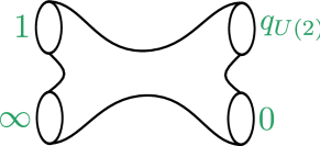
Figure 7: The left Figure illustrates the Gaiotto curve $\tilde{C}$ of the conformal $SU(2)$ quiver gauge theory that is illustrated on the right. The Gaiotto curve is a four-punctured sphere with complex structure parameter $q_{U(2)}$. The differential $\phi_{2}$ has second order poles at the four punctures. The $SU(2)$ flavor symmetries are encoded in the coefficients of the differential $\phi_{2}$ at these poles.

The topology of the Gaiotto curve is fully determined by the corresponding quiver diagram. A gauge group translates into a tube of the Gaiotto curve, whereas a flavor group turns into a puncture. This is illustrated in Figure 7 for the $SU(2)$ gauge theory coupled to four flavors. The poles of the differentials $\phi_{d}$ determine the branch points of the fibration (34). Their coefficients encode the flavor symmetry of the quiver gauge theory. For gauge group $SU(N)$ the degree of the poles is integer. As we will see shortly this is not true for $Sp(N)$ and $SO(N)$ gauge theories.

3.1.2 Symplectic/orthogonal gauge group

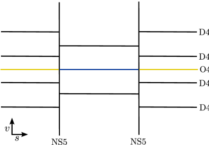
Figure 8: Illustrated on the left is an example of a D4/NS5 brane construction with O4^± orientifold branes realizing the $Sp(1)$ quiver gauge theory illustrated on the right. The O4^- branes (in yellow) ensure that both flavor symmetry groups are $SO(4)$, whereas the O4⁺ brane (in blue) ensures that the gauge symmetry group is $Sp(1)$. The brane embedding of the conformal $SO(4)$ gauge theory is found by swapping the inner and the outer D4 and O4 branes.

For symplectic or orthogonal gauge theories a similar description exists. Engineering these gauge theories in type IIA requires orientifold O4-branes in addition to the D4 and NS5-branes [41, 42, 43]. The orientifold branes are parallel to the D4 branes. They act on the string background as a combination of a worldsheet parity $\Omega$ and a spacetime reflection in the five dimensions transverse to it. The space-time reflection introduces a mirror brane for each D4-brane, whereas the worldsheet parity breaks the space-time gauge group. More precisely, there are two kinds of O4-branes, distinguished by the sign of $\Omega^{2}=\pm 1$. The O4^- brane breaks the $SU(N)$ gauge symmetry to $SO(N)$, whereas the O4⁺ brane breaks it to $Sp(N/2)$. The brane construction that engineers the conformal $Sp(1)$ gauge theory is schematically shown in Figure 8. Notice that there are two hidden D4-branes on top of the O4⁺ brane, so that the number of D4-branes is equal at each point over the base.

From these brane setups we can extract the Seiberg-Witten curve for the $Sp(N-1)$ and $SO(2N)$ gauge theories coupled to matter. To find the Gaiotto curve we rewrite the Seiberg-Witten curve in the form [48]

$$0=v^{2N}+\varphi_{2}v^{2N-2}+\varphi_{4}v^{2N-4}+\ldots+\varphi_{2N},$$ (36)

where the differentials $\varphi_{k}$ encode the Coulomb parameters and the bare masses. Equation (36) defines the Seiberg-Witten curve as a branched covering over the $Sp/SO$ Gaiotto curve. More precisely, the Seiberg-Witten curve is embedded in the cotangent bundle $T^{*}C$ of the Gaiotto curve $C$ with holomorphic differential $v$. The Seiberg-Witten differential is simply

$$\lambda=v,$$ (37)

the canonical 1-form in the cotangent bundle $T^{*}C$.

Whereas for the $Sp(N-1)$ gauge theory there is an extra condition saying that the zeroes at $v=0$ of the right-hand-side should be double zeroes, the $SO(2N)$ gauge theory requires these zeroes to be simple zeroes. These conditions come up somewhat ad-hoc in the type IIA description, but can be explained from first principles in an M-theory perspective [49]. The orientifold brane construction lifts in M-theory to a stack of M5-branes in a $\mathbb{Z}_{2}$-orbifold background. The orbifold acts on the five dimensions transverse to the M5-branes, and in particular maps $v\mapsto-v$.

For the pure $Sp(N-1)$-theory the differential $\varphi_{2N}$ vanishes, so that a factor $v^{2}$ in equation (36) drops out. The resulting Seiberg-Witten curve can be written in the form

$$0={\rm det}(v-\boldsymbol{\varphi}_{Sp}),$$ (38)

where $\boldsymbol{\varphi}_{Sp}$ is a $Sp(N-1)$-valued differential. The non-vanishing differentials $\varphi_{2k}$ can thus be obtained from the Casimirs of the Lie algebra $\mathfrak{sp}(N-1)$. If we include massive matter to the $Sp(N-1)$ gauge theory, however, or consider an $SO(2N)$ gauge theory, equation (36) can be reformulated as

$$0={\rm det}(v-\boldsymbol{\varphi}_{SO})$$ (39)

where the differential $\boldsymbol{\varphi}_{SO}$ is $SO(2N)$-valued. This equation is clearly characterized by the Casimirs of the Lie algebra $\mathfrak{so}(2N)$. More precisely, we recognize the $D_{N}$-invariants ${\rm Tr}(\Phi^{2k})$ and $\mathrm{Pfaff}(\Phi)$ in the differentials $\varphi_{2k}$ and $\varphi_{\tilde{N}}=\sqrt{\varphi_{2N}}$, respectively. In general, the ${\cal N}=2$ geometry for symplectic and orthogonal gauge groups is thus encoded in a ramified $D_{N}$ Hitchin system based on the $Sp/SO$ Gaiotto curve $C$, whose spectral curve is the Seiberg-Witten curve (36).

The Lie algebra $D_{N}$ has a $\mathbb{Z}_{2}$ automorphism under which the invariants with exponent $2,\ldots,2N-2$ are even and the invariant of degree $N$ is odd. On the level of the differentials $\phi_{k}$ this translates into possible half-integer poles for the invariant $\varphi_{\tilde{N}}$. Going around such a pole the differential $\varphi_{\tilde{N}}$ has a $\mathbb{Z}_{2}$ monodromy. We will see explicitly in the examples. We call the puncture corresponding to such a pole a half-puncture. The half-punctures introduce $\mathbb{Z}_{2}$ twist-lines on the Gaiotto curve [48]. This is illustrated for the $Sp(1)$ and $SO(4)$ Gaiotto curve in Figure 9 and Figure 10.

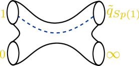
Figure 9: The left Figure illustrates the Gaiotto curve $C$ of the conformal $Sp(1)$ quiver gauge theory that is illustrated on the right. The $Sp(1)$ Gaiotto curve differs from the $SU(2)$ Gaiotto curve by the $\mathbb{Z}_{2}$ twist-line that runs parallel to the tube. We will discuss the precise relation between the $Sp(1)$ and the $SU(2)$ Gaiotto curve in section 3.2.

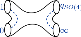
Figure 10: The left Figure illustrates the Gaiotto curve $C$ of the conformal $SO(4)$ quiver gauge theory that is illustrated on the right. The $SO(4)$ Gaiotto curve differs from the $Sp(1)$ Gaiotto curve by a different configuration of $\mathbb{Z}_{2}$ twist-lines. In particular, the twist lines don’t run through the tube.

Lastly, let us make a few remarks on the worldvolume theory on a stack of M5-branes. In the low energy limit this theory is thought to be described by a six-dimensional conformal $(2,0)$ theory of type $ADE$. For the M-theory background (33) it is of type $A$, whereas for the $\mathbb{Z}_{2}$-orbifolded M-theory background it is of type $D$. The $(2,0)$ theory has a “Coulomb branch” parametrized by the vev’s of a subset of chiral operators whose conformal weights are given by the exponents $d$ of the Lie algebra $\mathfrak{g}$. These operators parametrize the configurations of M5-branes in the M-theory background. In the Hitchin system they appear as the degree $d$ differentials. Boundary conditions at the punctures of the Gaiotto curve are expected to lift to defect operators in the M5-brane worldvolume theory. We refer to [46] for a more detailed description.

3.1.3 $SO/Sp$ versus $U$ geometries

Suppose that we have two models for the same physical gauge theory, who both can be embedded as a ramified Hitchin system in M-theory. How are these models related geometrically?

First of all, we expect that the mapping between the exactly marginal couplings is reflected as a mapping between the complex structure parameters of the corresponding Gaiotto curves. Also, there should be an isomorphism between the spectral curves of the respective Hitchin systems, as these correspond to the Seiberg-Witten curves. Moreover, the boundary conditions of the Hitchin differentials at the punctures of both models should be related by the mapping that identifies the corresponding matter representations. In particular, this relates the eigenvalues of the Seiberg-Witten differential at the punctures of both models. In total we should thus find a bijective mapping between the complete ramified Hitchin system, including the Gaiotto curve as well as the Hitchin differentials.

As we will see in detail in the next subsection, it is easy to come up with such a mapping for $Sp(1)/SO(4)$ versus $SU(2)$ gauge theories [48]. We just interpret the $\mathbb{Z}_{2}$-twist lines on the $Sp(1)/SO(4)$ Gaiotto curve as branch-cuts, and its double cover as the $SU(2)$ Gaiotto curve. The latter curve is thus equipped with an involution that interchanges the two sheets of the cover. We can recover the Hitchin differentials on the $Sp(1)/SO(4)$ Gaiotto curve by splitting the Hitchin differential on its cover into even and odd parts under the involution. Indeed, recall that the $SU(2)$ Seiberg-Witten curve is determined by a single differential $\phi_{2}$ of degree 2, whereas the $Sp(1)/SO(4)$ Seiberg-Witten curve is defined by two degree 2 differentials $\varphi_{2}$ and $\varphi_{\tilde{2}}$, the first one being even under the $\mathbb{Z}_{2}$-automorphism and the second one odd.

Notice that this double construction doesn’t work for any $Sp/SO$ theory, as the differentials on the cover generically do not have a simple interpretation in terms of a set of differentials of a unitary theory. Two theories can only be related by a double covering if the Lie algebra underlying the Hitchin system of one of them splits into two copies of the Lie algebra underlying the Hitchin system of the other. Nonetheless, for any two models of the same gauge theory there should be a corresponding isomorphism of Hitchin systems.

Before going into the example-subsection, let us note that in the previous section we also encountered a gauge theory without an obvious brane embedding. This is the $Sp(1)\times Sp(1)$ gauge theory. It is not possible to realize this theory in the standard manner using NS5-branes, as the type of the orientifold has to differ on either side of the NS5-brane. Geometrically, this is reflected in the fact that there doesn’t exist an involution on the $SU(2)\times SU(2)$ Gaiotto curve with the right properties. It would be interesting to find whether there exists a geometric interpretation of the mapping between the exactly marginal couplings of the $SU(2)\times SU(2)$ and the $Sp(1)\times Sp(1)$ gauge theory anyway.

3.2 Examples

Let us now return to the results of section 2. First of all, we can explain the appearance of the modular lambda function

$$\lambda=\frac{\theta_{2}^{4}}{\theta_{3}^{4}}:\mathbb{H}\to\mathbb{P}^{1}\backslash\{0,1,\infty\}$$ (40)

as the relation (22) between the infra-red coupling $\tau_{\rm IR}$ and the exactly marginal coupling $q_{U(2)}$ in the conformal $SU(2)$ gauge theory. This modular function gives an explicit isomorphism between the quotient $\mathbb{H}/\Gamma(2)$ of the upper half plane $\mathbb{H}$ by the modular group $\Gamma(2)$ and $\mathbb{P}^{1}\backslash\{0,1,\infty\}$. Whereas the complex structure modulus $\tau_{\rm IR}$ of the $SU(2)$ Seiberg-Witten curve takes values in $\mathbb{H}/\Gamma(2)$, the complex structure modulus $q_{U(2)}$ of the $SU(2)$ Gaiotto curve (which is the cross-ratio of the four punctures on the G-curve) takes values in $\mathbb{P}^{1}\backslash\{0,1,\infty\}$. The modular lambda function thus determines the double cover map between the Seiberg-Witten curve and the Gaiotto curve for the conformal $SU(2)$ gauge theory [2].

We continue with studying the $Sp(1)$ and $SO(4)$ geometry in detail. In appendix C we have summarized various existing descriptions of the $SU(2)$ geometry, and their relation to the Gaiotto geometry.

3.2.1 $Sp(1)$ versus $U(2)$ geometry

The $Sp(1)$ Seiberg-Witten curve can be derived from the orientifold brane construction that is illustrated in Figure 8. In Gaiotto form it reads

$$v^{4} =\varphi_{2}(s)v^{2}+\varphi_{4}(s)$$ (41)

with

$$\varphi_{2}(s) =\frac{(\mu_{1}^{2}+\mu_{2}^{2})s^{2}+u(1+\tilde{q}_{Sp(1)})s+(\mu_{3}^{2}+\mu_{4}^{2})\tilde{q}_{Sp(1)}}{\left(s-1\right)\left(s-\tilde{q}_{Sp(1)}\right)}\left(\frac{ds}{s}\right)^{2}$$

$$\varphi_{4}(s) =-\frac{\mu_{1}^{2}\mu_{2}^{2}s^{2}+2\prod_{i=1}^{4}\mu_{i}\sqrt{\tilde{q}_{Sp(1)}}s+\mu_{3}^{2}\mu_{4}^{2}\tilde{q}_{Sp(1)}}{\left(s-1\right)\left(s-\tilde{q}_{Sp(1)}\right)}\left(\frac{ds}{s}\right)^{4},$$

where $\mu_{i}$ are the bare masses of the hypermultiplets, and $u$ is the classical vev of the adjoint scalar $\Phi$ in the gauge multiplet. We also introduced a new parameter $\tilde{q}_{Sp(1)}$ that we will relate to the coupling $q_{Sp(1)}$ in a moment. The differential $\varphi_{2}$ corresponds to the $D_{2}$-invariant ${\rm Tr}(\Phi^{2})$, whereas the square-root $\varphi_{\tilde{2}}=\sqrt{\varphi_{4}}$ corresponds to the $D_{2}$-invariant $\rm{Pfaff}(\Phi)$. Note that the differential $\varphi_{4}$ vanishes if the masses are set to zero.

It follows that the $Sp(1)$ Seiberg-Witten curve is a branched fourfold cover over the G-curve $\mathbb{P}^{1}$ with coordinate $s$. The G-curve has four branch points at the positions

$$s\in\{0,\tilde{q}_{Sp(1)},1,\infty\},$$ (42)

The complex structure of the $Sp(1)$ Gaiotto curve is parametrized by $\tilde{q}_{Sp(1)}$. Since the differential $\varphi_{\tilde{2}}$ has a pole of order half at the punctures at $s=1$ and $s=\tilde{q}_{Sp(1)}$, these are half-punctures. There is a $\mathbb{Z}_{2}$-twist line running between the two half-punctures, as the differential $\varphi_{\tilde{2}}$ experiences a $\mathbb{Z}_{2}$ monodromy around them. In contrast, the punctures at $s=0$ and $s=\infty$ are full punctures.

The Seiberg-Witten differential $\lambda$ is a $SO(4,\mathbb{C})$-valued differential. It has nonzero residues at the poles $s=0$ and $s=\infty$ only. This implies that the $SO(4)$ flavor symmetry is associated with these punctures. Indeed, the residues of the differential $\lambda$ at $s=\infty$ are given by $\pm\mu_{1}$ and $\pm\mu_{2}$, whereas at $s=0$ they are $\pm\mu_{3}$ and $\pm\mu_{4}$. So both at $s=0$ and $s=\infty$ the residues parametrize the Cartan of $\mathfrak{su}(2)\times\mathfrak{su}(2)=\mathfrak{so}(4)$.

Summarizing, we have found that the $Sp(1)$ G-curve is a four-punctured two-sphere with two half-punctures and two full punctures. The two $SO(4)$-flavor symmetry groups can be associated to the two full punctures. This is illustrated in the left picture in Figure 9.

Viewing the $\mathbb{Z}_{2}$-twist lines as branch-cuts, and the half-punctures as branch-points, it is natural to consider the double cover of the G-curve. Let us use the $SL(2,\mathbb{C})$ freedom of the $Sp(1)$ theory to interchange the full-punctures with the half-punctures. Call the complex structure coordinate of the $Sp(1)$ G-curve $\tilde{q}_{Sp(1)}=q^{2}$. The branched covering map is then simply given by

$$t^{2}=s,$$

where $s$ is the coordinate on the $Sp(1)$ G-curve and $t$ the coordinate on the double cover. The pre-images of the full punctures on the base are at $\pm 1,\pm q$ on the cover, and there is a $SU(2)$-flavor symmetry attached to them. The total flavor symmetry at both full-punctures adds up to $SO(4)$. This is illustrated in Figure 11.

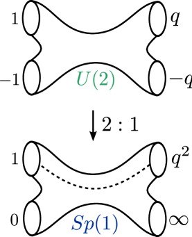
Figure 11: The G-curve of the $SU(2)$ gauge theory coupled to 4 hypers is a double cover over the G-curve of the $Sp(1)$ gauge theory with 4 hypers. We denote the complex structure parameter on the $Sp(1)$ Gaiotto curve by $\tilde{q}_{Sp(1)}=q^{2}$.

Note that this double cover of the $Sp(1)$ G-curve has exactly the same structure as the $SU(2)$ G-curve. The only difference is that the punctures are at different positions, something which can be taken care of by a Möbius transformation. Since this leaves the complex structure of the G-curve invariant, the gauge theory is invariant under such transformations. In particular the masses of the hypermultiplets, which are the residues of the Seiberg-Witten differential at its poles, remain the same. We can use the fact that the cross-ratios of the two configurations have to be equal to read off the relation between the $U(2)$ and $Sp(1)$ exactly marginal couplings,

$$\boxed{q_{U(2)}=4q\left(1+q\right)^{-2}.}$$ (43)

Explicitly, the Möbius transformation that relates the $SU(2)$ G-curve and the double cover of the $Sp(1)$ G-curve is given by the mapping

$$\gamma(z)=-\frac{z\left(1+q\right)-2q}{z\left(1+q\right)-2}\ ,$$ (44)

that sends the four punctures at positions $\{0,1,q_{U(2)},\infty\}$ to four punctures at the positions $\{\pm q,\pm 1\}$.

We can now make contact between the geometry of the $SU(2)$ and $Sp(1)$ Gaiotto curves and the relation between their exactly marginal couplings. Indeed, we recover the UV-UV mapping (23) from the identification of cross-ratios in equation (43), when we identify

$$\boxed{q^{2}=\tilde{q}_{Sp(1)}=\left(\frac{\ q_{Sp(1)}}{4}\right)^{2}.}$$ (45)

We should therefore choose the complex structure parameter $\tilde{q}_{Sp(1)}$ of the $Sp(1)$ Gaiotto-curve proportional to the square $q_{Sp(1)}^{2}$ of the $Sp(1)$ instanton parameter. The square is related to the $\mathbb{Z}_{2}$-twist line along the $Sp(1)$ Gaiotto curve. The proportionality constant is merely determined by requiring that $q_{U(2)}=q_{Sp(1)}+\ldots,$ which is needed to make the classical contributions to the Nekrasov partition function agree.

3.2.2 $SO(4)$ versus $U(2)\times U(2)$ geometry

The $SO(4)$ Seiberg-Witten curve in Gaiotto form reads

$$v^{4} =\varphi_{2}(s)v^{2}+\varphi_{4}(s)$$ (46)

with

$$\varphi_{2}(s) =\frac{\mu_{1}^{2}s^{2}-(u_{1}+u_{2})(1+\tilde{q}_{SO(4)})s+\mu_{2}^{2}\tilde{q}_{SO(4)}}{\left(s-1\right)\left(s-\tilde{q}_{SO(4)}\right)}\left(\frac{ds}{s}\right)^{2}$$

$$\varphi_{4}(s) =\frac{u_{1}u_{2}s}{\left(s-1\right)\left(s-\tilde{q}_{SO(4)}\right)}\left(\frac{ds}{s}\right)^{4},$$

The Seiberg-Witten curve is a fourfold cover of the four-punctured sphere with complex structure parameter $\tilde{q}_{SO(4)}$. This time there are four half-punctures. The differential $\varphi_{\tilde{2}}$ not only has poles of order $1/2$ at $s=1$ and $s=\tilde{q}_{SO(4)}$, but also poles of order $3/2$ at $s=0$ and $s=\infty$. The residue of the Seiberg-Witten differential is only nonzero at $s=0$ and $s=\infty$. Since its nonzero residues equal $\pm\mu_{1}$ at $s=\infty$ and $\pm\mu_{2}$ at $s=0$, the $Sp(1)$ flavor symmetry is associated to these punctures.

Summarizing, the G-curve corresponding to the conformal $SO(4)$ theory is a four-punctured sphere with four half-punctures, and $\mathbb{Z}_{2}$ twist-lines running between two pairs of half-punctures. This is illustrated on the left in Figure 10.

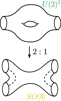
Figure 12: The G-curve of the $SU(2)\times SU(2)$ gauge theory coupled by two bifundamentals is a double cover over the G-curve of the $SO(4)$ gauge theory coupled to four hypers.

Let us again interpret the $\mathbb{Z}_{2}$ twist-lines as branch-cuts. As illustrated in Figure 12, this time the branched double cover of the G-curve is a torus with two punctures. The punctures on the torus project to two of the four branch-points of the double covering, which means that there must be a $SU(2)$-flavor symmetry attached to them. This is precisely the the same structure as that of the Gaiotto curve of the $SU(2)\times SU(2)$ gauge theory coupled to two bifundamentals.

However, note that the $SU(2)\times SU(2)$ G-curve has two complex structure parameters corresponding to the two marginal couplings $q_{U(2),1}$ and $q_{U(2),2}$, whereas the $SO(4)$ G-curve has only a single complex structure parameter corresponding to the marginal coupling $q_{SO(4)}$ of the $SO(4)$ theory. The $\mathbb{Z}_{2}$-symmetry on the cover curve implies that we should identify $q_{U(2)}=q_{U(2),1}=q_{U(2),2}$ in order to relate the $SU(2)\times SU(2)$ Gaiotto curve to the $SO(4)$ Gaiotto curve.

In equation (28) we found that the relation between the marginal couplings of the $SO(4)$ and the $SU(2)\times SU(2)$-theory is given by the modular lambda mapping

$$\boxed{q_{SO(4)}=\lambda(2\tau_{U(2)})\,.}$$ (47)

The above covering relation between their Gaiotto curve explains the appearing of this lambda mapping geometrically, as it relates the complex structure parameter of the torus to the complex structure parameter of the four-punctured sphere, when we identify $\tilde{q}_{SO(4)}=q_{SO(4)}$.

Mainly for future convenience, let us make the covering map explicitly. Take a torus $T^{2}$ with half-periods $\omega_{1}$ and $\omega_{2}$ and consider the map $T^{2}\to\mathbb{C}\mathbb{P}^{2}$ given by

$$(\wp(z):\wp^{\prime}(z):1),$$

where $\wp(z)$ is the Weierstrass $\wp$-function. Since the Weierstrass $\wp$-function satisfies

$$\wp^{\prime}(z)^{2}=4\wp(z)^{3}-g_{2}\wp(z)-g_{3},$$

it defines a branched double cover over the sphere $\mathbb{P}^{1}$. The branch points are determined by the zeroes and poles $\{0,\omega_{1},\omega_{2},\omega_{3}=\omega_{1}+\omega_{2}\}$ of the derivative $\wp^{\prime}(z)$ of the Weierstrass $\wp$-function. The double covering is thus given by the equation

$$t^{2}=4(s-e_{1})(s-e_{2})(s-e_{3})$$

with $e_{i}=\wp(\omega_{i})$. The points $\omega_{3}=\tau$ and $2\tau$ on the torus $T^{2}$ map onto the two branch points $e_{3}$ and $\infty$ on the sphere $\mathbb{P}^{1}$. Let us call $q_{SO(4)}$ the cross-ratio of the four branch points $0,e_{1},e_{2},e_{3}$. By the shift $s\mapsto s+\frac{(1+q_{SO(4)})}{3}$ we simply bring the curve into the form

$$t^{2}=4s(s-1)(s-q_{SO(4)}).$$

The mapping between the $SU(2)\times SU(2)$ Gaiotto curve and the $SO(4)$ Gaiotto curve is thus a combination of the Weierstrass map $\wp$ and a simple Möbius transformation. This indeed determines (47) as the mapping between the respective complex structure parameters.

4 Conformal blocks and ${\cal W}$-algebras

Compactifying the six-dimensional superconformal $(2,0)$ theory of type $ADE$ on either a two-dimensional Riemann surface or a four-manifold, suggests that there should be a correspondence between the following two systems. The first system is a four-dimensional superconformal ${\cal N}=2$ gauge theory with $ADE$ gauge group and whose Gaiotto curve is equal to the Riemann surface. The second system is a two-dimensional field theory that lives on the Riemann surface and should be characterized by an $ADE$ type.

Remember that the tubes of the Gaiotto curve are associated to the ADE gauge group of the ${\cal N}=2$ gauge theory, and the punctures on the G-curve to matter. Decomposing the G-curve into pairs of pants suggests that the marginal gauge couplings $\tau_{\rm UV}$ should be identified with the sewing parameters $q=\exp(2\pi i\tau_{\rm UV})$ of the curve. The symmetry of the two-dimensional theory should be related to the ADE gauge group. Furthermore, two-dimensional operators that are inserted at punctures of the G-curve should encode the flavor symmetries of the corresponding matter multiplets.

A particular instance of such a 4d–2d connection was discovered in [2]. It was found that instanton partition functions in the $\Omega$-background $\mathbb{R}^{4}_{\epsilon_{1},\epsilon_{2}}$ for linear and cyclic $U(2)$ quiver gauge theories are closely related to Virasoro conformal blocks of the pair of pants decomposition of the corresponding G-curves. In this so-called AGT correspondence the central charge of the Virasoro algebra is determined by the value of the two deformation parameters $\epsilon_{1}$ and $\epsilon_{2}$ as

$$c =1+\frac{6(\epsilon_{1}+\epsilon_{2})^{2}}{\epsilon_{1}\epsilon_{2}}.$$ (48)

The conformal weights of the vertex operators at the punctures of the G-curve are specified by the masses of the hypermultiplets in the quiver theory, and the conformal weights of the fields in the internal channels are related in the same way to the Coulomb branch parameters.

Figure 13: The AGT correspondence relates the instanton partition function of the $U(2)$ gauge theory coupled to four hypermultiplets to a Virasoro conformal blocks on the four-punctured sphere with vertex operator insertions at the four punctures.

More precisely, the instanton partition function can be written as the product of the Virasoro conformal block times a factor that resembles a $U(1)$ partition function. The interpretation for this is that the single Casimir of degree 2 of the subgroup $SU(2)\subset U(2)$ corresponds to the energy-stress tensor of the CFT, and the overall $U(1)$ factorizes. This picture was made more explicit in [20].

For general gauge groups with more Casimirs we expect the CFT to have a bigger symmetry group. Since the symmetries of a CFT are captured by its so-called ${\cal W}$ or chiral algebra, we expect that the Nekrasov partition functions should be identified with ${\cal W}$-blocks instead of Virasoro blocks. For $SU(N)$, this picture was proposed and checked in [15]. The relation between Hitchin systems and ${\cal W}$-algebras was also discussed in [50]. Before continuing let us first introduce ${\cal W}$-algebras and some other concepts in CFT.

4.1 ${\cal W}$-algebras, chiral blocks and twisted representations

The concept of a conformal block can be generalized for theories with bigger symmetry groups. The symmetries of a two-dimensional conformal field theory are given by its ${\cal W}$ (or chiral) algebra. The algebra ${\cal W}$ always contains the energy-stress tensor $T$, a distinguished copy of the Virasoro algebra describing the behavior under conformal coordinate transformations. The fields of the theory decompose into highest weight representations of the ${\cal W}$-algebra. For an introduction to ${\cal W}$ algebras, see [51].

There is no complete classification all ${\cal W}$ algebras, but many examples are known and have been studied. One particular family of examples are the the so-called Casimir algebras, which are based on simply laced Lie algebras. Its generators are constructed from the $\mathfrak{g}$-invariant contractions of the current field $J(z)$ of the affine Lie algebra $\mathfrak{g}$. The series of ${\cal W}_{N}$-algebras, for instance, is related to the $A_{N}$ Lie algebras. In [15] ${\cal W}_{N}$-blocks have been related to the instanton partition functions corresponding to $U(N)$ gauge theories. It is natural to expect that also the other Casimir algebras appear as dual descriptions of instanton counting.

Since the spectrum of the CFT decomposes into representations of the ${\cal W}$ algebra, we can use generalized Ward identities to relate correlation functions of (${\cal W}$-)descendant fields to correlation functions of (${\cal W}$-)primary fields. In the case of the Virasoro algebra, we can always reduce them to functions of primary fields only. For general ${\cal W}$-algebras this is only possible if one restricts to primary fields on which the ${\cal W}$-fields satisfy additional null relations.

We can make use of this property by computing chiral blocks. For a given configuration of a punctured Riemann surface, we define the chiral block by picking a representation $\phi$ for every tube, inserting the projector on the representation $P_{{\cal H}_{\phi}}$ at that point in the correlator, and dividing by the product of all three point functions of the primary fields. By the above remarks the result is then independent of the three-point functions of the theory, i.e. it only depends on the kinematics of the theory.

In the simplest configuration, the sphere with four punctures, the chiral block is thus given by

$${\cal F}=\frac{\langle V_{1}(\infty)V_{2}(1)P_{{\cal H}_{\phi}}V_{3}(q)V_{4}(0)\rangle}{\langle V_{1}(\infty)V_{2}(1)|\phi\rangle\langle\phi|V_{3}(1)V_{4}(0)\rangle}\ .$$ (49)

Note that this definition differs slightly from the usual definition, as we have not divided out a factor $q^{h_{\phi}-h_{3}-h_{4}}$. Our definition will be slightly more convenient to work with. On the gauge theory side it corresponds to the partition function including the perturbative contribution. Also, let us take the convention in what follows that whenever we write a correlator, we assume that it is divided by the appropriate primary three point functions. The projector is usually written as

$$P_{{\cal H}_{\phi}}=\sum_{I,J}|\phi_{I}\rangle\langle\phi_{J}|(K^{-1})_{I,J}$$ (50)

where $I=(i_{1},i_{2},\ldots)$ denotes the ${\cal W}$ descendants, such that $\phi_{I}=W_{-i_{1}}W_{-i_{2}}\cdots\phi$ is a ${\cal W}$ descendant. $K$ is the inner product matrix and the sum runs over all ${\cal W}$ descendants of $\phi$.

A representation $\phi$ of ${\cal W}$ is called untwisted if it is local with respect to ${\cal W}$, so that one can freely move ${\cal W}$-fields around it. The ${\cal W}$-fields then have integer mode representations around that representation.

More generally, the ${\cal W}$-fields can pick up phases when circling around $\phi$, so that the correlation function has a branch cut extending from $\phi$. Such $\phi$ are called twisted representations. Because of the phase $\alpha$ picked up by the ${\cal W}$-fields, their modes are no longer integer, but given by $r\in\mathbb{Z}+\alpha$.

A particular case of twisted representations can appear when the ${\cal W}$ has an outer automorphism such as a $\mathbb{Z}_{N}$-symmetry. Let us say that by circling around a twisted representation the algebra ${\cal W}$ gets mapped to an image under $\mathbb{Z}_{N}$, such as

$$W_{k}\mapsto W_{k+1}\ ,\qquad k=1,\ldots N\ .$$ (51)

By choosing linear combinations $W^{(k)}$ of the modes $W_{k}$ that are eigenvectors under the automorphisms, the $W^{(k)}$ indeed pick up phases $2\pi ik/N$. For $N=2$, the case that we are interested in below, the ${\cal W}$-algebra thus decomposes into generators $W^{+},W^{-}$ of integer and half-integer modes respectively.

Let us finally note that in the case of Liouville theory the ${\cal W}$-algebra is simply the Virasoro algebra. Example of conformal field theories with bigger ${\cal W}$-algebras are Toda theories.

4.2 The $SO(4)$ and $Sp(1)$ AGT correspondence

Remember that the ${\cal N}=2$ geometry is characterized by a ramified Hitchin system on the Gaiotto curve. For conformal $SO(2N)$ and $Sp(N-1)$ gauge theories the Hitchin system is described in terms of the differentials $\phi_{2k}$ (for $k=1,\ldots,N-1$) and $\tilde{\phi}_{N}$ that can be constructed out of the $D_{N}$-invariants ${\rm Tr}\left(\Phi^{2k}\right)$ and $\textrm{Pfaff}(\Phi)$, respectively. In the six-dimensional $(2,0)$ theory these differentials appear as a set of chiral operators whose conformal weights are equal to the exponents of the Lie algebra. When we reduce the six-dimensional theory over a four-manifold we expect these operators to turn into the Casimir operators ${\cal W}^{(2k)}$ and $\tilde{\cal W}^{(N)}$ of the ${\cal W}(D_{N})$-algebra. The $\mathbb{Z}_{2}$-automorphism of the $D_{N}$-algebra translates to an additional $\mathbb{Z}_{2}$-symmetry on the level of the CFT, and we thus expect a relation to a twisted ${\cal W}(D_{N})$-algebra. In other words, we expect that the Lie algebra underlying the Hitchin system is precisely reflected in the Casimir operators of the corresponding ${\cal W}$-algebra on the Gaiotto curve.

Let us now put all the pieces together and formulate the AGT correspondence for $SO(4)$ and $Sp(1)$. Since the definition of the Gaiotto curve for both theories involves the $SO(4)$-invariants $\phi_{2}$ and $\tilde{\phi}_{2}$ of degree two, we expect this CFT to have an underlying ${\cal W}(D_{2})$-algebra. We will denote this algebra by ${\cal W}(2,2)$, as it contains two Casimir operators of weight two. In fact those operators correspond to two copies $T^{A}$ and $T^{B}$ of the Virasoro algebra.

Similar to the correspondence between $U(2)$ instanton partition function and Virasoro conformal blocks, the new correspondence is between $SO(4)/Sp(1)$ instanton partition functions and twisted ${\cal W}(2,2)$-algebra blocks. The configuration of the block is given in the following way: At the full punctures of the $SO(4)/Sp(1)$ G-curve insert untwisted vertex operators, whose weights correspond to the masses of the $Sp(1)$ fundamental hypers. At the half punctures, insert twisted vertex operators. Whenever a half-puncture lifts to a regular point on the cover, we should insert the vacuum of the twist sector $\sigma$, which we will describe later on. For any half-puncture that lifts to a puncture on the cover we may insert a general twisted field, whose single weight corresponds to the mass of the $SO(4)$ fundamental hyper.

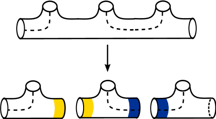
Figure 14: Twisted ${\cal W}(2,2)$-algebra blocks can be computed by decomposing the Riemann surface into pairs of pants. Internal tubes that have a $\mathbb{Z}_{2}$ twist line (blue) correspond to an $Sp(1)$ gauge group and carry twisted representations of ${\cal W}(2,2)$. Internal tubes without a twist line (yellow) correspond to $SO(4)$ and carry two copies of the Virasoro algebra.

When decomposing the Gaiotto curve into pair of pants, we cut tubes with or without twist lines (see Figure 14). A tube with a twist line corresponds to a $Sp(1)$ gauge group, and the weight of the twisted primary in the channel corresponds to its single Coulomb branch parameter $a$. A tube without a twist line corresponds to a $SO(4)$ gauge group, and the two weights of the untwisted primary in the channel correspond to the two Coulomb branch parameters $a_{1}$ and $a_{2}$. All of this is summarized in table 1.

   N=2 gauge theory CFT

   $$SO(4)/Sp(1)$$ quiver Gaiotto curve

    fund. hyper untwisted representation

    fund. hyper twisted representation

    bifund. hyper twist vacuum

    Coulomb par. weight of twisted int. channel

    Coulomb pars. weights of untwisted int. channel

Table 1: The AGT correspondence for $SO(4)/Sp(1)$.

The detailed identification of parameters can be found in the examples we will work out. These examples will show that $Sp(1)/SO(4)$ instanton partition functions agree with the twisted ${\cal W}(2,2)$ up to a spurious factor that is independent of the Coulomb and mass parameters of the gauge theory. Note in particular that, unlike in the original $U(2)$ case, no $U(1)$ prefactor appears, which is exactly what one would expect.

We can also use this correspondence to explain the relation between $Sp(1)/SO(4)$ and $U(2)$ theories. More precisely, given an $Sp(1)/SO(4)$ Gaiotto curve, we first map the corresponding chiral block to its double cover. This is in fact a well-known method to compute twisted correlators. The resulting configuration can then be mapped to a $U(2)$ configuration by a suitable conformal coordinate transformation. We will argue below that such a coordinate transformation only introduces a spurious factor. It thus follows that the partition function of the $U(2)$ configuration agrees up to a spurious factor with the partition function of the $Sp(1)/SO(4)$ configuration once expressed in terms of the same coupling constants. To put it another way, the difference between $U(2)$ and $Sp(1)/SO(4)$ partition functions is indeed only a reparametrization of the moduli space caused by choosing a different renormalization scheme.

4.3 Correlators for the ${\cal W}(2,2)$ algebra and the cover trick

As mentioned above, the algebra ${\cal W}(2,2)$ contains two Casimir operators of weight two. These operators can be identified with two Virasoro tensors $T^{A}(z)$ and $T^{B}(z)$. The ${\cal W}$-algebra thus decomposes into two copies of the Virasoro algebra. This reflects the decomposition of the Lie algebra $\mathfrak{so}(4)\cong\mathfrak{su}(2)_{A}\times\mathfrak{su}(2)_{B}$. Geometrically, the fact that we find two copies of the Virasoro algebra follows simply from the double covering that relates the $U(2)$ and the $Sp(1)/SO(4)$ Gaiotto curves. A single copy of the Virasoro algebra associated to the cover $U(2)$ Gaiotto curve descends to two copies of the Virasoro algebra on the base $Sp(1)/SO(4)$ Gaiotto curve.

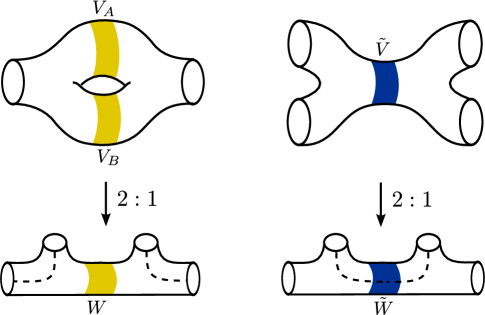
Figure 15: On the left (right): Illustration of the branched double covering of the $SU(2)$ G-curve over the $SO(4)$ G-curve ($Sp(1)$ G-curve). The yellow (blue) tubular neighborhoods $W$ and $\tilde{W}$ on the base curves are part of internal tubes without (with) a $\mathbb{Z}_{2}$ twist line. On the cover the yellow (blue) patches illustrate their respective inverse images. The ${\cal W}$-algebra modes associated to both base tubes lift to a single copy of the Virasoro algebra on their inverse images.

As illustrated on the left in Figure 15, this is in particular the case for an internal tubular neighborhood of the $SO(4)$ Gaiotto curve. The single copy of the Virasoro algebra on its inverse image descends to two copies of the Virasoro algebra on the tubular neighborhood itself. The $SO(4)/Sp(1)$ Gaiotto curves additionally contain $\mathbb{Z}_{2}$ twist-lines. When crossing such a twist-line the two copies of the Virasoro algebra get interchanged. We thus propose an underlying twisted ${\cal W}(2,2)$-algebra. The actual energy-stress tensor $T^{+}(z)=T^{A}(z)+T^{B}(z)$ is of course invariant, whereas $T^{-}(z)=T^{A}(z)-T^{B}(z)$ picks up a minus sign.

To compute the corresponding chiral blocks, we decompose the Gaiotto curves into pair of pants and sum over all ${\cal W}$-descendants of a given channel. The only difference with Virasoro correlators is that there are now two types of tubes to cut, those with $\mathbb{Z}_{2}$ twist-lines and those without. This is illustrated in Figure 14.

When cutting open a tube without a $\mathbb{Z}_{2}$ twist-line, the intermediate fields are given by $L^{A}$ and $L^{B}$-descendants of an untwisted representation, characterized by the conformal weights $(D_{A},D_{B})$ under $L^{A}_{0}$ and $L^{B}_{0}$. We can therefore associate the Hilbert space

$${\cal H}_{SO(4)}=\{L^{A}_{-m_{1}}\cdots|\phi_{A}\rangle\otimes L^{B}_{-n_{1}}\cdots|\phi_{B}\rangle\ :m_{i}\in\mathbb{N},n_{i}\in\mathbb{N}\},$$ (52)

where $|\phi_{A/B}\rangle$ has weight $D_{A/B}$, to a tube without a $\mathbb{Z}_{2}$ twist-line. On the other hand, if we cut a tube with a $\mathbb{Z}_{2}$ twist-line, the intermediate fields are in a twisted representation of the ${\cal W}$-algebra. It is then most convenient to describe them in terms of descendants of $L^{+}$ and $L^{-}$,

$${\cal H}_{\widetilde{Sp}(1)}=\{L^{+}_{-m_{1}}\cdots L^{-}_{-r_{1}}\cdots|\phi_{C}\rangle\ :m_{i}\in\mathbb{N},r_{i}\in\frac{1}{2}+\mathbb{N}\}\ .$$ (53)

Note that since $L^{-}$ has no zero mode, the representation $\phi_{C}$ is characterized by just a single weight.

To actually compute three point functions with twist fields, we can use the well-known cover trick, which is nicely explained in e.g. [52, 53] : We find a function that maps the punctured Riemann surface with branch cuts to a cover surface which does not have any branch cuts. Since the theory is conformal, we know how the correlation functions transform under this map. On the cover we can then evaluate a correlation function with no twisted fields and no branch cuts in the usual way. In order for this to work, we need to find a cover map that has branch points where the twist fields are inserted. The precise map from the base to the cover thus depends on the positions of the branch cuts. On the cover there is then only a single copy of the Virasoro algebra.

To illustrate all of this, let us take the following simple model as a map from the cover to the base:

$$\tilde{z}\mapsto z=\tilde{z}^{2}\ .$$ (54)

This particular map has branch cuts at 0 and $\infty$, and is thus suitable to deal with correlation functions that have twist fields at those two points. We can relate the stress-energy tensor on the cover $T(\tilde{z})$ to the two copies on the base in the following manner. The stress-energy tensor on the cover transforms to

$$T(\tilde{z})=\left(\frac{d\tilde{z}}{dz}\right)^{-2}\left[T(z)-\frac{c}{12}\{\tilde{z};z\}\right]\ ,$$ (55)

where the Schwarzian derivative given by

$$\{\tilde{z};z\}=\frac{\tilde{z}^{\prime\prime\prime}}{\tilde{z}}-\frac{3}{2}\left(\frac{\tilde{z}^{\prime\prime}}{\tilde{z}^{\prime}}\right)^{2}\$$ (56)

appears because $T$ is not a primary field. Around the branch point 0 on the base we can then define two ${\cal W}$-fields $T^{+}$ and $T^{-}$ by picking out the even and odd modes of $T$,

$$L^{+}_{n} = 2\oint\frac{dz}{z^{n-1}}T(z)=\frac{1}{2}L_{2n}+\frac{3c}{48}\delta_{n,0}\qquad(\mathrm{for}\,n\in\mathbb{Z}),$$ (57)

$$L^{-}_{r} = 2\oint\frac{dz}{z^{r-1}}T(z)=\frac{1}{2}L_{2r}\qquad(\mathrm{for}\,r\in\frac{1}{2}+\mathbb{Z}).$$ (58)

The $L^{+}$ then form a Virasoro algebra with central charge $2c$, and $T^{-}$ is a primary field of weight 2. As discussed above, the twisted field $\phi$ at the point 0 is a twisted representation of $T^{-}$ and $T^{+}$ which has only one weight, namely the eigenvalue of $L^{+}_{0}$. This means that on the cover point there sits a field $\phi$ which is an untwisted representation of the Virasoro algebra of the corresponding weight, and its $L^{+}$ and $L^{-}$ descendants are given by even and odd $L$ descendants.

There is one special twist field $\sigma$ which has the property that its lift to the cover gives the vacuum. It has the lowest possible conformal weight for a twist field and serves in some sense as the vacuum of this particular twist sector.

Around any other puncture on the base that is not a branch point, we simply obtain two independent copies $L^{A}$ and $L^{B}$ of the Virasoro algebra, coming from the two pre-images of the punctures on the cover. As long as we stay away from branch points, the Virasoro tensor $T(\tilde{z})$ on the cover is given by $T^{A}(\tilde{z})$ on the first and by $T^{B}(\tilde{z})$ on the second sheet of the cover. Since $T^{A}$ and $T^{B}$ commute on the base, a field $\phi^{A,B}$ on the base factorizes into representations of $T^{A}$ and $T^{B}$, $\phi^{A,B}=\phi^{A}\otimes\phi^{B}$ with conformal weights $(D_{A},D_{B})$ under both copies. On the cover this leads to two untwisted fields $\phi^{A}$ and $\phi^{B}$ sitting at the two images of the cover map, both of which are again untwisted representations of the Virasoro algebra.

Let us now to turn to some more technical points. The map from the base to the cover in general introduces corrections to the three point functions. In particular since one or more of those fields are descendants, they will exhibit more complicated transformation properties than we are used to from primary fields. Let us therefore briefly discuss how conformal blocks behave under coordinate transformations.

When dealing with descendants fields, it will be useful to use the notation $\phi(z)=V(\phi,z)$, which we shorten to $V_{i}(z)$ if $\phi_{i}(z)$ is a primary field. The transformation of a general descendant field $\phi$ under a general coordinate transformation $z\mapsto f(z)$ is given by [54]

$$D_{f}V(\phi,z)D_{f}^{-1}=V\left(f^{\prime}(z)^{L_{0}}\prod_{n=1}^{\infty}e^{T_{n}(z)L_{n}}\phi,f(z)\right),$$ (59)

where the operator $D_{f}$ is given by

$$D_{f}=e^{f(0)L_{-1}}f^{\prime}(0)^{L_{0}}\prod_{n=1}^{\infty}e^{T(0)_{n}L_{n}}\ .$$ (60)

Here we take all products to go from left to right. The functions $T_{n}(z)$ are defined recursively. The first two are given by

$$T_{1}(z)=\frac{f^{\prime\prime}(z)}{2f^{\prime}(z)}\ ,\qquad T_{2}(z)=\frac{1}{3!}\left(\frac{f^{\prime\prime\prime}(z)}{f^{\prime}(z)}-\frac{3}{2}\left(\frac{f^{\prime\prime}(z)}{f^{\prime}(z)}\right)^{2}\right)\ .$$ (61)

First note that if $\phi$ is a primary field, (59) reduces to the standard expression $\phi\mapsto(f^{\prime}(z))^{h}\phi$. For general descendants however, the result will be a linear combination of correlators of lower descendant fields. Also note that $T_{2}(z)$ is in fact a multiple of the Schwarzian derivative. It is actually true that all higher $T_{n}(z)$ are sums of products of derivatives of the Schwarzian derivative. Since the Schwarzian derivative of a Möbius transformation vanishes, those transformations lead to much simpler expressions.

In some cases however we can avoid having to transform descendant fields. Assume that we want to compute the chiral block of a configuration for which we know the base to cover map $f$. When we go to the cover, we can use the fact that $D_{f}$ is a function of the Virasoro modes $L_{n}$ only. This means that it does not mix different representations, so that, more formally,

$$D_{f}^{-1}P_{{\cal H}_{\phi}}D_{f}=P_{{\cal H}_{\phi}}\ .$$ (62)

From this it follows that conformal block has the same transformation properties as the underlying correlation function, as can be seen e.g. in the simplest case

$$\langle V_{1}(z_{1})V_{2}(z_{2})P_{{\cal H}_{\phi}}V_{3}(z_{3})V_{4}(z_{4})\rangle$$ (63)

$$\qquad=\prod_{i=1}^{4}(f(z_{i}))^{h_{i}}\langle V_{1}(f(z_{1}))V_{2}(f(z_{2}))P_{{\cal H}_{\phi}}V_{3}(f(z_{3}))V_{4}(f(z_{4}))\rangle\ .$$

Note that what we have said here is strictly speaking true only for global coordinate transformations $f$, i.e. for Möbius transformations

$$z\mapsto\gamma(z)=\frac{az+b}{cz+d}\ ,\qquad a,b,c,d\in\mathbb{C}\ .$$ (64)

Other transformations, in particular also cover maps, must be treated with more caution, as they can introduce new singularities. On a technical level this means that at some points $f$ is no longer locally invertible and $D_{f}$ does no longer annihilate the vacuum.

From these remarks it follows that conformal blocks exhibit the same behavior as correlation functions under coordinate transformations. This does not mean, however, that their behavior under channel crossing is the same. In particular, the full partition function must be crossing symmetric, whereas individual conformal blocks will transform into each others in a very complicated manner. More precisely, if we expand the analytic continuation of the full partition function around 0 or $\infty$, then the resulting power series has essentially the same form as the original expansion. This is simply a consequence of covariance under Möbius transformations and the fact that we can change the order of operators in the correlation function, as they are mutually local. In contrast, even though the conformal block still transforms nicely under coordinate changes, the projector in it is not local, so that we cannot change the order of the fields at will, which means that expansions around different points will look different.

Coming back to the computation of the conformal block, if we do not know the full cover map, then we need to decompose the conformal block into three point functions with twist fields. We then evaluate these three point functions by mapping them to their appropriate covers. Note that in that case the cover maps are different for the individual three point functions, and no longer defined for the entire configuration. This means that the above arguments no longer apply, and that we must take into account the transformation properties of the descendant fields.

Let us make one more remark concerning prefactors in the AGT correspondence. From (63) we see that any coordinate transformation on the G-curve leads to a product of prefactors of the form $(f^{\prime})^{h}$. From the way $h$ is related to the gauge theory masses, it follows that this factor does not depend on the Coulomb branch parameters, and that it only contributes to ${\cal F}_{0}$ and ${\cal F}_{1}$. Nevertheless the structure of the exponent of the $U(1)$ prefactor found in [2] is different, so that it cannot be transformed away in this way, which is in line with what was expected on physical grounds.

4.4 Examples

We proceed to verify the correspondence in detail in a few examples, the $Sp(1)$ gauge theory coupled to four hypermultiplets and the $SO(4)$ gauge theory coupled to two hypermultiplets.

4.4.1 $Sp(1)$ versus $U(2)$ correlators

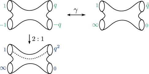
Figure 16: On the left, the G-curve of the $Sp(1)$ gauge theory coupled to 4 hypers and its double cover. The Möbius transformation $\gamma$ relates the double cover to the $SU(2)$ G-curve.

Recall that the G-curve for the $Sp(1)$ gauge theory coupled to four massive hypers is given by a four-punctured sphere, as illustrated on the bottom left of Figure 16. The two half-punctures at 1 and $q^{2}$ are connected by a branch cut. As we have found in section 3, the cross-ratio $q^{2}$ of the four punctures can be expressed in terms of the $Sp(1)$ instanton coupling $q_{Sp(1)}$ as

$$q^{2}=\left(\frac{q_{Sp(1)}}{4}\right)^{2}.$$ (65)

The chiral block we need to evaluate is obtained by cutting the tube with the twist line, so that

$${\cal F}_{Sp(1)}(q)=\langle V_{1}^{A,B}(\infty)\sigma(1)P_{{\cal H}_{\phi}}\sigma(q^{2})V_{2}^{A,B}(0)\rangle$$ (66)

where the vertex operators $V^{A,B}_{1,2}$ factorize into representations of $T^{A}$ and $T^{B}$ of weight $(h_{1},h_{2})$ and $(h_{3},h_{4})$,

$$V_{1}^{A,B} =V_{1}^{A}V_{1}^{B}$$

$$V_{2}^{A,B} =V_{2}^{A}V_{2}^{B}.$$

Here we identified the half-integral mode $L_{-\frac{1}{2}}^{-}$ of the twisted ${\cal W}(2,2)$ algebra with the one-instanton modulus $q_{Sp(1)}$ of the $Sp(1)$ theory.

To evaluate the correlator with twist fields, we want to go to the double cover. The base has half-punctures at $1$ and $q^{2}$, so that we map it to the double cover by

$$z\mapsto\tilde{z}=\pm\sqrt{\frac{z-q^{2}}{z-1}}\ .$$ (67)

This maps has indeed branch points at 1 and $q^{2}$, and it maps the fields at 0 and $\infty$ to $\pm q$ and $\pm 1$. The block (66) on the base thus becomes the block on the cover (up to some constant prefactor)

$${\cal F}_{Sp(1)}(q)=\left(1-q^{2}\right)^{\sum_{i}h_{i}}\langle V^{B}_{1}(-1)V^{A}_{1}(1)P_{{\cal H}_{\phi}}V^{A}_{2}(q)V^{B}_{2}(q)\rangle_{C}\ .$$ (68)

Note that since we know the full base-cover map, we were able to make use of (63) without worrying about descendant fields. To evaluate (68), we write it as a sum over three point functions in the usual manner. Let us therefore define three point coefficients on the cover by

$$\mathbf{\tilde{C}}^{h_{1},h_{2};h_{3}}_{I_{1},I_{2},I_{3}}=\langle V^{1}_{I_{1}}(1)V^{2}_{I_{2}}(-1)V^{3}_{I_{3}}(0)\rangle$$

where $I_{i}$ gives the Virasoro descendants acting on $V^{i}$, which we will usually denote by Young diagrams. The conformal block can then be evaluated as

$${\cal F}_{Sp(1)}(q)=\left(1-q^{2}\right)^{\sum_{i}h_{i}}\sum_{I_{a},J_{a}}\mathbf{\tilde{C}}^{h_{1},h_{2};h_{a}}_{\bullet,\bullet,I_{a}}\mathbf{\tilde{C}}^{h_{3},h_{4};h_{a}}_{\bullet,\bullet,J_{a}}(\langle V^{a}_{I_{a}}|V^{a}_{J_{a}}\rangle)^{-1}q^{h_{a}+|I_{a}|}\\ =q^{h_{a}}\left(1+\frac{2(h_{1}-h_{2})(h_{3}-h_{4})}{h_{a}}q+\ldots\right)\ .$$ (69)

Using the identification of parameters

$$h_{i} =\frac{1}{\epsilon_{1}\epsilon_{2}}\left(\frac{Q^{2}}{4}-m_{i}^{2}\right),$$

$$h_{a} =\frac{1}{\epsilon_{1}\epsilon_{2}}\left(\frac{Q^{2}}{4}-a^{2}\right),$$

where $Q=\epsilon_{1}+\epsilon_{2}$ and the momenta $m_{i}$ are related to the mass parameters $\mu_{i}$ as

$$\begin{array}[]{lll}m_{1}=\frac{\mu_{1}+\mu_{2}}{2}&&m_{3}=\frac{\mu_{3}+\mu_{4}}{2}\\ m_{2}=\frac{\mu_{1}-\mu_{2}}{2}&&m_{4}=\frac{\mu_{3}-\mu_{4}}{2},\end{array}$$

we find that equation (68) is indeed equal to the $Sp(1)$ instanton partition function up to a spurious factor independent of $a$ and $\mu_{i}$,

$$Z^{Sp(1)}(q_{Sp(1)})=\left(1-\left(\frac{q_{Sp(1)}}{4}\right)^{2}\right)^{-\frac{1}{16}(c+1)}{\cal F}_{Sp(1)}(q_{Sp(1)})\ .$$ (70)

Note in particular that this spurious factor is independent of the masses of the hypermultiplets, in contrast to the spurious factor in the AGT correspondence for unitary gauge groups. This is indeed as expected, as the latter should come from the decoupled $U(1)$ in the $U(2)$, whereas there is no such $U(1)$ in the $Sp(1)$ setup. This fact will also be important for extending the $Sp(1)$-correspondence to linear $Sp(1)-SO(4)$ quivers.

Relation to the $U(2)$ correlator

We already knew that the full $Sp(1)$ and $U(2)$ Nekrasov partition function are related by the change of parameters (65). To understand this better from the conformal field theory perspective, let us study the relation between the $Sp(1)$ conformal block (66) and the $U(2)$ conformal block.

We have used the fact that the conformal block on the base (66) can be related to the block on the cover (68). The block on the cover is obviously very closely related to the original $U(2)$ configuration depicted on the right of Figure 11. We can map one to the other using the Möbius transformation $\gamma$ given by equation (44). This is of course only possible provided that we make their cross ratios agree by identifying

$$q_{U(2)}=\frac{q_{Sp(1)}}{\left(1+\frac{q_{Sp(1)}}{4}\right)^{2}}\ ,$$

which is exactly the relation found on the gauge theory side.

From equation (63) we also know that this transformation only introduces an overall prefactor which does not depend on the weight of the intermediate channel, so that it is an $a$-independent prefactor. If we were interested in the relation between instanton partition functions without the perturbative part, we would need to divide both (68) and the $U(2)$ block by $q^{h_{a}-h_{1}-h_{4}}$. The $a$-dependent part of the ratio of the two is then

$$\left(\frac{q_{U(2)}}{q_{Sp(1)}}\right)^{h_{a}}.$$

On the gauge theory side, this factor originates from the difference in the instanton part of $F_{0}$. By construction, $F_{0}^{\rm inst}-\tilde{F}_{0}^{\rm inst}=-a^{2}(\log q_{U(2)}-\log q_{Sp(1)})$, which agrees with the above factor (for $Q=0$).

4.4.2 $SO(4)$ versus $U(2)\times U(2)$ correlators

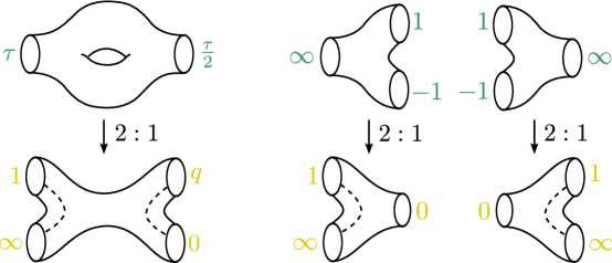
Figure 17: The G-curve for the $SO(4)$ coupled to two hypermultiplets and its double cover. The left picture illustrates the global mapping between the $SO(4)$ G-curve and its double cover, whereas the right picture illustrates the local mappings that we use to compute the twisted ${\cal W}(2,2)$ conformal block on the $SO(4)$ G-curve.

Let us now turn to the $SO(4)$ case. The G-curve for the $SO(4)$ theory with two hypers in the fundamental is given in the lower left of Figure 17. The chiral block we need to evaluate is

$${\cal F}_{SO(4)}(q_{SO(4)})=\langle\hat{V}_{1}(\infty)\sigma(1)P_{{\cal H}_{\phi}}\sigma(q_{SO(4)})\hat{V}_{2}(0)\rangle\ .$$ (71)

Note that we identified the integral modes $L^{A/B}_{-1}$ with the one-instanton parameter $q_{SO(4)}$.

Similarly to the $Sp(1)$ example that we discussed previously, there is an elegant way of obtaining the chiral block that makes use of the fact that we know the double cover map of the full configuration (71). This double covering was described in section 3.2.2. In particular it maps the punctures

$$(\infty,1,q_{SO(4)},0)\mapsto(1/2,0,\tau/2,(1+\tau)/2)\ .$$

The configuration on the cover is a torus with two punctures at 0 and $q_{U(2)}$. The conformal block for this configuration has been computed in [2] and agrees with the $U(2)\times U(2)$ instanton partition function. Up to spurious prefactors introduced by the mapping to the cover, (71) is thus given by the conformal block of the two punctured torus expressed in terms of $q_{SO(4)}$.

However, in more general examples (i.e. the ones that we encounter in section 5) it will be much harder to find the global mapping between the $SO/Sp$ Gaiotto curve and its double cover. We thus need to develop a method that doesn’t require this global information, and computes the twisted ${\cal W}(2,2)$ block from a simple decomposition of the Gaiotto curve into pairs of pants. Let us exemplify this for the $SO(4)$ Gaiotto curve.

Evaluating the $SO(4)$-block (71) is more complicated than the $Sp(1)$-block we considered previously. Since it has two branch cuts, there is no longer a simple square root map that maps the block (71) to its double cover, the torus. What we will do instead is to first decompose the block into three point functions, and then map those three point functions individually to their covers, as depicted on the right side of Figure 17.

Let us also define twisted three point coefficients on the base as

$$\mathbf{C}^{h_{A},h_{B};h_{1}}_{I_{A},I_{B},\bullet}:=\langle\hat{V}_{1}(\infty)\sigma(1)V^{A,B}_{I_{A},I_{B}}(0)\rangle,$$ (72)

so that

$${\cal F}_{SO(4)}(q_{SO(4)})=\sum_{I_{A},J_{A},I_{B},J_{B}}\mathbf{C}^{h_{A},h_{B};h_{1}}_{I_{A},I_{B},\bullet}\mathbf{C}^{h_{A},h_{B};h_{2}}_{J_{A},J_{B},\bullet}(\langle V^{2,3}_{I_{A},I_{B}}|V^{2,3}_{J_{A},J_{B}}\rangle)^{-1}q_{SO(4)}^{h_{A}+|I_{A}|+h_{B}+|I_{B}|}\ .$$

Note that we have used that $\sigma(1)$ is a primary field, so that we can exchange the fields at 0 and $\infty$ at will. Our task is now to evaluate (72). This we do by mapping to it the double cover. Since 1 and $\infty$ are branch points, we use the map

$$z\mapsto\tilde{z}=\pm(1-z)^{-1/2}\ ,$$ (73)

which maps (72) to three point functions on the cover of the form

$$\langle V^{A}_{I_{A}}(1)V^{B}_{I_{B}}(-1)\hat{V}^{1}(0)\rangle\ .$$ (74)

To find the precise relation between (72) and (74) however we need to take into account the transformation properties of all the fields under the map from the transformation (73). This is no issue for $\sigma$ and $\hat{V}^{1}$, since those fields are always primary fields, so that any overall prefactors will always be cancelled once we divide by the primary three point function. In what follows, we will always omit these factors. It is however an issue for $V^{A}$ and $V^{B}$, since those fields are descendants. Using (59) we can thus express the field on the base by the field on the cover as

$$V^{A,B}(0)=$$

$$=V\left(\left(\frac{1}{2}\right)^{L_{0}}e^{3L_{1}/4}e^{L_{2}/16}\cdots\phi^{A}_{I_{A}},1\right)V\left(\left(-\frac{1}{2}\right)^{L_{0}}e^{3L_{1}/4}e^{L_{2}/16}\cdots\phi^{B}_{I_{B}},-1\right)$$

where we have only included terms that are relevant up to second level descendants.

Let us show how to compute the first order term of the chiral block. To fix the normalization, we use that the primary three point function transforms as

$$\mathbf{C}^{h_{A},h_{B};h_{1}}_{\bullet,\bullet,\bullet}=\left(\frac{1}{2}\right)^{h_{A}}\left(-\frac{1}{2}\right)^{h_{B}}\mathbf{\tilde{C}}^{h_{A},h_{B};h_{1}}_{\bullet,\bullet,\bullet}\ .$$

The normalized coefficients for the first level descendants can then be computed to be

$$\mathbf{C}^{h_{A},h_{B};h_{1}}_{\square,\bullet,\bullet} = \frac{1}{2}\mathbf{\tilde{C}}^{h_{A},h_{B};h_{1}}_{\square,\bullet,\bullet}+\frac{3h_{A}}{2}$$

$$\mathbf{C}^{h_{A},h_{B};h_{1}}_{\bullet,\square,\bullet} = -\frac{1}{2}\mathbf{\tilde{C}}^{h_{A},h_{B};h_{1}}_{\bullet,\square,\bullet}+\frac{3h_{B}}{2}$$

Using

$$\mathbf{\tilde{C}}^{h_{A},h_{B};h_{1}}_{\square,\bullet,\bullet}=\frac{1}{2}(-h_{1}-3h_{A}+h_{B})\ ,\qquad\mathbf{\tilde{C}}^{h_{A},h_{B};h_{1}}_{\bullet,\square,\bullet}=\frac{1}{2}(h_{1}-h_{A}+3h_{B})\ ,$$

we obtain

$${\cal F}_{SO(4)}=q_{SO(4)}^{h_{A}+h_{B}}\Big{(}1+\Big{(}\frac{(3h_{A}+h_{B}-h_{1})(3h_{A}+h_{B}-h_{2})}{2h_{A}}+\\ \frac{(3h_{B}+h_{A}-h_{1})(3h_{B}+h_{A}-h_{2})}{2h_{B}}\Big{)}\frac{q_{SO(4)}}{16}+\ldots\Big{)}\ .$$ (76)

Using the identification of parameters

$$h_{i} =\frac{1}{\epsilon_{1}\epsilon_{2}}\left(\frac{Q^{2}}{4}-\mu_{i}^{2}\right),$$

$$h_{A/B} =\frac{1}{\epsilon_{1}\epsilon_{2}}\left(\frac{Q^{2}}{4}-\beta_{A/B}^{2}\right),$$

where $\beta_{A/B}=\frac{b_{1}\pm b_{2}}{2}$, we have indeed checked up to order 2 that (71) agrees with the $SO(4)$ partition function up to a spurious prefactor given by

$$Z_{\rm sp}=(1-q)^{\frac{3}{8}Q^{2}}\,.$$ (77)

5 Linear $Sp/SO$ quivers

In this section we discuss the generalization of the correspondence for single $Sp$ and $SO$ gauge groups to linear quiver gauge theories involving both $Sp$ and $SO$ gauge groups. This process will involve new elements from the instanton counting perspective, which we introduce in this section.

The $SO/Sp$ correspondence that we studied in the previous sections can be naturally extended to linear quiver gauge theories with alternating $Sp$ and $SO$ gauge groups. The reason for requiring the $SO$ and $Sp$ gauge groups to alternate is that only such gauge theories can be engineered using an orientifold D4/NS5-brane set-up. These configurations are natural from the gauge theory perspective as well. Remember that the flavor symmetry for an $Sp(N-1)$-fundamental hyper enhances to $SO(2N)$, while the flavor symmetry for $SO(N)$-fundamental hyper enhances to $Sp(N-1)$. So, for general $N$, only linear quivers with alternating gauge groups $Sp(N-1)$ and $SO(2N)$ correctly reproduce the flavor symmetry of the bifundamental fields. An example of a linear $Sp/SO$ quiver is illustrated in Figure 18.

Figure 18: Example of a linear $Sp(1)/SO(4)$ quiver gauge theory with a single $Sp(1)$ and $SO(4)$ gauge group, one $SO(4)$-fundamental hyper, two $Sp(1)$-fundamental hypers and one $SO(4)\times Sp(1)$-bifundamental hyper (consisting of eight half-hypermultiplets).

Special about linear $Sp/SO$ quivers is that the bifundamental fields are not full hypermultiplets, but half-hypermultiplets. Let us discuss this briefly. Usually, a hypermultiplet of representation $R$ of a gauge group $G$ consists of two ${\cal N}=1$ chiral multiplets: one chiral multiplet in the representation $R$ and the other in the complex conjugate representation $\bar{R}$ of $G$. When the representation $R$ is pseudoreal, however, a single chiral superfield already forms an ${\cal N}=2$ hypermultiplet. This is called a half-hypermultiplet in $R$. The half-hypermultiplets must be massless, as it is not possible to construct a gauge invariant mass-term in the Lagrangian for a half-hypermultiplet.

Even though a half-hypermultiplet is CPT invariant, it is not always possible to add them to an ${\cal N}=2$ gauge theory due to the Witten anomaly [55]. Because an $Sp\times SO$ bifundamental multiplet contains an even number of half-hypermultiplet components, we can circumvent the anomaly. Indeed, the $Sp(N)\times SO(M)$ bifundamental is the tensor product of $2N$ half-hypermultiplets corresponding to the (anti-)fundamental $Sp(N)$ flavor symmetry, and $M$ half-hypermultiplets corresponding to the fundamental $SO(M)$ flavor symmetry. In total this gives $2NM$ half-hypermultiplets.

Our goal in this section is to write down Nekrasov contour integrands for linear $SO/Sp$ quivers and verify the correspondence with chiral blocks of the ${\cal W}$-algebra. Before getting there, let us first discuss some of the geometry of linear $SO/Sp$ quivers.

5.1 G-curves for linear $Sp/SO$ quivers

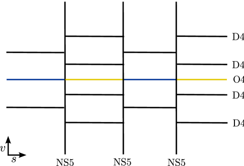
Figure 19: Orientifold D4/NS5-brane embedding of the linear $Sp/SO$ quiver theory of Figure 18.

As illustrated in Figure 19, the orientifold D4/NS5 brane constructions for $Sp$ and $SO$ gauge theories can be naturally extended to any linear quiver theory with alternating $Sp(N-1)$ and $SO(2N)$ gauge groups by introducing an extra NS5-brane for every bifundamental field. For this construction to work it is necessary that the gauge groups alternate as crossing an NS5-brane exchanges one type of orientifold brane with the other. From this string theory embedding we can simply read off the Seiberg-Witten curve.

The Seiberg-Witten curve corresponding to a linear quiver with $Sp(N-1)$ as well as $SO(2N)$ gauge groups can be written in the Gaiotto-form [48]

$$0={\rm det}(v-\boldsymbol{\varphi}_{Sp/SO})=v^{2N}+\varphi_{2}v^{2N-2}+\varphi_{4}v^{2N-4}+\ldots+\varphi_{2N}.$$ (78)

As before, this equation determines the Seiberg-Witten curve as a degree $2N$ covering over the Gaiotto curve. The Hitchin differentials $\varphi_{2k}$ (for $1\leq k\leq N-1$) are of degree $2k$ and encode the vev’s of the Coulomb branch operators ${\rm Tr}(\Phi^{2k})$ of the adjoint scalar $\Phi$ for all gauge groups in the linear quiver. On the other hand, the degree $N$ differential $\varphi_{\tilde{N}}=\sqrt{\varphi_{2N}}$ encodes the vev’s of the operators $\rm{Pfaff}(\Phi)$ for the $SO$ gauge groups in the quiver only. All differentials are also functions of the exactly marginal coupling constants $\tau_{\rm UV}$ and the bare mass parameters, in such a way that the residue of the matrix-valued differential $\boldsymbol{\varphi}_{Sp/SO}$ at each puncture encodes the flavor symmetry of the corresponding matter multiplet.

Figure 20: The Riemann surface on top is the Gaiotto curve corresponding to the linear $Sp(1)/SO(4)$ quiver at the bottom.

It follows from equation (78) that the Gaiotto curve for a linear $Sp(N-1)/SO(2N)$ quiver theory is a genus zero Riemann surface with punctures. For the $Sp(1)/SO(4)$ theory these punctures can be of two types. Either the differential $\varphi_{\tilde{2}}=\sqrt{\varphi_{4}}$ experiences a $\mathbb{Z}_{2}$-monodromy when going around the puncture, or it does not. As before, we call these punctures half-punctures and full punctures, respectively. The puncture representing a bifundamental matter field is a half-puncture. One way to understand this, is to compare the gauge theory quiver to the corresponding Gaiotto curve. As is illustrated in Figure 20 each $Sp(1)$ gauge group corresponds to a tube with a $\mathbb{Z}_{2}$-twist line on the Gaiotto curve, whereas each $SO(4)$ gauge group corresponds to a tube without a $\mathbb{Z}_{2}$-twist line. This implies that at each puncture corresponding to a bifundamental field a $\mathbb{Z}_{2}$-twist line has to end. Notice that the differential $\boldsymbol{\varphi}_{Sp/SO}$ should have a vanishing residue at this half-puncture, since the bifundamental is forced to have zero mass.

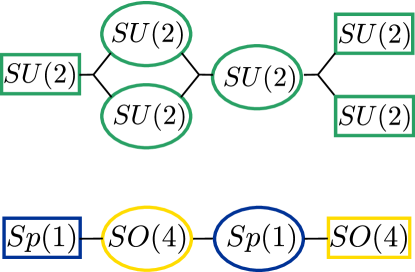
Figure 21: The generalized $SU(2)$ quiver theory, depicted at the top, has isomorphic gauge and flavor symmetries to the linear $SO(4)/Sp(1)$ quiver gauge theory, depicted on the bottom. This picture in particular relates the $SO(4)\times Sp(1)$ bifundamental to the $SU(2)^{3}$ trifundamental.

A remarkable feature of linear $Sp(1)/SO(4)$ quivers is that they are closely related to generalized $SU(2)$ quiver theories [48]. We have already seen that an $Sp(1)$-fundamental can be equivalently represented by an $SU(2)$-fundamental, and an $SO(4)$-fundamental by an $SU(2)^{2}$-bifundamental, as their representations are isomorphic. Even more interestingly, by the same argument an $Sp(1)\times SO(4)$-bifundamental is closely related to a matter multiplet with flavor symmetry group $SU(2)^{3}$. The elementary field with this property is known as the $SU(2)^{3}$-trifundamental, and it consists of eight free half-hypermultiplets in the fundamental representation of the three $SU(2)$ gauge groups [1]. Since the $Sp(1)\times SO(4)$ bifundamental contains eight half-hypermultiplets as well, we expect it to be equivalent to the $SU(2)^{3}$-trifundamental. One example of the relation between linear $Sp(1)/SO(4)$ quivers and generalized $SU(2)$ quiver theories is illustrated in Figure 21.

Similar to our discussion in section 3, we can interpret the $\mathbb{Z}_{2}$-twist lines on the $Sp/SO$ Gaiotto curve as branch cuts. As is illustrated in Figure 22, we find that the Gaiotto curve for the generalized $A_{1}$ quiver theory is a double cover of the Gaiotto curve for the corresponding linear $D_{2}$ quiver theory. This is consistent with the fact that the bifundamental fields cannot carry a mass. Indeed, each half-puncture corresponding to a $Sp(1)\times SO(4)$ bifundamental field lifts to a regular point on the $SU(2)$ Gaiotto curve. Its flavor symmetry had thus better be trivial.

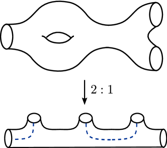
Figure 22: The top picture represents the Gaiotto curve of a generalized $SU(2)$ quiver theory. It is a branched double cover over the Gaiotto curve of the linear $SO(4)/Sp(1)$ quiver theory illustrated in the bottom.

Let us stress that, according to the arguments of section 2, the instanton partition function of a linear quiver theory that contains the $Sp(1)\times SO(4)$ bifundamental will be related to the instanton partition function containing the $SU(2)^{3}$-trifundamental by a non-trivial mapping of marginal gauge couplings. This mapping has a geometric interpretation, according to section 3, as it will relate the complex moduli of the corresponding Gaiotto curves. Studying the instanton partition function of linear $D_{2}$ quiver theories thus sheds light on the understanding of non-linear $A_{1}$ quiver theories. We leave this for future work [56].

5.2 Instanton contribution for the $Sp\times SO$ bifundamental

We continue with finding a contour integrand prescription for the contribution of the $Sp\times SO$ bifundamental matter multiplet. In general, the instanton partition function for a linear quiver gauge theory with gauge group $G=G_{1}\times\cdots\times G_{P}$ can be formulated schematically as

$$Z^{\textrm{inst}}_{k}=\int\prod d\phi_{i}~{}\mathbf{z}_{\textrm{gauge}}^{k}(\phi_{p,i},\vec{a}_{p})~{}\mathbf{z}_{\textrm{bifund}}^{k}(\phi_{p,i},\phi_{q,j},\vec{a}_{p},\vec{a}_{q},\mu)~{}\mathbf{z}_{\textrm{fund}}^{k}(\phi_{p,i},\vec{a}_{p}),$$ (79)

where the three $\mathbf{z}$’s in the integrand refer to the contribution of gauge multiplets, bifundamental and fundamental matter fields, respectively. The only missing ingredient needed to compute the instanton partition function for a linear $D_{2}$-quiver is the contribution of the $Sp\times SO$ bifundamental half-hypermultiplet. This contribution has not yet been studied in the literature.

Remember that a full hypermultiplet consists of two chiral superfields $Q$ and $\tilde{Q}$, where $Q$ and $\tilde{Q}$ are respectively in the representation $R$ and $\bar{R}$ of the gauge group $G$. Since the bifundamental representation $Sp(1)\times SO(4)$ is pseudo-real, the two chiral superfields in a hypermultiplet actually transform under isomorphic representations $R=\bar{R}$.

To find the contour integrand contribution for a half-hypermultiplet, we start out with the same BPS equations as in section 2. Again we consider the vector bundle of solutions ${\cal V}$ to the Dirac equation over the moduli space of instantons ${\cal M}_{G,k}$. This time, however, the solutions need to satisfy an extra reality condition. This implies that the weights of the equivariant torus on the vector bundle ${\cal V}$ should come in pairs $\pm w$. We thus want to argue that we can find the contour integrand for a $Sp(1)\times SO(4)$ bifundamental half-hypermultiplet by taking the appropriate square-root.

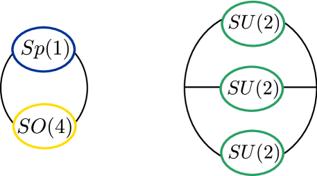
Figure 23: On the left: the quiver diagram for a cyclic $Sp(1)/SO(4)$ quiver gauge theory coupled to two $Sp(1)\times SO(4)$ bifundamentals. The bifundamentals do not have a flavor symmetry group. On the right: the corresponding generalized $SU(2)$ quiver including two $SU(2)^{3}$-trifundamentals.

Let us therefore consider the simplest gauge theory with two $Sp(1)\times SO(4)$ bifundamental half-hypermultiplets. This theory is illustrated on the left in Figure 23. As is illustrated on the bottom of Figure 24, the corresponding Gaiotto curve is a two-punctured torus with a $\mathbb{Z}_{2}$-twist line running between the punctures. The corresponding $A_{1}$ theory is a generalized quiver theory with genus 2.

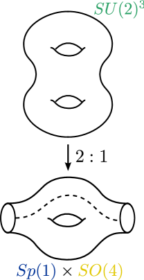
Figure 24: The cover and base Gaiotto-curve corresponding to the $Sp(1)\times SO(4)$ and $SU(2)$ quiver gauge theories illustrated in Figure 23.

Let us define the vector bundles ${\cal V}_{Sp}$ and ${\cal V}_{SO}$ of solutions to the Dirac equation in the fundamental representation of the $Sp$ and $SO$ gauge group, respectively. Since the double copy of a bifundamental half-hypermultiplet is a full bifundamental hypermultiplet, its contribution to the instanton partition function is given by the usual integral

$$\oint_{{\cal M}_{Sp}\times{\cal M}_{SO}}e({\cal V}_{Sp}\otimes{\cal V}_{SO}\otimes{\cal L}\otimes M).$$ (80)

The integrand is the Euler class of the tensor product ${\cal V}_{Sp}\otimes{\cal V}_{SO}\otimes{\cal L}\otimes M$ over the product ${\cal M}_{Sp}\times{\cal M}_{SO}$ of the instanton moduli spaces. In this expression, $M\cong\mathbb{C}$ is the flavor vector space and ${\cal L}$ the half-canonical line bundle over $\mathbb{R}^{4}$.

Following the same strategy as we lined out in section 2 for a usual hypermultiplet, we obtain a contour integrand

$$\mathbf{z}^{Sp,SO}_{k_{1},k_{2},db}(\phi,\psi,\vec{a},\vec{b},m)$$

corresponding to the double copy of the bifundamental half-hypermultiplet. We work this out in appendix A. The parameters $\vec{a}$ and $\vec{b}$ are the Coulomb parameters of the $Sp$ and the $SO$ gauge theory, respectively, whereas $m$ is the mass parameter for the double copy. Since the half-hypermultiplets should be massless we substitute $m=0$. For precisely this value of the mass, the resulting expression indeed turns out to be a complete square

$$\mathbf{z}_{k_{1},k_{2},\textrm{db}}^{Sp,SO}(\phi,\psi,\vec{a},\vec{b},m=0,\epsilon_{1},\epsilon_{2})=\left(\mathbf{z}_{k_{1},k_{2},\textrm{hb}}^{Sp,SO}(\phi,\psi,\vec{a},\vec{b})\right)^{2}.$$ (81)

It is thus natural to identify the square-root $\mathbf{z}_{\textrm{hb}}$ of the double bifundamental with the contribution coming from a $Sp\times SO$-bifundamental half-hypermultiplet. We check this prescription with the CFT shortly.

An interesting observation is that the bifundamental half-hypermultiplet does not introduce additional poles besides those coming from the usual gauge factors $\mathbf{z}_{\rm gauge}$. In analogy to [20], we can therefore view the bifundamental half-hypermultiplet as a mapping

$$\Phi_{a,b_{1},b_{2}}:\widehat{{\cal H}}_{\widetilde{Sp}(1)}\to\widehat{{\cal H}}_{SO(4)}$$ (82)

between two vector spaces $\widehat{{\cal H}}_{\widetilde{Sp}(1)}$ and $\widehat{{\cal H}}_{SO(4)}$, whose bases are parametrized by the poles of the respective gauge multiplet integrands. It is natural to expect that these vector spaces are related to the ${\cal W}$-representation spaces ${\cal H}_{\widetilde{Sp}(1)}$ and ${\cal H}_{SO(4)}$ that we encountered in the previous section. Note that for $Sp$ and $SO$ gauge groups we expect the spaces to be related without any additional $U(1)$ factors. For the original $U(2)$ AGT correspondence this was recently made precise [57]. The structure of the $Sp(1)$ poles is more complicated, however, and it would be interesting to find the exact mapping between the two spaces.

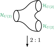
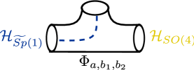
Figure 25: The instanton contribution for the $U(2)^{3}$ trifundamental can be represented as a linear map $Z^{\rm inst}:\mathcal{H}_{U(2)}\to\mathcal{H}_{U(2)}\times\mathcal{H}_{U(2)}$. Similarly, and correspondingly, the $Sp(1)\times SO(4)$ bifundamental field defines a linear map $Z^{\rm inst}:\widehat{\mathcal{H}}_{\widetilde{Sp}(1)}\to\widehat{\mathcal{H}}_{SO(4)}$.

5.3 Test of the $Sp(1)\times SO(4)$ AGT correspondence

Since we know the Gaiotto curve corresponding to alternating $SO/Sp$ quiver theories, we can extend the correspondence between $SO/Sp$ gauge groups and ${\cal W}$ blocks. We are now ready to check this correspondence. At the same time this will also serve as an additional check that our expression for the half-hypermultiplet is correct. Consider thus the $SO/Sp$ theory illustrated in Figure 18, with a single bifundamental half-hypermultiplet, two fundamental $Sp(1)$-hypermultiplets and one fundamental $SO(4)$-hypermultiplet.

5.3.1 $Sp(1)\times SO(4)$ instantons

Let us first compute the instanton partition function of this linear quiver theory. The first non-trivial term comes from $(k_{1},k_{2})=(1,1)$. In the unrefined case $\epsilon_{1}=-\epsilon_{2}=\hbar$, it is given by

$$Z^{\rm inst}_{1,1}=-\frac{m_{1}m_{2}b_{1}b_{2}\left(\left(m_{3}^{2}-b_{1}^{2}\right)\left(-a^{2}+b_{1}^{2}\right)\left(-\hbar^{2}+b_{1}^{2}\right)+\left(a^{2}-b_{2}^{2}\right)\left(-m_{3}^{2}+b_{2}^{2}\right)\left(-\hbar^{2}+b_{2}^{2}\right)\right)}{8a^{2}\hbar^{4}\left(b_{1}^{2}-b_{2}^{2}\right)^{2}}~{}$$

where $m_{1},m_{2}$ are the masses of the $Sp(1)$-fundamentals, $m_{3}$ is the mass of the $SO(4)$-fundamental and $a,b_{i}$ are the Coulomb branch parameters of $Sp(1)$ and $SO(4)$ respectively.

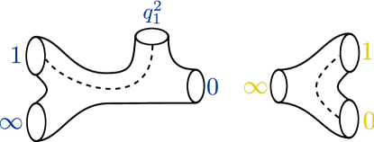
Figure 26: Decomposition of the $Sp(1)\times SO(4)$ Gaiotto curve that we used for computing the corresponding ${\cal W}(2,2)$-block.

5.3.2 $Sp(1)\times SO(4)$ correlators

The correlator that corresponds to the (mirror of the) quiver illustrated in Figure 18 is the following:

$$\langle V_{1}(\infty)\sigma(1)\sigma(q_{1}^{2})\sigma(q_{1}^{2}q_{2})\hat{V}_{2}(0)\rangle$$ (83)

For notational simplicity we have introduced the variables $q_{1}=q_{Sp(1)}/4$ and $q_{2}=q_{SO(4)}$. A single term in the chiral block is then expanded as (see Figure 26)

$$\langle V_{1}(\infty)\sigma(1)\sigma(q_{1})V^{A,B}(0)\rangle\langle V^{A,B}(\infty)\sigma(q_{1}^{2}q_{2})\hat{V}_{2}(0)\rangle\\ =\langle V_{1}(\infty)\sigma(1)\sigma(q_{1}^{2})V^{A,B}(0)\rangle(q_{1}^{2}q_{2})^{h_{A}+n_{A}+h_{B}+n_{B}}\langle V^{A,B}(\infty)\sigma(1)\hat{V}_{2}(0)\rangle$$ (84)

To compute the rightmost correlator, we can proceed as in subsection 4.4.2 and map it to a cover correlator of the form (74). Due to the corrections we will get something of the form

$$\langle V^{A,B}(\infty)\sigma(1)\hat{V}_{2}(0)\rangle=\left(\frac{1}{2}\right)^{n_{A}+n_{B}}\mathbf{\tilde{C}}^{h_{A},h_{B};h_{1}}_{I_{A},I_{B},\bullet}+\textrm{lower descendant corrections}\ .$$ (85)

The correlator is thus the same as the one we computed in the section on $SO(4)$.

The four point correlator on the left we treat as in the $Sp(1)$ case, i.e. we apply the cover map (67). The only difference is then that $V^{A,B}$ is a descendant field, and thus like in the $SO(4)$ computation picks up corrections from the map:

$$V^{A,B}(0)=V\left(\left(\frac{-1+q_{1}^{2}}{2q_{1}}\right)^{L_{0}}\exp\left[\left(\frac{3}{4}+\frac{1}{4q_{1}^{2}}\right)L_{1}\right]\exp\left[\frac{(-1+q_{1}^{2})^{2}}{16q_{1}^{4}}L_{2}\right]\cdots\phi^{A},q_{1}\right)\\ \times V\left(\left(-\frac{-1+q_{1}^{2}}{2q_{1}}\right)^{L_{0}}\exp\left[\left(\frac{3}{4}+\frac{1}{4q_{1}^{2}}\right)L_{1}\right]\exp\left[\frac{(-1+q_{1}^{2})^{2}}{16q_{1}^{4}}L_{2}\right]\cdots\phi^{B},-q_{1}\right)$$ (86)

This expression is however different in two ways from the corresponding $SO(4)$ expression (4.4.2). First, the vertex operators are at the positions $\pm q_{1}$. We decompose the four punctured correlator on the cover in usual way, and move them to the standard positions $\pm 1$ using the map $z\mapsto zq_{1}^{-1}$. This simply leads to an additional prefactor $q_{1}^{-L_{0}}$ in equation (86). To pull out the standard prefactor $q_{1}^{h_{A,B}}$, it is useful to commute this prefactor all the way to the left, which we can do by using the identity

$$x^{L_{0}}L_{n}=\frac{L_{n}}{x^{n}}x^{L_{0}}\ .$$ (87)

This leads to the expression

$$\left(\frac{-1+q_{1}^{2}}{2q_{1}^{2}}\right)^{h_{A}+n_{A}+h_{B}+n_{B}}\times$$ (88)

$$\langle\phi|V\left(\exp\left[\frac{1+3q_{1}^{2}}{2(-1+q_{1}^{2})}L_{1}\right]e^{L_{2}/4}\cdots\phi^{A},1\right)V\left(\exp\left[-\frac{1+3q_{1}^{2}}{2(-1+q_{1}^{2})}L_{1}\right]e^{L_{2}/4}\cdots\phi^{B},-1\right)\rangle\ .$$

Note that the $q_{1}^{2(h_{A}+n_{A}+h_{B}+n_{B})}$ in the denominator of the prefactor exactly cancels the corresponding factor of $q_{1}$ in equation (84). The numerator of the prefactor on the other hand is the same prefactor that we already found in the $Sp(1)$ computation.

Let us now actually compute the first few terms of the chiral block. The terms where of order zero in either $q_{Sp(1)}$ or $q_{SO(4)}$ are are simply the same as in the $SO(4)$ and $Sp(1)$ computation. We therefore consider the simplest new term, $q_{Sp(1)}q_{SO(4)}$. This means in particular that we can neglect all terms of order $q_{1}^{2}$ in the expression (88), so that the vertex operators no longer depend on $q_{1}$. Since we would like to rewrite this expression in terms of the three point coefficients $\tilde{\mathbf{C}}$ defined above, we need move the field $\phi$ from $\infty$ to 0 by applying the map $z\mapsto z^{-1}$. Note that we pick up some additional corrections due to the fact that the fields at $\pm 1$ are descendant fields. In total (88) thus becomes

$$(2^{-n_{A}-n_{B}})\langle V\left(e^{3L_{1}/2}e^{L_{2}/4}\cdots\phi^{A},1\right)V\left(e^{-3L_{1}/2}e^{L_{2}/4}\cdots\phi^{B},-1\right)|\phi\rangle\ .$$ (89)

Not surprisingly, this is the same expression that we had found in the $SO(4)$ case. From this, the term of order $q_{Sp(1)}q_{SO(4)}$ is

$$\frac{\mathbf{\tilde{C}}^{h_{1},h_{2};h_{a}}_{\bullet,\bullet,\square}}{2h_{a}}\frac{1}{4}\Bigl{(} \frac{(\mathbf{\tilde{C}}^{h_{A},h_{B};h_{a}}_{\square,\bullet,\square}+3h_{A}\mathbf{\tilde{C}}^{h_{A},h_{B};h_{a}}_{\bullet,\bullet,\square})(\mathbf{\tilde{C}}^{h_{A},h_{B};h_{3}}_{\square,\bullet,\bullet}+3h_{A})}{2h_{A}}$$ (90)

$$\qquad\qquad+\frac{(\mathbf{\tilde{C}}^{h_{A},h_{B};h_{a}}_{\bullet,\square,\square}-3h_{B}\mathbf{\tilde{C}}^{h_{A},h_{B};h_{a}}_{\bullet,\bullet,\square})(\mathbf{\tilde{C}}^{h_{A},h_{B};h_{3}}_{\bullet,\square,\bullet}-3h_{B})}{2h_{B}}\Bigr{)}.$$

Similar computations lead to higher order terms. We have checked that the instanton partition function and the chiral block agrees up to order $(k_{1},k_{2})=(1,2)$ up to a moduli independent spurious factor, using the same identifications of the previous examples.

Appendix

Appendix A Instanton counting

In this appendix we summarize and extend methods to derive the instanton counting formulae for general gauge groups and matter in several representations. In particular, we find the contour integral prescription for half-bifundamental $Sp-SO$ hypermultiplets.

A.1 ADHM construction

Let $E$ be a rank $N$ complex vector bundle on $\mathbb{R}^{4}$ with a connection $A$ and a framing at infinity. The framing is an isomorphism of the fiber at infinity with $\mathbb{C}^{N}$. The ADHM construction studies the moduli space ${\cal M}_{k}$ of connections $A$ on the bundle $E$ that satisfy the self-dual instanton equation $F^{+}(A)=0$, up to gauge transformations that are trivial at infinity. It turns out that this moduli space can be realized as a hyperkähler quotient of linear data.

$U(N)$ gauge group

Figure 27: Quiver representation of the $U(N)$ ADHM quiver. The vector spaces $V$ and $W$ are $k$ and $N$-dimensional, respectively, with a natural action of the dual group $U(k)$ and the framing group $U(N)$. The maps $B_{1}$, $B_{2}$, $I$ and $J$ are linear.

For the gauge group $G=U(N)$ the linear data consists of four linear maps

$$(B_{1},B_{2},I,J)\in\mathbf{X}=\mathrm{Hom}(V,V)\oplus\mathrm{Hom}(V,V)\oplus\mathrm{Hom}(W,V)\oplus\mathrm{Hom}(V,W),$$ (91)

where $V$ and $W$ are two complex vector spaces of dimension $k$ and $N$, respectively. This linear data is summarized in an ADHM quiver diagram in Figure 27. The vector space $W$ is isomorphic to the fiber of $E$ (which in our case is of rank $N$). It is best thought of as the fiber at infinity, as there is a natural action of the framing group $U(N)$ on it, which physically can be thought of as the large gauge transformations at infinity. The tensor product of the vector space $V$ with the half canonical bundle $K_{\mathbb{C}^{2}}^{1/2}$ on $\mathbb{C}^{2}\cong\mathbb{R}^{4}$, on the other hand, can be identified with the space of normalizable solutions to the Dirac equation in the background of the instanton gauge field $A$. Since the instanton number $k=1/8\pi^{2}\int F_{A}\wedge F_{A}$ is given by the second Chern class of $E$, it follows from index theorems that this space has dimension $k$, as we advertised above. In particular it carries in a natural way the action of the dual group $U(k)$. More algebraically, the vector space $V$ itself is isomorphic to the cohomology group $H^{1}(E)$.

The framing group $U(N)$ and the dual group $U(k)$ thus act naturally on the linear ADHM data. Setting the three real moment maps

$$\mu_{\mathbb{R}} = [B_{1},B_{1}^{\dagger}]+[B_{2},B_{2}^{\dagger}]+II^{\dagger}-J^{\dagger}J$$ (92)

$$\mu_{\mathbb{C}} = [B_{1},B_{2}]+IJ,$$ (93)

to zero gives the so-called ADHM equations. The ADHM construction identifies the instanton moduli space ${\cal M}_{k}^{U(N)}$ with the hyperkähler quotient of the solutions $\mathbf{X}$ to those equations by the dual group,

$${\cal M}^{U(k)}_{k}=\mathbf{X}//U(k)\equiv\mu^{-1}(0)/U(k).$$ (94)

From a physical perspective the ADHM construction can be most natural understood using D-branes. We can engineer the moduli space of $k$ instantons in the four-dimensional $U(N)$ theory by putting $k$ D$(p-4)$-branes on top of $N$ D$p$-branes. The D$(p-4)$-branes appear as zero-dimensional instantons on the transverse four-dimensional manifold. The maps $(B_{1},B_{2},I,J)$ can be understood as the zero-modes of D$(p-4)-$D$(p-4)$), D$p-$D$(p-4)$ and D$(p-4)-$D$p$ open strings, respectively, and the ADHM equations are the D-term conditions. The ADHM quotient can thus be identified with the moduli space of the Higgs branch of the $U(k)$ gauge theory on the D$(p-4)$-branes.

Since the above quotient is highly singular due to small instantons, we change it by giving non-zero value to the Fayet-Illiopolous term $\zeta$. This is equivalent to turning on NS 2-form field on the D$p$-branes, and the resulting desingularized quotient can be interpreted as a moduli space of non-commutative instantons [69].

To perform our computations another, equivalent way of representing the ADHM construction will be useful. Let us introduce the spinor bundles ${\cal S}^{\pm}$ of positive and negative chirality on $\mathbb{R}^{4}$, and for brevity denote the half canonical bundle by ${\cal L}=K_{\mathbb{C}^{2}}^{1/2}$. Consider the sequence

$$V\otimes L^{-1}\rightarrow^{\sigma}\hskip 5.69054pt\begin{array}[]{c}V\otimes S^{-}\\ \oplus\\ W\end{array}\rightarrow^{\tau}\hskip 5.69054ptV\otimes L\,,$$ (98)

where $S^{-}$ and $L$ are the fibers of the bundles ${\cal S}^{-}$ and ${\cal L}$, respectively. Although these can all be trivialized, they are non-trivial equivariantly. We thus need to keep track of them for later. The mappings $\sigma$ and $\tau$ are defined by

$$\sigma=\left(\begin{array}[]{c}z_{1}-B_{1}\\ z_{2}-B_{2}\\ J\end{array}\right),\qquad\tau=\left(\begin{array}[]{ccc}-z_{2}+B_{2},&z_{1}-B_{1},&I\end{array}\right),$$ (103)

where $(z_{1},z_{2})$ are coordinates on $\mathbb{C}^{2}$. From the ADHM equations it follows that $\tau\circ\sigma=0$, so that the sequence (98) is a chain complex. Since $\sigma$ is injective and $\tau$ surjective, it is a so-called monad.

Notice that the vector space $V\otimes L^{-1}$ at the first position of the sequence (98) fixes the vector spaces at the remainder of the sequence. The fields $B_{1}$ and $B_{2}$ are coordinates on $\mathbb{C}^{2}$ and thus map $V\otimes L^{-1}\to V\otimes S^{-}$. The fields $I$ and $J$ are the two scalar components of an ${\cal N}=2$ hypermultiplet, that properly speaking transform as sections of the line bundle ${\cal L}$.

To recover the vector bundle $E$, we vary the cohomology space $(\rm{Ker}\,\tau)/(\rm{Im}\,\sigma)$ over $\mathbb{C}^{2}$, which gives indeed a vector bundle whose fiber at infinity is equal to $W$. One can also show that the curvature of this bundle is self-dual and that it has instanton number $k$. Even better, every solution of the self-dual instanton equations can be found in this way.

We are now ready to construct the main tool in our computation. This is the universal bundle ${\cal E}$ over the instanton moduli space ${\cal M}^{U(N)}_{k}\times\mathbb{R}^{4}$. The universal bundle is obtained by varying the ADHM-parameters of the maps in the complex (98). It has the property that

$${\cal E}_{A,z}=E_{z},$$ (104)

i.e. its fiber over an element $A\in{\cal M}^{U(N)}_{k}$ is the total space of the bundle $E$ with connection $A$. Remember that the bundle $E$ has fiber $W$ at infinity in $\mathbb{R}^{4}$ and that the vector space $V$ of solutions to the Dirac equations is related to its first cohomology $H^{1}(E)$. The vector spaces $V$ and $W$ can be extended to bundles ${\cal V}$ and ${\cal W}$ over the instanton moduli space. We can then easily compute the Chern character of the universal bundle ${\cal E}$ from its defining complex (98) as

$$\rm{Ch}({\cal E})=\rm{Ch}({\cal W})+\rm{Ch}({\cal V})\left(\rm{Ch}({\cal S}^{-})-\rm{Ch}({\cal L})-\rm{Ch}({\cal L}^{-1})\right).$$ (105)

$SO/Sp$ gauge groups

The construction for $SO(N)$ and $Sp(N)$ gauge groups is very similar. We define $Sp(N)$ to be the special unitary transformations on $\mathbb{C}^{2N}$ that preserve its symplectic structure $\Phi_{s}$, and $SO(N)$ the special unitary transformations on $\mathbb{C}^{N}$ that preserve its real structure $\Phi_{r}$.

Figure 28: Quiver representation of the $Sp(N)$ ADHM quiver. The vector spaces $V$ and $W$ are $k$ and $2N$-dimensional, respectively. $V$ has a real structure $\Phi_{r}$ and a natural action of the dual group $SO(k)$, whereas $W$ has a symplectic structure $\Phi_{s}$ and a natural action of the framing group $Sp(N)$. The maps $B_{1}$, $B_{2}$ and $J$ are linear.

For $Sp(N)$ the linear data that is needed to define the ADHM complex consists of

$$(B_{1},B_{2},J)\in\mathbb{Y}=\mathrm{Hom}(V,V)\oplus\mathrm{Hom}(V,V)\oplus\mathrm{Hom}(V,W),$$ (106)

where $V$ and $W$ are a complex $k$ and $2N$-dimensional vector space, resp., together with a real structure $\Phi_{r}$ on $V$ and a symplectic structure $\Phi_{s}$ on $W$. This is illustrated as a quiver diagram in Figure 28. The dual group is given by $O(k)$, so that the moduli space of $Sp(N)$ instantons is given by

$${\cal M}^{Sp(N)}_{k}=\{(B_{1},B_{2},J)\,|\,\Phi_{r}B_{1},\Phi_{r}B_{2}\in S^{2}V^{*},\,\Phi_{r}[B_{1},B_{2}]-J^{*}\Phi_{s}J=0\}/O(k).$$ (107)

Figure 29: Quiver representation of the $SO(N)$ ADHM quiver. The vector spaces $V$ and $W$ are $2k$ and $N$-dimensional, respectively. $V$ has a symplectic structure $\Phi_{s}$ and a natural action of the dual group $Sp(k)$, whereas $W$ has a real structure $\Phi_{r}$ and a natural action of the framing group $SO(N)$. The maps $B_{1}$, $B_{2}$ and $J$ are linear.

For $SO(N)$ we just need to replace $V$ and $W$ by a complex $2k$ and $N$-dimensional vector space, resp., as well as change the role of symplectic structure and the real structure. This is illustrated as a quiver diagram in Figure 29. The dual group is given by $Sp(k)$, so that the moduli space of $SO(N)$ instantons is given by

$${\cal M}^{SO(N)}_{k}=\{(B_{1},B_{2},J)\,|\,\Phi_{s}B_{1},\Phi_{s}B\in\wedge^{2}V^{*},\,\Phi_{s}[B_{1},B_{2}]-J^{*}\Phi_{r}J=0\}/Sp(k).$$ (108)

A subtle issue for the above moduli spaces is that there is no appropriate Gieseker desingularization which resolves the singularity due to the zero-sized instantons (as in the case of $U(N)$). One way to understand this is by considering the string theory embedding. The above ADHM constructions can be obtained by considering D$p$-D$(p-4)$ system and also adding an $O^{\pm}p$ plane on the top of the D$p$ branes. In the case of $U(N)$, the non-commutativity parameter that we introduce is coming from the NS 2-form field on the $Dp$-brane. But, the orientifold makes it impossible to turn on the background NS 2-form field. So we cannot resolve the singularity in the same way. An alternative way to resolve the singularity was studied by [70], but a physical understanding of this procedure is still lacking. Nevertheless, we will see that the equivariant volume of the moduli space can be obtained without explicitly resolving the singularity [26]. This formula is verified mathematically using Kirwan’s formula of the equivariant volume of the symplectic quotient [66].

We can then again represent any $Sp(N)$ instanton solution $E$ as the cohomology bundle of the sequence

$$V\otimes L^{-1}\longrightarrow^{\sigma}\hskip 8.53581pt\begin{array}[]{c}V\otimes S^{-}\\ \oplus\\ W\end{array}\longrightarrow^{\sigma^{*}\beta^{*}}\hskip 11.38109ptV^{*}\otimes L,$$ (112)

where the mappings $\sigma$ and $\beta$ are defined by

$$\sigma=\left(\begin{array}[]{c}z_{1}-B_{1}\\ z_{2}-B_{2}\\ J\end{array}\right),\qquad\beta=\left(\begin{array}[]{ccc}0&\Phi_{r}&0\\ -\Phi_{r}&0&0\\ 0&0&\Phi_{s}\end{array}\right).$$ (119)

The ADHM equations ensure that $\sigma^{*}\beta^{*}\sigma=0$, and the sequence (112) is another monad. Analogously to the $U(N)$ example, when varying the ADHM-parameters in the complex (112) we find the universal bundle ${\cal E}_{Sp(N)}$. $V$ is the $k$-dimensional solution space of the $Sp(N)$ Dirac operator on $\mathbb{C}^{2}$, which carries a real structure, and $W$ is the fiber of $E$ at infinity, and hence carries a symplectic structure.

Similarly, any $SO(N)$ instanton solution $E$ can be represented as the cohomology bundle of the complex (112) as well, once we exchange $\Phi_{r}$ with $\Phi_{s}$ in the definition of the map $\beta$. The resulting complex is a short exact sequence, since according to the ADHM equations $\sigma^{*}\beta^{*}\sigma=0$. By varying the ADHM-parameters we find the $SO(N)$ universal bundle ${\cal E}_{SO(N)}$. Note that $V$ is the $2k$-dimensional solution space of the $SO(N)$ Dirac operator on $\mathbb{C}^{2}$, which carries a symplectic structure, whereas $W$ is the fiber of $E$ at infinity, and hence carries a real structure.

A.2 $\Omega$-background and equivariant integration

Let us start with a supersymmetric ${\cal N}=2$ gauge theory without matter. This theory can be topologically twisted (using the so-called Donaldson twist), so that its BPS equation is the instanton equation $F_{A}^{+}=0$. The instanton partition function is given by an integral over the moduli space ${\cal M}^{\rm inst}_{k}$,

$$Z^{\rm inst}=\sum_{k}q^{k}\oint_{{\cal M}^{\rm inst}_{k}}1\ ,$$ (120)

where $\oint 1$ indicates the formal volume of the hyperkähler quotient.

If we add matter multiplets to the gauge theory, say a single ${\cal N}=2$ hypermultiplet, the BPS equations turn into the monopole equations

$$F_{A,\mu\nu}^{+}+\frac{i}{2}\ \overline{q}_{\alpha}\Gamma^{\hskip 9.95845pt\alpha}_{\mu\nu\hskip 5.69054pt\beta}q^{\beta} =0,$$ (121)

$$\sum_{\mu}\Gamma^{\mu}_{\dot{\alpha}\alpha}D_{A,\mu}q^{\alpha} =0.$$

Here, $\Gamma^{\mu}$ are the Clifford matrices and $\sum_{\mu}\Gamma^{\mu}D_{A,\mu}$ is the Dirac operator in the instanton background for the connection $A$. Furthermore, $q^{\alpha}$ is the lowest component of the twisted hypermultiplet. The representation of the connection $A$ in the connection $D_{A}$ is determined by the representation of the gauge group that the hypermultiplet is in. As is argued in section 3.4 of [35], it is possible to deform the action in a Q-exact way such that the first equation gets an extra factor

$$F_{A,\mu\nu}^{+}+\frac{i}{2t}\ \overline{q}_{\alpha}\Gamma^{\hskip 9.95845pt\alpha}_{\mu\nu\hskip 5.69054pt\beta}q^{\beta} =0,,$$

for an arbitrary value of $t$. Taking the limit $t\to\infty$ reduces this BPS equation to the selfdual instanton equation. Given an instanton solution $A$, the remainder of the action is forced to localize onto solutions of the Dirac equation in the background of $A$. The kernel of the Dirac operator thus forms a fiber over the instanton moduli space ${\cal M}^{\rm inst}$.

Let us start out by adding a single hypermultiplet in the fundamental representation of the gauge group. Remember that the corresponding kernel was already encoded in the vector bundle ${\cal V}\otimes{\cal L}$ in the original ADHM construction. $N_{f}$ hypers are simply described by the tensor product of $N_{f}$ vector bundles ${\cal V}$. Each individual factor then carries the usual action of the dual group. Moreover, there is now also a natural action of the flavor symmetry group. By general arguments (see for example [71]) this partition function then localizes to the integral

$$Z^{\rm inst}=\sum_{k}q^{k}\oint_{{\cal M}^{\rm inst}_{k}}e({\cal V}\otimes{\cal L}\otimes M)$$ (122)

of the Euler class of the vector bundle ${\cal V}\otimes{\cal L}$ of solutions to the Dirac equation over the moduli space ${\cal M}^{\rm inst}$. The vector space $M=\mathbb{C}^{N_{f}}$ encodes the number of flavors.

Let us now discuss how to compute this partition function. First, however, note that (122) diverges. We will implicitly take care of the UV divergence in the next steps by computing a holomorphic character [26], but we also need to deal with IR divergences: the instanton moduli space has flat directions where the instantons move off to infinity. One way to regularize the instanton partition function is to introduce the so-called $\Omega$-background, where we use equivariant integration with respect to the torus

$$\mathbf{T}^{2}_{\epsilon_{1},\epsilon_{2}}=U(1)_{\epsilon_{1}}\times U(1)_{\epsilon_{2}},$$ (123)

that acts on $\mathbb{R}^{4}=\mathbb{C}\oplus\mathbb{C}$ by a rotation $(z_{1},z_{2})\to(e^{i\epsilon_{1}}z_{1},e^{i\epsilon_{2}}z_{2})$ around the origin. This forces the instantons to be localized at the origin of $\mathbb{R}^{4}$. The resulting $\Omega$-background is denoted by $\mathbb{R}^{4}_{\epsilon_{1},\epsilon_{2}}$. The partition function in the $\Omega$-background is defined by equivariantly integrating with respect to the $\mathbf{T}^{2}_{\epsilon_{1},\epsilon_{2}}$–action.

We have already introduced the other components of the equivariance group: The torus $\mathbf{T}^{N}_{a}$ of the gauge group $G$ acting on the fiber $W$ with weights $a_{l}$, the torus $\mathbf{T}^{k}_{\phi_{i}}$ of the dual group acting on $V$ with weights $\phi_{i}$, and lastly the torus $\mathbf{T}^{N_{f}}_{m}$ of the flavor symmetry group acting on the flavor vector space $M$ with weights $m_{j}$. In total, we perform the equivariant integration with respect to the torus

$$\mathbf{T}=\mathbf{T}^{2}_{\epsilon_{1},\epsilon_{2}}\times\mathbf{T}^{N}_{a}\times\mathbf{T}^{k}_{\phi}\times\mathbf{T}^{N_{f}}_{m}\ .$$ (124)

The instanton partition function in the $\Omega$-background is thus defined as the equivariant integral

$$Z(a,m,\epsilon_{1},\epsilon_{2})=\sum_{k}q^{k}\oint_{{\cal M}_{k}}e_{\mathbf{T}}({\cal V}\otimes{\cal L}\otimes M)\,,$$ (125)

where $e_{\mathbf{T}}$ is the equivariant Euler class with respect to the torus $\mathbf{T}$. We will evaluate (125) in two steps, using the fact that ${\cal M}_{k}$ is given by the solutions $\mu^{-1}(0)$ to the ADHM equations quotiented by the dual group $G^{D}_{k}$. We will thus first perform the equivariant integral over $\mu^{-1}(0)$, and then take care of the quotient by integrating out $G^{D}_{k}$, which gives a multiple integral over $\phi_{i}$.

To perform the first part of the above integral, we apply the famous equivariant localization theorem, which tells us that the integral only depends on the fixed points of the equivariant group and its weights at those points. This then leads to a rational function in all the weights.

More precisely, suppose that the action of the element $t\in\mathfrak{t}$ on the integration space ${\cal M}$ (which is represented by a vector field $V_{t}$) has a discrete number of fixed points $f$. Then the equivariant localization theorem says that

$$\int_{{\cal M}}\alpha=\sum_{f}\frac{\iota^{*}\alpha}{\prod_{k}w_{k}[t](f)},$$ (126)

where $\iota$ embeds the fixed point locus in ${\cal M}$ and where $w_{k}[t](f)$ are the weights of the action of the vector field $V_{t}$ on the tangent space to the fixed point $f\in{\cal M}$. If we apply the localization theorem to the integral (125), the denominator of the resulting expression contains a product of weights of the torus action on the tangent bundle to the instanton moduli space. Its numerator is given by another product of weight of the torus action on the bundle ${\cal V}\otimes{\cal L}\otimes M$ of Dirac zero modes.

Let us start with computing the weights in the numerator, and for convenience restrict the matter content to a single hypermultiplet in the fundamental representation of the gauge group. Since the bundle in the numerator is the kernel of the Dirac operator, we can equally well obtain these weights from the equivariant index $\textrm{Ind}_{\mathbf{T}}=\sum_{k}n_{k}e^{iw_{k}}$ of the Dirac operator. For the purpose of (126), the sum over weights can be translated into a product by the formula

$$\sum_{k}n_{k}e^{iw_{k}}\to\prod_{i}(w_{k})^{n_{k}}.$$ (127)

To compute the equivariant index $\textrm{Ind}_{\mathbf{T}}$ of the Dirac operator coupled to the instanton background, we make use of the equivariant version of Atiyah-Singer index theorem. It is given by

$$\textrm{Ind}_{\mathbf{T}}=\int_{\mathbb{C}^{2}}\textrm{Ch}_{\mathbf{T}}({\cal E}\otimes{\cal L})\,\textrm{Td}_{\mathbf{T}}(\mathbb{C}^{2})=\frac{\textrm{Ch}_{\mathbf{T}}({\cal E}\otimes{\cal L})|_{z_{1}=z_{2}=0}}{(e^{i\epsilon_{1}}-1)(e^{i\epsilon_{2}}-1)},$$ (128)

where ${\cal E}$ is the universal bundle over the instanton moduli space ${\cal M}_{k}$ that we constructed in the previous section. Remember that the fiber of ${\cal E}$ over an element $A$ in the instanton moduli space is given by the total space of the instanton bundle $E$ with connection $A$. The second equality is obtained by applying the equivariant localization theorem and using the equivariant Todd class of $\mathbb{C}^{2}$ equals

$$\textrm{Td}_{\mathbf{T}}(\mathbb{C}^{2})=\frac{\epsilon_{1}\epsilon_{2}}{(e^{i\epsilon_{1}}-1)(e^{i\epsilon_{2}}-1)},$$ (129)

where the weights of the action of $\mathbf{T}_{\epsilon_{1},\epsilon_{2}}$ on $\mathbb{C}^{2}$ are $\epsilon_{1}$ and $\epsilon_{2}$.

The purpose of all of this was to reduce everything to the equivariant Chern character of the universal bundle ${\cal E}$, for which have found the simple expression (105) in terms of the Chern characters of the vector bundles ${\cal W}$, ${\cal V}$, ${\cal L}$ and ${\cal S}$. We can easily obtain the weights of the torus $\mathbf{T}$ on these bundles, so that we can compute the contribution of a fundamental hypermultiplet. We will write down explicit expressions in a moment, but let us first explain how to obtain the weights for other representations.

If we instead wish to extract the weights for an anti-fundamental hyper we just need replace the equivariant character for universal bundle ${\cal E}$ by its complex conjugate ${\cal E}^{*}$. Other representations that are tensor products of fundamentals and anti-fundamentals (or symmetric or antisymmetric combinations thereof) can be obtained similarly. For instance, the adjoint representation for a classical gauge group can be expressed as some product of the fundamental and the anti-fundamental representation. This product is the tensor product for $U(N)$, the anti-symmetric product for $SO(N)$ and the symmetric product for $Sp(N)$. Note that in those cases we also obtain the representations of the dual groups. We thus obtain the weights for an adjoint hypermultiplet by computing the character of the appropriate product of the universal bundle and its complex conjugate. The weights for the gauge multiplet are the same as for an adjoint hypermultiplet, but end up in the denominator of the contour integral instead of the numerator. This is consistent with the localization formula (125), as the tangent space to the instanton moduli space can be expressed as the same product of the universal bundle and its dual.

Once we obtain the index, we can extract the equivariant weights from it by using the rule (127). Finally, we need to integrate out the dual group $G^{D}_{k}$. This leads to a multiple integral over $d\phi_{i}$ along the real axis. We will absorb factors appearing from this integration such as the Vandermonde determinant of the Haar measure and the volume of the dual group into the contribution of the gauge multiplet $\mathbf{z}^{k}_{\rm gauge}$. The resulting integrand actually has poles on the real axis, which we cure by giving small imaginary parts to the equivariance parameters. We will describe this in more detail once we turn to the actual evaluation of such integrals. Since the integrand obtained is a rational function in the parameters of $G^{D}_{k}$, we can convert the integral into a contour integral around the poles of the integrand. In total the equivariant integral (125) over the moduli space thus reduces to

$$Z_{k}(a,m,\epsilon_{1},\epsilon_{2})=\oint\prod_{i}d\phi_{i}\prod_{R}\mathbf{z}^{k}_{R}(\phi_{i},a,m,\epsilon_{1},\epsilon_{2}),$$ (130)

where $\mathbf{z}^{k}_{R}$ are the integrands that represent the matter content of the gauge theory and where the $\phi_{i}$’s parametrize the dual group. We will discuss which poles (130) is integrated around shortly.

Equivariant index for $U(N)$ theories

Let us see how this works out explicitly for gauge group $U(N)$. We first have a look at the weights of the torus $\mathbf{T}^{2}_{\epsilon_{1},\epsilon_{2}}$ at the fibers of the half-canonical bundle ${\cal L}$ and the spinor bundles ${\cal S}^{\pm}$ at the origin of $\mathbb{R}^{4}$. Remember that the torus $\mathbf{T}^{2}_{\epsilon_{1},\epsilon_{2}}$ acts on the coordinates $z_{1}$ and $z_{2}$ with weights $\epsilon_{1}$ and $\epsilon_{2}$ respectively. It thus acts on local sections $s$ of the half-canonical bundle as

$$s\in{\cal L}: \quad s\mapsto e^{i\epsilon_{+}}s\,,$$

with $\epsilon_{\pm}=\frac{e_{1}\pm e_{2}}{2}$. Local sections of the four-dimensional spinor bundles ${\cal S}^{\pm}$ can be written in terms of those of the two-dimensional spinor bundles on $\mathbb{R}^{2}$. Since the weights of the torus $\mathbf{T}^{1}_{\epsilon_{j}}$ on the local sections of the two spinor bundles on $\mathbb{R}^{2}$ are $\pm\frac{\epsilon_{j}}{2}$, the torus $\mathbf{T}^{2}_{\epsilon_{1},\epsilon_{2}}$ acts on local sections $\psi_{\pm}$ of the four-dimensional spinor bundle as

$$\psi_{\pm}\in{\cal S}^{\pm}: \quad\psi_{\pm}\mapsto\textrm{diag}(e^{i\epsilon_{\pm}},e^{-i\epsilon_{\pm}})\,\psi_{\pm}\,.$$

Let us continue with the weights of the equivariant torus $\mathbf{T}^{N}_{a}\times\mathbf{T}^{k}_{\phi}$. The equivariant torus then acts on the linear ADHM data as

$$v\in V: \quad v\mapsto\textrm{diag}\,(e^{i\phi_{1}},\cdots,e^{i\phi_{k}})\,v\,,$$

$$w\in W: \quad w\mapsto\textrm{diag}\,(e^{ia_{1}},\cdots,e^{ia_{N}})\,w\,.$$

Combining all weights and using the formula (105), we find that the equivariant Chern character of the universal bundle ${\cal E}_{U(N)}$ is given by

$$\textrm{Ch}_{\mathbf{T}}({\cal E}_{U(N)})|_{z_{1}=z_{2}=0} = \sum_{l=1}^{n}e^{ia_{l}}-(e^{i\epsilon_{1}}-1)(e^{i\epsilon_{2}}-1)\sum_{i=1}^{k}e^{i\phi_{i}-i\epsilon_{+}}.$$ (131)

Using the index formula (128) we have now computed the contribution for a fundamental massless hypermultiplet. As we explained before we can easily generalize this to other representations. In particular, we can give the hypermultiplet a mass by introducing a weight $m$ for the flavor torus $\mathbf{T}^{1}_{m}$. This will act on the linear ADHM data as

$$v\in V: \quad v\mapsto\textrm{diag}\,(e^{im},\cdots,e^{im})\,v\,,$$

$$w\in W: \quad w\mapsto\textrm{diag}\,(e^{im},\cdots,e^{im})\,w\,.$$

For gauge group $U(N)$ the poles of the resulting contour integral (130) can be labeled by a set of colored Young diagrams $\mathbf{Y}=(Y_{1},Y_{2},\cdots Y_{N})$ [25, 28, 29]. Therefore, the partition function can be written as

$$Z(a,m,\epsilon_{1},\epsilon_{2})=\sum_{\mathbf{Y}}q^{|\mathbf{Y}|}\prod_{R}\mathbf{z}_{R,|\mathbf{Y}|}(\mathbf{Y};a,m,\epsilon_{1},\epsilon_{2})\ .$$ (132)

When the gauge group is a product of $M$ factors, the instanton partition function can be written as a sum over $M$ colored Young diagrams $\mathbf{Y}$. For $SO/Sp$ gauge groups, we will see that the structure of the contour integral is similar. However, the poles are no longer labeled by a simple set of colored Young diagrams.

Equivariant index for $SO/Sp$ gauge theories

For $Sp(N)$ the weights of the equivariant torus action on the vector spaces $V$ and $W$ are given by

$$v\in V: \quad v \mapsto\textrm{diag}\,(e^{i\phi_{1}},\cdots,e^{i\phi_{n}},(1)\,,e^{-i\phi_{1}},\cdots,e^{-i\phi_{n}})\,v$$

$$w\in W: \quad w \mapsto\textrm{diag}\,(e^{ia_{1}},\cdots,e^{ia_{N}},e^{-ia_{1}},\cdots,e^{-ia_{N}})\,w\,,$$

where $k=2n+\chi$, with $n=[k/2]$ and $\chi\equiv k~{}(\textrm{mod}~{}2)$. The $(1)$ is inserted when $\chi=1$ and omitted when $\chi=0$. The equivariant character of the universal bundle is thus given by

$${\rm Ch}_{\mathbf{T}}({\cal E}_{Sp})|_{z_{1}=z_{2}=0} = \,\sum_{l=1}^{N}\left(e^{ia_{l}}+e^{-ia_{l}}\right)$$

$$-\,(e^{i\epsilon_{1}}-1)(e^{i\epsilon_{2}}-1)\left(\sum_{i=1}^{n}\left(e^{i\phi_{i}-i\epsilon_{+}}+e^{-i\phi_{i}-i\epsilon_{+}}\right)+\chi\,e^{-i\epsilon_{+}}\right).$$

For $SO(N)$ the weights are given by

$$v\in V: \quad v \mapsto\textrm{diag}\,(e^{i\phi_{1}},\cdots,e^{i\phi_{k}},e^{-i\phi_{1}},\cdots,e^{-i\phi_{k}})\,v$$

$$w\in W: \quad w \mapsto\textrm{diag}\,(e^{ia_{1}},\cdots,e^{ia_{n}},(1)\,,e^{-ia_{1}},\cdots,e^{-ia_{n}})\,w\,,$$

where $N=2n+\chi$, such that $n=[N/2]$ and $\chi\equiv N~{}(\textrm{mod}~{}2)$. Again, $(1)$ is inserted when $\chi=1$ and omitted when $\chi=0$. The equivariant character of the universal bundle is therefore equal to

$${\rm Ch}_{\mathbf{T}}({\cal E}_{SO})|_{z_{1}=z_{2}=0} = \,\sum_{l=1}^{n}\left(e^{ia_{l}}+e^{-ia_{l}}\right)+\chi$$

$$-\,(e^{i\epsilon_{1}}-1)(e^{i\epsilon_{2}}-1)\sum_{i=1}^{k}\left(e^{i\phi_{i}-i\epsilon_{+}}+e^{-i\phi_{i}-i\epsilon_{+}}\right).$$

Building from these expressions we can obtain the instanton partition functions of quiver gauge theories containing matter fields in various representations.

A.3 Contour integrals for $SO/Sp$ matter fields

Let us collect various contour integrands for $SO/Sp$ instanton counting, starting with well-known expressions and ending with new expressions for half-bifundamental hypermultiplets.

Fundamental of $Sp(N)$

The equivariant index for a fund. $Sp(N)$ hypermultiplet of mass $m$ is given by

$$\textrm{Ind}_{\mathbf{T}}= \int_{\mathbb{C}^{2}}{\rm Ch}_{\mathbf{T}}({\cal E}_{\rm Sp}\otimes{\cal L}\otimes M)\,{\rm Td}_{\mathbf{T}}(\mathbb{C}^{2})$$ (135)

$$= \frac{1}{(e^{i\epsilon_{1}}-1)(e^{i\epsilon_{2}}-1)}\sum_{l=1}^{N}\left(e^{ia_{l}+im+i\epsilon_{+}}+e^{-ia_{l}+im+i\epsilon_{+}}\right)$$

$$-\sum_{i=1}^{n}\left(e^{i\phi_{i}+im}+e^{-i\phi_{i}+im}+\chi e^{im}\right),$$

where $k=2n+\chi$ and $\epsilon_{+}=\frac{\epsilon_{1}+\epsilon_{2}}{2}$. Here, we tensored the universal bundle ${\cal E}_{\rm Sp}$ by the vector space $M\cong\mathbb{C}$ on whose elements the flavor symmetry $U(1)_{m}$ acts by $v\mapsto e^{im}v$. Since the first term in the index computes perturbative terms in the free energy, the contour integrand for the instanton contribution to the free energy is

$$\mathbf{z}^{N}_{k}=m^{\chi}\prod_{i=1}^{n}(\phi_{i}+m)(\phi_{i}-m).$$ (136)

$Sp(N)$ gauge multiplet

The equivariant index for an $Sp(N)$ gauge multiplet is given by

$$\textrm{Ind}_{\mathbf{T}}= -\int_{\mathbb{C}^{2}}{\rm Ch}_{\mathbf{T}}(\mathrm{Sym}^{2}{\cal E}_{Sp(N)})\,{\rm Td}_{\mathbf{T}}(\mathbb{C}^{2})$$ (137)

The resulting contour integral is

$$Z_{k} = \frac{(-1)^{n}}{2^{n}n!}\left(\frac{\epsilon}{\epsilon_{1}\epsilon_{2}}\right)^{n}\left[\frac{-1}{2\epsilon_{1}\epsilon_{2}P(\epsilon_{+})}\right]^{\chi}$$

$$\times\oint\left(\prod_{i=1}^{n}\frac{d\phi_{i}}{2\pi i}\right)\frac{\Delta(0)\Delta(\epsilon)}{\Delta(\epsilon_{1})\Delta(\epsilon_{2})}\prod_{i=1}^{n}\frac{1}{(2\phi_{i}^{2}-\epsilon_{1}^{2})(2\phi_{i}^{2}-\epsilon_{2}^{2})P(\phi_{i}+\epsilon_{+})P(\phi_{i}-\epsilon_{+})}$$

with $\epsilon=\epsilon_{1}+\epsilon_{2}$ and

$$P(x) = \prod_{l=1}^{N}(x^{2}-a_{l}^{2})\ ,$$

$$\Delta(x) = \left[\prod_{i=1}^{n}(\phi_{i}^{2}-x^{2})\right]^{\chi}\prod_{i<j}\left((\phi_{i}+\phi_{j})^{2}-x^{2}\right)\left((\phi_{i}-\phi_{j})^{2}-x^{2}\right)\ .$$

We describe a way to enumerate the poles of the above contour integral in appendix B, using what we call generalized Young diagrams.

Bifundamental of $Sp(N_{1})\times Sp(N_{2})$

The equivariant index of a bifund. $Sp(N_{1})\times Sp(N_{2})$ hyper with mass $m$ is given by

$${\rm Ind}_{\mathbf{T}}=\int_{\mathbb{C}^{2}}{\rm Ch}_{\mathbf{T}}({\cal E}_{Sp}^{1}\otimes{\cal E}_{Sp}^{2}\otimes{\cal L}\otimes M)\,{\rm Td}_{\mathbf{T}}(\mathbb{C}^{2}).$$ (139)

where $M\cong\mathbb{C}$ is acted upon by the flavor symmetry group $U(1)_{m}$. Here we extended the universal bundles ${\cal E}_{Sp}^{1}$ and ${\cal E}_{Sp}^{2}$ over the product ${\cal M}_{Sp(N_{1}),k_{1}}\times{\cal M}_{Sp(N_{2}),k_{2}}\times\mathbb{R}^{4}$ by pulling them back using the respective projection maps $\pi_{i}:{\cal M}_{Sp(N_{1}),k_{1}}\times{\cal M}_{Sp(N_{2}),k_{2}}\to{\cal M}_{Sp(N_{i}),k_{i}}$. Define

$$P_{1}(x,a) =\prod_{l}^{N_{1}}(x^{2}-a_{l}^{2}),$$

$$P_{2}(x,b) =\prod_{m}^{N_{2}}(x^{2}-b_{m}^{2}),$$

$$\Delta(x) =\prod_{i,j=1}^{n_{1},n_{2}}((\phi_{i}+\tilde{\phi}_{j})^{2}-x^{2})((\phi_{i}-\tilde{\phi}_{j})^{2}-x^{2}),$$

$$\Delta_{1}(x) =\prod_{i}(\phi_{i}^{2}-x^{2}),$$

$$\Delta_{2}(x) =\prod_{i}(\tilde{\phi}_{i}^{2}-x^{2}),$$

where $k_{i}=2n_{i}+\chi_{i}$. Then the instanton contour integrand is given by

$$\mathbf{z}^{N_{1},N_{2}}_{k_{1},k_{2}} = \prod_{i}^{n_{1}}P_{2}(\phi_{i}+m)P_{2}(\phi_{i}+m+\epsilon)\prod_{j}^{n_{2}}P_{1}(\tilde{\phi}_{j}+m)P_{1}(\tilde{\phi}_{j}+m+\epsilon)$$

$$\times\prod_{l}^{N_{1}}(a_{l}^{2}-m^{2})^{\chi_{2}}\prod_{k}^{N_{2}}(b_{k}^{2}-m^{2})^{\chi_{1}}$$

$$\times\left(\frac{\Delta(m-\epsilon_{-})\Delta(m+\epsilon_{-})}{\Delta(m-\epsilon_{+})\Delta(m+\epsilon_{+})}\right)\left(\frac{\Delta(m-\epsilon_{-})\Delta(m+\epsilon_{-})}{\Delta(m-\epsilon_{+})\Delta(m+\epsilon_{+})}\right)^{\chi_{2}}$$

$$\times\left(\frac{\Delta(m-\epsilon_{-})\Delta(m+\epsilon_{-})}{\Delta(m-\epsilon_{+})\Delta(m+\epsilon_{+})}\right)^{\chi_{1}}\left(\frac{(m-\epsilon_{-})(m+\epsilon_{-})}{(m-\epsilon_{+})(m+\epsilon_{+})}\right)^{\chi_{1}\chi_{2}},$$

where $\epsilon=\epsilon_{1}+\epsilon_{2}$. Note that there are additional poles that involve the mass parameter $m$. The contour prescription is to assume $\epsilon_{3}=-m-\epsilon_{+}$ and $\epsilon_{4}=m-\epsilon_{+}$ to have a positive imaginary value. This is the same prescription as for the massive adjoint hypermultiplet in the ${\cal N}=2^{*}$ theory [72].

Fundamental of $SO(N)$

The equivariant index of a fund. $SO(N)$ hypermultiplet of mass $m$ is given by

$$\textrm{Ind}_{\mathbf{T}}= \int_{\mathbb{C}^{2}}{\rm Ch}_{\mathbf{T}}({\cal E}_{\rm SO}\otimes{\cal L}\otimes M)\,{\rm Td}_{\mathbf{T}}(\mathbb{C}^{2})$$ (141)

$$= \frac{1}{(e^{i\epsilon_{1}}-1)(e^{i\epsilon_{2}}-1)}\left(\chi e^{i\epsilon_{+}}+\sum_{l=1}^{n}\left(e^{ia_{l}+im+i\epsilon_{+}}+e^{-ia_{l}+im+i\epsilon_{+}}\right)\right)$$

$$-\sum_{i=1}^{k}\left(e^{i\psi_{i}+im}+e^{-i\psi_{i}+im}\right),$$

where $N=2n+\chi$. The corresponding instanton integrand is

$$\mathbf{z}_{k}^{N}=\prod_{i=1}^{k}(\psi_{i}+m)(\psi_{i}-m).$$ (142)

$SO(N)$ gauge multiplet

The equivariant index for an $SO(N)$ gauge multiplet is given by

$$\textrm{Ind}_{\mathbf{T}}= -\int_{\mathbb{C}^{2}}{\rm Ch}_{\mathbf{T}}(\wedge^{2}{\cal E}_{SO(N)})\,{\rm Td}_{\mathbf{T}}(\mathbb{C}^{2})$$ (143)

The resulting contour integral is

$$Z_{k}=\frac{(-1)^{k(N+1)}}{2^{k}k!}\left(\frac{\epsilon}{\epsilon_{1}\epsilon_{2}}\right)^{k}\oint\left(\prod_{i=1}^{k}\frac{d\psi_{i}}{2\pi i}\right)\frac{\Delta(0)\Delta(\epsilon)}{\Delta(\epsilon_{1})\Delta(\epsilon_{2})}\frac{\psi_{i}^{2}(\psi_{i}^{2}-\epsilon_{+}^{2})}{P(\psi_{i}+\epsilon_{+})P(\psi_{i}-\epsilon_{+})}$$ (144)

where $\epsilon=\epsilon_{1}+\epsilon_{2}$ and

$$P(x) = x^{\chi}\prod_{l=1}^{n}\left(x^{2}-a_{l}^{2}\right)\ ,$$

$$\Delta(x) = \prod_{i<j}\left((\psi_{i}-\psi_{j})^{2}-x^{2}\right)\left((\psi_{i}+\psi_{j})^{2}-x^{2}\right)\ .$$

When $\epsilon_{1}=-\epsilon_{2}$ the pole structure is simplified and described by a set of $N$-colored Young diagrams like for the gauge group $U(N)$.

Double $Sp-SO$ half-bifundamental

Let us consider the equivariant index

$${\rm Ind}_{\mathbf{T}}=\int_{\mathbb{C}^{2}}{\rm Ch}_{\mathbf{T}}({\cal E}_{Sp}\otimes{\cal E}_{SO}\otimes{\cal L}\otimes M){\rm Td}_{\mathbf{T}}(\mathbb{C}^{2})=\frac{{\rm Ch}_{\mathbf{T}}({\cal E}_{Sp}\otimes{\cal E}_{SO}\otimes{\cal L}\otimes M)}{(e^{i\epsilon_{1}}-1)(e^{i\epsilon_{2}}-1)}.$$ (145)

Suppose that we add this contribution to the instanton partition function for a quiver with an $Sp(N_{1})$ and an $SO(N_{2})$ node, which quiver gauge theory do we describe? The contour integrand corresponding to the above equivariant index equals

$$\mathbf{z}_{k_{1},k_{2}} = \prod_{l=1}^{n_{2}}\Delta_{1}(m\pm b_{l})\prod_{k=1}^{N_{1}}\Delta_{2}(m\pm a_{k})$$

$$\times\left(\frac{\Delta(m-\epsilon_{-})\Delta(m+\epsilon_{-})}{\Delta(m-\epsilon_{+})\Delta(m+\epsilon_{+})}\right)\left(\frac{\Delta_{2}(m-\epsilon_{-})\Delta_{2}(m+\epsilon_{-})}{\Delta_{2}(m-\epsilon_{+})\Delta_{2}(m+\epsilon_{+})}\right)^{\chi_{\phi}}$$

$$\times\,\Delta_{1}(m)^{\chi_{b}}P_{2}(m)^{\chi_{\phi}}(m)^{\chi_{b}\chi_{\phi}},$$

where $\pm$ is again an abbreviation for a product over both terms. Here $k_{1}=2n_{1}+\chi_{\phi}$ and $N_{2}=2n_{2}+\chi_{b}$, whereas

$$\Delta_{1}(x) =\prod_{i=1}^{n_{1}}(\phi_{i}^{2}-x^{2})$$

$$\Delta_{2}(x) =\prod_{j=1}^{k_{2}}(\psi_{j}^{2}-x^{2})$$

$$\Delta(x) =\prod_{i,j=1}^{n_{1},k_{2}}\left((\phi_{i}+\psi_{j})^{2}-x^{2}\right)\left((\phi_{i}-\psi_{j})^{2}-x^{2}\right)$$

$$P_{1}(x,a) =\prod_{k=1}^{N_{1}}(a_{k}^{2}-x^{2})$$

$$P_{2}(x,b) =\prod_{l=1}^{n_{2}}(b_{l}^{2}-x^{2}).$$

What information can we extract from the terms in equation (A.3)? Notice that if we decouple the $SO(N_{2})$ gauge group, the contour integrand (A.3) reduces to that for $2n_{2}$ fundamental $Sp(N_{1})$ hypers with masses $m\pm b_{l}$. If we instead decouple the $Sp(N_{1})$ gauge group, the contour integrand reduces that for $2N_{1}$ fundamental $SO(N_{2})$ hypers with masses $m\pm a_{k}$. In other words, the equivariant index (145) contains twice the degrees of freedom of a half-bifundamental coupling between the $Sp(N_{1})$ and the $SO(N_{2})$ gauge group.

Furthermore, adding this contour integral to the contribution for a pure $Sp(N-1)$ and a pure $SO(2N)$ theory, yields a total contour integral with as many terms in the numerator as in the denominator. The corresponding quiver gauge theory is therefore conformal. This implies that equation (145) describes two copies of the $Sp(N_{1})-SO(N_{2})$ half-bifundamental.

If we specify to the $Sp(1)-SO(4)$ interaction we have $\chi_{b}=0$, $N_{1}=1$ and $n_{2}=2$. Coupling this to a $Sp(1)$ and $SO(4)$ gauge group gives a quiver with two $Sp(1)-SO(4)$ half-bifundamentals. Explicitly, the instanton integrand is given by

$$\mathbf{z}_{k_{1},k_{2},\mathrm{db}}^{Sp(1),SO(4)} = \,\prod_{i=1}^{n_{1}}\prod_{l=1}^{2}\left(\phi_{i}^{2}-(m+b_{l})^{2}\right)\left(\phi_{i}^{2}-(m-b_{l})^{2}\right)$$

$$\times\prod_{j=1}^{k_{2}}\left(\psi_{j}^{2}-(m+a)^{2}\right)\left(\psi_{j}^{2}-(m-a)^{2}\right)$$

$$\times\left(\frac{\Delta(m-\epsilon_{-})\Delta(m+\epsilon_{-})}{\Delta(m-\epsilon_{+})\Delta(m+\epsilon_{+})}\right)$$

$$\times\left(\prod_{l=1}^{2}\left(b_{l}^{2}-m^{2}\right)\frac{\Delta_{2}(m-\epsilon_{-})\Delta_{2}(m+\epsilon_{-})}{\Delta_{2}(m-\epsilon_{+})\Delta_{2}(m+\epsilon_{+})}\right)^{\chi_{\phi}}.$$

Notice that there are additional poles that involve mass parameter $m$ just like in the case of the $Sp(N_{1})\times Sp(N_{2})$ bifundamental.

$Sp(1)-SO(4)$ half-bifundamental

The $Sp-SO$ double bifundamental contribution (A.3) turns into a complete square when we choose the mass to be $m=0$. We therefore identify the square-root of this double half-bifundamental contribution for $m=0$ with the contour integral contribution of the half-bifundamental hypermultiplet:

$$\mathbf{z}_{k_{1},k_{2},\textrm{db}}^{Sp(N_{1}),SO(N_{2})}(\phi,\psi,a,b,m=0,\epsilon_{1},\epsilon_{2})=\left(\mathbf{z}_{k_{1},k_{2},\textrm{hb}}^{Sp(N_{1}),SO(N_{2})}(\phi,\psi,a,b)\right)^{2}.$$ (148)

For the $Sp(1)-SO(4)$ gauge theory the half-bifundamental contour integrand is explicitly given by

$$\mathbf{z}_{k_{1},k_{2},hb}^{Sp(1),SO(4)} = \,\prod_{i=1}^{n_{1}}\left(\phi_{i}^{2}-b_{1}^{2}\right)\left(\phi_{i}^{2}-b_{2}^{2}\right)\prod_{j=1}^{k_{2}}\left(a^{2}-\psi_{j}^{2}\right)\frac{\Delta(\epsilon_{-})}{\Delta(\epsilon_{+})}\left(b_{1}b_{2}\frac{\Delta_{2}(\epsilon_{-})}{\Delta_{2}(\epsilon_{+})}\right)^{\chi_{\phi}},$$ (149)

where $k_{1}=2n_{1}+\chi$. There’re many different choices of $\pm$ signs for each of the parenthesis in the expression, but we can fix the signs by studying the decoupling limit of one of the gauge groups and compare them with single gauge group computation.

Appendix B Evaluating contour integrals

In this appendix we explain in more detail how to evaluate contour integrals for the $Sp(1)$ gauge group. (Evaluating $SO(4)$ contour integrals works similarly. It is somewhat simpler because there are no fractional instantons.) In the case of $U(N)$ gauge groups, [25, 28, 29] found closed expressions for the contribution of $k$ instantons in terms of sums over Young diagrams.

Unfortunately the pole structure of $Sp(N)$ gauge groups is much more complicated. In the literature it has mostly only been evaluated up to three instantons, which only requires to perform one contour integral [35, 68]. It is possible to describe $Sp(N)$ instantons in terms of orientifolding the $U(N)$ setup. In general, there are poles involving Coulomb branch parameters, as well as poles that just involve the deformation parameters $\epsilon_{1},\epsilon_{2}$. The former regular poles are similar to the $U(N)$ instantons, while the latter fractional are new. In the brane engineering picture, the former can be thought of as an instanton bound to D4-branes that are separated from the center at positions $\pm a_{n}$. The latter can be understood as an instanton stuck at the orientifold brane at the center. When we specialize to the case of $\epsilon_{1}+\epsilon_{2}=0$, the analysis of the poles become simpler, and it reduces to the ordinary colored Young diagrams plus fractional instantons as in [67, 68]. However, this method does not work for general $\epsilon_{1},\epsilon_{2}$.

For our analysis we will use the expressions obtained for the $Sp(1)$ gauge multiplet in [26, 35]. The $k$ instanton contribution is given by the integral over the real axis of the variables $\phi_{i}$ of the integrand $z_{k}$. Let $n=\lfloor\frac{k}{2}\rfloor$, $\chi=k\mod 2$ such that $k=2n+\chi$. It is useful to define $\epsilon=\epsilon_{1}+\epsilon_{2}$ and $\epsilon_{+}=\epsilon/2$. Define

$$\Delta(x) = \prod_{i<j\leq n}((\phi_{i}+\phi_{j})^{2}-x^{2})((\phi_{i}-\phi_{j})^{2}-x^{2})\ ,$$ (150)

$$P(x) = x^{2}-a^{2}\ .$$ (151)

Then $z_{k}$ is given by

$$z_{k}(a,\phi,\epsilon_{1},\epsilon_{2})=\frac{(-1)^{n}}{2^{n+\chi}n!}\frac{\epsilon^{n}}{\epsilon_{1}^{n}\epsilon_{2}^{n}}\left[\frac{1}{\epsilon_{1}\epsilon_{2}(\epsilon_{+}^{2}-a^{2})}\prod_{i=1}^{n}\frac{\phi_{i}^{2}(\phi_{i}^{2}-\epsilon^{2})}{(\phi_{i}^{2}-\epsilon_{1}^{2})(\phi_{i}^{2}-\epsilon_{2}^{2})}\right]^{\chi}\\ \times\frac{\Delta(0)\Delta(\epsilon)}{\Delta(\epsilon_{1})\Delta(\epsilon_{2})}\prod_{i=1}^{n}\frac{1}{P(\phi_{i}-\epsilon_{+})P(\phi_{i}+\epsilon_{+})(4\phi_{i}^{2}-\epsilon_{1}^{2})(4\phi_{i}^{2}-\epsilon_{2}^{2})}$$ (152)

The contribution is obtained by integrating the $\phi_{i}$ along the real axis.

Hypermultiplets in the fundamental representation never contribute any new poles. As pointed out above, hypers in the adjoint representation of $Sp(N)$ do introduce new poles. This will not be covered here.

B.1 The $\epsilon$ prescription

To render this integral well-defined, we specify that $\epsilon_{1,2}\in\mathbb{R}+i0$. We can then close the integrals in the upper half plane and simply evaluate all residues. This prescription can be obtained by e.g. going to the five-dimensional theory, and requiring that the original integral converge.

At first sight one may be worried that we need additional information on the imaginary part of the $\epsilon$ if we want to evaluate the integral. More precisely, the following situation might arise: Let us take the residue of $\phi_{1}$ around the pole $\phi_{2}+a$ where $a$ is some linear combination of $\epsilon_{1,2}$. If the original integrand had a pole $(\phi_{3}+\phi_{1}-b)^{-1}$, then the resulting expression seems to have a pole at $\phi_{2}=-\phi_{3}+b-a$, which would not longer have clearly defined imaginary part. To see that this situation never occurs, note that

$$\oint_{-\phi_{3}+b-a}d\phi_{2} \oint_{\phi_{2}+a}d\phi_{1}\frac{1}{(\phi_{1}-\phi_{2}-a)(\phi_{1}+\phi_{3}-b)}F(\phi_{1},\phi_{2},\phi_{3})$$ (153)

$$=F(-\phi_{3}+b,-\phi_{3}+b-a,\phi_{3})$$

$$=-\oint_{-\phi_{3}+b-a}d\phi_{2}\oint_{-\phi_{3}+b}d\phi_{1}\frac{1}{(\phi_{1}-\phi_{2}-a)(\phi_{1}+\phi_{3}-b)}F(\phi_{1},\phi_{2},\phi_{3})\ ,$$

i.e. when evaluating the poles in both ways (as we must) the contributions cancel. Note that this argument is also valid if $\phi_{3}$ is a constant or zero. Also note that this does not imply that all residues vanish. The point is that if either $a$ or $b$ has negative imaginary part, then by our $\epsilon$ prescription we only evaluate one residue, which is therefore not cancelled. The upshot of this discussion is thus that whenever we evaluate the residues, we only need to include poles which have clearly defined positive imaginary part.

The $k$ instanton contribution $Z_{k}$ is thus a sum over positive poles $(\tilde{\phi}_{i})_{i=1,\ldots,n}$

$$Z_{k}=\sum_{(\tilde{\phi}_{i})_{i=1,\ldots,k}}\oint_{\phi_{k}=\tilde{\phi}_{n}}d\phi_{n}\ldots\oint_{\phi_{1}=\tilde{\phi}_{1}}d\phi_{1}\ z_{k}(a,\phi,\epsilon_{1},\epsilon_{2})\ ,$$ (154)

where $\tilde{\phi}_{i}$ is a linear combination of $b,\epsilon_{1},\epsilon_{2}$ and possibly $\phi_{j},j>i$ with positive imaginary part. Note that different poles can give the same contribution. In what follows we give an algorithm to obtain those poles and their combinatorial weight.

B.2 Chains

If $k$ is even, then $\chi=0$. The possible poles for $\phi_{i}$ are

$$\phi_{i}=\pm\epsilon_{1}/2\ , \phi_{i}=\pm\epsilon_{2}/2$$ (155)

$$\phi_{i}=a\pm\epsilon_{+} \phi_{i}=-a\pm\epsilon_{+}$$ (156)

$$\phi_{i}=\phi_{j}\pm\epsilon_{1,2} \phi_{i}=-\phi_{j}\pm\epsilon_{1,2}$$ (157)

We will call poles as in (155) and (156) ‘roots’. Due to poles of the form (157), the $\phi_{i}$ will take values in chains, just as in the $U(N)$ case. If a chain contains a root, we will call it an anchored chain. Note that unlike the $U(N)$ case there can also be chains that have no roots. If $k$ is odd, then there are the additional poles

$$\phi_{i}=\pm\epsilon_{1}\ , \phi_{i}=\pm\epsilon_{2}$$ (158)

Note that the numerator has a double zero for $\phi_{i}=\phi_{j}$ and $\phi_{i}=-\phi_{j}$.

For a more uniform treatment in the spirit of the $U(2)$ analysis, we define the set of roots $b_{l}$

$$b_{l}\in\{a+\epsilon_{+},-a+\epsilon_{+},\epsilon_{1}/2,\epsilon_{2}/2\}\$$ (159)

for $n$ even, and similarly for $n$ odd. A general pole can consist of multiple chains that are independent of each other. It is thus possible to describe our algorithm by using the following toy model which only contains one root,

$$z_{k}=\frac{\Delta(0)\Delta(\epsilon)}{\Delta(\epsilon_{1})\Delta(\epsilon_{2})}\prod_{i=1}^{n}\frac{1}{\phi_{i}^{2}-b^{2}}\ .$$ (160)

When going back to the full $Sp(1)$ integrand, one sums over all decompositions of $k$ into chains with different roots. Note that not all roots can appear as anchors for a given pole. In particular, due to the numerator in (152) there cannot be two chains with roots $a+\epsilon_{+}$ and $-a+\epsilon_{+}$ in the same pole. Also note that one has to be somewhat careful when to exactly specialize the values $b_{l}$. To get the correct result, one has to take the residue of the expression with general $b_{l}$, and only afterward specialize to (159).

Anchored poles

Anchored poles can be described in the following way: First, pick a ‘generalized Young diagram’ with $n$ boxes. A generalized Young diagram is a set of connected boxes, one of them marked by $\times$, which we take to be the origin. The upper and lower edge of such a diagram must be monotonically decreasing, i.e. must slope from the upper left to the lower right. To illustrate this, here are some examples:

$$\textrm{allowed}: \young(\hfil,\times\hfil) \young(\hfil\times\hfil,::\hfil) \young(\hfil\hfil,:\times\hfil)$$

$$\textrm{not allowed}: \young(:\times,\hfil\hfil) \young(\hfil\hfil\times,\hfil) \young(:\hfil,\hfil\times\hfil,:\hfil)$$

This is due to the zeros of $\Delta(0)$ and $\Delta(\epsilon)$ in the numerators, which can only be cancelled by double poles. To obtain the actual pole corresponding to a diagram, we consider signed diagrams, i.e. diagrams where each box comes with a sign. Let us denotes the signed diagrams corresponding to $Y$ by $\tilde{Y}$, and let $\tilde{Y}_{0}$ be the diagram with all plus signs. The value of a variable $\phi_{i}$ for a box with sign $\pm$ is then

$$\phi_{i}=\pm(b+m\epsilon_{1}+n\epsilon_{2})\ ,$$ (161)

where $m$ and $n$ are the horizontal and vertical positions of the box, respectively. The advantage of this description is that the even though a given signed diagram can arise from many different poles, the numerical values of the $\phi_{i}$ are determined by it. Moreover, because the integrand is invariant under $\phi_{i}\leftrightarrow-\phi_{i}$, the contribution of a signed diagram is the same of the unsigned diagram, up to an overall sign.

More precisely, each signed diagram contribues with a certain combinatorial weight, given by the (signed) number of the poles that contribute, so that the total contribution of $Y$ is

$$I_{Y}=I_{\tilde{Y}_{0}}n_{Y}=I_{\tilde{Y}_{0}}\sum_{\tilde{Y}}n_{\tilde{Y}}\ .$$ (162)

It remains to compute the $n_{\tilde{Y}}$. To do this, write down all $n!$ numbered diagrams corresponding to $\tilde{Y}$, and check which ones give a contribution, i.e. are obtained during the evaluation of the contour integrals. The number $i$ in each box indicates which $\phi_{i}$ takes this value. We then perform the contour integral consecutively, starting from $\phi_{1}$. For a given $\phi_{i}$, three things can happen: If it is at the origin, then it can take the value of the root $b$. This simply means that we the pole comes from the factor$\phi_{i}-b$. If it is not at the origin, we can connect it to one of its neighbors. If this neighbor has not been evaluated yet, then the pole comes from the factor $(\phi_{i}\pm\phi_{j}-\epsilon_{1,2})$, $i<j$. If $j<i$, then the pole comes from the same factor, but we have already plugged in the value $\tilde{\phi}_{j}$ for $\phi_{j}$. Finally, if it has already been connected to other boxes, we can also connect it to neighbors of those boxes.

All this is obviously subject to the constraint that the relative signs of the two boxes are correct, and that the imaginary part of the pole be positive. We can thus deduce some rules on evaluating numbered diagrams. In the following, an arrow over the boxes shows which way we can connect them.

• The highest number $n$ must always appear in a box of positive sign in the upper right quadrant.

• We can only connect boxes in the following way: $\overrightarrow{\young(--)}\ ,\ \overleftarrow{\young(++)}\ ,\ \overleftrightarrow{\young(-+)}$.

• We can never connect the boxes $\young(+-)$.

• If there is a single rightmost box, its sign must be positive.

• If there is a single leftmost box in the negative quadrant, its sign must be negative.

The last four rules were stated for horizontally connected boxes. Of course equivalent rules also hold for vertically connected ones.

Cycles

A cycle is a chain that contains no root. Let us concentrate for the moment on its ‘circular part’ of length $n$. We start by integrating out $\phi_{1}$, $\phi_{2}$, and so on, and for $\phi_{i}$ we pick the pole

$$\phi_{i}=\sigma_{i}\phi_{i+1}+\delta_{i}\ ,\qquad i=1,\ldots,n-1\ ,$$ (163)

where periodicity $\phi_{n+1}=\phi_{1}$ is implied, and $\sigma_{i}=\pm 1$, $\delta_{i}=\epsilon_{1,2}$. For $\phi_{n}$ we then pick the pole whose numerical value is determined in such a way that $\phi_{n}=\sigma_{n}\phi_{1}+\delta_{n}$. This value can be determined by noting that the variable $\phi_{l}$ then takes the value

$$\phi_{l}=\left(\prod_{i=1}^{l-1}\sigma_{i}\right)\phi_{1}-\sum_{j=1}^{l-1}\left(\prod_{i=j}^{l-1}\sigma_{i}\right)\delta_{j}$$ (164)

so that the cycle only gives a contribution if $\prod_{i=1}^{n}\sigma_{i}=-1$, as otherwise there is either no solution, or there is a double pole which gives no contribution. The total pole is thus given by

$$(\tilde{\phi})=(\sigma_{1}\phi_{2}+\delta_{1},\cdots,\sigma_{n-1}\phi_{n}+\delta_{n-1},-\frac{1}{2}\sum_{j=1}^{n-1}\left(\prod_{i=j}^{n-1}\sigma_{i}\right)\delta_{j}+\frac{1}{2}\delta_{n})\ .$$ (165)

Again, this only contributes if the value of the last entry has a well-defined positive imaginary part.

B.3 Some examples

Let us now explain this more explicitly for the first low lying terms. For $k=0$ and $k=1$ there are no integrals. For $k=2$ and $k=3$ there is just one integral, so that one can simply sum over all poles. This has been treated in [35, 67, 68].

Four and five instantons: $n=2$

Let us consider the case $n=2$. There are four unsigned diagrams,

$$(\tilde{\phi}_{1},\tilde{\phi}_{2}) n_{Y}$$

$$\young(\hfil,\times) (b,b+\epsilon_{2}) 3$$

$$\young(\times\hfil) (b,b+\epsilon_{1}) 3$$

$$\young(\times,\hfil) (b,b-\epsilon_{2}) -1$$

$$\young(\hfil\times) (b,b-\epsilon_{1}) -1$$

To arrive at the combinatorial weights, we first write down all signed versions of e.g. the first diagram:

$$\young(+,\mathbf{+})\qquad\young(+,\mathbf{-})\qquad\young(-,\mathbf{+})\qquad\young(-,\mathbf{-})$$ (166)

For each signed diagram we then write down all possible numbered diagrams and see if they are allowed. From the rules given above it is straightforward to see that only

$$\young(+,\mathbf{+}) \young(1,\mathbf{2})\ ,\ \young(2,\mathbf{1}) (\phi_{2}+\epsilon_{2},b),(b,b+\epsilon_{2})$$ (167)

$$\young(+,\mathbf{-}) \young(2,\mathbf{1}) (-\phi_{2}+\epsilon_{2},b+\epsilon_{2})$$ (168)

are allowed. It is clear that the first diagram in the first line gives the same contribution as $(b,b+\epsilon_{2})$. The diagram can be reduced to $(-b,b+\epsilon_{2})$ by the same procedure as in (153). Since we pick up a minus sign in this process, the total combinatorial weight is $n_{Y}=2+1=3$. Similarly, for the third diagram we obtain

$$\young(\mathbf{+},-) \young(\mathbf{2},1) (-\phi_{2}+\epsilon_{2},b)$$

This time we do not pick up a sign, so that $n_{Y}=-1$. Let us turn to the cyclic chains. If we choose $\sigma_{1}=1$, then $\phi_{2}=\frac{1}{2}(\delta_{1}-\delta_{2})$, which we know does not contribute. The contributions thus come from $\sigma_{1}=-1$, $\sigma_{2}=1$ and are given by

$$(-\phi_{2}+\epsilon_{1},\epsilon_{1}) (-\phi_{2}+\epsilon_{2},\epsilon_{2}) (-\phi_{2}+\epsilon_{1},\frac{1}{2}(\epsilon_{1}+\epsilon_{2})) (-\phi_{2}+\epsilon_{2},\frac{1}{2}(\epsilon_{1}+\epsilon_{2}))$$

$$\young(-+) \young(+,-) \young(-+) \young(+,-)$$

where we have represented the first two cycles by signed diagrams with root $0$, and the second two by diagrams with root $\pm\frac{1}{2}(\epsilon_{1}-\epsilon_{2})$.

Six instantons: $n=3$

Let us turn to $n=3$ now. For completeness, we have listed all generalized Young diagrams, their values of the $\phi$ and the combinatorial weights in table 2.

$${\rm Diagram} (\phi_{1},\phi_{2},\phi_{3}) n_{Y}$$

$$\young(\hfil,\hfil,\times) (b,b+\epsilon_{2},b+2\epsilon_{2}) 15$$

$$\young(\hfil,\times\hfil) (b,b+\epsilon_{2},b+\epsilon_{1}) 10$$

$$\young(\times\hfil\hfil) (b,b+\epsilon_{1}+2\epsilon_{1}) 15$$

$$\young(\hfil,\times,\hfil) (b,b+\epsilon_{2},b-\epsilon_{2}) -6$$

$$\young(\hfil\times\hfil) (b,b+\epsilon_{1},b-\epsilon_{1}) -6$$

$$\young(\times,\hfil,\hfil) (b,b-\epsilon_{2},b-2\epsilon_{2}) 3$$

$$\young(\hfil\hfil\times) (b,b-\epsilon_{1},b-2\epsilon_{1}) 3$$

$$\young(\times,\hfil\hfil) (b,b-\epsilon_{2},b+\epsilon_{1}-\epsilon_{2}) -1$$

$$\young(\hfil,\hfil\times) (b,b-\epsilon_{1},b-\epsilon_{1}+\epsilon_{2}) -1$$

$$\young(\hfil\times,:\hfil) (b,b-\epsilon_{1},b-\epsilon_{2}) 2$$

$$\young(\times\hfil,:\hfil) (b,b+\epsilon_{1},b+\epsilon_{1}-\epsilon_{2}) -5$$

$$\young(\hfil\hfil,:\times) (b,b+\epsilon_{2},b+\epsilon_{2}-\epsilon_{1}) -5$$

Table 2: Generalized Young diagrams, values of $\phi$, and combinatorial weights

As an example, let us explain how to obtain the combinatorial weight for some of those cases. Take for instance the diagram $\young(\times\hfil\hfil)$ and write down all signed diagrams. By the rules given above can immediately exclude all diagrams that have a minus sign in the rightmost box. The diagram $\tilde{Y}_{0}$ gives the same contribution as in the $U(N)$ case and has weight 6. The remaining three diagrams are

$$\young(-++) 4 \young(123) (-\phi_{2}+\epsilon_{1},b+\epsilon_{1},b+2\epsilon_{1})$$

$$\young(213) (-\phi_{2}+\epsilon_{1},-\phi_{3}+2\epsilon_{1},b+2\epsilon_{1})$$

$$\young(132) (-\phi_{3}+\epsilon_{1},\phi_{3}+\epsilon_{1},b+\epsilon_{1})$$

$$\young(231) (\phi_{3}+\epsilon_{1},-\phi_{3}+\epsilon_{1},b+\epsilon_{1})$$

$$\young(--+) 2 \young(123) (\phi_{2}+\epsilon_{1},-\phi_{3}+\epsilon_{1},b+2\epsilon_{1})$$

$$\young(213) (-\phi_{3}+\epsilon_{1},-\phi_{3}+2\epsilon_{1},b+2\epsilon_{1})$$

$$\young(+-+) 3 \young(123) (b,-\phi_{3}+\epsilon_{1},b+2\epsilon_{1})$$

$$\young(213) (-\phi_{3}+\epsilon_{1},b,b+2\epsilon_{1})$$

$$\young(312) (-\phi_{2}+\epsilon_{1},\phi_{3}+2\epsilon_{1},b)$$

The top diagram is exactly as in the $U(N)$ case, so its combinatorial weight is 6. For the other diagrams, we have listed all numbered diagrams that contribute together with the precise pole they correspond to. Note that when converting the poles to the form of the table, it turns out that minus signs appear in such a fashion that all diagrams give positive contribution. The total combinatorial weight of $\young(\times\hfil\hfil)$ is thus 15.

Another example is $\young(\hfil\hfil\times)$. The rightmost box must have a positive sign, and the leftmost box is in a negative quadrant and must therefore have a negative sign. This leaves just two possibilities,

$$\young(-++) 1 \young(213) (-\phi+\epsilon_{1},-\phi_{3}+2\epsilon_{1},b)$$

$$\young(--+) 2 \young(123) (\phi_{2}+\epsilon_{1},-\phi_{3}+\epsilon_{1},b)$$

$$\young(213) (-\phi_{3}+\epsilon_{1},-\phi_{3}+2\epsilon_{1},b)$$

which give combinatorial weight 3.

Let us briefly describe the cycles now. For 3-cycles we get

$$(\tilde{\phi}_{1},\tilde{\phi}_{2},\tilde{\phi}_{3})=(\sigma_{1}\phi_{2}+\delta_{1},\sigma_{2}\phi_{3}+\delta_{2},-\frac{1}{2}(\sigma_{1}\sigma_{2}\delta_{1}+\sigma_{2}\delta_{2})+\frac{1}{2}\delta_{3})$$ (169)

A priori, the allowed solutions are

$$\sigma_{1}=-1,\sigma_{2}=1,\sigma_{3}=1 ,\delta_{2}=\delta_{3}$$

$$\sigma_{1}=1,\sigma_{2}=-1,\sigma_{3}=1 ,\delta_{i}=\epsilon_{1,2}$$

$$\sigma_{1}=-1,\sigma_{2}=-1,\sigma_{3}=-1 ,\delta_{1}=\delta_{3}$$

A closer analysis reveals however that all such solutions lead to zeros in the numerator due to the factor $\Delta(0)\Delta(\epsilon)$.

The only contribution thus comes from poles corresponding to 2-cycles with one attached arm. This means take the diagrams of the 2-cycles with root $0$ and $\pm\frac{1}{2}(\epsilon_{1}-\epsilon_{2})$ and attach one box to it. Again, we want to compute the combinatorial weight of these configurations. Note however that in this case $\tilde{\phi}$ cannot be reduced to its numerical values.

For the extra root 0, note that the diagram $\young(\hfil\times\hfil)$ gives a vanishing contribution. We thus consider only $\young(\times\hfil\hfil)$. We have

$$\young(-++) 4 \young(123) (-\phi_{2}+\epsilon_{1},\epsilon_{1},2\epsilon_{1})$$

$$\young(213) (-\phi_{2}+\epsilon_{1},-\phi_{3}+2\epsilon_{1},2\epsilon_{1})$$

$$\young(231) (\phi_{3}+\epsilon_{1},-\phi_{3}+\epsilon_{1},\epsilon_{1})$$

$$\young(132) (-\phi_{3}+\epsilon_{1},\phi_{3}+\epsilon_{1},\epsilon_{1})$$

$$\young(--+) 2 \young(123) (\phi_{2}+\epsilon_{1},-\phi_{3}+\epsilon_{1},2\epsilon_{1})$$

$$\young(213) (-\phi_{3}+\epsilon_{1},-\phi_{3}+2\epsilon_{1},2\epsilon_{1})$$

For $\young(\hfil,\times\hfil)$, the only signed diagram is $\young(+,-+)$, which has weight 4,

$$\young(3,12) \young(3,21) \young(2,13) \young(1,23)$$

$$(-\phi_{2}+\epsilon_{1}, \epsilon_{1},\epsilon_{2}) (-\phi_{2}+\epsilon_{1},- \phi_{3}+\epsilon_{2},\epsilon_{2}) (-\phi_{2}+\epsilon_{2} ,\epsilon_{2},\epsilon_{1}) (-\phi_{2}+\epsilon_{2},-\phi_{3} +\epsilon_{1},\epsilon_{1})$$

and for $\young(\times\hfil,:\hfil)$ the only signed diagram $\young(-+,:-)$ has weight 2:

$$\young(13,:2) \young(23,:1)$$

$$(-\phi_{3}+\epsilon_{1},- \phi_{3}+\epsilon_{2},\epsilon_{1}) (-\phi_{3}+\epsilon_{2},- \phi_{3}+\epsilon_{1},\epsilon_{1})$$

All other configurations can be obtained by exchanging $\epsilon_{1}\leftrightarrow\epsilon_{2}$.

For the root $\pm\frac{1}{2}(\epsilon_{1}-\epsilon_{2})$, note that no box can be attached to the box $\frac{\epsilon_{1}+\epsilon_{2}}{2}$ because of the zeros in the numerator. This leaves just three configurations

$$\young(--+) 2 \young(123) (\phi_{2}+\epsilon_{1},-\phi_{3}+\epsilon_{1},\frac{\epsilon_{1}+\epsilon_{2}}{2})$$

$$\young(213) (-\phi_{3}+\epsilon_{1},-\phi_{3}+2\epsilon_{1},\frac{\epsilon_{1}+\epsilon_{2}}{2})$$

$$\young(-++) 1 \young(213) (-\phi_{2}+\epsilon_{1},-\phi_{3}+2\epsilon_{1},\frac{\epsilon_{1}+\epsilon_{2}}{2})$$

$$\young(+,-+) 1 \young(1,23) (-\phi_{2}+\epsilon_{2},-\phi_{3}+\epsilon_{1},\frac{\epsilon_{1}+\epsilon_{2}}{2})$$

and similarly for their mirror images under $\epsilon_{1}\leftrightarrow\epsilon_{2}$.

To obtain the full contribution for the toy model (160) we also need to include all poles that consist of a 2-cycle and the root $b$. In total there are thus 112 poles.

Appendix C $SU(2)$ Seiberg-Witten curves

Since the discovery of Seiberg-Witten theory a few different (yet physically equivalent) parametrizations for the $SU(2)=Sp(1)$ Seiberg-Witten curve have appeared in the literature. Let us summarize these different approaches here.

First of all, the Seiberg-Witten curve for the $SU(2)$ theory coupled to four hypermultiplets can be witten in the hyperelliptic form [73]

$$y^{2}=P_{U(2)}(w)^{2}-fQ,$$ (170)

where

$$P_{U(2)}(w)=w^{2}-\tilde{u},\quad f=\frac{4q_{U(2)}}{(1+q_{U(2)})^{2}},\quad q_{U(2)}=\frac{\theta_{2}^{4}(\tau_{\rm IR})}{\theta_{3}^{4}(\tau_{\rm IR})},\quad Q=\prod_{j=1}^{4}(w-\tilde{m}_{j}).$$

We should be careful that the mass parameters $\tilde{m}_{j}$ are not exactly the hypermultiplet masses $\tilde{\mu}_{j}$. Instead, they are related to the hypermultiplet masses $\tilde{\mu}_{j}$ as

$$\tilde{m}_{j}=-\tilde{\mu}_{j}+\frac{q_{U(2)}}{2(1+q_{U(2)})}\sum_{k}\tilde{\mu}_{k}.$$ (171)

Indeed, the meromorphic Seiberg-Witten differential

$$\lambda=\frac{-w+\frac{q_{U(2)}}{2(1+q_{U(2)})}\sum_{k}\tilde{\mu}_{k}}{2\pi i}d\log\left(\frac{P_{U(2)}(w)-y}{P_{U(2)}(w)+y}\right)$$ (172)

has residues $\pm\tilde{\mu_{j}}$ at the position $w=\tilde{\mu_{j}}$, so that the parameters $\tilde{\mu_{j}}$ are the hypermultiplet masses. These are also the parameters that appear in the Nekrasov formalism.

Another parametrization is found by D4/NS5 brane engineering in type IIA. The Seiberg-Witten curve (170) can be rewritten in the MQCD form [13]

$$(w-\tilde{m}_{1})(w-\tilde{m}_{2})t^{2}-(1+q_{U(2)})(w^{2}-u)t+q_{U(2)}(w-\tilde{m}_{3})(w-\tilde{m}_{4})=0$$ (173)

by the coordinate transformation

$$t=-\frac{(1+q_{U(2)})(y-P(w))}{2(w-\tilde{m}_{1})(w-\tilde{m}_{2})}.$$

In this parametrization the meromorphic Seiberg-Witten 1-form can simply be taken to be

$$\lambda=w\frac{dt}{t}.$$ (174)

This differential differs from the one in equation (172) by an exact 1-form. It has first order poles at the positions $t\in\{0,q_{U(2)},1,\infty\}$. At $t=\infty$ and $t=0$ the residues are given by the mass parameters $\{\tilde{m}_{1},\tilde{m}_{2}\}$ and $\{\tilde{m}_{3},\tilde{m}_{4}\}$ respectively, whereas at $t=1$ and $t=q_{U(2)}$ there is only a single nonzero residue. The mass-parameters at $t=0,\infty$ parametrize the Cartan of the flavor symmetry group $SU(2)$, whereas the single residue at the other two punctures is an artifact of the chosen parametrization (that only sees a $U(1)\subset SU(2)$).

To restore the $SU(2)$ flavor symmetry at each of the four punctures, Gaiotto introduced the parametrization [1]

$$\tilde{w}^{2}=\left(\frac{(\tilde{m}_{1}+\tilde{m}_{2})t^{2}+q_{U(2)}(\tilde{m}_{3}+\tilde{m}_{4})}{4t(t-1)(t-q_{U(2)})}\right)^{2}+\frac{\tilde{m}_{1}\tilde{m}_{2}t^{2}+(1+q_{U(2)})\tilde{u}t+q_{U(2)}\tilde{m}_{3}\tilde{m}_{4}}{t^{2}(t-1)(t-q_{U(2)})}.$$ (175)

This is found from equation (173) by eliminating the linear term in $w$ and mapping $w\mapsto\tilde{w}=tw$. By writing equation (175) in the form

$$\tilde{w}^{2}=\varphi_{2}(t),$$ (176)

it is clear that the Seiberg-Witten curve is a branched double cover over a two-sphere $\mathbb{P}^{1}$ with punctures at $t=0,q_{U(2)},1,\infty$. The coefficients of $\varphi_{2}$ at the punctures are given by

$$t=0: \varphi_{2}\sim\frac{(\tilde{\mu}_{3}-\tilde{\mu}_{4})^{2}}{4}\frac{dt^{2}}{t^{2}}$$ (177)

$$t=q_{U(2)}: \varphi_{2}\sim\frac{(\tilde{\mu}_{3}+\tilde{\mu}_{4})^{2}}{4}\frac{dt^{2}}{(t-q_{U(2)})^{2}}$$

$$t=1: \varphi_{2}\sim\frac{(\tilde{\mu}_{1}+\tilde{\mu}_{2})^{2}}{4}\frac{dt^{2}}{(t-1)^{2}}$$

$$t=\infty: \varphi_{2}\sim\frac{(\tilde{\mu}_{1}-\tilde{\mu}_{2})^{2}}{4}\frac{dt^{2}}{t^{2}}\ .$$

So if we keep

$$\lambda=\tilde{w}\frac{dt}{t}$$ (178)

as the Seiberg-Witten differential (which is allowed since it only differs from (174) by a shift of the flavor current by a multiple of the gauge current), we find that its residues are given by the square-roots of the coefficients of $\varphi_{2}$ in equation (177).

The Seiberg-Witten curve in the Gaiotto parametrization (176) is invariant under Möbius transformations, and therefore completely symmetric in all four punctures. This follows automatically as $\lambda$ and $\varphi_{2}$ are respectively a 1-form and a 2-form on the two-sphere $\mathbb{P}^{1}$.

Furthermore, an $Sp(1)$ parametrization of the Seiberg-Witten curve is given by [44]

$$xy^{2}=P_{Sp(1)}(x)^{2}-g^{2}\prod(x-\mu_{j}^{2}),$$ (179)

where

$$P_{Sp(1)}(x)=x(x-u)+g\prod\mu_{j},\quad g^{2}=\frac{4\tilde{q}_{Sp(1)}}{\left(1+\tilde{q}_{Sp(1)}\right)^{2}},$$

Since $Sp(1)=SU(2)$, the parametrization (179) should be equivalent to the curve defined by (170). Indeed, comparing the discriminants of these two curves yields non-trivial relations between the Coulomb parameters and the masses, that become trivial in the weak-coupling limit [44].

In fact, there is a simple relation between the $Sp(1)$ parametrization (179) and the $SU(2)$ curve that Seiberg and Witten originally proposed [12]. By expanding equation (179) and dividing out the constant term in $x$, we find an equation of the form $y^{2}=x^{3}+\ldots$. After some redefinitions this gives the original $SU(2)$ parametrization [44].

Let us finally mention that by the coordinate transformation $x=v^{2}$, $y=\tilde{y}/v$ and

$$\frac{2s}{\left(1+\tilde{q}_{Sp(1)}\right)}=-\frac{\tilde{y}-P_{Sp(1)}(v^{2})}{(v^{2}-\mu_{1}^{2})(v^{2}-\mu_{2}^{2})},$$

the $Sp(1)$ Seiberg-Witten curve (179) can be written in the Witten-form

$$(v^{2}-\mu_{1}^{2})(v^{2}-\mu_{2}^{2})s^{2}-(1+\tilde{q}_{Sp(1)})P_{Sp(1)}(v^{2})s+\tilde{q}_{Sp(1)}(v^{2}-\mu_{3}^{2})(v^{2}-\mu_{4}^{2})=0.$$ (180)

This representation of the $Sp(1)$ SW curve is a double cover over the original $Sp(1)$ SW curve (179), because of the coordinate transformation $x=v^{2}$.

The above curve describes the embedding of the $Sp(1)$ gauge theory in string theory using a D4/NS5 brane construction including orientifold branes [42]. It should be viewed as being embedded in the covering space of the orientifold. For each D4-brane at position $v=v^{*}$ there is a mirror brane at position $v=-v^{*}$. The extra factor $v^{2}$ in the polynomial $P$ can be identified with two extra D4-branes that are forced to sit at the orientifold at $v=0$.

References

- [1] D. Gaiotto, “ Dualities,” arXiv:0904.2715 [hep-th].
- [2] L. F. Alday, D. Gaiotto and Y. Tachikawa, “Liouville Correlation Functions from Four-Dimensional Gauge Theories,” Lett. Math. Phys. 91 (2010) 167 arXiv:0906.3219 [hep-th].
- [3] N. A. Nekrasov and S. L. Shatashvili, “Quantization of Integrable Systems and Four Dimensional Gauge Theories,” arXiv:0908.4052 [hep-th].
- [4] N. Nekrasov and E. Witten, “The Omega Deformation, Branes, Integrability, and Liouville Theory,” JHEP 1009 (2010) 092 [arXiv:1002.0888 [hep-th]].
- [5] R. Dijkgraaf and C. Vafa, “Toda Theories, Matrix Models, Topological Strings, and N=2 Gauge Systems,” arXiv:0909.2453 [hep-th].
- [6] C. Vafa and E. Witten, “A Strong coupling test of S duality,” Nucl. Phys. B 431 (1994) 3 [arXiv:hep-th/9408074].
- [7] H. Nakajima, “Instantons and affine Lie algebras,” Nucl. Phys. Proc. Suppl. 46 (1996) 154-161, [arXiv:alg-geom/9510003].
- [8] H. Nakajima, “Instantons on ALE spaces, quiver varieties, and Kac-Moody algebras,” Duke Math. 76 (1994), 365-416.
- [9] R. Dijkgraaf, L. Hollands, P. Sulkowski and C. Vafa, “Supersymmetric Gauge Theories, Intersecting Branes and Free Fermions,” JHEP 0802 (2008) 106 [arXiv:0709.4446 [hep-th]].
- [10] E. Witten, “Geometric Langlands From Six Dimensions,” arXiv:0905.2720 [hep-th].
- [11] N. Seiberg and E. Witten, “Monopole condensation, and confinement in supersymmetric Yang-Mills theory”, Nucl. Phys. B426 (1994) 19-52, [arXiv:hep-th/9407087].
- [12] N. Seiberg and E. Witten, “Monopoles, duality and chiral symmetry breaking in supersymmetric QCD”, Nucl. Phys. B431 (1994) 484-550, [arXiv:hep-th/9408099].
- [13] E. Witten, “Solutions of four-dimensional field theories via M-theory,” Nucl. Phys. B 500 (1997) 3 [arXiv:hep-th/9703166].
- [14] D. Gaiotto, “Asymptotically Free Theories and Irregular Conformal Blocks,” arXiv:0908.0307 [hep-th].
- [15] N. Wyllard, “ Conformal Toda Field Theory Correlation Functions from Conformal Quiver Gauge Theories,” JHEP 0911 (2009) 002 arXiv:0907.2189 [hep-th].
- [16] D. Gaiotto, “Surface Operators in 4d Gauge Theories,” arXiv:0911.1316 [hep-th].
- [17] L. F. Alday, D. Gaiotto, S. Gukov, Y. Tachikawa and H. Verlinde, “Loop and surface operators in gauge theory and Liouville modular geometry,” JHEP 1001 (2010) 113 [arXiv:0909.0945 [hep-th]].
- [18] C. Kozcaz, S. Pasquetti and N. Wyllard, “A & B model approaches to surface operators and Toda theories,” JHEP 1008 (2010) 042 [arXiv:1004.2025 [hep-th]].
- [19] T. Dimofte, S. Gukov and L. Hollands, “Vortex Counting and Lagrangian 3-manifolds,” arXiv:1006.0977 [hep-th].
- [20] L. F. Alday and Y. Tachikawa, “Affine conformal blocks from 4d gauge theories,” arXiv:1005.4469 [hep-th].
- [21] C. Kozcaz, S. Pasquetti, F. Passerini and N. Wyllard, “Affine conformal blocks from gauge theories,” arXiv:1008.1412 [hep-th].
- [22] A. Braverman, B. Feigin, L. Rybnikov, M. Finkelberg, “A finite analog of the AGT relation I: finite -algebras and quasimaps’ spaces”, arXiv:1008.3655 [math.AG].
- [23] N. Wyllard, “Instanton partition functions in gauge theories with a general surface operator, and their W-algebra duals,” arXiv:1012.1355 [hep-th].
- [24] U. Bruzzo, W. y. Chuang, D. E. Diaconescu, M. Jardim, G. Pan and Y. Zhang, “D-branes, surface operators, and ADHM quiver representations,” arXiv:1012.1826 [hep-th].
- [25] N. A. Nekrasov, “Seiberg-Witten Prepotential From Instanton Counting,” Adv. Theor. Math. Phys. 7 (2004) 831 [arXiv:hep-th/0206161].
- [26] N. Nekrasov and S. Shadchin, “ABCD of Instantons,” Commun. Math. Phys. 252 (2004) 359 [arXiv:hep-th/0404225].
- [27] M. F. Atiyah, N. J. Hitchin, V. G. Drinfeld and Yu. I. Manin, “Construction of Instantons”, Phys. Lett. A65 (1978) 185-187.
- [28] H. Nakajima and K. Yoshioka, “Instanton Counting on Blowup. I,” [arXiv:math/0306198].
- [29] H. Nakajima ”Lectures on Hilbert Schemes of Points on Surfaces, ” AMS, 1999
- [30] L, Gottsche, H. Nakajima, K. Yoshioka, ”Donaldson = Seiberg-Witten from Mochizuki’s formula and Instanton Counting,” arXiv:1001.5024 [math.DG].
- [31] T. Okuda and V. Pestun, “On the Instantons and the Hypermultiplet Mass of Super Yang-Mills on ,” arXiv:1004.1222 [hep-th].
- [32] D. Krefl and J. Walcher, “Shift Versus Extension in Refined Partition Functions,” arXiv:1010.2635 [hep-th].
- [33] N. Nekrasov and A. Okounkov, “Seiberg-Witten Theory and Random Partitions,” [arXiv:hep-th/0306238].
- [34] A. Braverman and P. Etingo “Instanton Counting via Affine Lie Algebras. II: from Whittaker Vectors to The Seiberg-Witten Prepotential,” [arXiv:math/0409441.]
- [35] S. Shadchin, “On Certain Aspects of String Theory / Gauge Theory Correspondence,” [arXiv:hep-th/0502180].
- [36] M. Aganagic, R. Dijkgraaf, A. Klemm, M. Marino and C. Vafa, “Topological strings and integrable hierarchies,” Commun. Math. Phys. 261 (2006) 451 [arXiv:hep-th/0312085].
- [37] B. Eynard and N. Orantin, “Invariants of algebraic curves and topological expansion,” [arXiv:math-ph/0702045].
- [38] M. Billo, L. Gallot, A. Lerda, I. Pesando, “F-theoretic versus microscopic description of a conformal SYM theory” JHEP 1011 (2010) 041, arXiv:1008.5240 [hep-th]
- [39] M. Billo, M. Frau, F. Fucito, A. Lerda, J. Morales, R. Poghossian, “Stringy instanton corrections to gauge couplings” JHEP 1005 (2010) 107, arXiv:1002.4322 [hep-th].
- [40] M. Billo, L. Ferro, M. Frau, L. Gallot, A. Lerda, I. Pesando, “Exotic instanton counting and heterotic/type I’ duality” JHEP 0907 (2009) 092, arXiv:0905.4586 [hep-th].
- [41] N. Evans, C. V. Johnson and A. D. Shapere., “Orientifolds, branes, and duality of 4D gauge theories,” Nucl. Phys. B505 (1997) 251-271, [arXiv:hep-th/9703210].
- [42] K. Landsteiner, E. Lopez and D. A. Lowe, “ supersymmetric gauge theories, branes and orientifolds,” Nucl. Phys. B507 (1997) 197-226, [arXiv:hep-th/9705199].
- [43] A. Brandhuber, J. Sonnenschein, S. Theisen and S. Yankielowicz, “M-theory and Seiberg-Witten curves: Orthogonal and symplectic groups”, Nucl. Phys. B504 (1997) 175-188, [arXiv:hep-th/9705232].
- [44] P. C. Argyres and A. D. Shapere, “The Vacuum Structure of SuperQCD with Classical Gauge Groups”, [arXiv:hep-th/9509175].
- [45] T. W. Grimm, A. Klemm, M. Marino and M. Weiss, “Direct Integration of the Topological String,” JHEP 0708 (2007) 058. [arXiv:hep-th/0702187].
- [46] D. Gaiotto, G. W. Moore and A. Neitzke, “Wall-crossing, Hitchin Systems, and the WKB Approximation,” arXiv:0907.3987 [hep-th].
- [47] N. Hitchin, “Stable bundles and integrable systems”, Duke Math. Journal, Vol. 54, No. 1.
- [48] Y. Tachikawa, “Six-dimensional theory and four-dimensional quivers,” arXiv:0905.4074 [hep-th].
- [49] K. Hori, “Consistency condition for fivebrane in M-theory on orbifold,” Nucl. Phys. B 539 (1999) 35 [arXiv:hep-th/9805141].
- [50] G. Bonelli and A. Tanzini, “Hitchin systems, gauge theories and W-gravity,” Phys. Lett. B 691 (2010) 111 arXiv:0909.4031 [hep-th].
- [51] P. Bouwknegt, K. Schoutens, “ symmetry in conformal field theory,” Phys. Rept. 223 (1993) 183-276. [hep-th/9210010].
- [52] L. J. Dixon, D. Friedan, E. J. Martinec and S. H. Shenker, “The Conformal Field Theory of Orbifolds,” Nucl. Phys. B282 (1987) 13-73.
- [53] J. L. Cardy, O. A. Castro-Alvaredo, B. Doyon, “Form factors of branch-point twist fields in quantum integrable models and entanglement entropy,” [arXiv:0706.3384 [hep-th]].
- [54] M. Gaberdiel, “A General transformation formula for conformal fields,” Phys. Lett. B325 (1994) 366-370. [hep-th/9401166].
- [55] E. Witten, “An anomaly,” Phys. Lett. B 117 (1982) 324.
- [56] L. Hollands, C. Keller and J. Song, work in progress.
- [57] V. A. Alba, V. A. Fateev, A. V. Litvinov and G. M. Tarnopolsky, “On combinatorial expansion of the conformal blocks arising from AGT conjecture,” arXiv:1012.1312 [hep-th].
- [58] E. Corrigan and P. Goddard, “Construction of Instanton and Monopole Solutions and Reciprocity”, Annals of Physics 154, 253-279 (1984).
- [59] J. Bryan, M. Sanders, ”Instantons on and , rank stabilization, and Bott periodicity, ” Topology, 39(2):331-352, 2000.
- [60] A. Losev, N. Nekrasov and S. L. Shatashvili, “Issues in Topological Gauge Theory,” Nucl. Phys. B 534 (1998) 549 [arXiv:hep-th/9711108].
- [61] G. W. Moore, N. Nekrasov and S. Shatashvili, “D-particle bound states and generalized instantons,” Commun. Math. Phys. 209 (2000) 77 [arXiv:hep-th/9803265].
- [62] A. S. Losev, A. Marshakov and N. A. Nekrasov, “Small instantons, little strings and free fermions,” [arXiv:hep-th/0302191].
- [63] H. Nakajima and K. Yoshioka, “Lectures on Instanton Counting,” [arXiv:math/0311058].
- [64] A. Braverman, “Instanton Counting via Affine Lie Algebras I: Equivariant J-Functions of (Affine) Flag Manifolds and Whittaker Vectors,” [arXiv:math/0401409].
- [65] A. Licata and A. Savage, “Vertex operators and the geometry of moduli spaces of framed torsion-free sheaves”, arXiv:0809.4010 [math.RT].
- [66] J. Martens, “Equivariant Volumes of Non-Compact Quotients and Instanton Counting,” Commun. Math. Phys. 281:827-857, 2008, arXiv:math/0609841 [math.SG]
- [67] M. Mariño and N. Wyllard, “A Note on Instanton Counting for Gauge Theories with Classical Gauge Groups,” JHEP 0405 (2004) 021 [arXiv:hep-th/0404125].
- [68] F. Fucito, J. F. Morales, R. Poghossian, “Instantons on quivers and orientifolds,” JHEP 0410 (2004) 037, [arXiv: hep-th/0408090].
- [69] N. Nekrasov and A. S. Schwarz, “Instantons on Noncommutative and Superconformal Six Dimensional Theory,” Commun. Math. Phys. 198 (1998) 689 [arXiv:hep-th/9802068].
- [70] F. Kirwan, “Partial desingularisations of quotients of nonsingular varieties and their Betti numbers,” Ann. of Math. (2), 122(1):41Ð85, 1985
- [71] S. Cordes, G. W. Moore and S. Ramgoolam, “Lectures On Yang-Mills Theory, Equivariant Cohomology And Topological Field Theories,” Nucl. Phys. Proc. Suppl. 41 (1995) 184 [arXiv:hep-th/9411210].
- [72] U. Bruzzo, F. Fucito, J. F. Morales and A. Tanzini, “Multiinstanton calculus and equivariant cohomology,” JHEP 0305 (2003) 054. [arXiv:hep-th/0211108].
- [73] P. C. Argyres, M. R. Plesser and A. D. Shapere, “The Coulomb phase of supersymmetric QCD”, [arXiv:hep-th/9505100].