Global synchronization of bursting neurons in clustered networks

Abstract

We investigate the collective dynamics of bursting neurons on clustered network. The clustered network is composed of subnetworks each presenting a small-world property, and in a given subnetwork each neuron has a probability to be connected to the other subnetworks. We give bounds for the critical coupling strength to obtain global burst synchronization in terms of the network structure, i.e., intracluster and intercluster probabilities connections. As the heterogeneity in the network is reduced the network global synchronization is improved. We show that the transitions to global synchrony may be abrupt or smooth depending on the intercluster probability.

I Introduction

The human brain is a complex network consisting of approximately $10^{11}$ neurons, linked together by $10^{14}$ to $10^{15}$ connections, amounting to $10^{4}$ synapses per neuron buzsaki . There are evidences that synchronization may be related to a series of processes in the brain. Synchronized rhythms have been observed in electroencephalograph recordings of electrical brain activity, and are thought to be an important mechanism for neural information processing salinas . Experimental observations reveals synchronized oscillations of neuron networks in response to sensory stimuli in a variety of brain areas rodriguez ; fries . Such synchronized rhythms reflect the hierarchical organization of the brain, and occur over a wide range of both, spatial and temporal scales stam .

Complex network such as the brain are typically composed by subnetworks that are sparsely linked, leading to the appearance of clusters. Typically, models for brain activity deals with clustered network with small-world architecture hagmann .

Certain neurons in the brain exhibit burst activity: bursts of multiple spikes followed by a rest state hyperpolarization. These bursting neurons are important in different aspects of brain function such as movement control and cognition schultz ; freeman ; grace .

If the neurons possess two distinct time-scales such as spiking and bursting, the bursts (slow time-scale) tend to synchronize at smaller synaptic strengths dhamala ; pereira1 . We consider two or more neurons to be bursting in a synchronized manner if they start a given burst at nearly the same time, even though the fast spiking may not be synchronized. We want to analyze the collective dynamics the a clustered network of bursting neurons and give bounds for the smallest coupling strength needed to achieve global synchronization on the bursting scale.

We investigate bursting dynamics on excitatory clustered networks. Close to the global synchronized state the phase dynamics of the burst may be described, to first order approximation, by a Kuramoto-like model. Further investigations in the Kuramoto model allows us to determine the critical coupling strength to obtain burst global synchronization in terms of the probabilities of intracluster and intercluster connections.

We show that the route to a global synchronized state reveals to distinct types of transitions as a function of the interclusters probabilities. If the intercluster probability is small enough then the transition to global synchronization is smooth, as opposed to higher values of the intercluster probability. In the latter case the network may present an abrupt transition to global synchronization.

II Clustered networks

A small-world network has typically an average distance between nodes comparable to the value it would take on a purely random network, while retaining an appreciable degree of clustering, as in regular networks. Typical brain networks also display a small-world property hagmann .

We generate small-world networks following the procedure proposed by Newman and Watts newman , inserting randomly chosen shortcuts in a regular network batista03 . To verify that the coupled map network built according to procedure proposed by Newman and Watts has the properties of a small-world network, we have computed the so-called clustering coefficient, defined as the average fraction of pairs of neighbors of a site that happen also to be neighbors of each other, and the average separation between sites, that they are showed in Fig. (1) by circles and squares, respectively, as a function of the probability. The average network distance between sites must be of the same order as for a random graph, on the other hand, the clustering coefficient must be much greater than for a random graph. Then, in virtue of these requirements, Fig. (1) suggests that the small-world property is displayed when the value of the probability is around $10^{-2}$.

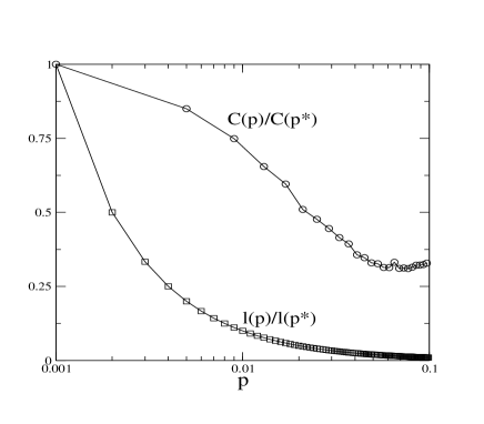
Figure 1: Normalized clustering coefficient ($\circ$) and average separation between node ($\square$) versus probability of non-local connections, with $N=100$ and $p^{*}=10^{-3}$.

We consider a network composed of $M$ small-world subnetworks with $L$ neurons each (Fig. 2). A given node has a probability $p_{i}$ to connect with other nodes inside the cluster, and a probability $p_{o}$ to be connected with neurons outside the cluster, the intercluster probability.

Figure 2: Schematic representation of $M=4$ one-dimensional small-world networks, each of $L=8$ nodes.

Neuron model: There are a number of mathematical models which emulate neuronal activity, ranging from differential equations hindmarsh to discrete-time maps rulkov . We choose the Rulkov model

$$x(n+1) = f(x(n),y(n))=\frac{\alpha}{1+[x(n)]^{2}}+y(n),$$ (1)

$$y(n+1) = g(x(n),y(n))=y(n)-\sigma x(n)-\beta,$$ (2)

where $x(n)$ is the fast and $y(n)$ is the slow dynamical variable. Furthermore, $\alpha$ affects directly the spiking time-scale and is chosen so that the time series of $x(n)$ presents an irregular sequence of spikes. The parameters $\sigma$ and $\beta$ describe the slow time-scale.

Phase Dynamics: We consider the neurons to be non-identical, that is, they possess a mismatch in their internal parameters, we choose $\alpha$ as a mismatch parameter. Complete synchronization in networks of non-identical neurons is not possible. However, weaker synchronization such as phase synchronization pikovsky may take place.

To study phase synchronization, we need to introduce a phase for the chaotic dynamics of the bursts. This turns out to be a non straightforward task. For chaotic oscillators the phase cannot be defined unambiguous. Different ways to introduce a phase are possible, each one being chosen according to the particular case studied josi ; pereira2 .

We consider the phase being increased by $2\pi$ at the beginning of each burst. We consider the burst to begin when the slow variable $y(n)$, which presents nearly regular saw-teeth oscillations, has a local maximum, in well-defined instants of time we call $t_{k}$. The duration of the chaotic burst, $t_{k+1}-t_{k}$, depends on the variable $x(n)$ and fluctuates in an irregular fashion as long as $x(n)$ undergoes chaotic evolution batista07 .

We can define a phase describing the time evolution within each burst, varying linearly from $t_{k}$ to $t_{k+1}$

$$\phi(t)=2\pi k+2\pi\frac{t-t_{k}}{t_{k+1}-t_{k}},\mbox{ }t_{k}\leq t<t_{k+1}$$ (3)

where $t_{k}$ denotes the time occurrence of the $k$th burst. The bursts occur in a coherent manner, that is, the time interval between burst have a small deviation.

Chemical Synapses: We analyze a neuron network coupled via excitatory synapse. We model the synapse as a static sigmoidal nonlinear input-output function with a threshold and a saturation parameters sompolinsky . We order the neurons within the network from $1,2,\ldots,ML$, and denote the dynamical variables of the $i$th neuron as $x_{i}(n)$ and $y_{i}(n)$.

The coupling function is given by

$$V(x_{i}(n),x_{j}(n))=(x_{i}(n)-V_{s})S(x_{j}(n)),$$

where (the reversal potential) $V_{s}>x_{i}(n)$ for any $x_{i}(n)$ implies that the synapse is excitatory. Here $V_{s}=2.0$. The synaptic coupling function $S$ is modeled by the sigmoidal function

$$S(x)=\frac{1}{1+e^{-\lambda(x-\Theta_{s})}}.$$ (4)

We take the saturation parameter $\lambda=10$, and the value of $\Theta_{s}=-0.25$ is chosen in such a way that every spike within a single neuron burst can reach the threshold.

The network dynamics is described by

$$x_{i}(n+1) = f(x_{i}(n),y_{i}(n))+\varepsilon\sum_{j=1}^{N}a_{ij}V(x_{i}(n),x_{j}(n)),$$

$$y_{i}(n+1) = g(x_{i}(n),y_{i}(n)),$$ (5)

where $i=1,2,...,ML$, $\sigma=\beta=0.001$, and $\alpha_{i}$ to be different for each node on uniform values deviate in the interval $[4.1,4.4]$. $\varepsilon>0$ is the overall coupling strength, and $A=(a_{ij})$ is the adjacency matrix, $a_{ij}$ is $1$ if neuron $i$ is connected to neuron $j$, and zero otherwise.

The local part of the interaction considers the nearest and the next-to-the-nearest neighbors of a given node. Moreover, with probability $p_{i}$ a new long range connection is created inside the each cluster, and with probability $p_{o}$ to create an outside connection.

III Global phase synchronization of bursting neurons

The collective behavior of the network may be captured by the network mean field.

$$\langle x\rangle_{\mu}(n)=\frac{1}{ML}\sum_{i=1}^{ML}x_{i}(n).$$

The emergence of a collective behavior enhances the mean field dynamics.

To illustrate the mean field dependence on the synchronization we choose $M=4$ and $L=100$ with $p_{i}=10^{-2}$, $p_{o}=10^{-3}$. For small values of the overall coupling parameter $\varepsilon=0.01$ the neurons burst in a nonsynchronized fashion. The mean field presents no dynamics, but a noise-like signal, fluctuating around the mean value Fig. 3(a).

The more synchronized neurons the higher the mean field. For a coupling $\varepsilon=0.04$ the mean field already captures the dynamics of the burst (slow time-scale) dynamics Fig. 3(b). For the chosen $p_{i}$ and $p_{o}$, if the coupling strength is large enough then the network globally burst phase synchronize. Close to global synchronization $\varepsilon=0.1$ the mean field already reveals the bursting dynamics, while the fast oscillation due to the spike are filtered, see Fig. 3(c). This shows that even though the burst are synchronized the spikes can remain out of synchrony.

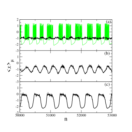
Figure 3: Behavior of the mean field as a function of the overall coupling parameter with fixed $p_{i}=10^{-2}$, $p_{o}=10^{-3}$, $M=4$ and $L=100$. a) $\varepsilon=0.01$ mean field presents no dynamics, but a noise-like behavior. b) $\varepsilon=0.04$ some neurons are synchronized and the mean field exhibit slows oscillators. c) $\varepsilon=0.1$ close to global synchronization the mean field shows the bursting dynamics.

The order parameter characterizes the emergence of synchrony in the network

$$z_{n}=R_{n}\exp(\rm{i}\Phi_{n})\equiv\frac{1}{N}\sum_{j=1}^{N}\exp(\rm{}i\phi_{n}^{(j)}),$$ (6)

where $R_{n}$ and $\Phi_{n}$ are the amplitude and angle, respectively, of a centroid phase vector for a one-dimensional network with periodic boundary conditions. If the bursting phases $\phi_{n}^{(j)}$ are spatially uncorrelated, their contribution to the result of the summation in Eq. (6) is small. However, in a globally phase synchronized state the order parameter magnitude asymptotes the unity.

The time averaged order parameter magnitude is given by

$${\bar{R}}=\frac{1}{T}\sum_{n=1}^{T}R_{n},$$

clearly depends on $\epsilon$ and both $p_{i}$, $p_{o}$ in and out connection probability. If the bursting dynamics is globally synchronized then $\overline{R}\approx 1$.

Our numerical analysis shows that clustered networks with good global synchronization properties is possible only for when a $p_{o}$ is larger than a certain critical value. This critical values clearly depends on the number of subnetworks. For a network that contains many clusters a larger $p_{o}$ is required to achieve global synchronization.

Fig. 4 shows the evolution of the average global order parameter $\bar{R}$ for fixed $p_{i}=10^{-2}$ and $L=100$. In Fig. 4 a) we have $M=2$ and b) $M=4$, where we depict the behavior of $\overline{R}$ for various values of the $p_{o}$. In the absence of outside connections and $\varepsilon$ large enough $\overline{R}\approx 1/M$, and if $p_{o}$ and $\varepsilon$ are large enough $\overline{R}\approx 1$. For $\varepsilon=0$ it must yield $\overline{R}\propto(ML)^{-1/2}$ so if $L\gg 1$ or $M\gg 1$ $\overline{R}$ must be close to zero.

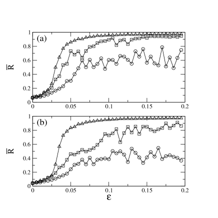
Figure 4: Time averaged order parameter as a function of the coupling strength for $p_{i}=10^{-2}$ and $L=100$ fixed. a) $M=2$ and b) $M=4$. In both figures we have $p_{o}=0$ ($\circ$), $p_{o}=1.6\times 10^{-4}$ ($\square$), $p_{o}=2\times 10^{-3}$ ($\triangle$).

The global synchronization is achieved when $\bar{R}=1$. However, if phase synchronization is achieved $\phi_{i}\approx\phi_{j}$ an almost global synchronized behavior can be obtain by setting a threshold value near 1, we choose $\bar{R}=0.95$. The minimum coupling strength necessary to achieve $\bar{R}=0.95$ is the critical coupling strength $\varepsilon_{c}$, the critical coupling parameter for global burst phase synchronization.

Phase Reduction: the application of the Kuramoto phase reduction techniques kuramoto ; liu leads to an approximate phase equation to describe the collective phase dynamics of the neuron ensemble. Since the burst dynamics is coherent. It is possible to introduce a coordinate change such that the phase of the i$th$ reads

$$\phi_{i}(t)=1+\psi_{i}(t)+\zeta_{i}(t),$$

where $\psi_{i}$ depends on the particular neuron and $\zeta$ is a small noise term josi .

Now, if the neurons are close to the onset of global synchronization $\phi_{j}\approx\phi_{i}$, the phase are described by $\psi_{i}$. Assuming that phase gradient is approximately constant along the trajectories, the phase reduction up to first order approximation renders

$$\dot{\psi}_{i}(t)=\omega_{i}+b\sum_{j=1}^{n}a_{ij}(\psi_{j}-\psi_{i}),$$

where $\omega_{i}$ depends on the neuron parameters and on the node degree. Close to the onset of synchronization $\psi_{j}-\psi_{i}\approx\sin(\psi_{j}-\psi_{i})$. So as a result the phase dynamics of the neuron network can be described (up to first order approximation) by the Kuramoto model

$$\dot{\phi}_{i}=\omega_{i}+\varepsilon\sum_{j=1}a_{ij}\sin(\phi_{j}-\phi_{i}),$$

where, $\varepsilon$ is a rescaled overall coupling strength and $a_{ij}$ is the adjacency matrix.

Recent results guan have given bounds for the critical coupling strength required for global synchronization to the probabilities of intracluster and intercluster connections. The critical coupling strength reads

$$\varepsilon_{c}=\frac{C}{p_{i}(L-1)+p_{o}(N-L)},$$ (7)

where the constant $C$ depends on the threshold value of the average global order parameter $\bar{R}$ for defining global synchronization, that can be regarded as a fitting parameter. Besides, a node is connected with $L-1$ nodes in the same cluster with probability $p_{i}$ that in our case is $L-5$, and the node is connected with $N-L$ nodes from different cluster with probability $p_{o}$. Thus, up to first order approximations, the onset of global bursting synchronization can be described in terms of Eq. (7)

Our detailed numerical analysis corroborates the theoretical prediction. In Fig. 5 $p_{i}=10^{-2}$ and $L=100$, furthermore we use $M=2$ in Fig. a) and $M=4$ Fig. b). In both figures the circles represent the critical values in accordance with the threshold global order parameter equal $0.95$. The solid curve is the theoretical prediction of the equation (7) with $\varepsilon_{c}+\delta$,

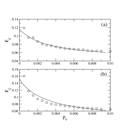
Figure 5: $\varepsilon_{c}$ versus $p_{o}$ for a network with $L=100$ and $p_{i}=10^{-2}$. The circles are for the threshold value of the global order parameter equal 0.95 and solid line $\varepsilon_{c}=C/[p_{i}(L-5)+p_{o}(N-L)]+\delta$, where (a) $M=2$, $C=0.07$ and $\delta=0.045$, and (b) $M=4$, $C=0.112$ and $\delta=0.032$.

The probability $p_{o}$ increases and the critical coupling strength required for global synchronization decreases. This shows that as the network become are homogeneous the global synchronization properties are enhanced.

IV Transition to phase synchrony

The transition to synchronization occurs in an intermittent fashion, where $\bar{R}$ has laminar phases. To analyze the intermittent behavior we introduce the quantity

$$F={1\over s}\sum_{1}^{s}N_{R}/\Delta_{n},$$

where $N_{R}$ is the number of occurrences of $\bar{R}>\xi$ ($\xi=0.95$) that we find within a time interval $\Delta_{n}$ and $s$ is the number of configurations of the connections distributed with the determined probability $p_{o}$. Thus, $F$ can be interpreted as the fraction of global synchronization in a given time interval.

$F$ depends on the coupling strength $\varepsilon$, and may present distinct behaviors as a function of the intercluster probability $p_{o}$. In Fig. 6(a) we depict the dependence of $F$ on $p_{o}$. The transition to global synchronization is abrupt for $p_{o}=10^{-1}$ and $\varepsilon_{c}\approx 0.05$, while it is not abrupt for $p_{o}=10^{-2}$ and $p_{o}=2\times 10^{-3}$.

Such behavior can be understood heuristically in terms of the synchronization properties of each isolated network. If $p_{o}$ is small enough, each network is almost independent. Hence, each network tend to synchronize by itself. So, as we increase the coupling each cluster synchronize and only then a behavior towards global synchronization is seen. This leads to a smooth transition. However, if $p_{o}$ is large then the collective dynamics of each subnetwork is strongly affected by the remaining subnetwork. So the synchronization occurs in one subnetwork is quickly spreads over the whole network, leading to a abrupt transition.

V Conclusions

In conclusion, we presented a neuronal clustered network model in which the neuron dynamical is described by the Rulkov map, furthermore the connective architecture presents the small-world property. We demonstrated the possibility of obtaining bursting global synchronization of Rulkov neurons in a clustered networks, where the probability of intercluster is varied and the clusters exhibit small-world property. Moreover, the network becomes more synchronizable when the probability of intercluster links is increased. That is, for a fixed $p_{i}$ the increasing of $p_{o}$, the out connection probability, enhances global synchronization. This means that when heterogeneity between the communities (clusters) is suppressed the network as a whole synchronizes better. The critical coupling parameter required for global synchronization as a function of the probability of intercluster presents the same behavior as Kuramoto-type dynamics.

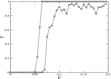
Figure 6: Fraction of time where the clustered network has larger ${\bar{R}}$ than 0.95 versus coupling strength. We consider a clustered network with $L=100$, $M=2$, $p_{i}=10^{-2}$, $s=20$, and $p_{o}=10^{-1}$ ($\circ$) and $p_{o}=10^{-2}$ $(\square)$. This two probabilities leads to distinct transitions to global synchronization.

References

- (1) G. Buzsaki, Rhythms of the Brain, Oxford University Press (2006).
- (2) E. Salinas and T. J. Sejnowski, Nature Neuroscience 2, 539 (2001).
- (3) E. Rodriguez, N. George, J. P. Lachaux, J. M. B. Renault and F. J. Varela, Nature 397, 430 (1999).
- (4) P. Fries, J. H. Reynolds, A. E. Rorie and R. Desimone, Science 29, 1560 (2001).
- (5) C. J. Stam and E. A. Bruin, Hum. Brain Mapp. 22, 97 (2004).
- (6) P. Hagmann, M. Kurant, X. Gigandet, P. Thiran, V. J. Wedeen, R. Mueli, and J. -Ph. Thiran, PLoS ONE 2(7) e597 (2007).
- (7) W. Schultz, J. Neurophysiol. 80, 1 (1998).
- (8) A. S. Freeman, L. T. Meltzer and B. S. Bunney, Life Sci. 36, 1983 (1985).
- (9) A. A. Grace and B. S. Bunney, Neuroscience 10, 2866 (1984).
- (10) M. Dhamala, V. K. Jirsa and M. Ding, Physical Review Letters 92, 028101, 1 (2004).
- (11) T. Pereira, M. S. Baptista and J. Kurths, European Physics Journal Special Topics 146, 155 (2007).
- (12) M. E. J. Newman and D. J. Watts, Physical Letters A 263, 341, 1 (1999).
- (13) A. M. Batista, S. E. de S. Pinto, R. L. Viana and S. R. Lopes, Physica A 322, 118 (2003).
- (14) J. L. Hindmarsh and R. M. Rose, Philosophical Transactions of the Royal Society London B 221, 87 (1984).
- (15) N. F. Rulkov, Physical Review Letters 86, 183 (2001).
- (16) A. S. Pikovsky, M. G. Rosenblum and J. Kurths, Cambridge University Press. Synchronization: A Universal Concept in Nonlinear Sciences (2001).
- (17) k. Josić and D. J. Mar, Physical Review E, 64, 056234, 1 (2001).
- (18) T. Pereira, M. S. Baptista and J. Kurths, Physics Letters A 362, 159 (2007).
- (19) C. A. S. Batista, A. M. Batista, J. A. C. de Pontes, R. L. Viana and S. R. Lopes, Physical Review E 76, 016218, 1 (2007).
- (20) H. Sompolinsky, A. Crisanti and H. J. Sommers, Physical Review Letters 61, 259 (1988).
- (21) Y. Kuramoto, Chemical Oscillations, Waves and Turbulence, Dover Pub. Inc. (2003).
- (22) C. Liu, D. R. Weaver, S. H. Strogatz and S. M. Reppert, S. M., Cell 91, 855 (1997).
- (23) S. Guan, X. Wang, Y.-C. Lai and C.-H Lai, Physical Review E 77, 046211, 1 (2008).