Dissipation-induced correlations in 1D bosonic systems

Abstract

The quantum dynamics of interacting bosons in a one-dimensional system is investigated numerically. We consider dissipative and conservative two-particle interactions, and integrate the master equation describing the system dynamics via a time-evolving block-decimation (TEBD) algorithm. Our numerical simulations directly apply to stationary-light polaritons in systems where atoms and photons are confined to the hollow core of a photonic crystal fibre. We show that a two-particle loss term can drive an initially uncorrelated state into a regime where correlations effectively inhibit the dissipation of particles. The correlations induced by two-particle losses are compared with those generated by an elastic repulsion. For the considered time range, we find a similar behaviour in local density-density correlations but differences in non-local correlations.

1 Introduction

The preparation of quantum systems in entangled many-body states is an indispensable resource for quantum information science [1] and allows one to access the rich physics of strongly correlated many-body systems [2]. Despite its reputation as the main adversary of quantum information schemes, dissipation was recognised recently as a versatile tool for the generation of specific many-body states [3, 4, 5].

The preparation of correlated quantum states via dissipation requires that the target state itself is metastable. An intriguing experiment [6] with cold molecules showed that a dissipative two-particle interaction between bosons in 1D gives rise to correlations that inhibit the loss of particles. The formal analysis of this effect is based on a generalised Lieb-Liniger model [7, 8, 9] and suggests that the two-particle loss term effectively results in a repulsion such that inelastic collisions between particles are avoided. In the limit of strong interactions [8], the two-particle losses give rise to a Tonks-Girardeau gas [10] where bosons behave with respect to many observables as if they were fermions.

Recently, it was shown that 1D systems of interacting bosons can be realised via dark-state polaritons that arise in light-matter interactions under conditions of electromagnetically induced transparency [11, 12, 13, 14, 15]. A possible experimental realisation of the polariton schemes is the setup described in [16, 17], where photons and atoms are simultaneously confined to the hollow core of a photonic-crystal fibre, see Fig. 1. Another approach comprises the experimental setup in [18], where atoms are trapped near the surface of an optical nanofibre using evanescent waves. The nature of the polariton-polariton interaction in these approaches can be tuned by external parameters and can be elastic [13] or dissipative [14, 15], and the interaction strength is maximal for a purely dissipative interaction [14]. Polariton schemes [13, 14, 15, 19, 20, 21] are extremely promising candidates for the realisation of strongly correlated photon states.

Here we consider bosons in 1D and investigate the quantum dynamics after a sudden switch-on of elastic and inelastic interactions via time-dependent density matrix renormalisation group techniques. The master equation of the system and the uncorrelated initial state are chosen such that our simulations directly apply to polariton systems [13, 14, 15]. All details of our model are discussed in Sec. 2, and numerical results are presented in Sec. 3. In particular, we are interested in the preparation of a correlated, non-decaying state via dissipative two-particle interactions that we discuss in Sec. 3.1. Non-local correlations are investigated in Sec. 3.2, where we show that dissipation and repulsion give rise to different results. Finally, a summary is provided in Sec. 4.

2 Model

We consider bosons of mass $m$ in a one-dimensional system of length $L$ that experience a two-particle contact interaction that can be either conservative, dissipative or a mixture of both. First we describe the full master equation governing the time evolution of the system in Sec. 2.1. A physical realisation of this model via interacting dark-state polaritons [14, 15] is introduced in Sec. 2.2. Finally, we discuss the discretised model of the master equation in Sec. 2.1 that allows us to perform numerical simulations in Sec. 2.3.

2.1 Master equation

The dynamics of bosons in our 1D system is described by the master equation

$$\hbar\partial_{t}\varrho=-iH_{\mathrm{eff}}\varrho+i\varrho H_{\mathrm{eff}}^{\dagger}+\mathcal{I}\varrho+\hbar\mathcal{L}_{\mathrm{D}}\varrho,$$ (1)

where $H_{\mathrm{eff}}$ is a non-hermitian Hamiltonian,

$$H_{\mathrm{eff}}=\frac{\hbar^{2}}{2m}\int_{0}^{L}\mathrm{d}z\partial_{z}\psi^{\dagger}\partial_{z}\psi+\frac{\tilde{g}}{2}\int_{0}^{L}\mathrm{d}z\psi^{\dagger 2}\psi^{2}.$$ (2)

Here $\psi(z)$ is the field operator obeying bosonic commutation relations

$$[\psi(z),\psi^{\dagger}(z^{\prime})]=\delta(z-z^{\prime}),$$ (3)

and the first term in Eq. (2) describes the kinetic energy. The parameter $\tilde{g}$ is the complex coupling constant and its real part gives rise to a hermitian contribution to $H_{\mathrm{eff}}$ in Eq. (2) that accounts for elastic two-particle collisions. On the other hand, the imaginary part of $\tilde{g}$ together with the term

$$\mathcal{I}\varrho=-\mathrm{Im}(\tilde{g})\int_{0}^{L}\mathrm{d}z\psi^{2}\varrho\psi^{\dagger 2}$$ (4)

in Eq. (1) constitutes a two-particle loss term that can be written in Lindblad form [22] as $\mathrm{Im}(\tilde{g}/2)\mathcal{D}[\psi^{2}]$, where $\mathcal{D}[\hat{X}]=\int_{0}^{L}\mathrm{d}z(\hat{X}^{\dagger}\hat{X}\varrho+\varrho\hat{X}^{\dagger}\hat{X}-2\hat{X}\varrho\hat{X}^{\dagger})$. The last term in Eq. (1) is defined as

$$\mathcal{L}_{\mathrm{D}}\varrho=-\frac{D}{2}\int_{0}^{L}\mathrm{d}z\mathcal{D}[\partial_{z}\psi]$$ (5)

and causes diffusion of the field $\psi$. Throughout this paper we choose

$$D=|\hbar/m|/10$$ (6)

such that the losses associated with the diffusion term are small on a timescale set by the kinetic energy term in Eq. (2).

The master equation (1) without the last term $\mathcal{L}_{\mathrm{D}}\varrho$ defined in Eq. (5) can be identified with the dissipative Lieb-Liniger model [8]. For a fixed number of particles $N_{\mathrm{ph}}$, essential features of the system are described by the complex Lieb-Liniger parameter

$$G=\frac{m\tilde{g}}{\hbar^{2}N_{\mathrm{ph}}/L}.$$ (7)

The spectrum of the effective Hamiltonian in Eq. (2) was analysed in [8] via the Bethe-Ansatz. It was found that the ground state of the so-called gaseous states (all momenta converge to finite values for $|G|\rightarrow\infty$) approaches the Tonks-Girardeau gas in the limit $|G|\rightarrow\infty$. This state is metastable since in the Tonks-Girardeau gas limit two particles never occupy the same position in space, and hence the two-particle contact interaction does not contribute to the dissipation of particles.

This feature can be formally derived from the master equation (1). The two-particle loss term $\mathrm{Im}(\tilde{g}/2)\mathcal{D}[\psi^{2}]$ in Eq. (1) causes a time dependence of the density of particles according to

$$\partial_{t}\langle\hat{n}(z)\rangle=\frac{2}{\hbar}\mathrm{Im}(\tilde{g})g^{(2)}(z,z)\langle\hat{n}(z)\rangle^{2},$$ (8)

where $\hat{n}(z)=\psi^{\dagger}(z)\psi(z)$ is the particle density operator and

$$g^{(2)}(z,z^{\prime})=\frac{\langle\psi^{\dagger}(z)\psi^{\dagger}(z^{\prime})\psi(z)\psi(z^{\prime})\rangle}{\langle\hat{n}(z)\rangle\langle\hat{n}(z^{\prime})\rangle}$$ (9)

is the second order correlation function. Note that the kinetic energy and the diffusion term $\mathcal{L}_{\mathrm{D}}\varrho$ in Eq. (1) will, in general, induce an additional time dependence of $\langle\hat{n}(z)\rangle$. The kinetic energy term conserves the total number of particles but gives rise to polariton fluxes from and to position $z$ that would redistribute the polariton density. In regions where the system and the particle density are homogeneous, these fluxes can safely be neglected. The impact of the diffusion term $\mathcal{L}_{\mathrm{D}}\varrho$ is negligible for the considered time scales since we chose a small value for the parameter $D$ in Eq. (6). In the strongly correlated regime and for a homogeneous system, the gaseous ground state of $H_{\mathrm{eff}}$ obeys [8]

$$g^{(2)}(z,z)=(1-1/N_{\mathrm{ph}}^{2})4\pi^{2}/(3|G|^{2}),$$ (10)

and hence $g^{(2)}(z,z)\ll 1$ for $|G|$ sufficiently large. The combination of Eqs. (8) and (10) implies that a purely dissipative interaction term supports metastable states.

2.2 Physical realisation

Figure 1: (a) Considered setup of $N_{\mathrm{a}}$ atoms confined to an interaction volume of length $L$ and transverse area $A$. $\Omega_{\pm}$ are the Rabi frequencies of the classical control fields, and $\hat{E}_{\pm}$ are the quantum probe fields. (b) Atomic level scheme. $\gamma_{ij}$ is the full decay rate on the $|i\rangle\leftrightarrow|j\rangle$ transition, $\delta$ and $\Delta$ label the detuning of the probe fields with states $|3\rangle$ and $|4\rangle$, respectively, and $\varepsilon$ is the two-photon detuning.

An example for a physical system that is described by the master equation (1) is shown in Fig. 1(a), where photons and atoms are simultaneously confined to the hollow core of a photonic-crystal fibre. Since the light-guiding core of the optical fibre is of the same order of magnitude as the optical wavelength, the fibre represents a one-dimensional waveguide for the optical fields. The level scheme of each atom inside the fibre is shown in Fig. 1(b). The dynamics of the system can be described in terms of dark-state polaritons [23] representing bosonic quasi-particles that arise in light-matter interactions under conditions of electromagnetically induced transparency (EIT) [24]. The two counter-propagating control fields $\Omega_{\pm}$ [see Fig. 1(a)] of equal intensity give rise to stationary light [25, 26] where the polaritons experience a quadratic dispersion relation like bosons in free space. Moreover, the coupling of the probe fields to the transition $|2\rangle\leftrightarrow|4\rangle$ induces a two-particle contact interaction between the polaritons that can be conservative [11, 13], dissipative or a mixture of both [14, 15]. It can be shown [14, 15] that the dark-state polariton dynamics can be described by the master equation (1), where the effective mass $m$ and the complex coupling constant $\tilde{g}$ depend on the detunings $\delta$, $\Delta$ [see Fig. 1(b)] and the intensity of the control fields. In particular, we point out that a proper adjustment of the detuning $\delta$ allows one to fulfil Eq. (6), and the choice of the detuning $\Delta$ determines the relative contribution of elastic and inelastic processes to the two-particle interaction.

In an experiment, the evolution of the polaritons under Eq. (1) has to be preceded by a loading process that could be realised as follows [13]. Initially the probe field modes are empty and only the control field $\Omega_{+}$ is switched on. Then a probe pulse copropagating with $\Omega_{+}$ enters the fibre under conditions of electromagnetically induced transparency. Here we assume that the transition $|4\rangle\leftrightarrow|2\rangle$ is far off-resonant during the loading process such that its influence is negligible. The dynamics of the probe field inside the medium can be described concisely in terms of dark-state polaritons [23]. As compared to the pulse propagating in vacuum, the polariton pulse inside the medium is spatially compressed and travels with a reduced group velocity $v_{g}\propto\Omega_{+}^{2}$. Once the pulse is entirely inside the fibre, the group velocity of the polariton pulse is reduced to zero by an adiabatic switch-off of the control field $\Omega_{+}$. The latter process maps the polaritons into a stationary spin coherence, and all probe field modes are empty. Eventually both control fields are switched on adiabatically and with equal intensity, $\Omega_{\pm}=\Omega_{0}$. The time evolution of the corresponding dark-state polaritons is then determined by the master equation (1) [14, 15]. Note that the adiabatic switch-on can be much faster than all typical timescales in the master equation (1). At this stage, the detuning $\Delta$ of the probe field with the $|4\rangle\leftrightarrow|2\rangle$ transition can be adjusted by a proper choice of the frequency of the counterpropagating control fields. This frequency can be different from the one used for the single control field during the loading process.

The correlations that built up under the evolution of the master equation (1) can be measured if the intensity of the control field $\Omega_{-}$ is reduced. The latter process converts the stationary polaritons into a propagating pulse with controllable group velocity. This procedure maps spatial correlations of the trapped pulse into temporal correlations of the output light that can be detected via standard quantum optical techniques.

2.3 Discretised model

The dynamics of the system is studied via the time-evolving block decimation algorithm [27, 28, 29] for density operators. The discretised version [30] of Eq. (1) is given by a generalised Bose-Hubbard model augmented by loss terms,

$$\dot{\varrho}=-\frac{i}{\hbar}[H_{1}+H_{2},\varrho]+\mathcal{L}_{1}\varrho+\mathcal{L}_{2}\varrho.$$ (11)

Here $H_{1}$ and $H_{2}$ correspond to the kinetic energy term and the conservative contribution to the two-particle interaction, respectively,

$$H_{1}=2J\sum\limits_{l}\hat{a}^{\dagger}_{l}\hat{a}_{l}-J\sum\limits_{l}(\hat{a}_{l}\hat{a}^{\dagger}_{l+1}+\hat{a}_{l+1}\hat{a}^{\dagger}_{l}),\qquad H_{2}=\frac{U}{2}\sum\limits_{l}\hat{a}_{l}^{\dagger 2}\hat{a}_{l}^{2},$$ (12)

and $J$ and $U$ are defined as

$$J=\frac{\hbar^{2}}{2m}\frac{1}{\Delta z^{2}},\qquad U=\mathrm{Re}(\tilde{g})\frac{1}{\Delta z}.\\$$ (13)

The parameter $\Delta z$ is the lattice constant of the discretisation grid. The terms $\mathcal{L}_{1}\varrho$ and $\mathcal{L}_{2}\varrho$ in Eq. (1) are the discretised versions of the diffusion term in Eq. (5) and the dissipative contribution to the two-particle interaction, respectively,

$$\mathcal{L}_{1}\varrho= -\Gamma_{1}\sum\limits_{l}(\hat{a}_{l}^{\dagger}\hat{a}_{l}\varrho+\varrho\hat{a}_{l}^{\dagger}\hat{a}_{l}-2\hat{a}_{l}\varrho\hat{a}_{l}^{\dagger})$$

$$+\frac{\Gamma_{1}}{2}\sum\limits_{l}(\hat{a}_{l}^{\dagger}\hat{a}_{l+1}\varrho+\varrho\hat{a}_{l}^{\dagger}\hat{a}_{l+1}-2\hat{a}_{l+1}\varrho\hat{a}_{l}^{\dagger})$$

$$+\frac{\Gamma_{1}}{2}\sum\limits_{l}(\hat{a}_{l}\hat{a}_{l+1}^{\dagger}\varrho+\varrho\hat{a}_{l}\hat{a}_{l+1}^{\dagger}-2\hat{a}_{l}\varrho\hat{a}_{l+1}^{\dagger}),$$

$$\mathcal{L}_{2}\varrho=-\frac{\Gamma_{2}}{2}\sum\limits_{l}(\hat{a}_{l}^{\dagger 2}\hat{a}_{l}^{2}\varrho+\varrho\hat{a}_{l}^{\dagger 2}\hat{a}_{l}^{2}-2\hat{a}_{l}^{2}\varrho\hat{a}_{l}^{\dagger 2}),$$ (15)

and

$$\Gamma_{1}=D\frac{1}{\Delta z^{2}},\qquad\Gamma_{2}=-\mathrm{Im}(\tilde{g}/\hbar)\frac{1}{\Delta z}.$$ (16)

The discretised version Eq. (11) is a good approximation of the continuous master equation (1) if the smallest wavelength $\lambda_{\mathrm{min}}$ involved is much larger than the grid spacing $\Delta z$. Initially $\lambda_{\mathrm{min}}$ is determined by the momentum components of the initial state, but the evolution under Eq. (11) will change the momentum distribution of the sample. In particular, the suddenly switched-on two-particle repulsion term leads (among other processes) to a population of higher momentum states. It was found [31] that the lattice model is a good approximation provided that $U/J\ll 1$. If the latter inequality is violated, lattice artefacts occur. We find that these effects do not occur for a purely dissipative two-particle interaction ($U=0$) even if $\hbar\Gamma_{2}/J\approx 1$.

For all numerical simulations we consider a grid with $N_{\mathrm{s}}=500$ sites, and the physical state space at each site $l$ is spanned by the four Fock states $\{|0\rangle_{l},|1\rangle_{l},|2\rangle_{l},|3\rangle_{l}\}$ allowing for a maximum occupation of three particles at each site. We verified the convergence of our algorithm by varying the bond dimension $\chi$ of the matrix product state. In our simulations, the truncation errors $\epsilon_{\mathrm{trunc}}$ are bounded by $\epsilon_{\mathrm{trunc}}\leq 10^{-4}$ for $\chi=100$.

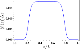
Figure 2: Spatial density distribution $\langle\hat{n}(z)\rangle$ of the initial state in Eq. (17).

The choice of the initial state for the numerical integration is motivated by the loading process of an optical pulse into the fibre as described in Sec. 2.2. We consider an initial state with a mean number of $\langle\hat{N}\rangle_{0}=5$ particles and a spatial density distribution as shown in Fig. 2. Here we neglect distortions and correlations due to the optical nonlinearity that may build up during the loading process. The initial shape of the polariton pulse is then determined by the slowly varying envelope of the probe pulse entering the system [23]. Furthermore, we assume that the initial polariton pulse is derived from laser light and thus described by a product of coherent states. In the discretised model we thus model the initial state by a coherent state at each site,

$$|\psi\rangle_{0}=\prod\limits_{l}\exp(-|c_{l}|^{2}/2)\exp(c_{l}a_{l}^{\dagger})|0\rangle,$$ (17)

where $\sum_{l}|c_{l}|^{2}=5$ and $|c_{l}|^{2}=\Delta z\langle\hat{n}(z_{l})\rangle$ with $z_{l}=l\Delta z$. We point out that $|\psi\rangle_{0}$ in Eq. (17) is an uncorrelated state with $g^{(2)}(z,z^{\prime})=1$ for all values of $z,z^{\prime}$ in the sample.

3 Numerical results

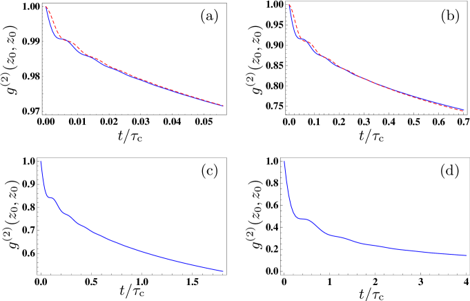
Figure 3: Temporal evolution of $g^{(2)}(z_{0},z_{0})$ at the centre $z_{0}=L/2$ of the sample for (a) $|G|=1$, (b) $|G|=10$, (c) $|G|=20$ and (d) $|G|=100$. The timescale $\tau_{\mathrm{c}}$ is defined in Eq. (19), and the solid lines correspond to a purely dissipative two-particle interaction, $\mathrm{Re}(\tilde{g})=0$. In (a) and (b), the dashed line shows the result for an interaction that is predominantly repulsive [$|\mathrm{Re}(\tilde{g})/\mathrm{Im}(\tilde{g})|=10$].

Next we describe the results of the numerical integration of the master equation (11). Starting from the initial state in Eq. (17), the interaction is suddenly switched on at $t=0$. We consider various scenarios where the interaction is purely dissipative or predominantly conservative. In Sec. 3.1, we discuss whether two-particle losses alone are able to drive the system into a correlated regime where dissipation of particles is suppressed. As discussed in Sec. 2.1, the inhibition of two-particle losses is linked to local correlations in the sample. The second part Sec. 3.2 is concerned with non-local correlations. In particular, we compare non-local correlations created by a purely dissipative and a predominantly conservative interaction.

3.1 Inhibition of two-particle losses

The two-particle decay term in Eq. (1) in general leads to a loss of particles from the system. The rate at which the particle density diminishes is determined by Eq. (8) and depends crucially on the local correlations $g^{(2)}(z,z)$ of the system. Figure 3 shows the temporal evolution of $g^{(2)}(z_{0},z_{0})$ at the centre $z_{0}=L/2$ of the sample for different values of the Lieb-Liniger parameter $|G|$ according to the numerical integration of Eq. (11). The values of $|G|$ correspond to the mean particle number $\langle\hat{N}\rangle_{0}=5$ of the initial state, see Eq. (17). All solid lined lines in Fig. 3 belong to a purely dissipative two-particle interaction, $\mathrm{Re}(\tilde{g})=0$. On the contrary, the dashed lines in Fig. 3 (a) and (b) correspond to a predominantly conservative interaction $|\mathrm{Re}(\tilde{g})/\mathrm{Im}(\tilde{g})|=10$.

In the case of a purely conservative interaction ($\mathrm{Im}(\tilde{g})=0$), it was shown [31] that local quantities reach a stationary state on a timescale $T_{\mathrm{loc}}=\hbar/(\tilde{g}\rho)$, where $\rho=N_{\mathrm{ph}}/L$ is the density of particles. Note that the Lieb-Liniger gas does not thermalize globally [32]. Here we generalise this definition to the case of complex $\tilde{g}$ and define

$$T_{\mathrm{loc}}=\frac{\hbar}{|\tilde{g}|\rho}=\frac{m}{\hbar}\frac{1}{|G|\rho^{2}}.$$ (18)

Due to the enhanced numerical complexity of TEBD for density operators and numerical limitations, our simulations cannot cover the full time range $T_{\mathrm{loc}}$. In the following we scale time in the presentation of numerical results with

$$\tau_{\mathrm{c}}=2\frac{\hbar}{\sqrt{U^{2}+(\hbar\Gamma_{2})^{2}}}=\frac{1}{50}T_{\mathrm{loc}}.$$ (19)

The comparison between the dashed and solid lines in Figs. 3 (a) and (b) shows that dissipative and repulsive two-particle interactions are equally effective in the repulsion of particles on a timescale proportional to the inverse interaction strength $|\tilde{g}|$. Note that for the polariton system discussed in Sec. 2.2, $|\tilde{g}|$ is at least one magnitude larger for a purely dissipative interaction [14, 15] as compared to the conservative case. It follows that small values of $g^{(2)}(z_{0},z_{0})$ are reached much faster in absolute time for a dissipative two-particle interaction.

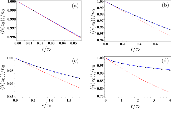
Figure 4: Temporal evolution of $\langle\hat{n}(z)\rangle$ at the centre $z_{0}=L/2$ of the sample for (a) $|G|=1$, (b) $|G|=10$, (c) $|G|=20$, (d) $|G|=100$. In (a)-(d), the solid line corresponds to a numerical integration of Eq. (8) with $g^{(2)}(z_{0},z_{0})$ taken from the TEBD simulation for a purely dissipative two-particle interaction, $\mathrm{Re}(\tilde{g})=0$. The dotted lines indicate the results of the TEBD simulation for $\langle\hat{n}(z)\rangle$. The dashed line shows the evolution of $\langle\hat{n}(z)\rangle$ according to Eq. (8) with $g^{(2)}(z_{0},z_{0})=1$ for all times.

We emphasise that the minimal values for $g^{(2)}(z_{0},z_{0})$ in Fig. 3 will decrease further in time until their equilibrium values are reached. An estimate of these equilibrium values can be obtained via the work presented in [31]. Here the authors performed TEBD simulations for the unitary time evolution of bosons in 1D with two-particle repulsion. In particular, this system could be described by a pure quantum state which reduces the numerical complexity as compared to our simulations of the full density operator. Therefore, the simulations in [31] could be carried out up to times $t=T_{\mathrm{loc}}$. Given that the initial dynamics of $g^{(2)}(z_{0},z_{0})$ for two-particle losses and for conservative interactions is very similar, one may suppose that the equilibrium values of $g^{(2)}(z_{0},z_{0})$ will also be almost the same. For this case we estimate that $g^{(2)}(z_{0},z_{0})$ for our system should lie within the range $[0.1,0.2]$ for $|G|=10$ and $|G|=20$ at $t=T_{\mathrm{loc}}$.

Next we determine the temporal evolution of the particle density at the centre of the cloud via Eq. (8) and the numerical results for the temporal evolution of $g^{(2)}(z_{0},z_{0})$. The result is represented by the solid lines in Fig. 4 and in good agreement with the direct evaluation of the particle density $\langle\hat{n}(z)\rangle$ via the numerical integration of the master equation (11) (dotted lines). The small deviations are due to the diffusion term in Eq. (5) that results in particle losses and that were omitted in Eq. (8). Note that all curves in Fig. 4 correspond to a purely dissipative two-particle interaction, $\mathrm{Re}(\tilde{g})=0$. In order to visualise the slowdown of two-particle losses due to the decrease of $g^{(2)}(z_{0},z_{0})$ in time, the dashed line in Fig. 4 shows the temporal evolution of $\langle\hat{n}(z)\rangle$ according to Eq. (8) with $g^{(2)}(z_{0},z_{0})=1$ for all times. The slowdown of two-particle losses is most pronounced for $|G|=100$ where a quasi-stationary regime is reached with $g^{(2)}(z_{0},z_{0})$ close to zero. We find that the decrease of the mean number of particles $\langle\hat{N}\rangle/\langle\hat{N}\rangle_{0}$ follows the same curves as the particle density at the centre of the cloud. It follows that more than $90\%$ of the initially present particles are left at $t/\tau_{\mathrm{c}}=4$ for $|G|=100$. Figures 4 (b) and (c) correspond to $|G|=10$ and $|G|=20$, respectively, and demonstrate a clear slowdown of two-particle losses. On the basis of the estimates for the equilibrium values of $g^{(2)}(z_{0},z_{0})$ obtained via the results presented in [31], we suppose that $50\%$ ($60\%$) of the initial particles are still present at $t=T_{\mathrm{loc}}$ for $|G|=10$ ($|G|=20$). On the contrary, $g^{(2)}(z_{0},z_{0})$ will not drop to values close to zero for $|G|=1$ and hence we expect that a significant number of particles is lost at $t=T_{\mathrm{loc}}$.

3.2 Non-local correlations

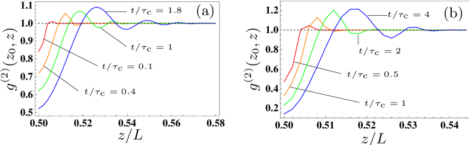
Figure 5: Spatial dependence of $g^{(2)}(z_{0},z)$ for a purely dissipative two-particle interaction [$\mathrm{Re}(\tilde{g})=0$]. The parameters correspond to (a) $|G|=20$ and (b) $|G|=100$, and $z_{0}=L/2$ is the centre of the sample.

The spatial dependence of $g^{(2)}(z_{0},z)$ as a function of $z$ ($z_{0}=L/2$ is the centre of the sample) is depicted in Fig. 5. Several snapshots in time are shown indicating that non-local correlations exhibit oscillations that propagate outwards. The oscillations for the longest evolution times in Fig. 5 exhibit several minima that lie below unity. It follows that a dissipative two-particle interaction alone to some extend gives rise to spatial order of the particles. Note that non-local correlations reach a quasi-stationary regime on a timescale that is much larger than $T_{\mathrm{loc}}$. In particular, we point out that the correlations shown in Fig. 6 are not Friedel oscillations [2] that characterise the Fermionic nature of particles in the Tonks-Girardeau regime.

In Sec. 3.1 we concluded that repulsion and dissipation are equally effective in the creation of small values of $g^{(2)}(z,z)$. On the other hand, dissipative and conservative two-particle interactions give rise to different non-local correlations as shown in Fig. 6. The solid and dashed lines correspond to a purely dissipative and a mostly conservative two-particle interaction, respectively. It can be seen that the non-local correlations propagate at the same velocity in space in the dissipative and conservative case, but the oscillations are more pronounced for a repulsive two-particle interaction. In addition, two-particle losses give rise to a broader dip in $g^{(2)}(z_{0},z)$ as a function of $z$ as compared to the conservative case. Note that the oscillation amplitudes in $g^{(2)}(z_{0},z)$ are also damped by the diffusion term in Eq. (5).

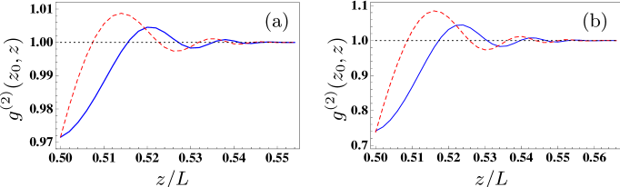
Figure 6: Spatial dependence of $g^{(2)}(z_{0},z)$ for (a) $|G|=1$, $t/\tau_{c}=0.056$ and (b) $|G|=10$, $t/\tau_{c}=0.77$. $z_{0}=L/2$ is the centre of the sample. The solid lines correspond to a purely dissipative two-particle interaction [$\mathrm{Re}(\tilde{g})=0$], and the dashed lines show the result for an interaction that is predominantly repulsive [$|\mathrm{Re}(\tilde{g})/\mathrm{Im}(\tilde{g})|=10$].

4 Discussion and summary

In this paper we investigated the quantum dynamics of bosons in 1D after a sudden switch-on of two-particle losses. The master equation and the uncorrelated initial state are chosen such that our simulations directly apply to stationary-light polariton systems [13, 14, 15]. Apart from a (small) diffusion term, the considered master equation coincides with the dissipative Lieb-Liniger model [8]. In particular, we investigated the dissipation-induced preparation of correlations that effectively inhibit two-particle losses. We found that a metastable regime where losses are substantially suppressed can be prepared for large values of the Lieb-Liniger parameter $|G|\gg 1$. Formally, it was shown [7, 8] that the two-particle loss term effectively results in a repulsion between particles such that they never occupy the same position in space. Therefore, dissipation via the two-particle contact interaction is inhibited. A physical explanation for this counterintuitive result can be given for a discrete lattice model [6, 7]. There it can be regarded as a manifestation of the quantum Zeno effect, where the two-particle losses play the role of a continuous measurement that always projects the system onto states with less than two particles in each lattice site before higher particle numbers can build up. Furthermore, we compared the correlations induced by dissipative and repulsive interactions, respectively. We found that dissipation and repulsion are equally efficient for the generation of local correlations $g^{(2)}(z,z)\leq 1$ on a timescale proportional to the inverse interaction strength. On the other hand, non-local correlations induced by dissipation show different features than those created by two-particle repulsion. As compared to an elastic repulsion between the particles, we find that two-particle losses give rise to a broader dip in $g^{(2)}(z_{0},z)$ as a function of $z$ ($z_{0}$ is the centre of the sample). Both repulsion and dissipation give rise to spatial oscillations in $g^{(2)}(z_{0},z)$ that spread in time and indicate to some extend a spatial ordering. We find that these oscillations are more pronounced for a repulsion between the particles as compared to the dissipative case.

References

References

- [1] M. A. Nielsen and I. L. Chuang. Quantum Computation and Quantum Information. Cambridge University Press, Cambridge, 2000.
- [2] I. Bloch, J. Dalibard, and W. Zwerger. Many-body physics with ultracold gases. Rev. Mod. Phys., 80:885, 2008.
- [3] B. Kraus, H. P. Bücheler, S. Diehl, A. Kantian, A. Micheli, and P. Zoller. Preparation of entangled states by quantum markov processes. Phys. Rev. A, 78:042307, 2008.
- [4] F. Verstraete, M. M. Wolf, and J. I. Cirac. Quantum computation and quantum-state engineering driven by dissipation. Nat. Phys., 5:633, 2009.
- [5] S. Diehl, A. Micheli, A. Kantian, B. Kraus, H. P. Bücheler, and P. Zoller. Quantum states and phases in driven open quantum systems with cold atoms. Nat. Phys., 4:878, 2008.
- [6] N. Syassen, D. M. Bauer, M. Lettner, T. Volz, D. Dietze, J. J. García-Ripoll, J. I. Cirac, G. Rempe, and S. Dürr. Strong dissipation inhibits losses and induces correlations in cold molecular gases. Science, 320:1329, 2008.
- [7] J. J. García-Ripoll, S. Dürr, N. Syassen, D. M. Bauer, M. Lettner, G. Rempe, and J. I. Cirac. Dissipation-induced hard-core boson gas in an optical lattice. New. J. Phys., 11:013053, 2009.
- [8] S. Dürr, J. J. García-Ripoll, N. Syassen, D. M. Bauer, M. Lettner, J. I. Cirac, and G. Rempe. Lieb-liniger model of a dissipation-induced tonks-girardeau gas. Phys. Rev. A, 79:023614, 2009.
- [9] S. K. Baur and E. J. Mueller. Two-body recombination in a quantum-mechanical lattice gas: Entropy generation and probing of short-range magnetic correlations. Phys. Rev. A, 82:023626, 2010.
- [10] M. Girardeau. Relationship between systems of impenetrable bosons and fermions in one dimension. J. Math. Phys., 1:516, 1960.
- [11] A. André, M. Bajcsy, A. S. Zibrov, and M. D. Lukin. Nonlinear optics with stationary pulses of light. Phys. Rev. Lett., 94:063902, 2005.
- [12] M. J. Hartmann, F. G. S. L. Brandão, and M. B. Plenio. Strongly interacting polaritons in arrays coupled cavities. Nat. Phys., 2:849, 2006.
- [13] D. E. Chang, V. Gritsev, G. Morigi, V. Vuletić, M. D. Lukin, and E. A. Demler. Crystallization of strongly interacting photons in a nonlinear optical fibre. Nat. Phys., 4:884, 2008.
- [14] M. Kiffner and M. J. Hartmann. Dissipation-induced tonks-girardeau gas of polaritons. Phys. Rev. A, 81:021806(R), 2010.
- [15] M. Kiffner and M. J. Hartmann. Master equation approach for interacting slow- and stationary-light polaritons. Phys. Rev. A, 82:033813, 2010.
- [16] M. Bajcsy, S. Hofferberth, V. Balic, T. Peyronel, M. Hafezi, A. S. Zibrov, V. Vuletic, and M. D. Lukin. Efficient all-optical switching using slow light within a hollow fiber. Phys. Rev. Lett., 102:203902, 2009.
- [17] S. Vorrath, S. A. Möller, P. Windpassinger, K. Bongs, and K. Sengstock. Efficient guiding of cold atoms through a photonic band gap fiber. New. J. Phys., 12:123015, 2010.
- [18] E. Vetsch, D. Reitz, G. Sagué, R. Schmidt, S. T. Dawkins, and A. Rauschenbeutel. Optical interface created by laser-cooled atoms trapped in the evanescent field surrounding an optical nanofiber. Phys. Rev. Lett., 104:203603, 2010.
- [19] Michael J. Hartmann. Polariton crystallization in driven arrays of lossy nonlinear resonators. Phys. Rev. Lett., 104(11):113601, 2010.
- [20] M. Leib and M. J. Hartmann. Bose–hubbard dynamics of polaritons in a chain of circuit quantum electrodynamics cavities. New. J. Phys., 12:093031, 2010.
- [21] M. Hafezi, D. E. Chang, V. Gritsev, E. Demler, and M. Lukin, arXiv:0907.5206v2 (2009).
- [22] H.-P. Breuer and F. Petruccione. The Theory of Open Quantum Systems. Oxford University Press, Oxford, 2006.
- [23] M. Fleischhauer and M. D. Lukin. Dark-state polaritons in electromagnetically induced transparency. Phys. Rev. Lett., 84:5094, 2000.
- [24] M. Fleischhauer, A. Imamoǧlu, and J. P. Marangos. Electromagnetically induced transparency: Optics in coherent media. Rev. Mod. Phys., 77:633, 2005.
- [25] A. André and M. D. Lukin. Manipulating light pulses via dynamically controlled photonic band gap. Phys. Rev. Lett., 89:143602, 2002.
- [26] M. Bajcsy, A. S. Zibrov, and M. D. Lukin. Stationary pulses of light in an atomic medium. Nature, 426:638, 2003.
- [27] M. Zwolak and G. Vidal. Mixed-state dynamics in one-dimensional quantum lattice systems; a time-dependent superoperator renormalization algorithm. Phys. Rev. Lett., 93:207205, 2004.
- [28] F. Verstraete, J. J. García-Ripoll, and J. I. Cirac. Matrix product density operators: simulation of finite-temperature and dissipative systems. Phys. Rev. Lett., 93:207204, 2004.
- [29] Michael J. Hartmann, Javier Prior, Stephen R. Clark, and Martin B. Plenio. Density matrix renormalization group in the heisenberg picture. Phys. Rev. Lett., 102:057202, 2009.
- [30] B. Schmidt, L. I. Plimak, and M. Fleischhauer. Stochastic simulation of a finite-temperature one-dimensional bose gas: From the bogoliubov to the tonks-girardeau regime. Phys. Rev. A, 71:041601(R), 2005.
- [31] D. Muth, B. Schmidt, and M. Fleischhauer. Fermionization dynamics of a strongly interacting 1d bose gas after an interaction quench. New. J. Phys., 12:083065, 2010.
- [32] T. Kinoshita, T. Wenger, and D. S. Weiss. A quantum newton’s cradle. Nature, 440:900, 2006.