Optimization of electron pumping by harmonic mixing

Abstract

For a symmetric bridge coupled to infinite leads, in the presence of a dipole-coupled external ac-field with harmonic mixing, we solve the Schrödinger equation in the time-domain using open boundary conditions as well as in the energy-domain using Floquet scattering theory. As this potential breaks parity and generalized parity, we find a non-vanishing average current. We then optimize the relative amplitude ratio between the fundamental and the second harmonic leading to a maximum in the pump current.

I Introduction

Generating non-vanishing average electronic currents in statically unbiased systems, i.e. electron pumping, by external ac-fields has been realized in experiments with quantum dots Switkes et al. (1999); DiCarlo and Marcus (2003); Vavilov et al. (2005), nanotubes Leek et al. (2005), semiconductor heterostructures Linke et al. (1999, 2002) and a Josephson junction array Majer et al. (2003).

Theoretically, the adiabatic case of slow driving has been treated amongst others by Thouless Thouless (1983), by Brouwer Brouwer (1998), who used a scattering approach, and by Zhou et al. Zhou et al. (1999), applying Keldysh-Green’s function methodology. The non-adiabatic, time-periodic case can be handled in the Floquet formalism, formally treating the system as time-independent. An early example of a similar strategy is the heuristic approach to understand the effect of time-periodic driving on the current voltage characteristics of superconductor-insulator-superconductor junctions that has been given by Tien and Gordon Tien and Gordon (1963). More recently, Floquet scattering theory has been used to get expressions for transmission probabilities Büttiker and Landauer (1982); Li and Reichl (1999); Tang and Chu (1999); Li and Reichl (2000); Martinez and Reichl (2001); Zhou and Li (2005); Emmanouilidou and Reichl (2002). In addition, Kim Kim (2002) as well as Moskalets and Büttiker Moskalets and Büttiker (2002) exploited this method for considering an electronic pump consisting of two oscillating $\delta$-peaks. In Büttiker and Landauer (1982); Li and Reichl (1999); Tang and Chu (1999); Li and Reichl (2000); Zhou and Li (2005); Kim (2002); Moskalets and Büttiker (2002); Emmanouilidou and Reichl (2002) the scattering matrix is determined from the matching conditions of the wave function. Furthermore, electron-pumping scenarios have been treated with the help of Floquet theory using an equation-of-motion approach in the Heisenberg picture Camalet et al. (2003); Kohler et al. (2005), solving the master equation Lehmann et al. (2003); Goychuk and Hänggi (1998); Kohler et al. (2005), or using non-equilibrium Green’s functions Stafford and Wingreen (1996); Arrachea (2005); Arrachea and Moskalets (2006). The authors of Camalet et al. (2003); Kohler et al. (2005); Lehmann et al. (2003); Goychuk and Hänggi (1998); Arrachea (2005) have considered tight-binding Hamiltonians, while in Stafford and Wingreen (1996) an interacting two-level system has been studied. Arrachea and Moskalets (2006) provides a comparison of Green’s function theory with the scattering matrix.

Recently, Kurth and coworkers Kurth et al. (2005) proposed a time-dependent approach for quantum transport, treating the leads by using open boundaries for the central region. This method is not restricted to time-periodic problems. In the same Reference a simple scheme for ac-transport is studied as one application. Stefanucci et al. Stefanucci et al. (2008) later used this algorithm of time-evolution for the investigation of systems where a net current is generated by a traveling wave in the potential of the Schrödinger equation.

In this paper, we consider a harmonic-mixing dipole field as another potential that shows the pumping effect. In order to break (generalized) parity, the external field is composed of a fundamental frequency component together with an additional second harmonic term. Harmonic mixing has been studied previously in the tight-binding case Kohler et al. (2005); Goychuk and Hänggi (1998) as well as purely classically Hänggi and Marchesoni (2009). In Section II, in order to calculate the transport across a structure under the influence of the external ac-field, we first review Floquet scattering theory, allowing us to arrive at an expression for the stationary net current from the matching conditions via the scattering matrix.

Secondly, in Section III, we treat the transport problem from a time-dependent point of view, focusing on the transient dynamics of the current after a sudden switching on of the driving. To this end we are considering the zero temperature case and are choosing an equilibrium state of the undriven system as initial condition Cini (1980). We review the algorithm of time-evolution from Ref. Kurth et al. (2005), where an expression for the time-dependent current is gained by using a Schrödinger equation with open boundaries. In Section IV we explicitly apply both ways to calculate the current in the problem of electron pumping and it is shown that the time-average of the current over one period converges in the long-time limit to the result of Floquet theory. That was to be expected as there are no bound states in the considered system which could lead to a non-convergent time dependence as shown in the work of Khosravi et al. Khosravi et al. (2009). Our studies extend previous work in the monochromatic case by Li and Reichl Li and Reichl (2000) and lead to optimal values for the relative amplitudes of the first and second harmonic as a function of the incoming energy. In Section V we give conclusions and an outlook.

II Floquet scattering theory

Floquet scattering theory has been employed to calculate transmission probabilities in tunneling systems driven by a monochromatic laser field Li and Reichl (1999); Henseler et al. (2001). Here we briefly review the formalism in order to apply it to the phenomenon of electron pumping.

We consider the time-dependent Schrödinger equation (TDSE) with one dimension in space (atomic units (a.u.) are used throughout the paper),

$$i\partial_{t}\Psi(x,t)=\left[-\frac{1}{2}\partial_{x}^{2}+V(x,t)\right]\Psi(x,t).$$ (1)

The potential shall fulfill the following conditions:

1. $V(x,t+T)=V(x,t)$ (periodicity in time),

2. there are $x_{L}<x_{R}\in\mathbb{R}$ with $V(x,t)=0~{}\text{if}~{}x<x_{L}~{}\text{or if}~{}x>x_{R}$,

3. within $x_{L}<x<x_{R}$ we know the analytical solution of the TDSE,

4. the potential is bounded.

We denote the left lead ($x<x_{L}$) with $L$, the right one ($x>x_{R}$) with $R$, and the central region ($x_{L}<x<x_{R}$) with $C$. Due to the time periodicity, i.e. condition 1 above, solutions of the TDSE can be written in the form Kohler et al. (2005)

$$\Psi(x,t) = e^{-i\epsilon t}\phi(x,t),$$ (2)

$$\phi(x,t+T) = \phi(x,t)=\sum_{n=-\infty}^{\infty}c_{n}(x)e^{-in\omega t},$$ (3)

where $\epsilon$ denotes the so called Floquet energy or quasi-energy, the frequency $\omega$ is given by $\omega=2\pi/T$.

The second condition for $V(x,t)$ leads to the following form of the solution in the region $x<x_{L}$,

$$\Psi(x,t)=e^{-i\epsilon t}\sum_{n=-\infty}^{\infty}\left(\frac{a_{L}^{n}}{\sqrt{k_{n}}}e^{ik_{n}x}+\frac{b_{L}^{n}}{\sqrt{k_{n}}}e^{-ik_{n}x}\right)e^{-in\omega t}$$ (4)

and for $x>x_{R}$,

$$\Psi(x,t)=e^{-i\epsilon t}\sum_{n=-\infty}^{\infty}\left(\frac{a_{R}^{n}}{\sqrt{k_{n}}}e^{-ik_{n}x}+\frac{b_{R}^{n}}{\sqrt{k_{n}}}e^{ik_{n}x}\right)e^{-in\omega t}$$ (5)

with the wavenumbers

$$k_{n}=\sqrt{2(\epsilon+n\omega)}.$$ (6)

The Floquet scattering matrix $S$ connects the outgoing current amplitudes $b_{\alpha}^{n}$ with the ingoing ones $a_{\alpha}^{n}$:

$$b_{\alpha}^{n}=\sum_{\beta=L,R}\sum_{m}S_{\alpha\beta}^{nm}a_{\beta}^{m}.$$ (7)

To quantify the net current $\langle I\rangle=1/T\int_{0}^{T}{\rm d}t~{}I(t)$, we have to include a summation over the Floquet modes in the Landauer formula Moskalets and Büttiker (2002) as an incoming wave with energy $E$ can be scattered to an outgoing one with energy $E+n\omega$ ($n\in\mathbb{Z}$). In the zero temperature case and including a factor two for the spin this leads to

$$\langle I\rangle=\frac{1}{\pi}\int\limits_{0}^{E_{F}}{\rm d}E\sum_{m\geq m_{0}}\left[|S_{RL}^{m0}(E)|^{2}-|S_{LR}^{m0}(E)|^{2}\right]\equiv\int\limits_{0}^{E_{F}}{\rm d}E~{}\frac{{\rm d}\langle I\rangle}{{\rm d}E}.$$ (8)

Here the sum is only taken over those $m$ which fulfill $m\geq m_{0}$ with $m_{0}=-E/\omega$. That means bound states, for which $k_{n}$ is imaginary, do not contribute to the current.

$|S_{RL}^{mn}(E)|^{2}=|S_{LR}^{mn}(E)|^{2}$ holds and thus $\langle I\rangle$ vanishes if the potential fulfills parity ($V(-x,t)=V(x,t)$) Moskalets and Büttiker (2002) or generalized parity ($V(-x,t+T/2)=V(x,t)$) Emmanouilidou and Reichl (2002). As we are interested in non-vanishing net current the potential to be studied below is supposed to break (generalized) parity. This can be achieved either by a breaking of the symmetry in position space (ratchet effect) and with an additional monochromatic field or by temporal symmetry breaking (harmonic mixing) Kohler et al. (2005). We will consider the second case. In order to calculate the relevant part of the Floquet scattering matrix that appears in Eq. (8), we use matching conditions for the solutions and their derivatives at the boundaries of region $C$. More details for the case to be considered in Sec. IV can be found in Appendix A.

The formalism can be generalized for cases in which the analytical solution is not known for the whole region $C$ but for sections composing $C$ and for cases in which the potential in the leads is not zero but position-independent.

III Time evolution

Discretization of the TDSE in space (interval length $\Delta x$) leads to a tridiagonal matrix for the Hamiltonian,

$$H=\left(\begin{array}[]{ccccc}\ddots&\ddots&&&\\ \ddots&h_{i-1}&n&0&\\ &n&h_{i}&n&\\ &0&n&h_{i+1}&\ddots\\ &&&\ddots&\ddots\end{array}\right)$$ (9)

with

$$h_{i}=\frac{1}{(\Delta x)^{2}}+V(x_{i},t)\hskip 28.45274pt\text{and}\hskip 28.45274ptn=-\frac{1}{2(\Delta x)^{2}}.$$ (10)

Note that $H=H(t)$ is explicit time-dependent 21 By splitting $\psi$ into the projections on the three regions $x<x_{L}$, $x\in[x_{L},x_{R}]$ and $x>x_{R}$ and calling $\psi$ in the respective region $\psi_{L}$, $\psi_{C}$ and $\psi_{R}$ the TDSE takes a form which has been studied by Hellums and Frensley Hellums and Frensley (1994),

$$i\partial_{t}\left(\begin{array}[]{c}\psi_{L}\\ \psi_{C}\\ \psi_{R}\end{array}\right)=\left(\begin{array}[]{ccc}H_{LL}&H_{LC}&0\\ H_{CL}&H_{CC}(t)&H_{CR}\\ 0&H_{RC}&H_{RR}\end{array}\right)\left(\begin{array}[]{c}\psi_{L}\\ \psi_{C}\\ \psi_{R}\end{array}\right).$$ (11)

$H_{\alpha\alpha}$ ($\alpha=L,C,R$) are tridiagonal matrices and $H_{C\alpha}$, $H_{\alpha C}$ ($\alpha=L,R$) have only one non-zero entry. We restrict our discussion in the remainder of this paper to the case of an explicit time dependence of the Hamiltonian only in the central region.

The idea of handling (11) is to treat only the central part $x\in[x_{L},x_{R}]$ explicitly as an open quantum system and get the influence of the leads (that are regions $x<x_{L}$ and $x>x_{R}$) by a source-term giving the influence of the wave function in the leads and a memory-term giving the feedback of the part of $\psi_{C}(t=0)$ which propagates into the leads. This has been done in Hellums and Frensley (1994) for a static Hamiltonian by calculating expressions for the propagator in the leads.

Kurth et al. Kurth et al. (2005) presented a numerical scheme for solving equations given in the form (11) even for cases with a time- but not position-dependent potential in the leads using a generalized Cayley method. In the case of zero potential in the leads, it has the form

$$(1+i\delta H^{(m)})\psi^{(m+1)}=(1-i\delta H^{(m)})\psi^{(m)},$$ (12)

wherein $(m)$ denotes the index of time, $H^{(m)}=\frac{1}{2}\left(H(t_{m+1})+H(t_{m})\right)$, $t_{m}=m\Delta t$ and $\delta=\Delta t/2$ is a half time step in the time discretization. Splitting (12) into parts according to the spatial segmentation and employing the parts for $L$ and $R$ in the one for $C$ leads to

$$[1+i\delta H_{\rm eff}^{(m)}]\psi_{C}^{(m+1)}=[1-i\delta H_{\rm eff}^{(m)}]\psi_{C}^{(m)}+\sum_{\alpha=L,R}T_{\alpha}^{(m)}$$ (13)

with $H_{\rm eff}^{(m)}$ and $T_{\alpha}^{(m)}$ defined as

$$H_{\rm eff}^{(m)}:=\left(H^{(m)}_{CC}-i\delta H_{CL}(1+i\delta H_{LL})^{-1}H_{LC}-i\delta H_{RC}(1+i\delta H_{RR})^{-1}H_{RC}\right),$$ (14)

$$T_{\alpha}^{(m)}:=-i\delta H_{C\alpha}\left(1+\frac{1-i\delta H_{\alpha\alpha}}{1+i\delta H_{\alpha\alpha}}\right)\psi_{\alpha}^{(m)}.$$ (15)

As $\psi_{\alpha}^{(m)}$ will not be calculated, it has to be replaced in (15) via the projection of (12) onto $L$, respectively $R$. The result reads

$$\begin{split}T_{\alpha}^{(m)}=&-\delta^{2}H_{C\alpha}\sum_{k=1}^{m}\left[\frac{(1-i\delta H_{\alpha\alpha})^{m-k}}{(1+i\delta H_{\alpha\alpha})^{m-k+1}}+\frac{(1-i\delta H_{\alpha\alpha})^{m-k+1}}{(1+i\delta H_{\alpha\alpha})^{m-k+2}}\right]H_{\alpha C}(\psi_{C}^{(k)}+\psi_{C}^{(k-1)})\\ &-2i\delta H_{C\alpha}\frac{(1-i\delta H_{\alpha\alpha})^{m}}{(1+i\delta H_{\alpha\alpha})^{m+1}}\psi_{\alpha}^{(0)}.\end{split}$$ (16)

The first line of (16) is called memory term as it describes the influence of the history of $\psi_{C}$ up to the time $t_{m}$. The second line gives the effect of the initial wave function in the leads and is called source term. In Kurth et al. (2005) a detailed instruction for implementing the equations above is given. In this work we follow those lines.

At $t=0$ we start in the ground state of the total system without the time-dependent part of the potential, which is switched on at $t=0$. For the calculation of the current, we have to take into account all values of the wavenumber $k$ between zero and $k_{F}=\sqrt{2E_{F}}$ where $E_{F}$ denotes the Fermi energy. For each $k$ there are two linear independent wave functions. In the leads they are given by Eq. (4, 5) with $a^{n}_{L}=0$, $a^{n}_{R}=\delta_{0n}$ (denoted as $\psi^{R}_{k}$) and with $a^{n}_{L}=\delta_{0n}$, $a^{n}_{R}=0$ (denoted as $\psi^{L}_{k}$). The $b$-coefficients follow from the (standard) scattering matrix for $t<0$. The initial wave function in the central region are obtained from the matching conditions in a similar way as the scattering matrix. We get the current by integration over $k$ Kurth et al. (2005):

$$I(x,t)=\int\limits_{0}^{k_{F}}{\rm d}k~{}\underbrace{\frac{1}{\pi}\Im\left((\psi_{k}^{L})^{*}\partial_{x}\psi_{k}^{L}+(\psi_{k}^{R})^{*}\partial_{x}\psi_{k}^{R}\right)}_{{\rm d}I/{\rm d}k}$$ (17)

To compare this to the calculation with the Floquet scattering matrix we use that ${\rm d}I/{\rm d}E={\rm d}I/{\rm d}k\times 1/k$.

As it is done in Stefanucci et al. (2008) we define the temporal mean value of the current $\langle I\rangle(x,t)$ (for fixed position $x$) by

$$\langle I\rangle(x,t):=\Theta(T-t)\frac{1}{t}\int_{0}^{t}{\rm d}t^{\prime}~{}I(x,t^{\prime})+\Theta(t-T)\frac{1}{T}\int_{t-T}^{t}{\rm d}t^{\prime}~{}I(x,t^{\prime}).$$ (18)

As a typical behavior of an open system without bound states we expect that deviation from the solution of Floquet scattering vanishes for $t\to\infty$ and thus $\lim_{t\to\infty}\langle I\rangle(x,t)=\langle I\rangle$ with $\langle I\rangle$ from (8). Furthermore, we stress that the time-dependent formalism with open boundaries goes beyond standard wave-packet approaches Henseler et al. (2000); Grossmann (2004); Grossmann et al. (2006); Lefebvre and Atabek (2005); Jääskeläinen et al. (2008); Gärttner et al. (2010); Kramer et al. (2010), yielding only transmission probabilities and not allowing for a description of the transient time-evolution of the composite system dynamics.

IV Harmonic-mixing dipole field

In the remainder of this paper we study the transport induced by a dipole field in the central region of our system. The potential in the leads is assumed to be zero and the generalized parity is broken by harmonic mixing according to either

$$V(x,t)=\Theta(t)\Theta(d/2-|x|)x\left(A\sin(\omega t)+B\cos(2\omega t)\right)$$ (19)

or

$$V(x,t)=\Theta(t)\Theta(d/2-|x|)x\left(A\cos(\omega t)+B\sin(2\omega t)\right).$$ (20)

We refer to the potentials (19), (20) as case I, respectively II, and will concentrate on the optimization of the relative strengths $A$ and $B$ of the first and second harmonic later-on.

The analytical solution of the TDSE within $|x|<d/2$ and a scheme for extracting the Floquet scattering matrix $S$ using the matching conditions is given in Appendix A for (19). Case II of Eq. (20) can be treated accordingly.

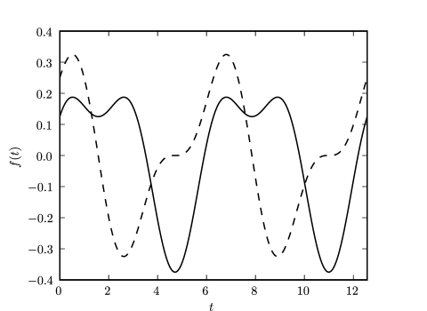
Figure 1: $f(t)=\frac{1}{4}\left[\sin(t)+\frac{1}{2}\cos(2t)\right]$ (solid) and $f(t)=\frac{1}{4}\left[\cos(t)+\frac{1}{2}\sin(2t)\right]$ (dashed line)

As can be seen in Figure 1 there is a qualitative difference in the potentials described by (19) and (20). Especially time-reversal parity ($V(-x,-t)=V(x,t)$) is present in (20) after a time shift of $\pi/(2\omega)$ while it is broken in (19), where time-reversal symmetry ($V(x,-t)=V(x,t)$) is fulfilled after $t\rightarrow t+\pi/(2\omega)$.

IV.1 Asymptotic average current

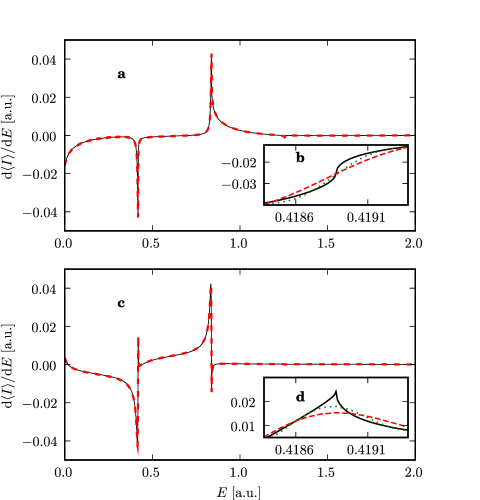
Figure 2: (Color online) ${\rm d}\langle I\rangle/{\rm d}E$ for case I (a, b) and case II (c, d) calculated with Floquet scattering theory (black solid lines) and time-dependent solution (red dashed lines). Parameters are in both cases $d=3$ a.u., $A=2B=0.25$ a.u., $\omega=2\pi/15~{}\mathrm{a.u.}\approx 0.419~{}\mathrm{a.u.}$ Numerical parameters of time evolution are $\Delta x=0.01$ a.u. and $\delta=0.05$ a.u. The time-dependent result is plotted for $t=5000$ a.u. and $x=0$ (the green dotted lines in the insets show the result for $t=10000$ a.u.). The scattering matrix has been computed with $11$ Floquet modes for (a), (c) and $17$ for the insets.

Although cases I and II have different symmetry properties, our numerical results for the integrand of the current, ${\rm d}\langle I\rangle/{\rm d}E$ in (8), in case of a ratio of $A/B=2/1$ are of the same order of magnitude, as can be seen in Figure 2. In the weak-coupling limit it has been found for the tight-binding scheme that the current vanishes in linear order when time-reversal parity is present Lehmann et al. (2003); Kohler et al. (2005). Clearly, there is no weak-coupling limit within the TDSE we solved here and therefore in our case II, by effectively going to arbitrarily high orders, we have found a non-vanishing current. Furthermore, we stress that the results from Floquet scattering theory and the converged time-dependent ones shown in Figure 2 coincide within numerical accuracy.

The characteristic jumps in ${\rm d}\langle I\rangle/{\rm d}E(E)$ at $E=n\omega$ ($n\in\mathbb{N}$) displayed in Figure 2 arise from the fact that at those energies another scattering channel is opening because $E-n\omega$ becomes bigger than zero. In other words, there is another Floquet mode with real wavenumber. The sums in (8) contain one more term, but that is not the only reason for the changes in ${\rm d}\langle I\rangle/{\rm d}E$ because then we would find a step-like change. A characteristic behavior near $E=n\omega$ in the sense of high or discontinuous slopes can already be found for $|S^{m0}_{\alpha\beta}|^{2}$ as a function of $E$ (not shown). The reason is that the matching conditions are sensible to changes in $E$ when the wavenumber for a Floquet mode is near zero and changes from imaginary to real for increasing $E$. In the insets of Figure 2 the convergence characteristics of the time-dependent results near $E=\omega$ are displayed and it is shown that increasing the final time improves the results towards the Floquet result. Nevertheless, at $E\approx\omega$, the convergence is comparative slow.

IV.2 Time-dependent current

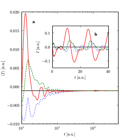
Figure 3: (Color online) Time-dependent results for $\langle I\rangle(x,t)$ (a) and $I(x,t)$ (b) in case I at $x=-d/2$ (blue dotted), $x=0$ (red solid) and $x=d/2$ (green dashed). Parameters are the same as in Figure 2, $E_{F}=0.3$ a.u. and we have discretized the integration in Eq. (17) for 100 values of $k$. For comparison the scattering matrix has been computed with matrices with $11$ Floquet modes and for 2000 energy-values between $0$ and $E_{F}$. Discretized integration according to (8) gives $\langle I\rangle=-1.11\times 10^{-3}$ a.u. (black lines).

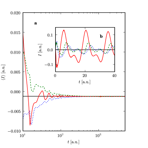
Figure 4: (Color online) Time-dependent results for $\langle I\rangle$ (a) and $I$ (b) in case II at $x=-d/2$ (blue dotted), $x=0$ (red solid) and $x=d/2$ (green dashed). All calculations has been done for the same parameters and in the same way as for Fig. 3. The result of Floquet scattering theory is $\langle I\rangle=-1.21\times 10^{-3}$ a.u. (black lines).

To show the time dependence of the current after switching on the potential in the cases I and II, $\langle I\rangle(x,t)$ is plotted on a logarithmic time scale (Figures 3 and 4, respectively). As in Stefanucci et al. (2008) the results for the middle ($x=0$) as well as for the left and right sides ($x=\pm d/2$) of the central region are shown with different colors (line styles). Although $I(x,t)$ seems to be nearly time-periodic after only one period of time (see insets of Figures 3 and 4), there are changes in $I(x,t)$ for longer times, which can be seen in the behavior of $\langle I\rangle(x,t)$ that needs about $10^{3}$ a.u. to coincide approximately with the result from Floquet scattering theory.

Furthermore, we note that for both potentials, the amplitude of the current (see insets in Figures 3 and 4) is much higher at $x=0$ than at $x=\pm d/2$. This means, in these dipole fields, there exists periodic forward and backward electronic transport which does not arrive at the leads.

IV.3 Optimization of mixing parameter

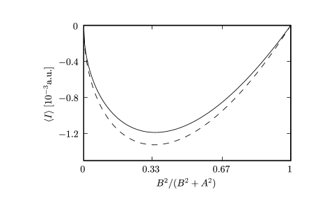
Figure 5: $\langle I\rangle$ as a function of $B^{2}/(B^{2}+A^{2})$ for case I (solid) and case II (dashed). The energy integral in (8) has been discretized by using 100 energy values between 0 and $E_{F}=0.3~{}{\rm a.u.}$ Calculations have been performed again with $11$ Floquet modes.

So far we had used the ratio $A/B=2/1$ for the relative strength of first and second harmonic. In order to find the optimal mixing parameter $B^{2}/(B^{2}+A^{2})$ we have calculated the average current (8) for a fixed Fermi energy of $E_{F}=0.3$ a.u. and for a fixed value of $A^{2}+B^{2}=0.078125$ a.u. using Floquet scattering theory. We refrain from doing time-dependent calculations here as the agreements of the results has been shown above and as the time-dependent calculation is numerically more costly. One finds that to achieve high values of $|\langle I\rangle|$ it is not optimal to use a ratio of $A/B=2/1$ (thus $B^{2}/(A^{2}+B^{2})=0.2$) as done in the numerical examples before. The results presented in Fig. 5 shows a minimum (i.e. a maximum in the absolute value) in the mixing parameter at $0.34$ for both cases.

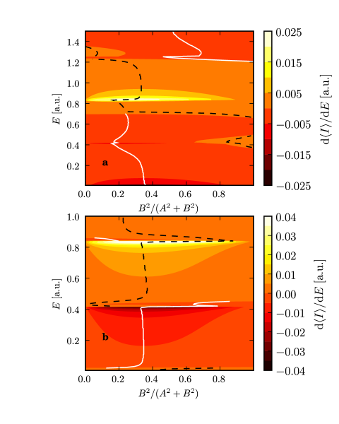
Figure 6: (Color online) Contour plot of ${\rm d}\langle I\rangle/{\rm d}E$ as a function of the incoming energy $E$ and the mixing parameter $B^{2}/(A^{2}+B^{2})$ with fixed $A^{2}+B^{2}=0.078125$ a.u. for case I (a) and II (b). The maximum (black dashed) and the minimum (white solid lines) of ${\rm d}\langle I\rangle/{\rm d}E$ for fixed $E$ are highlighted. We take once more Floquet modes with energy between $E-5\omega$ and $E+5\omega$ into account.

In order to elucidate which energy contributes dominantly to the current, we look at the differential expression ${\rm d}\langle I\rangle/{\rm d}E$ defined in (8) for different values of the incoming energy $E$ and the parameters $A$ and $B$ in (19) and (20) again for a fixed value of $A^{2}+B^{2}=0.078125$ a.u. In the limits of either $B=0$ or $A=0$, ${\rm d}\langle I\rangle/{\rm d}E$ is zero as generalized parity is valid in these cases. In Figure 6 the results of the calculation are shown in a contour plot. The maximum and minimum of ${\rm d}\langle I\rangle/{\rm d}E$ as a function of $B^{2}/(A^{2}+B^{2})$ for fixed $E$ are highlighted. For several values of $E$ an extremum of ${\rm d}\langle I\rangle/{\rm d}E$ as a function of $B^{2}/(A^{2}+B^{2})$ lies around $0.33$ thus $B^{2}/A^{2}\approx 1/2$ especially in case II. On the other hand there are no sharp maxima or minima for variable $B$ in contrast to ${\rm d}\langle I\rangle/{\rm d}E$ as a function of $E$ for a fixed potential. Thus $|\langle I\rangle|$ depends more sensitive on the Fermi energy than on the mixing parameter.

Finally, it is known from classical Hänggi and Marchesoni (2009) as well as from tight-binding calculations Goychuk and Hänggi (1998) that typical harmonic mixing signals for a time-dependent force $F\propto A\cos(\omega t)+B\cos(2\omega t+\phi)$ are in lowest order proportional to $A^{2}B\cos(\phi)$. Our cases I and II correspond to $\phi=\pi$ (I) and $\phi=-\pi/2$ (II), respectively. The proportionality to $A^{2}B$ is equivalent to a proportionality to $\sqrt{x}-\sqrt{x^{3}}$ in the mixing parameter $x:=B^{2}/(B^{2}+A^{2})$ for constant $A^{2}+B^{2}$, which leads to an extremum at $x=1/3$. For the situation considered here, the numerical results show that this dependence on the mixing parameter can be found for a large range of incoming energies (see Fig. 6) and in the integrated current plotted in Fig. 5. The simple dependence on the phase $\phi$, however, is not observed in general.

V Conclusions and Outlook

We have investigated a potential with broken (generalized) parity in order to generate non-zero net currents in unbiased systems. As expected, in the long-time limit, the values from time-dependent calculations using open boundaries agree with the results of the Floquet scattering theory obtained from the matching conditions. The characteristic behavior of ${\rm d}\langle I\rangle/{\rm d}E(E)$ where $E/\omega$ is an integer can be understood as the opening of another Floquet channel for the scattering. Optimization of the mixing parameter $B^{2}/(A^{2}+B^{2})$ shows that for a large range of energies a value close to 0.33 leads to a maximum current amplitude.

In our example the potential is zero in the leads but the applied methodology can also be used for systems with time-dependent potentials in the leads. Floquet scattering theory is numerically less costly than time evolution for the case considered here, but it is restricted to problems where the time dependence is periodic and the analytical solution of the TDSE must be known within certain intervals. Moreover a numerical treatment is only possible if a finite number of Floquet modes have a substantial contribution to the full solutions of the TDSE.

The time-dependent calculation, however, is not restricted to periodic problems and it provides information about the time it takes after switching on a potential to arrive at the quasi-stationary Floquet results. This time may be of interest for microelectronics applications. The algorithm of time evolution can be used for tight-binding problems as well as for the continuous TDSE considered here. For the solution of Kohn-Sham equations within TDDFT the algorithm has been used recently by Kurth et al. Kurth et al. (2010).

Appendix A Floquet S matrix for the harmonic-mixing problem

In this appendix we give details of the Floquet approach to scattering in time-periodic potentials for the harmonic mixing problem studied herein.

To start the discussion, we first briefly review the case of a monochromatic potential of the form $V(x,t)=Ax\cos(\omega t)$. There the so-called Volkov-solution of the TDSE reads Li and Reichl (2000)

$$\psi(x,t)=e^{-if(x,t)}\sum_{n=-\infty}^{\infty}\left[\tilde{a}_{n}e^{iq_{n}g(x,t)}+\tilde{b}_{n}e^{-iq_{n}g(x,t)}\right]e^{-in\omega t},$$ (21)

wherein the definitions

$$f(x,t) = \epsilon t+\int^{t}{\rm d}t^{\prime}~{}V(x,t^{\prime})+h(t)=\epsilon t+\frac{A}{\omega}x\sin(\omega t)-\frac{A^{2}}{8\omega^{3}}\sin(2\omega t),$$ (22)

$$g(x,t) = x+\int^{t}{\rm d}t^{\prime}\int^{t^{\prime}}{\rm d}t^{\prime\prime}~{}V(x,t^{\prime\prime})/x=x-\frac{A}{\omega^{2}}\cos(\omega t),$$ (23)

$$q_{n} = \sqrt{2\left(\epsilon-A^{2}/(4\omega^{2})+n\omega\right)}$$ (24)

have been used.

The Ansatz (21) is now made for the harmonic-mixing potential $V(x,t)=x\left[A\sin(\omega t)+B\cos(2\omega t)\right]$, with the new definitions

$$f(x,t) = \epsilon t+\int^{t}{\rm d}t^{\prime}V(x,t^{\prime})+h(t)=\epsilon t+x\left[-\frac{A}{\omega}\cos(\omega t)+\frac{B}{2\omega}\sin(2\omega t)\right]+h(t),$$ (25)

$$g(x,t) = x+\int^{t}{\rm d}t^{\prime}\int^{t^{\prime}}{\rm d}t^{\prime\prime}\frac{V(x,t^{\prime\prime})}{x}=x-\frac{A}{\omega^{2}}\sin(\omega t)-\frac{B}{4\omega^{2}}\cos(2\omega t)$$ (26)

and $q_{n}=\sqrt{2(\epsilon+C_{0}+n\omega)}$ with constant $C_{0}$. For $h(t)$ after some algebra, we get the following ordinary differential equation,

$$\dot{h}=\frac{A^{2}}{4\omega^{2}}\cos(2\omega t)-\frac{B^{2}}{16\omega^{2}}\cos(4\omega t)-\frac{AB}{4\omega^{2}}\left[\sin(3\omega t)+\sin(\omega t)\right]+\frac{A^{2}}{4\omega^{2}}+\frac{B^{2}}{16\omega^{2}}+C_{0}.$$ (27)

The choice $C_{0}=-A^{2}/(4\omega^{2})-B^{2}/(16\omega^{2})$ warrants that $h(t)$ is periodic so that $\epsilon$ is the Floquet energy. Simple integration leads to

$$h(t)=\frac{A^{2}}{8\omega^{3}}\sin(2\omega t)-\frac{B^{2}}{64\omega^{3}}\sin(4\omega t)+\frac{AB}{12\omega^{3}}\cos(3\omega t)+\frac{AB}{4\omega^{3}}\cos(\omega t),$$ (28)

which completes the solution in the central region $C$ in case I of Sec. IV: Regarding the potential (19) for $t>0$, the analytical solution of the TDSE can be written down in each of the regions $x<-d/2~{}(L)$, $|x|<d/2~{}(C)$ and $x>d/2~{}(R)$,

$$\psi_{L}(x,t) = e^{-i\epsilon t}\sum_{n}\left[\frac{a_{L}^{n}}{\sqrt{k_{n}}}e^{ik_{n}x}+\frac{b_{L}^{n}}{\sqrt{k_{n}}}e^{-ik_{n}x}\right]e^{-in\omega t},$$ (29)

$$\psi_{R}(x,t) = e^{-i\epsilon t}\sum_{n}\left[\frac{a_{R}^{n}}{\sqrt{k_{n}}}e^{-ik_{n}x}+\frac{b_{R}^{n}}{\sqrt{k_{n}}}e^{ik_{n}x}\right]e^{-in\omega t},$$ (30)

$$\psi_{C}(x,t) = e^{-if(x,t)}\sum_{n}\left[\frac{a^{n}}{\sqrt{q_{n}}}e^{iq_{n}g(x,t)}+\frac{b^{n}}{\sqrt{q_{n}}}e^{-iq_{n}g(x,t)}\right]e^{-in\omega t}$$ (31)

with $q_{n}$, $f(x,t)$, $g(x,t)$ as determined before and $k_{n}=\sqrt{2(\epsilon+n\omega)}$. The matching conditions at $x_{L}=-d/2$ and $x_{R}=d/2$ are

$$\psi_{L}\left(x_{L}-0,t\right) = \psi_{C}\left(x_{L}+0,t\right),$$ (32)

$$\psi_{L}^{\prime}\left(x_{L}-0,t\right) = \psi_{C}^{\prime}\left(x_{L}+0,t\right),$$ (33)

$$\psi_{R}\left(x_{R}+0,t\right) = \psi_{C}\left(x_{R}-0,t\right),$$ (34)

$$\psi_{R}^{\prime}\left(x_{R}+0,t\right) = \psi_{C}^{\prime}\left(x_{R}-0,t\right).$$ (35)

Employing the operator $\frac{\omega}{2\pi}\int_{0}^{\frac{2\pi}{\omega}}{\rm d}t~{}e^{is\omega t}$ ($s\in\mathbb{Z}$) on the matching conditions above, i.e., make a Fourier transformation, results in

$$\frac{a_{L}^{s}}{\sqrt{k_{s}}}e^{-ik_{s}d/2}+\frac{b_{L}^{s}}{\sqrt{k_{s}}}e^{ik_{s}d/2}=\sum_{n}\left[\frac{a^{n}}{\sqrt{q_{n}}}e^{-iq_{n}d/2}C^{L+}_{sn}+\frac{b^{n}}{\sqrt{q_{n}}}e^{iq_{n}d/2}C^{L-}_{sn}\right],$$ (36)

$$\begin{split}\sqrt{k_{s}}\left(a_{L}^{s}e^{-ik_{s}d/2}-b_{L}^{s}e^{ik_{s}d/2}\right)=\sum_{n}&\left(a^{n}e^{-iq_{n}d/2}\left[C^{L+}_{sn}\sqrt{q_{n}}+\frac{D^{L+}_{sn}}{\sqrt{q_{n}}}\right]\right.\\ &\left.+b^{n}e^{iq_{n}d/2}\left[-C^{L-}_{sn}\sqrt{q_{n}}+\frac{D^{L-}_{sn}}{\sqrt{q_{n}}}\right]\right),\end{split}$$ (37)

$$\frac{a_{R}^{s}}{\sqrt{k_{s}}}e^{-ik_{s}d/2}+\frac{b_{R}^{s}}{\sqrt{k_{s}}}e^{ik_{s}d/2}=\sum_{n}\left[\frac{a^{n}}{\sqrt{q_{n}}}e^{iq_{n}d/2}C^{R+}_{sn}+\frac{b^{n}}{\sqrt{q_{n}}}e^{-iq_{n}d/2}C^{R-}_{sn}\right],$$ (38)

$$\begin{split}\sqrt{k_{s}}\left(-a_{R}^{s}e^{-ik_{s}d/2}+b_{R}^{s}e^{ik_{s}d/2}\right)=\sum_{n}&\left(a^{n}e^{iq_{n}d/2}\left[C^{R+}_{sn}\sqrt{q_{n}}+\frac{D^{R+}_{sn}}{\sqrt{q_{n}}}\right]\right.\\ &\left.+b^{n}e^{-iq_{n}d/2}\left[-C^{R-}_{sn}\sqrt{q_{n}}+\frac{D^{R-}_{sn}}{\sqrt{q_{n}}}\right]\right).\end{split}$$ (39)

where the definitions

$$C^{\alpha\pm}_{sn} = 1/T\int_{0}^{T}{\rm d}t~{}\exp(i\left[(s-n)\omega t-F\left(x_{\alpha},t\right)\pm q_{n}G(t)\right]),$$ (40)

$$D^{\alpha\pm}_{sn} = -1/T\int_{0}^{T}{\rm d}t~{}F^{\prime}(t)\exp(i\left[(s-n)\omega t-F\left(x_{\alpha},t\right)\pm q_{n}G(t)\right])$$ (41)

have been introduced with $\alpha=L,R$ and $F(x,t)=f(x,t)-\epsilon t$, $G(t)=g(x,t)-x$, $T=2\pi/\omega$. By introducing the diagonal matrices $(E)_{km}=\delta_{km}\exp(iq_{m}d/2)$, $(X)_{km}=\delta_{km}\exp(ik_{m}d/2)$, $(Q)_{km}=\delta_{km}\sqrt{q_{m}}$, $(K)_{km}=\delta_{km}\sqrt{k_{m}}$, it is possible to write the matching conditions in matrix form,

$$K^{-1}X^{-1}a_{L}+K^{-1}Xb_{L} = C^{L+}Q^{-1}E^{-1}a+C^{L-}Q^{-1}Eb,$$ (42)

$$KX^{-1}a_{L}-KXb_{L} = \left[C^{L+}QE^{-1}+D^{L+}Q^{-1}E^{-1}\right]a$$ (43)

$$+\left[-C^{L-}QE+D^{L-}Q^{-1}E\right]b,$$

$$K^{-1}X^{-1}a_{R}-KXb_{R} = C^{R+}Q^{-1}Ea+C^{R-}Q^{-1}E^{-1}b,$$ (44)

$$-KX^{-1}a_{R}+KXb_{R} = \left[C^{R+}QE+D^{R+}Q^{-1}E\right]a$$ (45)

$$+\left[-C^{R-}QE^{-1}+D^{R-}Q^{-1}E^{-1}\right]b.$$

To get an expression for the Floquet scattering matrix $S$ defined in Eq. (7) we need $b_{L}$ and $b_{R}$ in dependence of $a_{L}$ and $a_{R}$. By multiplying Eq. (42) from the left with the matrix $K$ and Eq. (43) with $K^{-1}$ it is possible to eliminate the coefficient $b_{L}$. For $a_{L}$ we find the following expression in dependence of $a$ and $b$,

$$\begin{split}a_{L}=&\underbrace{\frac{X}{2}\left[KC^{L+}Q^{-1}+K^{-1}C^{L+}Q+K^{-1}D^{L+}Q^{-1}\right]E^{-1}}_{=:B_{1}}a\\ &+\underbrace{\frac{X}{2}\left[KC^{L-}Q^{-1}-K^{-1}C^{L-}Q+K^{-1}\right]E}_{=:B_{2}}b.\end{split}$$ (46)

In the same manner we can eliminate $b_{R}$ from Eq. (44) and Eq. (45) and get

$$\begin{split}a_{R}=&\underbrace{\frac{X}{2}\left[KC^{R+}Q^{-1}-K^{-1}C^{R+}Q-K^{-1}D^{R+}Q^{-1}\right]E}_{=:B_{3}}a\\ &+\underbrace{\frac{X}{2}\left[KC^{R-}Q^{-1}+K^{-1}C^{R-}Q-K^{-1}D^{R-}Q^{-1}\right]E^{-1}}_{=:B_{4}}b.\end{split}$$ (47)

Eliminating now the coefficients for the incoming waves $a_{L}$ and $a_{R}$ from Eqs. (42), (43) or (44),(45), respectively, we find

$$\begin{split}b_{L}=&\underbrace{\frac{X^{-1}}{2}\left[KC^{L+}Q^{-1}-K^{-1}C^{L+}Q-K^{-1}D^{L+}Q^{-1}\right]E^{-1}}_{=:B_{5}}a\\ &+\underbrace{\frac{X^{-1}}{2}\left[KC^{L-}Q^{-1}+K^{-1}C^{L-}Q-K^{-1}D^{L-}Q^{-1}\right]E}_{=:B_{6}}b\end{split}$$ (48)

and

$$\begin{split}b_{R}=&\underbrace{\frac{X^{-1}}{2}\left[KC^{R+}Q^{-1}+K^{-1}C^{R+}Q+K^{-1}D^{R+}Q^{-1}\right]E}_{=:B_{7}}a\\ &+\underbrace{\frac{X^{-1}}{2}\left[KC^{R-}Q^{-1}-K^{-1}C^{R-}Q+K^{-1}D^{R-}Q^{-1}\right]E^{-1}}_{=:B_{8}}b.\end{split}$$ (49)

Converting Eq. (46) leads to $a=B_{1}^{-1}\left(a_{L}-B_{2}b\right)$. Putting this in Eq. (47) results in $B_{3}B_{1}^{-1}\left(a_{L}-B_{2}b\right)+B_{4}b=a_{R}$. Converting that to an expression for $b$ yields

$$b=\underbrace{\left[B_{4}-B_{3}B_{1}^{-1}B_{2}\right]^{-1}}_{=:M_{2}^{-1}}\left(a_{R}-B_{3}B_{1}^{-1}a_{L}\right).$$ (50)

One the other hand one gets from Eq. (47) $b=B_{4}^{-1}\left(a_{R}-B_{3}a\right)$. Putting this in Eq. (46) then leads to $\left(B_{1}-B_{2}B_{4}^{-1}B_{3}\right)a+B_{2}B_{4}^{-1}a_{R}=a_{L}$ and thus we find

$$a=\underbrace{\left[B_{1}-B_{2}B_{4}^{-1}B_{3}\right]^{-1}}_{=:M_{1}^{-1}}\left(a_{L}-B_{2}B_{4}^{-1}a_{R}\right).$$ (51)

Putting the equations (50) and (51) in Eqs. (48) and (49) we directly get

$$b_{L}=B_{5}M_{1}^{-1}\left(a_{L}-B_{2}B_{4}^{-1}a_{R}\right)+B_{6}M_{2}^{-1}\left(a_{R}-B_{3}B_{1}^{-1}a_{L}\right),$$ (52)

$$b_{R}=B_{7}M_{1}^{-1}\left(a_{L}-B_{2}B_{4}^{-1}a_{R}\right)+B_{8}M_{2}^{-1}\left(a_{R}-B_{3}B_{1}^{-1}a_{L}\right).$$ (53)

We find

$$S_{LR} = -B_{5}M_{1}^{-1}B_{2}B_{4}^{-1}+B_{6}M_{2}^{-1},$$ (54)

$$S_{RL} = B_{7}M_{1}^{-1}-B_{8}M_{2}^{-1}B_{3}B_{1}^{-1}.$$ (55)

As only $S_{LR}$ and $S_{RL}$ are needed to calculate $\langle I\rangle$ in Eq. (8), we have found expressions for the relevant parts of the Floquet S matrix for the considered system with harmonic mixing.

References

• Switkes et al. (1999) M. Switkes, C. M. Marcus, K. Campman, and A. C. Gossard, Science 283, 1905 (1999).
• DiCarlo and Marcus (2003) L. DiCarlo and C. M. Marcus, J. S. Harris, Jr., Phys. Rev. Lett. 91, 246804 (2003).
• Vavilov et al. (2005) M. G. Vavilov, L. DiCarlo, and C. M. Marcus, Phys. Rev. B 71, 241309 (2005).
• Leek et al. (2005) P. J. Leek, M. R. Buitelaar, V. I. Talyanskii, C. G. Smith, D. Anderson, G. A. C. Jones, J. Wei, and D. H. Cobden, Phys. Rev. Lett. 95, 256802 (2005).
• Linke et al. (1999) H. Linke, T. E. Humphrey, A. Löfgren, A. O. Sushkov, R. Newbury, R. P. Taylor, and P. Omling, Science 286, 2314 (1999).
• Linke et al. (2002) H. Linke, T. E. Humphrey, P. E. Lindelof, A. Löfgren, R. Newbury, P. Omling, A. O. Sushkova, R. P. Taylor, and H. Xu, Applied Physics A: Materials Science & Processing 75, 237 (2002).
• Majer et al. (2003) J. B. Majer, J. Peguiron, M. Grifoni, M. Tusveld, and J. E. Mooij, Phys. Rev. Lett. 90, 056802 (2003).
• Thouless (1983) D. J. Thouless, Phys. Rev. B 27, 6083 (1983).
• Brouwer (1998) P. W. Brouwer, Phys. Rev. B 58, R10135 (1998).
• Zhou et al. (1999) F. Zhou, B. Spivak, and B. Altshuler, Phys. Rev. Lett. 82, 608 (1999).
• Tien and Gordon (1963) P. K. Tien and J. P. Gordon, Phys. Rev. 129, 647 (1963).
• Büttiker and Landauer (1982) M. Büttiker and R. Landauer, Phys. Rev. Lett. 49, 1739 (1982).
• Li and Reichl (1999) W. Li and L. E. Reichl, Phys. Rev. B 60, 15732 (1999).
• Tang and Chu (1999) C. S. Tang and C. S. Chu, Phys. Rev. B 60, 1830 (1999).
• Li and Reichl (2000) W. Li and L. E. Reichl, Phys. Rev. B 62, 8269 (2000).
• Martinez and Reichl (2001) D. F. Martinez and L. E. Reichl, Phys. Rev. B 64, 245315 (2001).
• Zhou and Li (2005) G. Zhou and Y. Li, Journal of Physics: Condensed Matter 17, 6663 (2005).
• Emmanouilidou and Reichl (2002) A. Emmanouilidou and L. E. Reichl, Phys. Rev. A 65, 033405 (2002).
• Kim (2002) S. W. Kim, Phys. Rev. B 66, 235304 (2002).
• Moskalets and Büttiker (2002) M. Moskalets and M. Büttiker, Phys. Rev. B 66, 205320 (2002).
• Camalet et al. (2003) S. Camalet, J. Lehmann, S. Kohler, and P. Hänggi, Phys. Rev. Lett. 90, 210602 (2003).
• Kohler et al. (2005) S. Kohler, J. Lehmann, and P. Hänggi, Physical Reports 406, 379 (2005).
• Lehmann et al. (2003) J. Lehmann, S. Kohler, P. Hänggi, and A. Nitzan, The Journal of Chemical Physics 118, 3283 (2003).
• Goychuk and Hänggi (1998) I. Goychuk and P. Hänggi, EPL (Europhysics Letters) 43, 503 (1998).
• Stafford and Wingreen (1996) C. A. Stafford and N. S. Wingreen, Phys. Rev. Lett. 76, 1916 (1996).
• Arrachea (2005) L. Arrachea, Phys. Rev. B 72, 125349 (2005).
• Arrachea and Moskalets (2006) L. Arrachea and M. Moskalets, Phys. Rev. B 74, 245322 (2006).
• Kurth et al. (2005) S. Kurth, G. Stefanucci, C.-O. Almbladh, A. Rubio, and E. K. U. Gross, Phys. Rev. B 72, 035308 (2005).
• Stefanucci et al. (2008) G. Stefanucci, S. Kurth, A. Rubio, and E. K. U. Gross, Phys. Rev. B 77, 075339 (2008).
• Hänggi and Marchesoni (2009) P. Hänggi, F. Marchesoni, Rev. Mod. Phys. 81, 387 (2009).
• Cini (1980) M. Cini, Phys. Rev. B 22, 5887 (1980).
• Khosravi et al. (2009) E. Khosravi, G. Stefanucci, S. Kurth, and E. K. U. Gross, Physical Chemistry Chemical Physics 11, 4535 (2009).
• Henseler et al. (2001) M. Henseler, T. Dittrich, and K. Richter, Phys. Rev. E. 64, 046218 (2001).
• Hellums and Frensley (1994) J. R. Hellums and W. R. Frensley, Phys. Rev. B 49, 2904 (1994).
• Henseler et al. (2000) M. Henseler, T. Dittrich, and K. Richter, Europhys. Lett. 49, 289 (2000).
• Grossmann (2004) F. Grossmann, Phys. Rev. B 70, 113306 (2004).
• Grossmann et al. (2006) F. Grossmann, M. Fischer, T. Kunert, and R. Schmidt, Chemical Physics 322, 144 (2006).
• Lefebvre and Atabek (2005) R. Lefebvre and O. Atabek, Journal of Physics B: Atomic, Molecular and Optical Physics 38, 2133 (2005).
• Jääskeläinen et al. (2008) M. Jääskeläinen, F. Corvino, C. P. Search, and V. Fessatidis, Phys. Rev. B 77, 155319 (2008).
• Gärttner et al. (2010) M. Gärttner, F. Lenz, C. Petri, F. K. Diakonos, and P. Schmelcher, Phys. Rev. E 81, 051136 (2010).
• Kramer et al. (2010) T. Kramer, C. Kreisbeck, and V. Krueckl, Physica Scripta 82, 038101 (2010).
• Kurth et al. (2010) S. Kurth, G. Stefanucci, E. Khosravi, C. Verdozzi, and E. K. U. Gross, Phys. Rev. Lett. 104, 236801 (2010).