Distributed Detection over Random Networks: Large Deviations Performance Analysis

Abstract

We study the large deviations performance, i.e., the exponential decay rate of the error probability, of distributed detection algorithms over random networks. At each time step $k$ each sensor: 1) averages its decision variable with the neighbors decision variables; and 2) accounts on-the-fly for its new observation. We show that distributed detection exhibits a “phase change” behavior. When the rate of network information flow (the speed of averaging) is above a threshold, then distributed detection is asymptotically equivalent to the optimal centralized detection, i.e., the exponential decay rate of the error probability for distributed detection equals the Chernoff information. When the rate of information flow is below a threshold, distributed detection achieves only a fraction of the Chernoff information rate; we quantify this achievable rate as a function of the network rate of information flow. Simulation examples demonstrate our theoretical findings on the behavior of distributed detection over random networks.

Keywords: Chernoff information, distributed detection, random network, running consensus, information flow, large deviations.

I Introduction

Existing literature on distributed detection can be broadly divided into three different classes. The first studies parallel (fusion) architectures, where all sensors transmit their measurements, or local likelihood ratios, or local decisions, to a fusion node; the fusion node subsequently makes the final decision (see, e.g., [1, 2, 3, 4].) The second considers consensus-based detection, where no fusion node is required, and sensors communicate with single-hop neighbors only over a generic network (see, e.g., [5, 6]). Consensus-based detection operates in two phases. First, in the sensing phase, each sensor collects sufficient observations over a period of time. In the second, communication phase, sensors subsequently run the consensus algorithm to fuse their local log likelihood ratios. More recently, a third class of distributed detection has been proposed (see [7, 8, 9],) where, as with consensus-based detection, sensors communicate over a generic network, and no fusion node is required. Differently than consensus-based detection, sensing and communication phases occur in the same time step. Namely, at each time step $k$, each sensor: 1) exchanges its current decision variable with single-hop neighbors; and 2) processes its new observation, gathered at time step $k$.

In this paper, we focus on the third class of distributed detection, and we provide fundamental analysis of the large deviation performance, i.e., of the exponential decay rate of the error probability (as $k\rightarrow\infty$,) when the underlying communication network is randomly varying. Namely, we show that distributed detection over random networks is asymptotically equivalent to the optimal centralized detection, if the rate of information flow (i.e., the speed of averaging) across the random network is large enough. That is, if the rate of information flow is above a threshold, then the exponential rate of decay of the error probability of distributed detection equals the Chernoff information–the best possible rate of the optimal centralized detector. When the random network has slower information flow (asymptotic optimality cannot be achieved,) we find what fraction of the best possible rate of decay of the error probability distributed detection can achieve; hence, we quantify the tradeoff between the network connectivity and achievable detection performance.

Specifically, we consider the problem where sensors cooperate over a network and sense the environment to decide between two hypothesis. The network is random, varying over time $k$ (see, e.g., [10]); in alternative, the network uses a random communication protocol, like gossip (see, e.g., [11]). The network connectivity is described by $\{W(k)\}_{k=1}^{\infty}$, the sequence of identically distributed (i.i.d.) consensus weight matrices. The sensors’ observations are Gaussian, correlated in space, and uncorrelated in time. At each time $k$, each sensor: 1) communicates with its single-hop neighbors to compute the weighted average of its own and the neighbors’ decision variables; and 2) accounts for its new observation acquired at time $k$. The network’s rate of information flow (i.e., the speed of averaging,) is then measured by $|\log r|$, where $r$ is the second largest eigenvalue of the expected value of $W(k)^{2}$. We then show that distributed detection exhibits a “phase change” behavior. If $|\log r|$ exceeds a threshold, then distributed detection is asymptotically optimal. If $|\log r|$ is below the threshold, then distributed detection achieves only a fraction of the best possible rate; and we evaluate the achievable rate as a function of $r$. Finally, we demonstrate by simulation examples our theoretical findings on the behavior of distributed detection over random networks.

Several recent references [8, 9, 7] consider different variants of distributed detection of the third class. We consider in this paper the running consensus, the variant in [7].

In the context of estimation, distributed iterative schemes have also been proposed. References [12, 13] propose diffusion type LMS and RLS algorithms for distributed estimation; references [14, 15] also propose algorithms for distributed estimation, based on the alternating direction method of multipliers. Finally, reference [16] proposes stochastic-approximation type algorithm for distributed estimation, allowing for randomly varying networks and generic (with finite second moment) observation noise. With respect to the network topology and the observation noise, we also allow for random networks, but we assume Gaussian, spatially correlated observation noise.

We comment on the differences between this work and reference [7], which also studies asymptotic performance of distributed detection via running consensus, with i.i.d. matrices $W(k)$. Reference [7] studies a problem different than ours, in which the means of the sensors’ observations under the two hypothesis become closer and closer; consequently, there is an asymptotic, non zero, probability of miss, and asymptotic, non zero, probability of false alarm. Within this framework, the running consensus achieves the efficacy [17] of the optimal centralized detector, under a mild assumption on the underlying network being connected on average. In contrast, we assume that the means of the distributions do not approach each other as $k$ grows, but stay fixed with $k$. The Bayes error probability exponentially decays to zero, and we examine its rate of decay. We show that, in order to achieve the optimal decay rate of the Bayes error probability, the running consensus needs an assumption stronger than connectedness on average, namely, the averaging speed needs to be sufficiently large (as measured by $|\log r|$.)

In recent work [18], we considered running consensus detection when the underlying network is deterministically time varying; we showed that asymptotic optimality holds if the graph that collects the union of links that are online at least once over a finite time window is connected. In contrast, we consider here the case when the underlying network or the communication protocol are random, and we establish a sufficient condition for optimality in terms of averaging speed (measured by $|\log r|$.)

Paper organization. The next paragraph defines notation that we use throughout the paper. Section II reviews standard asymptotic results in hypothesis testing, in particular, the Chernoff lemma. Section III explains the sensor observations model that we assume and studies the optimal centralized detection, as if there was a fusion node to process all sensors’ observations. Section IV presents the running consensus distributed detection algorithm. Section V studies the asymptotic performance of distributed detection on a simple, yet illustrative, example of random matrices $W(k)$. Section VI studies asymptotic performance of distributed detection in the general case. Section VII demonstrates by simulation examples our theoretical findings. Finally, section VIII concludes the paper.

Notation. We denote by: $A_{ij}$ or $\left[A\right]_{ij}$ (as appropriate) the $(i,j)$-th entry of a matrix $A$; $a_{i}$ or $[a]_{i}$ the $i$-th entry of a vector $a$; $I$, $1$, and $e_{i}$, respectively, the identity matrix, the column vector with unit entries, and the $i$-th column of $I$, $J$ the $N\times N$ matrix $J:=(1/N)11^{\top}$; $\|\cdot\|_{l}$ the vector (respectively, matrix) $l$-norm of its vector (respectively, matrix) argument, $\|\cdot\|=\|\cdot\|_{2}$ the Euclidean (respectively, spectral) norm of its vector (respectively, matrix) argument, $\|\cdot\|_{F}$ the Frobenius norm of a matrix; $\lambda_{i}(\cdot)$ the $i$-th largest eigenvalue, $\mathrm{Diag}\left(a\right)$ the diagonal matrix with the diagonal equal to the vector $a$; $\mathbb{E}\left[\cdot\right]$ and $\mathbb{P}\left(\cdot\right)$ the expected value and probability, respectively; $\mathcal{I}_{\mathcal{A}}$ the indicator function of the event $\mathcal{A}$; finally, $\mathcal{Q}(\cdot)$ the Q-function, i.e., the function that calculates the right tail probability of the standard normal distribution; $\mathcal{Q}(t)=\frac{1}{\sqrt{2\pi}}\int_{t}^{+\infty}e^{-\frac{u^{2}}{2}}du$, $t\in\mathbb{R}$.

II Preliminaries

This section reviews standard asymptotic results in hypothesis testing, in particular, the Chernoff lemma, [19]; it also introduces certain inequalities for the $\mathcal{Q}(\cdot)$ function that we use throughout. We first formally define the binary hypothesis testing problem and the log-likelihood ratio (LLR) test.

Binary hypothesis testing problem: Log-likelihood ratio test. Consider the sequence of independent identically distributed (i.i.d.) $d$-dimensional random vectors (observations) $y(k)$, $k=1,2,...$, and the binary hypothesis testing problem of deciding whether the probability measure generating $y(k)$ is $\nu_{0}$ (under hypothesis $H_{0}$) or $\nu_{1}$ (under $H_{1}$). Assume that $\nu_{1}$ and $\nu_{0}$ are mutually absolutely continuous, distinguishable measures. Based on the observations $y(1),...,y(k)$, formally, a decision test $T$ is a sequence of maps $T_{k}:{\mathbb{R}}^{kd}\rightarrow\{0,1\}$, $k=1,2,...$, with the interpretation that $T_{k}(y(1),...,y(k))=l$ means that $H_{l}$ is decided, $l=0,1$. Specifically, consider the log-likelihood ratio (LLR) test to decide between $H_{0}$ and $H_{1}$, where the $T_{k}$ is given as follows:

$$\mathcal{D}(k) := \frac{1}{k}\sum_{j=1}^{k}L(k)$$ (1)

$$T_{k} = \mathcal{I}_{\{\mathcal{D}(k)>\gamma_{k}\}},$$ (2)

where $L(k):=\log\frac{d\nu_{1}}{d\nu_{0}}\left(y(k)\right)$ is the LLR (given by the Radon-Nikodym derivative of $\nu_{1}$ with respect to $\nu_{0}$ evaluated at $y(k)$,) and $\gamma_{k}$ is a chosen threshold.

Asymptotic Bayes detection performance: Chernoff lemma. Given a test $T$, we are interested in quantifying the detection performance, namely, in determining the Bayes error probability after $k$ data (observation) samples are processed:

$$P^{e}(k)=P\left(H_{0}\right)\alpha(k)+P\left(H_{1}\right)\beta(k),$$ (3)

where $P\left(H_{l}\right)$ are the prior probabilities, $\alpha(k)=\mathbb{P}\left(T_{k}=1|H_{0}\right)$ and $\beta(k)=\mathbb{P}\left(T_{k}=0|H_{1}\right)$ are, respectively, the probability of false alarm and the probability of a miss. Generally, exact evaluation of $\alpha(k)$ and $\beta(k)$ (and hence, $P^{e}(k)$) is very hard (as in the case of distributed detection over random networks that we study; see also [20] for distributed detection on a parallel architecture.) We seek computationally tractable estimates of $P^{e}(k)$, when $k$ grows large. Typically, for large $k$, $P^{e}(k)$ is a small number (i.e., the detection error occurs rarely,) and, in many models, it exponentially decays to zero as $k\rightarrow+\infty$. Thus, it is of interest to determine the (large deviations) rate of exponential decay of $P^{e}(k)$, given by:

$$\lim_{k\rightarrow\infty}\,-\frac{1}{k}\log P^{e}(k).$$ (4)

Lemma 1 ([19, 21]) states that, among all possible decision tests, the LLR test with zero threshold maximizes (4) (i.e., has the fastest decay rate of $P^{e}(k)$.) The corresponding decay rate equals the Chernoff information ${\bf{C}}$, i.e., the Chernoff distance between the distributions of $y(k)$ under $H_{0}$ and $H_{1}$, where ${\bf{C}}$ is given by, [19]:

$${\bf{C}}=\max_{s\in[0,1]}\left\{-\log\int\left(\frac{d\nu_{0}}{d\nu_{1}}\right)^{1-s}d\nu_{1}\right\}.$$ (5)

Lemma 1 (Chernoff lemma)

If $P(H_{0})\in(0,1)$, then:

$$\sup_{T}\left\{\limsup_{k\rightarrow\infty}\,-\frac{1}{k}\log P^{e}(k)\right\}={\bf{C}},$$ (6)

where the supremum over all possible tests $T$ is attained for the LLR test with $\gamma_{k}=0$, $\forall k$.

Asymptotically optimal test. We introduce the following definition of the asymptotically optimal test.

Definition 2

The decision test $T$ is asymptotically optimal if it attains the supremum in eqn. (6).

We will find a necessary condition and a sufficient condition for asymptotic optimality (in the sense of Definition 2) of the running consensus distributed detection.

Inequalities for the standard normal distribution. We will use the following property of the $\mathcal{Q}(\cdot)$ function, namely, that for any $t>0$ (e.g., [22]):

$$\frac{t}{1+t^{2}}e^{-\frac{t^{2}}{2}}\leq\sqrt{2\pi}\,\mathcal{Q}(t)\leq\frac{1}{t}e^{-\frac{t^{2}}{2}}.$$ (7)

III Centralized detection

We proceed with the Gaussian model for which we find (in section V) conditions for asymptotic optimality of the running consensus distributed detection. Subsection III-A describes the model of the sensor observations that we assume. Subsection III-B describes the (asymptotically) optimal centralized detection, as if there was a fusion node that collects and processes the observations from all sensors.

III-A Sensor observations model

We assume that $N$ sensors are deployed to sense the environment and to decide between the two possible hypothesis, $H_{1}$ and $H_{0}$. Each sensor $i$ measures a scalar quantity $y_{i}(k)$ at each time step $k$; all sensors measure at time steps $k=1,2,...$ Collect $y_{i}(k)$’s, $i=1,...,N$, into $N\times 1$ vector $y(k)=(y_{1}(k),...,y_{N}(k))^{\top}$. We assume that $\{y(k)\}$ has the following distribution:

$$\mathrm{Under\,\,}H_{l}:\,y(k)=m_{l}+\zeta(k),\,\,l=0,1.$$ (8)

The quantity $m_{l}$ is the constant signal; the quantity $\zeta(k)$ is zero-mean, Gaussian, spatially correlated noise, i.i.d. across time, with distribution $\zeta(k)\sim\mathcal{N}\left(0,S\right)$, where $S$ is a positive definite covariance matrix. Spatial correlation of the measurements (i.e., non-diagonal covariance matrix $S$) accounts for, e.g., dense deployment in sensor networks.

III-B (Asymptotically) optimal centralized detection

This subsection studies optimal centralized detection under the Gaussian assumptions in III-A, as if there was a fusion node that collects and processes all sensors’ observations. The LLR decision test is given by eqns. (1) and (2), where it is straightforward to show that now the LLR takes the following form:

$$L(k)=(m_{1}-m_{0})^{\top}S^{-1}\left(y(k)-\frac{m_{1}+m_{0}}{2}\right)$$ (9)

Conditioned on either hypothesis $H_{1}$ and $H_{0}$, $L(k)\sim\mathcal{N}\left(m_{L}^{(l)},\sigma_{L}^{2}\right)$, where

$$m_{L}^{(1)} = -m_{L}^{(0)}=\frac{1}{2}(m_{1}-m_{0})^{\top}S^{-1}(m_{1}-m_{0})$$ (10)

$$\sigma_{L}^{2} = (m_{1}-m_{0})^{\top}S^{-1}(m_{1}-m_{0}).$$ (11)

Define the vector $v\in{\mathbb{R}}^{N}$ as

$$v:=S^{-1}(m_{1}-m_{0}).$$ (12)

Then, the LLR $L(k)$ can be written as follows:

$$L(k)=\sum_{i=1}^{N}v_{i}\left(y_{i}(k)-\frac{[m_{1}]_{i}+[m_{0}]_{i}}{2}\right)=\sum_{i=1}^{N}\eta_{i}(k)$$ (13)

Thus, the LLR at time $k$ is separable, i.e., the LLR is the sum of the terms $\eta_{i}(k)$ that depend affinely on the individual observations $y_{i}(k)$. We will exploit this fact in section IV to derive the distributed, running consensus, detection algorithm.

Bayes probability of error: finite number of observations. The minimal Bayes error probability, $P^{e}_{\mathrm{cen}}(k)$, when $k$ samples are processed, and $P(H_{0})=P(H_{1})=\frac{1}{2}$ (equal prior probabilities), is attained for the (centralized) LLR test with zero threshold; $P^{e}_{\mathrm{cen}}(k)$ equals:

$$P^{e}_{\mathrm{cen}}(k)=\mathcal{Q}\left(\sqrt{k}\frac{m_{L}^{(1)}}{\sigma_{L}}\right).$$ (14)

The quantity $P^{e}_{\mathrm{cen}}(k)$ will be of interest when we compare (by simulation, in Section VII) the running consensus detection with the optimal centralized detection, in the regime of finite $k$.

Bayes probability of error: time asymptotic results. The Chernoff lemma (Lemma 1) applies also to the (centralized) detection problem as defined in subsection III-A. It can be shown that the Chernoff information, in this case, equals:

$${\bf{C}}={\bf{C}_{\mathrm{tot}}}=\frac{1}{8}(m_{1}-m_{0})^{\top}S^{-1}(m_{1}-m_{0}).$$ (15)

In eqn. (15), the subscript $\mathrm{tot}$ designates the total Chernoff information of the network, i.e., the Chernoff information of the observations collected from all sensors. Specifically, if the sensor observations are uncorrelated (the noise covariance matrix $S=\mathrm{Diag}(\sigma_{1}^{2},...,\sigma_{N}^{2})$,) then:

$${\bf{C}_{\mathrm{tot}}}=\sum_{i=1}^{N}\frac{[m_{1}-m_{0}]_{i}^{2}}{8\sigma_{i}^{2}}=\sum_{i=1}^{N}{\bf{C}_{i}},$$ (16)

where ${\bf{C}}_{i}$ is the Chernoff information of the individual sensor $i$. That is, ${\bf{C}}_{i}$ equals the best achievable rate of the Bayes error probability, if the sensor $i$ worked as an individual (it did not cooperate with the other sensors.)

Lemma 3

(Chernoff lemma for asymptotically optimal centralized detector) Consider the observation model defined in subsection III-A, and let $P(H_{0})\in(0,1)$. The LLR test with $\gamma_{k}=0$, $\forall k$, is asymptotically optimal in the sense of Definition 2. Moreover, for the LLR test with $\gamma_{k}=0$, $\forall k$, we have:

$$\lim_{k\rightarrow\infty}\frac{1}{k}\log P^{e}_{\mathrm{cen}}(k)=-{\bf{C}_{\mathrm{tot}}},$$ (17)

where ${\bf{C}_{\mathrm{tot}}}$ is given by eqn. (15).

IV Distributed detection

We now consider distributed detection, under the same assumptions on the sensor observations as in III-A; but the fusion node is no longer available, and the sensors cooperate through a randomly varying network. Specifically, we consider the running consensus distributed detection, proposed in [7], and we extend it to spatially correlated observations. At each time $k$, each sensor $i$ improves its decision variable, call it $x_{i}(k)$, two-fold: 1) by exchanging the decision variable locally with its neighbors and computing the weighted average of its own and the neighbors’ variables; and 2) by incorporating its new observation at time $k$.

Recall the definition of the vector $v$ in eqn. (12) and the scalar $\eta_{i}(k)$ in eqn. (13). The update of $x_{i}(k)$ is then as follows:

$$x_{i}(k+1) = \frac{k}{k+1}\left(W_{ii}(k)x_{i}(k)+\sum_{j\in O_{i}(k)}W_{ij}(k)x_{j}(k)\right)+\frac{1}{k+1}\eta_{i}(k+1),\,k=1,...$$ (18)

$$x_{i}(1) = \eta_{i}(1).$$

Here $O_{i}(k)$ is the (random) neighborhood of sensor $i$ at time $k$, and $W_{ij}(k)$ are the (random) averaging weights. The local sensor $i$’s decision test at time $k$, $T_{k,i}$, is given by:

$$T_{k,i}:=\mathcal{I}_{\{x_{i}(k)>0\}},$$ (19)

i.e., $H_{1}$ (resp. $H_{0}$) is decided when $x_{i}(k)>0$ (resp. $x_{i}(k)\leq 0$.) Let $x(k)=(x_{1}(k),x_{2}(k),...,x_{N}(k))^{\top}$ and $\eta(k)=(\eta_{1}(k),...,\eta_{N}(k))^{\top}$. Also, collect the averaging weights $W_{ij}(k)$ in $N\times N$ matrix $W(k)$, where, clearly, $W_{ij}(k)=0$ if the sensors $i$ and $j$ do not communicate at time step $k$. The algorithm in matrix form becomes:

$$x(k+1) = \frac{k}{k+1}W(k)x(k)+\frac{1}{k+1}\eta(k+1),\,k=1,...$$ (20)

$$x(1) = \eta(1).$$

We remark that the algorithm in (20) extends the running consensus algorithm in [23] for spatially correlated sensor observations (non-diagonal covariance matrix $S$.) When $S$ is diagonal, the algorithm in (20) reduces to the algorithm in [23].

We allow the averaging matrices $W(k)$ to be random. Formally, let $(\Omega,\mathcal{F},\mathbb{P})$ be a probability space (where $\Omega$ is a sample space, $\mathcal{F}$ is a $\sigma$-algebra, and $\mathbb{P}:\mathcal{F}\rightarrow[0,1]$ is a probability measure.) For any $k$, $W(k)$ is a random variable, i.e., an $\mathcal{F}$-measurable function $W(k)=W(\omega;k)$, $\omega\in\Omega$, $W(k):\Omega\rightarrow{\mathbb{R}}^{N\times N}$. We now summarize the assumptions on $W(k)$. Recall that $J:=\frac{1}{N}(11^{\top})$ and denote by $\widetilde{W}(k):=W(k)-J$. From now on, we will drop the index $k$ from $W(k)$ and $\widetilde{W}(k)$ when we refer to the distribution of $W(k)$ and $\widetilde{W}(k)$.

Assumption 4

For the sequence of matrices $\left\{W(k)\right\}_{k=1}^{\infty}$, we assume the following:

1. The sequence $\left\{W(k)\right\}_{k=1}^{\infty}$ is i.i.d.

2. $W$ is symmetric and stochastic (row-sums are equal to 1 and the entries are nonnegative,) with probability one.

3. The random matrix $W(l)$ and the random vector $y(s)$ are independent, $\forall l$, $\forall s$.

In sections V and VI, we examine what (additional) conditions the matrices $W(k)$ have to satisfy, to achieve asymptotic optimality of the distributed detection algorithm.

Network supergraph. Define also the network supergraph as a pair $G:=(\mathcal{V},E)$, where $\mathcal{V}$ is the set of nodes with cardinality $|\mathcal{V}|=N$, and $E$ is the set of edges with cardinality $|E|=M$, defined by: $E=\{\{i,j\}:\,\,\mathbb{P}\left(W_{ij}\neq 0\right)>0,\,\,i<j\}.$ Clearly, when, for some $\{i,j\}$, $\mathbb{P}\left(W_{ij}\neq 0\right)=0$, then the link $\{i,j\}\notin E$ and nodes $i$ and $j$ never communicate.

For subsequent analysis, it will be useful to define the matrices $\Phi(k,j)$, for $k>j\geq 1$, as follows:

$$\Phi(k,j):=W(k-1)W(k-2)...W(j).$$ (21)

Then, the algorithm in eqn. (20) can be written as:

$$x(k)=\frac{1}{k}\sum_{j=1}^{k-1}\Phi(k,j)\eta(j)+\frac{1}{k}\eta(k),\,\,k=2,3,...$$ (22)

Also, introduce:

$$\widetilde{\Phi}(k,j):=\widetilde{W}(k-1)\widetilde{W}(k-2)...\widetilde{W}(j),\,\,k>j\geq 1,$$ (23)

and remark that

$$\widetilde{\Phi}(k,j)=\Phi(k,j)-J.$$

Recall the definition of the $N\times 1$ vector $v$ in (12). The sequence of $N\times 1$ random vectors $\{\eta(k)\}$, conditioned on $H_{l}$, is i.i.d. The vector $\eta(k)$ (under hypothesis $H_{l}$, $l=0,1$) is Gaussian with mean $m_{\eta}^{(l)}$ and covariance $S^{\eta}$:

$$m_{\eta}^{(l)} = (-1)^{(l+1)}\mathrm{Diag}\left(v\right)\,\frac{1}{2}(m_{1}-m_{0})$$ (24)

$$S^{\eta} = \mathrm{Diag}\left(v\right)S\mathrm{Diag}\left(v\right).$$ (25)

Here $\mathrm{Diag}(v)$ is a diagonal matrix with the diagonal entries equal to the entries of $v$.

V Asymptotic performance of distributed detection: Switching fusion example

In this section, we examine asymptotic performance of distributed detection algorithm on a simple and impractical, yet illustrative example; we tackle the generic case in Section VI. The network at a time step $k$ can either be fully connected, with probability $p$, or completely disconnected (without edges,) with probability $1-p$. Specifically, the distribution of the random averaging matrix $W(k)$ is given by:

$$W(k)=\left\{\begin{array}[]{ll}J&\mbox{ with prob. $p$}\\ I&\mbox{ with prob. $1-p$.}\end{array}\right.$$ (26)

With model (26), at each time step $k$, each sensor behaves as a fusion node, with probability $p$, and as an individual detector, with probability $1-p$. We call this communication model the switching fusion. We show that, to achieve asymptotic optimality of distributed detection, the fusion step ($W(k)=J$) should occur sufficiently often, i.e., $p$ should exceed a threshold. Namely, we find necessary and sufficient condition for the asymptotic optimality in terms of $p$. When distributed detection is not optimal ($p$ is below the threshold,) we find the achievable rate of decay of the error probability, as a function of $p$. The goal of the switching fusion example is two-fold. First, it provides insight on how the amount of communication (measured by $p$) affects detection performance. Second, it explains in a clear and natural way our methodology for quantifying detection performance on generic networks (in Section VI.) Namely, Section VI mimics and extends the analysis from Section V to derive distributed detection performance on generic networks. We next detail the sensor observations model.

We assume that the observations $y_{i}(k)$ of $N$ different sensors are uncorrelated, and that the individual Chernoff information, given by eqn. (16), is the same at each sensor $i$. Hence, we have ${\bf{C}_{\mathrm{tot}}}=N\,\bf{C_{i}}$. We assume that, at time instant $k$, the network can either be fully connected, with probability $p$, or without edges, with probability $1-p$.

Denote by $P^{e}_{i,\mathrm{dis}}(k)$ the Bayes error probability at sensor $i$, after $k$ samples are processed. We have the following Theorem on the asymptotic performance of the distributed detection algorithm.

Theorem 5

Consider the distributed detection algorithm given by eqns. (18) and (19). Assume that the sensor observations are spatially uncorrelated and that the Chernoff information ${\bf{C_{i}}}$ is equal at each sensor $i$. Let $W(k)$ be i.i.d. matrices with the distribution given by eqn. (26). Then, the exponential decay rate of the error probability is given by:

$$\lim_{k\rightarrow\infty}\,-\frac{1}{k}\log P^{e}_{i,\mathrm{dis}}(k)=\left\{\begin{array}[]{ll}{\bf{C_{\mathrm{tot}}}}&\mbox{ if $|\log(1-p)|\geq{\bf{C_{\mathrm{tot}}}}(N-1)$}\\ {{\bf{C_{i}}}}+|\log(1-p)|&\mbox{ if $|\log(1-p)|\leq\frac{{\bf{C_{\mathrm{tot}}}}(N-1)}{N^{2}}$}\\ 2\sqrt{\frac{|\log(1-p)|{\bf{C_{\mathrm{tot}}}}}{N-1}}-\frac{|\log(1-p)|}{N-1}&\mbox{ otherwise.}\end{array}\right.$$ (30)

Moreover, a necessary and sufficient condition for asymptotic optimality, in the sense of Definition 2, is given by:

$$\frac{|\log(1-p)|}{N-1}\geq{\bf{C_{\mathrm{tot}}}}=N{\bf{C_{i}}}.$$ (31)

Condition (31) says that the network connectivity should be good enough (i.e., $p$ should be large enough,) in order to achieve the asymptotic optimality of distributed detection. Also, there is a “phase change” behavior, in a sense that distributed detection is asymptotically optimal above a threshold on $p$, and it is not optimal below that threshold. Further, we can see that, as $p$ decreases, distributed detection performance becomes worse and worse, and it approaches the performance of an individual sensor-detector. (See Figure 1, and eqn. (30).)

We proceed with proving Theorem 5. In Section VI, we will follow a reasoning similar to the proof of Theorem 5 to provide a sufficient condition for asymptotic optimality on generic networks.

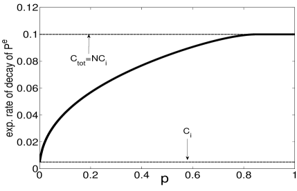
Figure 1: Exponential decay rate of error probability $\phi^{\star}$ (given by eqn. (26)) for the model considered in Section V. The network has $N=20$ sensors and ${\bf{C_{\mathrm{tot}}}}=0.1$. The optimal rate (equal to ${\bf{C_{\mathrm{tot}}}}$) is achieved for $p\geq 0.83$.

Proof of Theorem 5.

First, remark that $x(k)$, conditioned on $H_{0}$, is equal in distribution to $-x(k)$, conditioned on $H_{1}$. This is true because $\eta(k)$, conditioned on $H_{0}$, is equal in distribution to $-\eta(k)$, conditioned on $H_{1}$, for all $k$; and the distribution of $W(k)$ does not depend on the active hypothesis, $H_{0}$ or $H_{1}$. Denote by $\mathbb{P}_{l}\left(\cdot\right)=\mathbb{P}(\cdot|H_{l})$, $l=0,1$, and consider the probability of false alarm, the probability of miss, and the Bayes error probability at sensor $i$ (with the running consensus detector,) respectively, given by:

$$\alpha_{i,\mathrm{dis}}(k) = \mathbb{P}_{0}\left(x_{i}(k)>0\right),\,\,\beta_{i,\mathrm{dis}}(k)=\mathbb{P}_{1}\left(x_{i}(k)\leq 0\right)$$ (32)

$$P^{e}_{i,\mathrm{dis}}(k) = P(H_{0})\mathbb{P}_{0}\left(x_{i}(k)>0\right)+P(H_{1})\mathbb{P}_{1}\left(x_{i}(k)\leq 0\right).$$ (33)

Remark that $\mathbb{P}_{l}\left(x_{i}(k)=0\right)=0$, $l=0,1$. Thus, we have that

$$\beta_{i,\mathrm{dis}}(k) = \mathbb{P}_{1}\left(x_{i}(k)\leq 0\right)=\mathbb{P}_{0}\left(x_{i}(k)>0\right)=\alpha_{i,\mathrm{dis}}(k),\,\,\forall k,\,\,\forall i.$$ (34)

From eqns. (33) and (34), it can be shown that:

$$\limsup_{k\rightarrow\infty}\frac{1}{k}\log P^{e}_{i,\mathrm{dis}}(k) = \limsup_{k\rightarrow\infty}\frac{1}{k}\log\alpha_{i,\mathrm{dis}}(k)$$ (35)

$$\liminf_{k\rightarrow\infty}\frac{1}{k}\log P^{e}_{i,\mathrm{dis}}(k) = \liminf_{k\rightarrow\infty}\frac{1}{k}\log\alpha_{i,\mathrm{dis}}(k).$$ (36)

We further assume that $H_{0}$ is true, and we restrict our attention to $\alpha_{i,\mathrm{dis}}(k)$, but the same conclusions (from (34)) will be valid for $\beta_{i,\mathrm{dis}}(k)$ also. We now make the key step in proving Theorem 5, by defining a partition of the probability space $\Omega$. Fix the time step $k$ and denote by $A_{l}$, $l=0,...,k-1$, the event

$$A_{l}=\left\{\begin{array}[]{ll}\left\{\max\left\{{s\in\{1,...,k-1\}}:\,\,W(s)=J\right\}=l\right\}&\mbox{ for $l=1,...,k-1$}\\ \{W(s)=I,\,s=1,...,k-1\}&\mbox{ for $l=0.$}\end{array}\right.$$

That is, $A_{l}$ is the event that the largest time step $s\leq k-1$, for which $W(s)=J$, is equal to $s=l$. (The event $A_{l}$ includes the scenarios of arbitrary realizations of $W(s)$–either $J$ or $I$–for $s\leq l$; but it requires $W(s)=I$ for all $l<s\leq k-1$.) Remark that $A_{l}$ is a function of $k$, but the dependence on $k$ is dropped for notation simplicity. We have that $\mathbb{P}\left(A_{l}\right)=p(1-p)^{k-l-1}$, for $l=1,...,k-1$, and $\mathbb{P}\left(A_{0}\right)=(1-p)^{k-1}$. Also, each two events, $A_{l}$ and $A_{j}$, $j\neq l$, are disjoint, and $\cup_{l=0}^{k-1}\,A_{l}=\Omega,$ i.e., the events $A_{l}$, $l=0,...,k-1$, constitute a finite partition of the probability space $\Omega$. (Note that $\sum_{l=0}^{k-1}\mathbb{P}(A_{l})=1$.) Recall the definition of $\Phi(k,j)$ in eqn. (21) and note that, if $A_{l}$ occurred, we have:

$$\Phi(k,s)=\left\{\begin{array}[]{ll}I&\mbox{ if $k-1\geq s>l$}\\ J&\mbox{ if $s\leq l$.}\end{array}\right.$$ (37)

Further, conditioned on $A_{l}$, we have that (when $l=0$, first sum in eqn. (V) does not exist)

$$x(k) = \frac{1}{k}\left(\sum_{j=1}^{l}J\eta(j)+\sum_{j=l+1}^{k}I\eta(j)\right)$$

$$= \frac{1}{k}\left(\sum_{j=1}^{l}\left(\frac{1^{\top}\eta(j)}{N}\right)1+\sum_{j=l+1}^{k}\eta(j)\right).$$

Hence, conditioned on $A_{l}$, $x_{i}(k)$ is a Gaussian random variable,

$$x_{i}(k)|A_{l}\sim\mathcal{N}\left(\theta(l;k),\,\zeta^{2}(l;k)\right),$$

where

$$\theta(l;k) = -\frac{4l}{N}{\bf{C_{\mathrm{tot}}}}-4(k-l){\bf{C_{i}}}=-4k{\bf{C_{i}}}$$ (39)

$$\zeta^{2}(l;k) = \frac{8l}{N^{2}}{\bf{C_{\mathrm{tot}}}}+8(k-l){\bf{C_{i}}}.$$ (40)

Define

$$\chi(l;k):=-\frac{\theta(l;k)}{\zeta(l;k)}=\frac{\sqrt{2{\bf{C_{i}}}}{k}}{\sqrt{\frac{l}{N}+(k-l)}},$$ (41)

and remark that

$$\mathbb{P}_{0}\left(x_{i}(k)>0|A_{l}\right)=\mathcal{Q}(\chi(l;k)),$$

where $\mathbb{P}_{0}(\cdot):=\mathbb{P}(\cdot|H_{0})$.

Using the total probability, we can write $\alpha_{i,\mathrm{dis}}(k)=\mathbb{P}_{0}\left(x_{i}(k)>0\right)$ as:

$$\alpha_{i,\mathrm{dis}}(k) = \sum_{l=0}^{k-1}\mathbb{P}_{0}\left(x_{i}(k)>0|A_{l}\right)\,\mathbb{P}(A_{l})$$

$$= \sum_{l=1}^{k-1}\mathcal{Q}(\chi(l;k))\,p(1-p)^{k-l-1}+\mathcal{Q}(\chi(0;k))\,(1-p)^{k-1}.$$

We now proceed with calculating the exponential rate of decay of $\alpha_{i,\mathrm{dis}}(k)$ (and hence, $P^{e}_{i,\mathrm{dis}}(k)$) as $k\rightarrow\infty$. The key ingredient to do that is the representation of $\alpha_{i,\mathrm{dis}}(k)$ in eqn. (V), and the inequalities for the $\mathcal{Q}$-function in eqn. (7). Namely, it can be shown that, when $k$ grows large, $\alpha_{i,\mathrm{dis}}(k)$, and hence, $P^{e}_{i,\mathrm{dis}}(k)$, behaves as (here we present the main idea but precise statements are in the Apendix):

$$P^{e}_{i,\mathrm{dis}}(k)\sim\sum_{j=0}^{k-1}e^{-k\,\phi(j;k)},$$ (43)

where

$$\phi(j;k):=\frac{{\bf{C_{\mathrm{tot}}}}}{1+(N-1)\frac{j+1}{k}}+\frac{j}{k}|\log(1-p)|.$$ (44)

Hence, the quantities $\phi(j;k)$, for different $j$’s, represent different “modes” of decay; the decay of $P^{e}_{i,\mathrm{dis}}(k)$ is then determined by the slowest mode $\widehat{\phi}(k)$, defined by:

$$\widehat{\phi}(k)=\min_{j=0,...,k-1}\phi(j;k).$$ (45)

More precisely, using eqns. (35), (36), the expression for $\alpha_{i,\mathrm{dis}}(k)$ in eqn. (V), and the inequalities (7), it can be shown that:

$$\liminf_{k\rightarrow\infty}\,-\frac{1}{k}\log P^{e}_{i,\mathrm{dis}}(k) \geq \liminf_{k\rightarrow\infty}\widehat{\phi}(k)$$ (46)

$$\limsup_{k\rightarrow\infty}\,-\frac{1}{k}\log P^{e}_{i,\mathrm{dis}}(k) \leq \limsup_{k\rightarrow\infty}\widehat{\phi}(k).$$

The detailed proof of inequalities (46) is in the Appendix.

We proceed by noting that the minimum of $\phi(j;k)$ over the discrete set $j\in\{0,1,...,k-1\}$ does not differ much from the minimum of $\phi(j;k)$ over the interval $[0,k-1]$. Denote by $\phi^{\star}(k)$ the minimum of $\phi(j;k)$ over $[0,k-1]$:

$$\phi^{\star}(k) = \min_{j\in[0,k-1]}\phi(j;k).$$ (47)

Then, it is easy to verify that:

$$\phi^{\star}(k)\leq\widehat{\phi}(k)\leq\phi^{\star}(k)\,(1+\frac{N-1}{k})+\frac{|\log(1-p)|}{k}.$$ (48)

The function $\phi(j,k)$ is convex in its first argument on $j\in[0,k-1]$; it is straightforward to calculate $\phi^{\star}(k)$, which can be shown to be equal to:

$$\phi^{\star}(k)=\left\{\begin{array}[]{ll}\frac{{\bf{C_{\mathrm{tot}}}}}{1+\frac{N-1}{k}}&\mbox{ if $|\log(1-p)|\geq\frac{{\bf{C_{\mathrm{tot}}}}(N-1)}{(1+\frac{N-1}{k})^{2}}$}\\ \frac{{\bf{C_{\mathrm{tot}}}}}{N}+\frac{k-1}{k}|\log(1-p)|&\mbox{ if $|\log(1-p)|\leq\frac{{\bf{C_{\mathrm{tot}}}}(N-1)}{N^{2}}$}\\ 2\sqrt{\frac{|\log(1-p)|{\bf{C_{\mathrm{tot}}}}}{N-1}}-\frac{|\log(1-p)|}{N-1}-\frac{|\log(1-p)|}{k}&\mbox{ otherwise.}\end{array}\right.$$ (52)

The limit $\lim_{k\rightarrow\infty}\phi^{\star}(k)=:\phi^{\star}$ exists, and is equal to:

$$\phi^{\star}=\left\{\begin{array}[]{ll}{\bf{C_{\mathrm{tot}}}}&\mbox{ if $|\log(1-p)|\geq{\bf{C_{\mathrm{tot}}}}(N-1)$}\\ \frac{{\bf{C_{\mathrm{tot}}}}}{N}+|\log(1-p)|&\mbox{ if $|\log(1-p)|\leq\frac{{\bf{C_{\mathrm{tot}}}}(N-1)}{N^{2}}$}\\ 2\sqrt{\frac{|\log(1-p)|{\bf{C_{\mathrm{tot}}}}}{N-1}}-\frac{|\log(1-p)|}{N-1}&\mbox{ otherwise.}\end{array}\right.$$ (56)

From eqns. (48) and (56), we have:

$$\lim_{k\rightarrow\infty}\widehat{\phi}(k)=\lim_{k\rightarrow\infty}\phi^{\star}(k)=\phi^{\star}.$$ (57)

In view of eqns. (57) and (46), it follows that the rate of decay of the error probability at sensor $i$ is:

$$\lim_{k\rightarrow\infty}\,-\frac{1}{k}\log P^{e}_{i,\mathrm{dis}}(k)=\lim_{k\rightarrow\infty}\widehat{\phi}(k)=\phi^{\star}.$$ (58)

The necessary and sufficient condition for asymptotic optimality then follows from eqn. (56).

∎

VI Asymptotic performance of distributed detection: General case

This section provides a necessary condition, and a sufficient condition for asymptotic optimality of distributed detection on generic networks and for generic, spatially correlated, Gaussian observations. When distributed detection is not guaranteed to be optimal, this section finds a lower bound on the exponential decay rate of error probability, in terms of the system parameters. We start by pursuing sufficient conditions for optimality and evaluating the lower bound on the decay rate of the error probability.

VI-A Sufficient condition for asymptotic optimality

Recall that $r:=\lambda_{2}\left(\mathbb{E}\left[W(k)^{2}\right]\right)=\|\mathbb{E}\left[W(k)^{2}\right]-J\|$. It is well known that the quantity $r$ measures the speed of the information flow, i.e., the speed of the averaging across the network, like with standard consensus and gossip algorithms, e.g., [11]. (The smaller $r$ is, the faster the averaging is.) The next Theorem shows that distributed detection is asymptotically optimal if the network information flow is fast enough, i.e., if $r$ is small enough. The Theorem also finds a lower bound on the rate of decay of the error probability, even when the sufficient condition for asymptotic optimality does not hold. Recall also ${\bf{C_{\mathrm{tot}}}}$ in eqn. (16).

Theorem 6

Let Assumption 4 hold and consider the distributed detection algorithm defined by eqns. (18) and (19). Then, the following holds for the exponential decay rate of the error probability at each sensor:

$$\liminf_{k\rightarrow\infty}\,-\frac{1}{k}\log P^{e}_{i,\mathrm{dis}}(k)\geq\left\{\begin{array}[]{ll}{\bf{C_{\mathrm{tot}}}}&\mbox{ if $|\log r|\geq\frac{1}{8}N^{2}\left(1+(1-\frac{1}{N})K\right)\|S^{\eta}\|$}\\ -\left(\frac{1}{2N^{2}}\sigma_{L}^{2}\overline{\mu}^{2}+\frac{1}{N}m_{L}^{(0)}\overline{\mu}\right)&\mbox{ otherwise,}\end{array}\right.$$ (61)

where

$$\overline{\mu}=\left\{\begin{array}[]{llll}\vspace{1mm}\frac{1}{4}\frac{K}{K+1}+\frac{1}{4}\frac{\sqrt{K^{2}+\frac{32|\log r|}{\|S^{\eta}\|}\left(1+K\right)}}{K+1},\\ \vspace{1mm}\mathrm{if\,\,}\frac{1}{8}\|S^{\eta}\|<|\log r|<\frac{1}{8}N^{2}(1+(1-\frac{1}{N}K))\|S^{\eta}\|;\\ \vspace{1mm}\frac{1}{4}\sqrt{K^{2}+\frac{32|\log r|}{\|S^{\eta}\|}}-\frac{1}{4}K,\\ \vspace{1mm}\mathrm{if\,\,}|\log r|\leq\frac{1}{8}\|S^{\eta}\|.\end{array}\right.$$ (62)

Here $K=\left(8\overline{m}\right)/\|S^{\eta}\|$. Moreover, each sensor $i$ is asymptotically optimal, and $\lim_{k\rightarrow\infty}-\frac{1}{k}\log P^{e}_{i,\mathrm{dis}}(k)={\bf{C_{\mathrm{tot}}}},\,\forall i,$ provided that:

$${|\log r|}\geq\frac{1}{8}N^{2}\left(1+(1-\frac{1}{N})K\right)\|S^{\eta}\|.$$ (63)

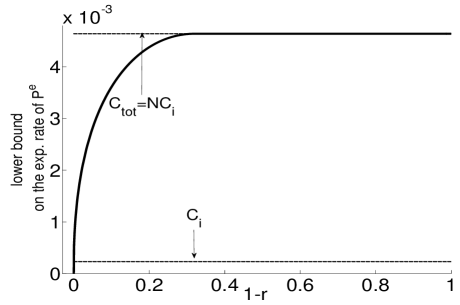
Figure 2: Lower bound on the exponential decay rate of the error probability (given by eqn. (52)) for the (generic) model in Section VI. The network has $N=20$ sensors, and ${\bf{C_{\mathrm{tot}}}}=0.0047$. The optimal rate (equal to ${\bf{C_{\mathrm{tot}}}}$) is achieved for $p\geq 0.29$.

We proceed by proving Theorem 6. We first set up the proof and state some auxiliary Lemmas. We first consider the probability of false alarm, $\alpha_{i,\mathrm{dis}}(k)=\mathbb{P}_{0}\left(x_{i}(k)>0\right)$, but the same conclusions will hold for $\beta_{i,\mathrm{dis}}(k)=\mathbb{P}_{1}\left(x_{i}(k)<0\right)$ also (See the Proof of Theorem 5.) We examine the family of Chernoff bounds on the probability of false alarm, parametrized by $\mu>0$, given by:

$$\alpha_{i,\mathrm{dis}}(k)\leq\mathbb{E}_{0}\left[e^{k\mu x_{i}(k)}\right]=:\mathcal{C}(k\mu),$$ (64)

where $\mathbb{E}_{l}\left[a\right]:=\mathbb{E}\left[a|H_{l}\right]$, $l=0,1.$ We then examine the conditions under which the best Chernoff bound falls below the negative of the Chernoff information, in the limit as $k\rightarrow\infty$. More precisely, we examine under which conditions the following inequality holds:

$$\limsup_{k\rightarrow\infty}\frac{1}{k}\log\mathcal{C}(k\mu)\leq-{\bf{C}_{\mathrm{tot}}}.$$ (65)

In subsequent analysis, we will use the following Lemmas, Lemma 7 and Lemma 8; proof of Lemma 7 is trivial, while proof of Lemma 8 is in the Appendix.

Lemma 7

Let $V$ be a $N\times N$ stochastic matrix and consider the matrix $\widetilde{V}=V-J$. Then, for all $i=1,...,N$, the following inequalities hold:

$$\sum_{l=1}^{N}|\widetilde{V}_{il}| \leq 2\frac{N-1}{N}<2$$ (66)

$$\sum_{l=1}^{N}|\widetilde{V}_{il}|^{2} \leq \frac{N-1}{N}<1.$$ (67)

Lemma 8

Let Assumption 4 hold. Then, the following inequality holds:

$$\mathbb{P}\left(\|\widetilde{\Phi}(k,j)\|>\epsilon\right)\leq\frac{N^{4}}{\epsilon^{2}}r^{k-j}.$$ (68)

When proving Theorem 6, we will partition the time interval from the first to $(k-1)$-th time step in windows of width $B$, for some integer $B\geq 1$. That is, we consider the subsets of consecutive time steps $\{k-B,k-B+1,...,k-1\}$, $\{k-2B,...,k-B-1\}$, $...$, $\{k-(\mathcal{J}-1)B,...,k-\mathcal{J}B-1\}$, $\{1,2,...,k-\mathcal{J}B-1\}$, where $\mathcal{J}$ is the integer part of $\frac{k-1}{B}$. (Note that the total number of these subsets is $\mathcal{J}+1$; each of these subsets contains $B$ time steps, except $\{1,2,...,k-\mathcal{J}B-1\}$ that in general has the number of time steps less or equal to $B$.) We then define the events $\mathcal{A}_{j}$, $j=1,...,\mathcal{J}+1$, as follows:

$$\mathcal{A}_{1} = \left\{\|\widetilde{\Phi}(k,k-B)\|\leq\epsilon\right\}$$ (69)

$$\mathcal{A}_{2} = \left\{\|\widetilde{\Phi}(k,k-B)\|>\epsilon\right\}\cap\left\{\|\widetilde{\Phi}(k,k-2B)\|\leq\epsilon\right\}$$

$$\vdots$$

$$\mathcal{A}_{j+1} = \left\{\|\widetilde{\Phi}(k,k-jB)\|>\epsilon\right\}\cap\left\{\|\widetilde{\Phi}(k,k-(j+1)B)\|\leq\epsilon\right\}$$

$$\vdots$$

$$\mathcal{A}_{\mathcal{J}} = \left\{\|\widetilde{\Phi}(k,k-(\mathcal{J}-1)B)\|>\epsilon\right\}\cap\left\{\|\widetilde{\Phi}(k,k-\mathcal{J}B)\|\leq\epsilon\right\}$$

$$\mathcal{A}_{\mathcal{J}+1} = \left\{\|\widetilde{\Phi}(k,k-\mathcal{J}B)\|>\epsilon\right\}.$$

It is easy to see that the events $\mathcal{A}_{j}$, $j=1,...,\mathcal{J}+1$, constitute a finite partition of the probability space $\Omega$ (i.e., each $\mathcal{A}_{i}$ and $\mathcal{A}_{j}$, $i\neq j$, are disjoint, and the union of $\mathcal{A}_{j}$’s, $j=1,...,\mathcal{J}+1$, is $\Omega$.)

By Lemma 8, the probability of the event $\mathcal{A}_{j}$, $j=1,...,\mathcal{J}+1$, is bounded from above as follows:

$$\mathbb{P}\left(\mathcal{A}_{j}\right)\leq\frac{N^{4}}{\epsilon^{2}}r^{(j-1)B}.$$ (70)

We will next explain the idea behind using the partition $\mathcal{A}_{j}$, $j=1,...,\mathcal{J}+1$. First, we state Lemma 9 that helps to understand this idea.

Lemma 9

Consider the random matrices $\widetilde{\Phi}(k,j)$ given by eqn. (23), and fix two time steps, $k$ and $j$, $k>j$. Suppose that the event $\mathcal{A}_{j}$ occurred. Then, for any $s\leq k-jB$, and for $i=1,...,N$:

$$\sum_{l=1}^{N}|[\widetilde{\Phi}(k,s)]_{il}| \leq N\sqrt{N}\epsilon$$ (71)

$$\sum_{l=1}^{N}|[\widetilde{\Phi}(k,s)]_{il}|^{2} \leq N\epsilon^{2}.$$ (72)

Proof.

See the Appendix. ∎

Consider now the partition $\mathcal{A}_{j}$, $j=1,...,\mathcal{J}+1$. Given that $\mathcal{A}_{j}$ occurred, the matrices $\Phi(k,s)$, for $s\leq k-jB$, are “$\epsilon$-close” to $J$ (in view of Lemma 9.) For $s>k-jB$, $\Phi(k,s)$ is not “$\epsilon$-close” to $J$, and thus we pass to the “worst case” as given by Lemma 7. (We may think of this as setting $\Phi(k,s)\approx I$.) Hence, given that $\mathcal{A}_{j}$ occurred, $x(k)$, in a crude approximation, behaves as:

$$x(k)\sim\frac{1}{k}\sum_{l=1}^{k-jB}J\eta(l)+\frac{1}{k}\sum_{l=k-jB+1}^{k}I\eta(l).$$

Then, by conditioning $x(k)$ on $\mathcal{A}_{j}$, $j=1,...,\mathcal{J}+1$, and by using the total probability (as with Theorem 5,) we express $P^{e}_{i,\mathrm{dis}}(k)$ in terms of the $j=1,...,\mathcal{J}+1$ “modes of decay” that correspond to $\mathcal{A}_{j}$, $j=1,...,\mathcal{J}+1$. Finally, we find the slowest among the $\mathcal{J}+1$ modes, as with Theorem 5. The difference compared to Theorem 5, however, is that here we work with the Chernoff bounds on $\alpha_{i,\mathrm{dis}}(k)$ and $P^{e}_{i,\mathrm{dis}}(k)$, rather than directly with $\alpha_{i,\mathrm{dis}}(k)$ and $P^{e}_{i,\mathrm{dis}}(k)$. After this qualitative description and after explaining the main idea behind the calculations, we proceed with the exact calculations, some of which are moved to the Appendix.

Proof of Theorem 6.

Consider the Chernoff bound on $\alpha_{i,\mathrm{dis}}(k)$ given by eqn. (64), and denote by $\overline{m}_{0}:=\max_{i=1,...,N}|[m_{\eta}^{(0)}]_{i}|$. We first express the Chernoff upper bound on $\limsup_{k\rightarrow\infty}\frac{1}{k}\log P^{e}_{i,\mathrm{dis}}(k)$ in terms of the “modes of decay,” similarly as in the Proof of Theorem 5. Namely, it can be shown (details are in the Appendix) that the following inequality holds:

$$\limsup_{k\rightarrow\infty}\frac{1}{k}\log\alpha_{i,\mathrm{dis}}(k) = \limsup_{k\rightarrow\infty}\frac{1}{k}\log P^{e}_{i,\mathrm{dis}}(k)$$

$$\leq \limsup_{k\rightarrow\infty}\frac{1}{k}\log\overline{\mathcal{C}}(k\mu)\overline{\delta}(k\mu),\,\,\forall\mu>0,\,\forall\epsilon\in(0,1),\,\,\forall B=1,2,...$$

where

$$\overline{\mathcal{C}}(k\mu) = \mathrm{exp}\left((k-1)(\frac{1}{2N^{2}}\sigma_{L}^{2}\mu^{2}+\frac{1}{N}m_{L}^{(0)}\,\mu)\right)$$ (74)

$$\overline{\delta}(k\mu) = \sum_{j=0}^{\mathcal{J}}\mathrm{exp}\left(|2\mu^{2}-\mu|\,\overline{m}\,\left\{2(j+1)B+(k-(j+1)B)N\sqrt{N}\epsilon\right\}\right)$$

$$\mathrm{exp}\left(\frac{\mu^{2}}{2}\,\|S^{\eta}\|\,\left\{(j+1)B+(k-(j+1)B)N\epsilon^{2}\right\}\right)\left(\frac{N^{4}\,r^{jB}}{\epsilon^{2}}\right).$$

Notice that the summands in eqn. (VI-A) are the “modes of decay” that correspond to the events $\mathcal{A}_{j+1}$, $j=1,...,\mathcal{J}+1$. Next, after bounding from above by “the slowest mode,” we get:

$$\overline{\delta}(k\mu) \leq \left(\mathcal{J}+1\right)\,\max_{j=0,...,\mathcal{J}}\,\mathrm{exp}\left(|2\mu^{2}-\mu|\,\overline{m}\,\left\{2(j+1)B+(k-(j+1)B)N\sqrt{N}\epsilon\right\}\right)$$ (76)

$$\mathrm{exp}\left(\frac{\mu^{2}}{2}\,\|S^{\eta}\|\,\left\{(j+1)B+(k-(j+1)B)N\epsilon^{2}\right\}\right)\left(\frac{N^{4}\,r^{jB}}{\epsilon^{2}}\right).$$ (77)

Introduce the variable $\theta=\theta(j)=\frac{jB}{k}$. We now replace the maximum over the discrete set $j=0,...,\mathcal{J}$, in eqn. (76) by the supremum over $j\in[0,\mathcal{J}]$, i.e., $\theta\in[0,1]$; we get:

$$\delta(k\mu) \leq \left(\mathcal{J}+1\right)\sup_{\theta\in[0,1]}\mathrm{exp}\left(|2\mu^{2}-\mu|\,\overline{m}\,\left\{2k\theta(1-N\sqrt{N}\epsilon)+B(2-N\sqrt{N}\epsilon)+kN\sqrt{N}\epsilon\right\}\right)$$

$$\mathrm{exp}\left(\frac{\mu^{2}}{2}\,\|S^{\eta}\|\,\left\{k\theta(1-N\epsilon^{2})+B(1-N\epsilon^{2})+k\epsilon^{2}\right\}\right)\left(\frac{N^{4}r^{jB}}{\epsilon^{2}}\right).$$

Taking the limsup as $k\rightarrow\infty$, and then letting $\epsilon\rightarrow 0$, we obtain the following inequality:

$$\limsup_{k\rightarrow\infty}\frac{1}{k}\log\mathcal{C}(k\mu) \leq \sup_{\theta\in[0,1]}\phi(\theta;\,\mu),\,\,\forall\mu>0$$ (79)

$$\phi(\theta;\,\mu) = \frac{1}{2N^{2}}\sigma_{L}^{2}\mu^{2}+\frac{1}{N}m_{L}^{(0)}\,\mu+2|2\mu^{2}-\mu|\overline{m}\theta+\frac{\mu^{2}}{2}\|S^{\eta}\|\theta+\theta\log r.$$ (80)

Eqn. (79) gives a family of upper bounds, indexed by $\mu>0$, on the quantity $\limsup_{k\rightarrow\infty}\frac{1}{k}\log\alpha_{i,\mathrm{dis}}(k)$; we seek the most aggressive bound, i.e., we take the infimum over $\mu>0$.

We first discuss the values of the parameter $r$, for which there exists a range $\mu\in[\frac{1}{2},\overline{\mu}]$ (where $\overline{\mu}$ is given by eqn. (62),) where the supremum in eqn. (79) is attained at $\theta=0$. It can be shown that this range is nonempty if and only if:

$$|\log r|>\frac{1}{8}\|S^{\eta}\|.$$ (81)

In view of eqns. (79), (80), and (81), we have the following inequality:

$$\limsup_{k\rightarrow\infty}\frac{1}{k}\log\mathcal{C}^{\prime}(k\mu)\leq\min_{\mu\in[\frac{1}{2},\overline{\mu}]}\left\{\frac{1}{2N^{2}}\sigma_{L}^{2}\mu^{2}+\frac{1}{N}m_{L}^{(0)}\,\mu\right\}.$$ (82)

The global minimum (on $\mu\in{\mathbb{R}}$) of the function $\mu\mapsto\frac{1}{2N^{2}}\sigma_{L}^{2}\mu^{2}+\frac{1}{N}m_{L}^{(0)}\,\mu$ is attained at $\mu^{\star}=N/2$; and it can be shown that it equals the negative of the Chernoff information $-{\bf{C_{\mathrm{tot}}}}=-\frac{1}{8}(m_{1}-m_{0})^{\top}S^{-1}(m_{1}-m_{0}).$ Thus, a sufficient condition for $\limsup_{k\rightarrow\infty}\frac{1}{k}\log\alpha_{i,\mathrm{dis}}(k)\leq\limsup_{k\rightarrow\infty}\frac{1}{k}\log\mathcal{C}^{\prime}(k\mu)\leq-{\bf{C_{\mathrm{tot}}}}$ is that $\mu^{\star}=\frac{N}{2}\in[\frac{1}{2},\overline{\mu}]$. By straightforward algebra, it can be shown that the latter condition translates into the following condition:

$${|\log r|}\geq\frac{1}{8}N^{2}\left(1+(1-\frac{1}{N})K\right)\|S^{\eta}\|.$$ (83)

The analysis of the upper bound on $\alpha_{i,\mathrm{dis}}(k)$ remains true for the upper bound on $\beta_{i,\mathrm{dis}}(k)$; hence, we conclude that, under condition (83), we have: $\limsup_{k\rightarrow\infty}\frac{1}{k}\log\beta_{i,\mathrm{dis}}(k)\leq-{\bf{C_{\mathrm{tot}}}}$. Thus, under the condition (83), the following holds:

$$\limsup_{k\rightarrow\infty}\frac{1}{k}\log P^{e}_{i,\mathrm{dis}}(k) = \max\left(\limsup_{k\rightarrow\infty}\frac{1}{k}\log\alpha_{i,\mathrm{dis}}(k),\,\limsup_{k\rightarrow\infty}\frac{1}{k}\log\beta_{i,\mathrm{dis}}(k)\right)\leq-{\bf{C_{\mathrm{tot}}}}.$$ (84)

On the other hand, by the Chernoff Lemma (Lemma 3,) we also know that

$$\liminf_{k\rightarrow\infty}\frac{1}{k}\log P^{e}_{i,\mathrm{dis}}(k)\geq-{\bf{C_{\mathrm{tot}}}}.$$ (85)

By eqns. (84) and (85), we conclude that $\lim_{k\rightarrow\infty}\frac{1}{k}\log P^{e}_{i,\mathrm{dis}}(k)=-{\bf{C_{\mathrm{tot}}}}$, for the values of $r$ that satisfy the condition (83). Hence, condition (83) is a sufficient condition for asymptotic optimality.

Consider now the values of $r$ such that:

$$\frac{1}{8}\|S^{\eta}\|<{|\log r|}<\frac{1}{8}N^{2}\left(1+(1-\frac{1}{N})K\right)\|S^{\eta}\|.$$ (86)

In this range, $\frac{1}{2}<\overline{\mu}<\mu^{\star}=N/2$, and the minimum of the function $\mu\mapsto\frac{1}{2N^{2}}\sigma_{L}^{2}\mu^{2}+\frac{1}{N}m_{L}^{(0)}\,\mu$ on $\mu\in[\frac{1}{2},\overline{\mu}]$ is attained at $\mu=\overline{\mu}$. Hence, for the values of $r$ in the range (86), we have the following bound:

$$\limsup_{k\rightarrow\infty}\frac{1}{k}\log P^{e}_{i,\mathrm{dis}}(k) = \max\left(\limsup_{k\rightarrow\infty}\frac{1}{k}\log\alpha_{i,\mathrm{dis}}(k),\,\limsup_{k\rightarrow\infty}\frac{1}{k}\log\beta_{i,\mathrm{dis}}(k)\right)$$ (87)

$$\leq \frac{1}{2N^{2}}\sigma_{L}^{2}\overline{\mu}^{2}+\frac{1}{N}m_{L}^{(0)}\,\overline{\mu}.$$ (88)

Finally, consider the values of $r$ such that the condition in (81) does not hold, i.e., $\frac{1}{8}\|S^{\eta}\|\geq{|\log r|}$. We omit further details, but it can be shown that, in this case, the supremum in eqn. (79) is attained at $\theta=0$ only for the values of $\mu$ in a subset of $[0,\frac{1}{2}]$; and it can be shown that $\limsup_{k\rightarrow\infty}\frac{1}{k}\log P^{e}_{i,\mathrm{dis}}(k)$ can be bounded as given by eqn. (61). ∎

VI-B Necessary condition for asymptotic optimality

We proceed with necessary conditions for asymptotic optimality, for the case when the sensors’ observations are spatially uncorrelated, i.e., the noise covariance $S=\mathrm{Diag}\left(\sigma_{1}^{2},...,\sigma_{N}^{2}\right)$. Denote by $E_{i}(k)$ the event that, at time $k$, sensor $i$ is connected to at least one of the remaining sensors in the network; that is,

$$E_{i}(k):=\left\{\max_{j=1,...,N,\,j\neq i}W_{ij}(k)>0\right\}.$$ (89)

Further, denote by $P_{i}(k)=P_{i}=\mathbb{P}(E_{i}(k))$ We have the following result.

Theorem 10 (Necessary condition for asymptotic optimality)

Consider the distributed detection algorithm in eqns. (18) and (19) with spatially uncorrelated sensors’ observations, and let Assumption 4 hold. Then, a necessary condition for the asymptotic optimality of distributed detection at sensor $i$ is:

$$|\log(1-P_{i})|>{\bf{C_{\mathrm{tot}}}}-{\bf{C}_{i}}.$$ (90)

Proof.

Consider $\alpha_{i,\mathrm{dis}}(k)$, but remark that the same conclusions will hold for $\beta_{i,\mathrm{dis}}(k)$, as $\alpha_{i,\mathrm{dis}}(k)=\beta_{i,\mathrm{dis}}(k).$ (See the proof of Theorem 5.) Further, using inequalities (7), we have:

$$\alpha_{i,\mathrm{dis}}(k) = \mathbb{P}_{0}\left(x_{i}(k)>0\right)$$ (91)

$$\geq \mathbb{P}_{0}\left(x_{i}(k)>0|\cap_{s=1}^{k}E_{i}(s)\right)\mathbb{P}\left(\cap_{s=1}^{k}E_{i}(s)\right)$$ (92)

$$\geq \frac{1}{\sqrt{2\pi}}\,\frac{\sqrt{2k}{\bf C}_{i}}{1+2k{\bf C}_{i}}e^{-k{\bf{C}_{i}}}(1-P_{i})^{k}.$$ (93)

Thus, we have that

$$\liminf_{k\rightarrow\infty}\frac{1}{k}\log\alpha_{i,\mathrm{dis}}(k)\geq-\left({\bf{C}_{i}}+|\log(1-P_{i})|\right).$$ (94)

On the other hand, we know that

$$\liminf_{k\rightarrow\infty}\frac{1}{k}\log P^{e}_{i,\mathrm{dis}}(k) \geq \liminf_{k\rightarrow\infty}\frac{1}{k}\log\alpha_{i,\mathrm{dis}}(k)\geq-{\bf{C}_{\mathrm{tot}}}.$$ (95)

The claim of Theorem 10 now follows from eqns. (94) and (95). ∎

VII Simulations

In this section, we corroborate by simulation examples our analytical findings on the asymptotic behavior of distributed detection over random networks. Namely, we demonstrate the “phase change” behavior of distributed detection with respect to the speed of network information flow, as predicted by Theorem 6. Also, we demonstrate that a sensor with poor connectedness to the rest of the network cannot be an optimal detector, as predicted by Theorem 10; moreover, its performance approaches the performance of an isolated sensor, i.e., a sensor that works as an individual detector, as connectedness becomes worse and worse.

Simulation setup. We consider a supergraph $G$ with $N=40$ nodes and $M=247$ edges. Nodes are uniformly distributed on a unit square and nodes within distance less than a radius $r$ are connected by an edge. As averaging weights, we use the standard time-varying Metropolis weights $W_{ij}(k)$, defined for $\{i,j\}\in E,i\neq j$, by $W_{ij}(k)=1/(1+\max(d_{i}(k),d_{j}(k)))$, if the link $\{i,j\}$ is online at time $k$, and 0 otherwise. The quantity $d_{i}(k)$ represents the number of neighbors (i.e., the degree) of node $i$ at time $k$. Also, $W_{ii}(k)=1-\sum_{j\in\Omega_{i}(k)}W_{ij}(k)$, for all $i$, and $W_{ij}(k)\equiv 0$, for $i\neq j$, $\{i,j\}\notin E$. The link failures are spatially and temporally independent. Each link $\{i,j\}\in E$ has the same probability of formation, i.e., the probability of being online at a time, $q_{ij}=q$. This network and weight model satisfy Assumption 4.

We assume equal prior probabilities, $\mathbb{P}(H_{0})=\mathbb{P}(H_{1})=0.5$. We set the $N\times 1$ signal vector under $H_{1}$ (respectively, $H_{0}$) to be $m_{1}=1$ (respectively, $m_{0}=0$.) We generate randomly the covariance matrix $S$, as follows. We generate: a $N\times N$ matrix $M_{S}$, with the entries drawn independently from $U[0,1]$–the uniform distribution on $[0,1]$; we set $R_{S}=M_{S}M_{S}^{\top}$; we decompose $R_{S}$ via the eigenvalue decomposition: $R_{S}=Q_{S}\Lambda_{S}Q_{S}^{\top}$; we generate a $N\times 1$ vector $u_{S}$ with the entries drawn independently from $U[0,1]$; finally, we set $S=\alpha_{S}\,Q_{S}\mathrm{Diag}(u_{S})Q_{S}^{\top}$, where $\alpha_{S}>0$ is a parameter. For the optimal centralized detector, we evaluate $P^{e}_{\mathrm{cen}}(k)$ by formula (6). For the distributed detector, we evaluate $P^{e}_{i,\mathrm{dis}}(k)$ by Monte Carlo simulations with 20,000 sample paths (20,000 for each hypothesis $H_{l}$, $l=0,1$) of the running consensus algorithm.

Exponential rate of decay of the error probability vs. the speed of information flow. First, we examine the asymptotic behavior of distributed detection when the speed of network information flow varies, i.e., when $r$ varies. (We recall that $r:=\lambda_{2}\left(\mathbb{E}\left[W(k)^{2}\right]\right)$.) To this end, we fix the supergraph, and then we vary the formation probability of links $q$ from 0 to 0.75. Figure 3 (bottom left) plots the estimated exponential rate of decay, averaged across sensors, versus $q$. Figure 3 (bottom right) plots the same estimated exponential rate of decay versus $1-r$. We can see that there is a “phase change” behavior, as predicted by Theorem 6. For $q$ greater than 0.1, i.e., for $1-r>0.25$, the rate of decay of error probability is approximately the same as for the optimal centralized detector ${\bf{C_{\mathrm{tot}}}}$–the simulation estimate of ${\bf{C_{\mathrm{tot}}}}$ is 0.0106. For $q<0.1$, i.e., for $1-r<0.25$, detection performance becomes worse and worse as $q$ decreases. Figure 3 (top) plots the estimated error probability, averaged across sensors, for different values of $q$. We can see that the curves are “stretched” for small values of $q$; after $q$ exceeds a threshold (on the order of $0.1$,) the curves cluster, and they have approximately the same slope (the error probability has approximately the same decay rate,) equal to the optimal slope.

Study of a sensor with poor connectivity to the rest of the network. Next, we demonstrate that a sensor with poor connectivity to the rest of the network cannot be an asymptotically optimal detector, as predicted by Theorem 10; its performance approaches the performance of an individual detector-sensor, when its connectivity becomes worse and worse. For $i$-th individual detector-sensor (no cooperation between sensors,) it is easy to show that the Bayes probability of error, $P^{e}_{i,\mathrm{no\,\,cooper.}}(k)$ equals: $P^{e}_{i,\mathrm{no\,\,cooper.}}(k)=\mathcal{Q}\left(\sqrt{k}\frac{m_{i,\mathrm{no\,\,cooper.}}}{\sigma_{\mathrm{i,no\,\,cooper.}}}\right),$ where $m_{i,\mathrm{no\,\,cooper.}}=\frac{1}{2}\frac{[m_{1}]_{i}^{2}}{S_{ii}}$, and $\sigma_{\mathrm{i,no\,\,cooper.}}^{2}=\frac{[m_{1}]_{i}^{2}}{S_{ii}}.$ It is easy to show that the Chernoff information (equal to $\lim_{k\rightarrow\infty}\frac{1}{k}\log P^{e}_{i,\mathrm{no\,\,cooper.}}(k)$) for sensor $i$, in the absence of cooperation, is given by $\frac{1}{8}\frac{[m_{1}]_{i}^{2}}{S_{ii}}$.

We now detail the simulation setup. We consider a supergraph with $N=35$ nodes and $M=263$ edges. We initially generate the supergraph as a geometric disc graph, but then we isolate sensor 35 from the rest of the network, by keeping it connected only to sensor 3. We then vary the formation probability of the link $\{3,35\}$, $q_{3,35}$, from 0.05 to 0.5 (see Figure 4.) All other links in the supergraph have the formation probability of 0.8. Figure 4 plots the error probability for: 1) the optimal centralized detection; 2) distributed detection at each sensor, with cooperation (running consensus;) and 3) detection at each sensor, without cooperation (sensors do not communicate.) Figure 4 shows that, when $q_{3,35}=0.05$, sensor 35 behaves almost as bad as the individual sensors, that do not communicate (cooperate) with each other. As $q$ increases, the performance of sensor 35 gradually improves.

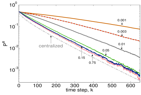
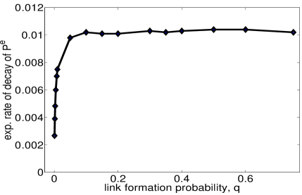
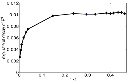
Figure 3: Monte Carlo estimate of the performance of distributed detection for different values of the link formation probability $q$. Top: Error probability averaged across $N$ sensors. Each line is labeled with the value of $q$; performance of centralized detection is plotted in gray. Bottom left (respectively, right): Estimated exponential rate of decay of the error probability vs. $q$ (respectively, $1-r$). Recall that $r:=\lambda_{2}\left(\mathbb{E}\left[W(k)^{2}\right]\right)$.

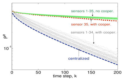
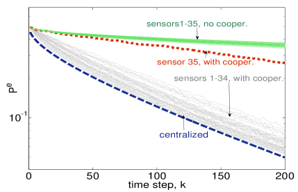
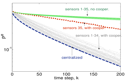
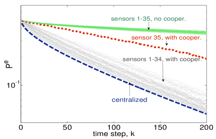
Figure 4: Error probability averaged across sensors for the optimal centralized detection, distributed detection at each sensor (with cooperation), and detection at each sensor, without cooperation. The formation probability $q_{3,35}$ of the link $\{3,35\}$ varies between 0.05 and 0.5: $q_{3,35}$=0.05 (top right); 0.2 (top left); 0.3 (bottom left); 0.5 (bottom right).

VIII Conclusion

We studied distributed detection over random networks when at each time step $k$ each sensor: 1) averages its decision variable with the neighbors decision variables; and 2) accounts on-the-fly for its new observation. We analyzed how asymptotic detection performance, i.e., the exponential decay rate of the error probability, depends on the random network connectivity, i.e., on the speed of information flow across network. We showed that distributed detection exhibits a “phase change.” Namely, distributed detection is asymptotically optimal, if the network speed of information flow is above a Chernoff information dependent threshold. When below the threshold, we find a lower bound on the achievable performance (the exponential rate of decay of error probability,) as a function of the network connectivity and the Chernoff information. Simulation examples demonstrate our theoretical findings on the asymptotic performance of distributed detection.

Appendix A Appendix

A-A Proof of inequalities (46)

Recall $\chi(l;k)$ in eqn. (41). Using eqn. (V), and noting that $(1-p)^{k-1}\geq p(1-p)^{k-1}$, we bound $\alpha_{i,\mathrm{dis}}(k)$ from below as follows:

$$\alpha_{i,\mathrm{dis}}(k) \geq \max_{l=0,...,k-1}\,\mathcal{Q}(\chi(l;k))\,p(1-p)^{k-l-1}$$ (96)

$$\geq \frac{1}{\sqrt{2\pi}}\,\max_{l=0,...,k-1}\,\frac{\chi(l;k)}{1+\chi(l;k)^{2}}e^{-\frac{1}{2}\chi(l;k)^{2}}\,p(1-p)^{k-l-1}$$ (97)

$$\geq \frac{1}{\sqrt{2\pi}}\,\frac{\sqrt{2k{\bf{C_{i}}}}}{1+2kN{\bf{C_{i}}}}\max_{l=0,...,k-1}e^{-\frac{1}{2}\chi(l;k)^{2}}\,p(1-p)^{k-l-1}$$ (98)

$$= \frac{1}{\sqrt{2\pi}}\,\frac{\sqrt{2k{\bf{C_{i}}}}}{1+2kN{\bf{C_{i}}}}\max_{l=0,...,k-1}p\,e^{-\frac{k{\bf{C_{\mathrm{tot}}}}}{1+(N-1)(1-\frac{l}{k})}-(k-l-1)|\log(1-p)|}$$ (99)

$$= \frac{1}{\sqrt{2\pi}}\,\frac{\sqrt{2k{\bf{C_{i}}}}}{1+2kN{\bf{C_{i}}}}\max_{j=0,...,k-1}p\,e^{-\frac{k{\bf{C_{\mathrm{tot}}}}}{1+(N-1)\frac{(j+1)}{k}}-j|\log(1-p)|}$$ (100)

$$= \frac{1}{\sqrt{2\pi}}\,\frac{\sqrt{2k{\bf{C_{i}}}}}{1+2kN{\bf{C_{i}}}}\max_{j=0,...,k-1}p\,e^{-k\,\phi(j;k)}.$$ (101)

Inequality in eqn. (97) is due to (7), equality in (100) is by letting $j=k-l-1,$ and equality in (101) is by definition of $\phi(j;k)$ in eqn. (44). Taking $\liminf_{k\rightarrow\infty}\frac{1}{k}\log\alpha_{i,\mathrm{dis}}(k)$, and using (36), (96)-(101) yields:

$$\liminf_{k\rightarrow\infty}\frac{1}{k}\log P^{e}_{i,\mathrm{dis}}(k) \geq \liminf_{k\rightarrow\infty}\frac{1}{k}\log\alpha_{i,\mathrm{dis}}(k)\geq-\limsup_{k\rightarrow\infty}\left\{\min_{j=0,...,k-1}\phi(j;k)\right\}.$$ (102)

Next, using eqn. (V), we bound $\mathbb{P}_{0}\left(x_{i}(k)>0\right)$ from above as follows:

$$\alpha_{i,\mathrm{dis}}(k) \leq k\,\max_{l=0,...,k-1}\,\mathcal{Q}(\chi(l;k))\,(1-p)^{k-l-1}$$ (103)

$$\leq k\,\frac{1}{\sqrt{2\pi}}\,\max_{l=0,...,k-1}\,\frac{1}{\chi(l;k)}e^{-\frac{1}{2}\chi(l;k)^{2}}\,(1-p)^{k-l-1}$$ (104)

$$\leq k\,\frac{1}{\sqrt{2\pi}}\,\frac{1}{\sqrt{2{\bf{C_{i}}}k}}\max_{l=0,...,k-1}e^{-\frac{1}{2}\chi(l;k)^{2}}\,(1-p)^{k-l-1}$$ (105)

$$= k\,\frac{1}{\sqrt{2\pi}}\,\frac{1}{\sqrt{2{\bf{C_{i}}}k}}\,\max_{l=0,...,k-1}\,\,e^{-\frac{k{\bf{C_{\mathrm{tot}}}}}{1+(N-1)(1-\frac{l}{k})}-(k-l-1)|\log(1-p)|}$$ (106)

$$= k\,\frac{1}{\sqrt{2\pi}}\,\frac{1}{\sqrt{2{\bf{C_{i}}}k}}\,\max_{j=0,...,k-1}\,e^{-\frac{k{\bf{C_{\mathrm{tot}}}}}{1+(N-1)\frac{j}{k}}-j|\log(1-p)|}$$ (107)

$$= k\,\frac{1}{\sqrt{2\pi}}\,\frac{1}{\sqrt{2{\bf{C_{i}}}k}}\,\max_{j=0,...,k-1}\,e^{-k\,\phi(j;k)}.$$ (108)

Inequality in (104) is due (7), and equality in (108) is by definition of $\phi(j;k)$ in eqn. (44). We complete the proof by noting that equality in (35) and inequalities (103)-(107) imply that:

$$\limsup_{k\rightarrow\infty}\frac{1}{k}\log P^{e}_{i,\mathrm{dis}}(k)=\limsup_{k\rightarrow\infty}\frac{1}{k}\log\alpha_{i,\mathrm{dis}}(k)\leq-\liminf_{k\rightarrow\infty}\left\{\min_{j\in\{0,...,k-1\}}\phi(j;k)\right\}.$$ (109)

A-B Proof of Lemma 8

Consider the random vector $z^{(i)}(k,j)=\widetilde{\Phi}(k,j)e_{i}$, which is equal to the $i$-th column of the matrix $\widetilde{\Phi}(k,j)$. First, by the Markov inequality, we have:

$$\mathbb{P}\left(\|z^{(i)}(k,j)\|>\epsilon\right)\leq\frac{1}{\epsilon^{2}}\mathbb{E}\left[z^{(i)}(k,j)^{\top}z^{(i)}(k,j)\right].$$ (110)

Now, we can bound $\mathbb{E}\left[z^{(i)}(k,j)^{\top}z^{(i)}(k,j)\right]$ as follows:

$$\mathbb{E}\left[z^{(i)}(k,j)^{\top}z^{(i)}(k,j)\right] = \mathbb{E}\left[\mathbb{E}\left[e_{i}^{\top}\widetilde{\Phi}(k-1,j)^{\top}\widetilde{W}(k-1)\widetilde{W}(k-1)\widetilde{\Phi}(k-1,j)e_{i}\,|\widetilde{W}(j),...,\widetilde{W}(k-2)\right]\right]$$ (111)

$$= \mathbb{E}\left[e_{i}^{\top}\widetilde{\Phi}(k-1,j)^{\top}\mathbb{E}\left[\widetilde{W}(k-1)\widetilde{W}(k-1)\right]\widetilde{\Phi}(k-1,j)e_{i}|\,\widetilde{W}(j),...,\widetilde{W}(k-2)\right]$$

$$\leq \|\mathbb{E}\left[\widetilde{W}(k-1)^{2}\right]\|\,\cdot\,\mathbb{E}\left[e_{i}^{\top}\widetilde{\Phi}(k-1,j)^{\top}\widetilde{\Phi}(k-1,j)e_{i}\right].$$

$$= r\,\mathbb{E}\left[z^{(i)}(k-1,j)^{\top}z^{(i)}(k-1,j)\right].$$

Now, bounding successively $\mathbb{E}\left[z^{(i)}(k-s,j)^{\top}z^{(i)}(k-s,j)\right]$ for $s=1,...,k-j$, as in eqn. (111), we obtain:

$$\mathbb{E}\left[z^{(i)}(k,j)^{\top}z^{(i)}(k,j)\right]\leq r^{k-j},$$ (112)

which yields (by eqn. (110):)

$$\mathbb{P}\left(\|z^{(i)}(k,j)\|>\epsilon\right)\leq\frac{1}{\epsilon^{2}}r^{k-j},\,i=1,...,N.$$ (113)

Now, observe that $\|z^{(i)}(k,j)\|_{1}\leq N\|z^{(i)}(k,j)\|$, and hence,

$$\mathbb{P}\left(\|z^{(i)}(k,j)\|_{1}>\epsilon\right)\leq\mathbb{P}\left(\|z^{(i)}(k,j)\|>\frac{\epsilon}{N}\right).$$

Further, in view of the matrix norm inequality $\|B\|\leq\sqrt{N}\|B\|_{1}$, we have:

$$\mathbb{P}\left(\|\widetilde{\Phi}(k,j)\|>\epsilon\right) \leq \mathbb{P}\left(\|\widetilde{\Phi}(k,j)\|_{1}>\frac{\epsilon}{\sqrt{N}}\right)=\mathbb{P}\left(\max_{i=1,...,N}\|z^{(i)}(k,j)\|_{1}>\frac{\epsilon}{\sqrt{N}}\right)$$

$$= \mathbb{P}\left(\cup_{i=1}^{N}\{\|z^{(i)}(k,j)\|_{1}>\frac{\epsilon}{\sqrt{N}}\right)\leq\sum_{i=1}^{N}\mathbb{P}\left(\|z^{(i)}(k,j)\|_{1}>\frac{\epsilon}{\sqrt{N}}\right)\leq\frac{N^{4}}{\epsilon^{2}}r^{k-j}.$$

A-C Proof of Lemma 9

First, note that, if $\mathcal{A}_{j}$ occurred, we have that:

$$\|\widetilde{\Phi}(k,s)\|\leq\epsilon,\,\forall s\leq k-jB,$$

since $\|\widetilde{\Phi}(k,s)\|=\|[\widetilde{\Phi}(k,k-jB)\widetilde{\Phi}(k-jB-1,s)\|\leq\|\widetilde{\Phi}(k,k-jB)\|\|\widetilde{\Phi}(k-jB-1,s)\|,$ and $\|[\widetilde{\Phi}(k,k-jB)\|\leq\epsilon$ and $\|\widetilde{\Phi}(k-jB-1,s)\|\leq 1.$ Inequality (71) holds true, because:

$$\sum_{l=1}^{N}|[\widetilde{\Phi}(k,s)]_{il}| \leq N\,\max_{i,l=1,...,N}|[\widetilde{\Phi}(k,s)]_{il}|,$$

and $\max_{i,l=1,...,N}|[\widetilde{\Phi}(k,s)]_{il}|\leq\sqrt{N}\,\|\widetilde{\Phi}(k,s)\|\leq\sqrt{N}\epsilon.$ Inequality (72) holds true, because, for $s\leq k-jB$,

$$\sum_{l=1}^{N}|[\widetilde{\Phi}(k,s)]_{il}|^{2}\leq\|\widetilde{\Phi}(k,s)\|_{F}^{2}\leq N\|\widetilde{\Phi}(k,s)\|^{2}=N\epsilon^{2}.$$

A-D Proof of eqn. (VI-A)

Consider the Chernoff bound on $\alpha_{i,\mathrm{dis}}(k)$, given by:

$$\mathcal{C}\left(k\mu\right) := {\mathbb{E}}_{0}\left[\mathrm{exp}\,\left(k\mu\,x_{i}(k)\right)\right]={\mathbb{E}}_{0}\left[\mathrm{exp}\,\left(k\lambda^{\top}x(k)\right)\right],$$ (114)

where $\lambda=\mu\,e_{i}$, $\lambda\in{\mathbb{R}}^{N}$.

Further, we have:

$$\mathcal{C}\left(k\mu\right) = {\mathbb{E}}_{0}\left[\mathrm{exp}\,\left(\lambda^{\top}\sum_{j=1}^{k-1}{\Phi}(k,j)\eta(j)+\,\lambda^{\top}\eta(k)\right)\right]$$

$$= {\mathbb{E}}_{0}\left[\mathrm{exp}\,\left(\lambda^{\top}\sum_{j=1}^{k-1}{\Phi}(k,j)\eta(j)\right)\right]\,{\mathbb{E}}_{0}\left[\mathrm{exp}\left(\lambda^{\top}\eta(k)\right)\right],$$

where the last equality holds because $\eta(k)$ is independent from $\eta(j)$ and $W(j)$, $j=1,...,k-1$. We will be interested in computing $\limsup_{k\rightarrow\infty}\frac{1}{k}\Lambda_{k}^{(l)}(k\,\mu)$, for all $\mu\in{\mathbb{R}}$; with this respect, remark that

$$\lim_{k\rightarrow\infty}\frac{1}{k}\log{\mathbb{E}}_{0}\left[\mathrm{exp}\left(\lambda^{\top}\eta(k)\right)\right]=0,$$

for all $\lambda\in{\mathbb{R}}^{N}$, because $\eta(k)$ is a Gaussian random variable and hence it has finite log-moment generating function at any point $\lambda$.

Thus, we have that $\limsup_{k\rightarrow\infty}\frac{1}{k}\log\mathcal{C}\left(k\mu\right)=\limsup_{k\rightarrow\infty}\frac{1}{k}\log\mathcal{C}^{\prime}(k\mu)$, where

$$\mathcal{C}^{\prime}(k\mu)={\mathbb{E}}_{0}\left[\mathrm{exp}\,\left(\,\lambda^{\top}\sum_{j=1}^{k-1}{\Phi}(k,j)\eta(j)\right)\right].$$

We thus proceed with the computation of $\mathcal{C}^{\prime}(k\mu)$. Conditioned on $W(1),W(2),...,W(k-1)$, the random variables $\lambda^{\top}\Phi(k,j)\eta(j)$, $j=1,...,k-1$, are independent; moreover, they are Gaussian random variables, as linear transformation of the Gaussian variables $\eta(j)$. Recall that $m_{\eta}^{(0)}$ and $S^{\eta}$ denote the mean and the covariance of $\eta(k)$ under hypothesis $H_{0}$. After conditioning on $W(1),W(2),...,W(k-1)$, using the independence of $\eta(j)$ and $\eta(s)$ $s\neq j$, and using the expression for the moment generating function of $\eta(j)$, we obtain successively:

$$\mathcal{C}^{\prime}(\mu) = \mathbb{E}\left[{\mathbb{E}}_{0}\left[\mathrm{exp}\,\left(\,\lambda^{\top}\sum_{j=1}^{k-1}{\Phi}(k,j)\eta(j)\right)\right]|W(1),...,W(k-1)\right]$$

$$= \mathbb{E}\left[{\mathbb{E}}_{0}\left[\Pi_{j=1}^{k-1}\mathrm{exp}\left(\,\lambda^{\top}\Phi(k,j)\eta(j)\right)\right]|W(1),...,W(k-1)\right]$$

$$= \mathbb{E}\left[\Pi_{j=1}^{k-1}\mathbb{E}\left[\mathrm{exp}\,\left(\,\lambda^{\top}\Phi(k,j)\,m_{\eta}^{(l)}\right)\mathrm{exp}\,\left(\frac{1}{2}\lambda^{\top}\Phi(k,j)^{\top}S^{\eta}\Phi(k,j)\lambda\right)\right]\right]$$

$$= \mathbb{E}\,\,[\Pi_{j=1}^{k-1}\,\,\mathrm{exp}\,\left(\,\lambda^{\top}\left(\widetilde{\Phi}(k,j)+J\right)\,m_{\eta}^{(0)}\right)$$

$$\mathrm{exp}\,\left(\frac{1}{2}\left(J+\widetilde{\Phi}(k,j)\right)^{\top}S^{\eta}\left(J+\widetilde{\Phi}(k,j)\right)\right)].$$

Denote further:

$$\delta(k\mu) := \mathbb{E}\mathrm{[\,}\mathrm{exp}\left(\lambda^{\top}\sum_{j=1}^{k-1}\widetilde{\Phi}(k,j)m_{\eta}^{(l)}\right)\,\mathrm{exp}\left(\frac{1}{2}\lambda^{\top}\left(\sum_{j=1}^{k-1}\widetilde{\Phi}(k,j)^{\top}S^{\eta}\widetilde{\Phi}(k,j)\right)\lambda\right)\,$$

$$\mathrm{exp}\left(\frac{1}{2}\lambda^{\top}JS^{\eta}\sum_{j=1}^{k-1}\widetilde{\Phi}(k,j)\lambda\right)\,\mathrm{exp}\left(\frac{1}{2}\lambda^{\top}\sum_{j=1}^{k-1}\widetilde{\Phi}(k,j)^{\top}S^{\eta}J\lambda\right)\,\mathrm{]},$$

$$\overline{\mathcal{C}}(k\mu) := \mathrm{exp}\left((k-1)\left(\lambda^{\top}Jm_{\eta}^{(l)}-\frac{1}{2}\lambda^{\top}JS^{\eta}J\lambda\right)\right),$$ (117)

where dependence on $H_{0}$ is dropped in the definition of $\delta(k\mu)$. Then, it is easy to see that $\mathcal{C}^{\prime}(k\mu)=\overline{\mathcal{C}}(k\mu)\delta(k\mu)$.

Recall the expressions for $v$, $m_{L}^{(0)}$ and $\sigma_{L}^{2}$ in eqns. (10), (12). After straightforward algebra, it can be shown that $\overline{\mathcal{C}}(k\mu)$ equals the expression in eqn. (74). Remak further that $\delta(k\mu)$ equals:

$$\delta(k\mu)=\mathbb{E}\left[\mathrm{exp}\left((\mu-\mu^{2})e_{i}^{\top}\sum_{j=1}^{k-1}\widetilde{\Phi}(k,j)m_{\eta}^{(0)}\right)\mathrm{exp}\left(\frac{\mu^{2}}{2}e_{i}^{\top}\sum_{j=1}^{k-1}\widetilde{\Phi}(k,j)S^{\eta}\widetilde{\Phi}(k,j)^{\top}\right)e_{i}\right].$$ (118)

Recall that $\overline{m}_{0}:=\max_{i=1,...,N}|[m_{\eta}^{(0)}]_{i}|$. Now, $\delta(k\mu)$ can be bounded from above as follows:

$$\delta(k\mu) \leq \mathbb{E}\left[\mathrm{exp}\left(|\mu-\mu^{2}|\,\overline{m}_{0}\sum_{j=1}^{k-1}\sum_{l=1}^{N}\,|[\widetilde{\Phi}(k,j)]_{il}|\right)\,\mathrm{exp}\left(\frac{\mu^{2}}{2}\|S^{\eta}\|\sum_{j=1}^{k-1}|[\widetilde{\Phi}(k,j)]_{il}]|^{2}\right)\right]$$

$$\leq \mathbb{E}\left[\mathrm{exp}\left(|\mu-\mu^{2}|\,\overline{m}_{0}\sum_{j=1}^{k}\sum_{l=1}^{N}\,|[\widetilde{\Phi}(k,j)]_{il}|\right)\,\mathrm{exp}\left(\frac{\mu^{2}}{2}\|S^{\eta}\|\sum_{j=1}^{k}|[\widetilde{\Phi}(k,j)]_{il}]|^{2}\right)\right].$$

Using Lemmas 9, 8 and 7, using the total probability with the partition $\mathcal{A}_{j}$, $j=1,...,\mathcal{J}+1$, we get the inequality (VI-A).

Appendix B Summary

References

- [1] R. Viswanatan and P. R. Varshney, “Decentralized detection with multiple sensors: Part I–fundamentals,” Proc. IEEE, vol. 85, pp. 54–63, January 1997.
- [2] J. F. Chamberland and V. Veeravalli, “Decentralized dectection in sensor networks,” IEEE Transactions on Signal Processing, vol. 51, no. 2, pp. 407–416, February 2003.
- [3] J. N. Tsitsiklis, “Decentralized detection,” Adv. Statis. Signal Processing, vol. 2, pp. 297–344, 1993.
- [4] R. S. Blum, S. A. Kassam, and H. V. Poor, “Decentralized detection with multiple sensors: Part II–advanced topics,” Proc. IEEE, vol. 85, pp. 64–79, January 1997.
- [5] S. Kar, S. A. Aldosari, and J. M. F. Moura, “Topology for distributed inference on graphs,” IEEE Transactions on Signal Processing, vol. 56, no. 6, pp. 2609 –2613, June 2008.
- [6] S. Kar and J. M. F. Moura, “Consensus based detection in sensor networks: topology design under practical constraints,” in Proc. Workshop Inf. Theory in Sensor Networks, Santa Fe, NM, June 2007.
- [7] P. Braca, S. Marano, V. Matta, and P. Willet, “Asymptotic optimality of running consensus in testing binary hypothesis,” IEEE Transactions on Signal Processing, vol. 58, no. 2, pp. 814–825, February 2010.
- [8] F. S. Cattivelli and A. H. Sayed, “Diffusion LMS-based detection over adaptive networks,” in Proc. Asilomar Conf. Signals, Systems and Computers, Pacific Grove, CA, October 2009.
- [9] ——, “Distributed detection over adaptive networks based on diffusion estimation schemes,” in Proc. IEEE SPAWC ’09, 10th IEEE International Workshop on Signal Processing Advances in Wireless Communications, Perugia, Italy, June 2009, pp. 61 –65.
- [10] D. Jakovetic, J. Xavier, and J. M. F. Moura, “Weight optimization for consenus algorithms with correlated switching topology,” IEEE Transactions on Signal Processing, vol. 58, no. 7, pp. 3788–3801, July 2010.
- [11] S. Boyd, A. Ghosh, B. Prabhakar, and D. Shah, “Randomized gossip algorithms,” IEEE Transactions on Information Theory, vol. 52, no. 6, pp. 2508–2530, June 2006.
- [12] C. G. Lopes and A. H. Sayed, “Diffusion least-mean squares over adaptive networks: formulation and performance analysis,” IEEE Transactions on Signal Processing, vol. 56, no. 7, pp. 3122 –3136, July 2008.
- [13] F. S. Cattivelli and A. H. Sayed, “Diffusion LMS strategies for distributed estimation,” IEEE Transactions on Signal Processing, vol. 58, no. 3, pp. 1035 –1048, March 2010.
- [14] I. D. Schizas, G. Mateos, and G. B. Giannakis, “Distributed LMS for consensus-based in-network adaptive processing,” IEEE Trans. on Signal Processing, vol. 57, no. 6, pp. 2365 –2381, June 2009.
- [15] ——, “Distributed recursive least-squares for consensus-based in-network adaptive estimation,” IEEE Trans. on Signal Processing, vol. 57, no. 11, pp. 4583 –4588, November 2009.
- [16] S. Kar, J. M. F. Moura, and K. Ramanan, “Distributed parameter estimation in sensor networks: Nonlinear observation models and imperfect communication,” August 2008, submitted for publication, 51 pages. [Online]. Available: arXiv:0809.0009v1 [cs.MA]
- [17] S. A. Kassam, Signal Detection in Non-Gaussian Noise. New York: Springer-Verlag, 1987.
- [18] D. Bajovic, D. Jakovetic, J. Xavier, B. Sinopoli, and J. M. F. Moura, “Distributed detection over time varying networks: large deviations analysis,” in 48th Allerton Conference on Communication, Control, and Computing, Monticello, IL, Oct. 2010.
- [19] T. M. Cover and J. A. Thomas, Elements of information theory. New York: John Wiley and Sons, 1991.
- [20] S. A. Aldosari and J. M. F. Moura, “Detection in sensor networks: the saddlepoint approximation,” IEEE Transactions on Signal Processing, vol. 55, no. 1, pp. 327–340, January 2007.
- [21] A. Dembo and O. Zeitouni, Large deviations techniques and applications. Boston, MA: Jones and Barlett, 1993.
- [22] H. L. V. Trees, Detection, Estimation, and Modulation Theory - Part l - Detection, Estimation, and Linear Modulation Theory. John Wiley and Sons, 2001.
- [23] P. Braca, S. Marano, and V. Matta, “Enforcing consensus while monitoring the environment in wireless sensor networks,” IEEE Transactions on Signal Processing, vol. 56, no. 7, pp. 3375–3380, July 2008.