Asymmetric 1+1-dimensional hydrodynamics in collision

Abstract

The possibility that particle production in high-energy collisions is a result of two asymmetric hydrodynamic flows is investigated, using the Khalatnikov form of the 1+1-dimensional approximation of hydrodynamic equations. The general solution is discussed and applied to the physically appealing “generalized in-out cascade” where the space-time and energy-momentum rapidities are equal at initial temperature but boost-invariance is not imposed. It is demonstrated that the two-bump structure of the entropy density, characteristic of the asymmetric input, changes easily into a single broad maximum compatible with data on particle production in symmetric processes. A possible microscopic QCD interpretation of asymmetric hydrodynamics is proposed.

I Introduction

The standard phenomenological description of heavy-ion reactions is based on the hydrodynamic evolution of the system, starting from rather early times. This approach allows to explain many aspects of data, e.g. the transverse momentum spectra and elliptic flow Hydr ; flor .

The hydro calculations mostly concentrate at the central rapidity region and therefore they often leave aside the problem of longitudinal dynamics. The usual approach for symmetric collisions ($e.g.$ for gold-gold collisions) is to consider a rapidity symmetric medium which, after some pre-equilbirium stage, evolves following the hydrodynamic equations till the freeze-out temperature. The investigated solutions of the hydrodynamic equations are naturally symmetric since they are obtained with initial conditions which are themselves rapidity-symmetric.

In the present paper we discuss a different hydrodynamic approach where, starting from asymmetric initial conditions, one considers asymmetric solutions of the hydrodynamic equations. The symmetry of the overall solution, in particular of the rapidity distribution of particles, is thus restored by the superposition of two conjugate asymmetric solutions. Such a situation has been advocated to explain (i) the forward-backward multiplicity correlations observed in nucleon-nucleon and nucleus-nucleus reactions bz ; bz1 ; bzw as well as (ii) the sign and magnitude of the directed flow observed in nucleus-nucleus collisions bw . It is also natural in some models wound ; wbz ; dpm ; fritjof describing the multiplicity distributions in p-p and gold-gold reactions. Finally, it is obviously necessary for an hydrodynamic description of the asymmetric reactions, e.g. deuteron-gold collision wbc .

For this scenario to be realized, one has to show that the hydrodynamic evolution is compatible with the existence of asymmetric components and with their possible combination to form a reasonable overall symmetric distribution. It is the goal of our paper to show that this is indeed the case. We use the simplified but informative framework of the (1+1)-dimensional approximation of the corresponding hydrodynamic flow. In this context we i) discuss the construction of asymmetric solutions, ii) show that the linear superposition of asymmetric components of the multiplicity distribution in rapidity is possible to construct in an hydrodynamic framework, more precisely of its (1+1)-dimensional approximation by the longitudinal entropy density as a function of rapidity.

It was shown long time ago by Khalatnikov khal that the hydrodynamic equations in (1+1) dimensions, considered first in the context of high-energy collisions by Landau Lan1 ; bi , can be linearized. This is achieved by passing from kinematic variables (position and time) into dynamic ones (temperature and rapidity). Recently this idea was developped in a modern context Beuf ; ps and used in the discussion of the longitudinal evolution of the symmetric solutions. The argument of the present paper extensively exploits these new developments and in particular the linearity property, which allows to consider the superposition of various solutions.

We shall discuss how one can obtain explicit solutions of the hydrodynamic equations which can be in phenomenological agreement with the two-source description in terms of the wounded constituent models wound ; wbz ; wbc . In doing so, we will more generally describe the full exact solution of the (1+1)-dimensional approximation of a perfect fluid flow. Finally, we shall speculate on the possible field-theoretical interpretation of our solutions in terms of early asymmetric thermalization in heavy-ion high-energy collisions.

The plan of our paper is the following: in section II we recall the derivation of the Khalatnikov equation. It allows for a general solution of the (1+1)-dimensional approximation of the perfect fluid flow which we derive in section III. From that general solution we discuss the existence of conservation laws as shown in IV, and then the definition of the initial conditions which are formulated in V. In section VI, we derive and discuss in detail the physically appealing family of solutions corresponding to the generalization of the “In-Out cascade ” scenario bj , where the space-time and momentum rapidities are taken equal at initial temperature. In the final section VII, we give our conclusions and discuss the possible microscopic QCD interpretation of asymmetric hydrodynamics.

II The Khalatnikov Equation

It is known khal ; bi that one can formulate the problem of (1+1) hydrodynamic evolution with a linear equation for a suitably defined potential. In this section we briefly recall these results, recasting the calculations in the light-cone kinematic variables, as used in Beuf ; ps

$$z^{\pm}=z^{0}\pm z^{1}\equiv t\pm z=\tau e^{\pm\eta}\;\Rightarrow\;\left(\frac{\partial}{\partial z^{0}}\pm\frac{\partial}{\partial z^{1}}\right)=2\frac{\partial}{\partial z^{\pm}}\ (\equiv 2\partial_{\pm}),$$ (1)

where $\tau=\sqrt{z^{+}z^{-}}\$ is the proper time and $\eta=\frac{1}{2}\ln({z^{+}}/{z^{-}})$ is the space-time rapidity of the fluid. We also introduce the dynamical variables: $y,$ the energy-momentum rapidity variable and $\theta,$ the logarithm of the inverse temperature, defined as

$$y=\log u^{+}=-\log u^{-}\ ;\quad\quad\theta=\log({T_{0}}/{T})\ ,$$ (2)

where $u^{\pm}=\log(u^{0}\pm u^{1})$ are the light-cone components of the fluid velocity and $T_{0}$ some given fixed temperature. We shall choose it to be the initial temperature of the plasma. Since plasma cools during the evolution we have always $\theta>0$.

Using thermodynamic relations, one can recombine the two relativistic hydrodynamic equations coming from the conservation of energy-momentum in (1+1) dimension, into two equivalent ones having a direct physical interpretation khal .

(i) The relation

$$\partial_{+}\left(e^{-\theta+y}\right)=\partial_{-}\left(e^{-\theta-y}\right).$$ (3)

implies the existence of a hydrodynamic potential $\Phi(z^{+},z^{-})$ such that:

$$\partial_{\mp}\Phi(z^{+},z^{-})\equiv T_{0}\ e^{-\theta\pm y}=u^{\pm}T,$$ (4)

meaning that the flow derives from a kinematic potential.

(ii) The second independent equation

$$\partial_{+}\left(u^{+}s\right)+\partial_{-}\left(u^{-}s\right)=0$$ (5)

corresponds to the conservation of entropy along the flow.

In order to combine usefully eqs.(4) and (5), one introduces the Khalatnikov potential khal

$$\chi(\theta,y)\equiv\Phi(z^{+},z^{-})-z^{-}u^{+}T-z^{+}u^{-}T\ ,$$ (6)

where $z^{\pm}$ are now considered as functions of $(\theta,y)$. This is called the hodograph transformation expressing the hydrodynamic equations as a function of the dynamical variables ($\theta,y$) $via$ the Legendre transform (6). Using the standard differential relations of a Legendre transform, the kinematic variables are recovered from the Khalatnikov potential by the equations

$$z^{\pm}(\theta,y)=\frac{1}{2T_{0}}\ e^{\theta\pm y}\ \left(\partial_{\theta}\chi\pm\partial_{y}\chi\right).$$ (7)

The Khalatnikov potential has the remarkable property khal ; bi ; ps ; Beuf to verify a $linear$ partial differential equation which takes the form

$$c^{2}_{s}\,\partial_{\theta}^{2}\chi(\theta,y)-\left[1-c_{s}^{2}\right]\partial_{\theta}\chi(\theta,y)-\partial^{2}_{y}\chi(\theta,y)=0\ .$$ (8)

In (8), $c_{s}$ (denoted also $1/\sqrt{g}$ for further convenience) is the speed of sound in the fluid, which will be considered as a constant in the present study.

The Khalatnikov equation has been originally derived khal for the potential (6) and with applications to specific problems. But its range of applicability appears to be much wider. Indeed, the transformation of a nonlinear problem in terms of the kinematic variables into a linear one in terms of dynamic variables has tremendous advantages, as we shall see further. It applies to other quantities than the Khalatnikov potential; It allows to obtain new solutions by arbitrary linear combinations of known ones. Furthermore, primitive integrals and derivatives of solutions are also solutions, as shown in ps .

In order to illustrate the powerfulness of this method, let us observe that if $\chi(\theta,y)$ is solution of (8), then the potential $\Phi,$ defined through (4), but now expressed in terms of the hydrodynamic variables through (7), reads

$$\Phi(\theta,y)\equiv\Phi\{z_{+}(\theta,y),z_{-}(\theta,y)\}=\chi(\theta,y)+\partial_{\theta}\chi(\theta,y),$$ (9)

and thus it verifies also the Khalatnikov equation (8). As a direct consequence, the physical entropy flow as a function of rapidity also verifies (8). Indeed, one has Beuf (see also milekhin )

$$\frac{dS}{dy}(\theta,y)=2s_{0}T_{0}^{g}\ e^{-(g-1)\theta}\ \partial_{\theta}\Phi(\theta,y)\ ,$$ (10)

where we use the thermodynamic relation $s=s_{0}T^{g}=s_{0}T_{0}^{g}e^{-g\theta}$ for the overall, temperature-dependent, entropy density of a perfect fluid, recalling that by definition $c_{s}^{2}\equiv 1/g$. Since the entropy distribution gives approximately the predicted distribution of produced particles, eq.(10) provides a rather direct link between solutions of the Khalatnikov equation and observables. Thus (10) plays a central role in the present study.

Before going further, it proves useful to use appropriately rescaled variables allowing to put the Khalatnikov equation (8) in a simple and symmetric form. Introducing

$$t=\frac{g-1}{2}\ \theta\,\;\;\;\;\;x=\frac{g-1}{2\sqrt{g}}\ y\ ,$$ (11)

redefining $\chi(t,x)$ as a function of these reduced variables, and introducing the auxiliary function

$$Z(t,x)=e^{-t}\chi(t,x)\ ,$$ (12)

the Khalatnikov equation (8) takes the simple form

$$(\partial_{t}^{2}-\partial_{x}^{2})Z=Z$$ (13)

III The solution

Equation (13) is nothing else than the $1\!+\!1$-dimensional Klein-Gordon equation (called also the Telegraphic equation bateman ). The solution, for arbitrary (Cauchy) initial conditions at $t=0$, is solu

$$Z=\frac{1}{2}\left\{f(x+t)+f(x-t)\right\}+\frac{1}{2}\int_{x-t}^{x+t}\!ds\ h(s)\ I_{0}(r)+\frac{1}{2}\int_{x-t}^{x+t}\!ds\ f(s)\ \frac{\partial I_{0}(r)}{\partial t}$$ (14)

where

$$r=\sqrt{t^{2}-(s-x)^{2}}$$ (15)

and $I_{0}(r)$ is the modified Bessel function of the first kind.

According to Eqns. (9,10) and using (12) we can express the entropy distribution as

$$\frac{dS}{dy}=\frac{s_{0}T_{0}^{g}}{2}(g\!-\!1)e^{-t}\left\{(g+1)Z+2g\partial_{t}Z+(g-1)\partial_{t}^{2}Z\right\}\ .$$ (16)

One also has for the kinematic flow variables, using (7),

$$\tau=\frac{g\!-\!1}{2\sqrt{2}T_{0}}\ e^{\frac{g\!+\!1}{g\!-\!1}\ t}\sqrt{\left(Z+\partial_{t}Z\right)^{2}-c_{s}^{2}(\partial_{x}Z)^{2}};\;\;\;\eta=y+\frac{1}{2}\log\left\{\frac{Z+\partial_{t}Z+c_{s}\partial_{x}Z}{Z+\partial_{t}Z-c_{s}\partial_{x}Z}\right\}\ .$$ (17)

IV Conservation laws

To discuss the conservation laws we observe that it is possible to rewrite the general solution (14) in the form of an inverse Laplace transform, implying the identity abr

$$\Theta[t\!-\!|s\!-\!x|]I_{0}\left[\sqrt{t^{2}\!-\!(s\!-\!x)^{2}}\ \right]=\int_{c-i\infty}^{c+i\infty}\frac{d\gamma}{2\pi i}\frac{1}{\sqrt{\gamma^{2}-1}}\ e^{\gamma t-|s-x|\sqrt{\gamma^{2}-1}}$$ (18)

with $\Re e\ c>1$. Inserting this expression into (14), reversing the order of integrations and using the derivative relation

$$\frac{\partial}{\partial t}\left\{\Theta[t\!-\!|s\!-\!x|]I_{0}\left[\sqrt{t^{2}\!-\!(s\!-\!x)^{2}}\right]\right\}=\Theta[t\!-\!|s\!-\!x|]\frac{\partial}{\partial t}I_{0}\left[\sqrt{t^{2}\!-\!(s\!-\!x)^{2}}\right]+\delta[t\!-\!|s\!-\!x|]$$ (19)

one sees that the solution (14) can be written in the form

$$Z=\frac{1}{2}\int_{c-i\infty}^{c+i\infty}\frac{d\gamma}{2\pi i}\frac{e^{-\gamma t}}{\sqrt{\gamma^{2}-1}}\int_{-\infty}^{+\infty}ds\ [h(s)+\gamma f(s)]\ e^{-|s-x|\sqrt{\gamma^{2}-1}}.$$ (20)

It is not too difficult to show that (18) and (19) do indeed satisfy (13).

Starting from (20) one can derive a sum rule:

$$\int_{-\infty}^{+\infty}\!dxZ(t,x)=e^{-t}\int_{-\infty}^{+\infty}\!dx\ \frac{h(x)+f(x)}{2}-e^{t}\int_{-\infty}^{+\infty}\!dx\ \frac{h(x)-f(x)}{2}$$ (21)

where the integral

$$\int_{-\infty}^{\infty}\!dx\ Z(t,x)=\int_{c-i\infty}^{c+i\infty}\frac{d\gamma}{2\pi i}\frac{e^{\gamma t}}{\gamma^{2}-1}\int_{-\infty}^{+\infty}\!dx[h(x)+\gamma f(x)]$$ (22)

was evaluated using the residue theorem.

From (21) one can obtain two conservation laws:

$$e^{-t}\ \int_{-\infty}^{+\infty}\!dx\left[Z(t,x)+\partial_{t}Z(t,x)\right]=\int_{-\infty}^{+\infty}\!dx\ \frac{h(x)+f(x)}{2};$$ (23)

$$e^{t}\ \int_{-\infty}^{+\infty}\!dx\ \left[Z(t,x)-\partial_{t}Z(t,x)\right]=\int_{-\infty}^{+\infty}\!dx\ \frac{f(x)-h(x)}{2}.$$ (24)

Comparing (23) with (16) one can see that (23) implies that the total entropy is independent of $t$, i.e. independent of the ratio $T_{0}/T$. This means that the total entropy does not change during the evolution of the system. Moreover, since the freeze-out temperature may safely be considered as constant, it also means that the total entropy is proportional to $T_{0}^{g}$, as expected from rules of thermodynamics.

Interestingly enough, equation (24) furnishes another independent conservation law for the $1\!+\!1$-dimensional hydrodynamics of a perfect fluid. Probably due to the (1+1)-dimensional origin of the Khalatnikov equation, it would be interesting to know its physical interpretation. We checked the validity of both conservation laws in our numerical applications.

V Initial conditions

To discuss the consequences of the Khalatnikov eq., one has to determine, in terms of physical quantities, (i) initial conditions at $t=0$ (i.e. the functions $f(x)$ and $h(x)$) and (ii) the final value of $t$ at which the solution is to be evaluated. To this end we observe that at $t=0$ we obtain from (14)

$$Z(x)=f(x);\;\;\;\partial_{t}Z(x)=h(x);\;\;\;\partial^{2}_{t}Z=f^{\prime\prime}(x)+f(x)\ .$$ (25)

Introducing these formulae into (16) and (17) we have

$$\left.\frac{dS}{dy}\right|_{t=0}=gs_{0}T_{0}^{g}\left\{f(x)+h(x)+\frac{g-1}{2g}f^{\prime\prime}(x)\right\}\ ,$$ (26)

and

$$\tau_{0}(x)=\frac{1}{2T_{0}}\sqrt{\left\{[f(x)+h(x)]^{2}-[f^{\prime}(x)]^{2}/g\right\}};\;\;\;\eta_{0}(x)=\frac{2\sqrt{g}}{g-1}\ x\left(=y\right)+\frac{1}{2}\log\left\{\frac{f(x)+h(x)+c_{s}f^{\prime}(x)}{f(x)+h(x)-c_{s}f^{\prime}(x)}\right\}$$ (27)

where $(\tau_{0}(x),\eta_{0}(x))=\left.(\tau,\eta)\right|_{t=0}$.

To determine the final value of $t$ we have to fix the physical conditions at which the system changes into free-moving hadrons. It seems reasonable to assume that this happens at a fixed freeze-out temperature $T=T_{f}$. Then the final value of $t$ at which the physical solution should be evaluated is

$$t\to t_{f}=\log\frac{T_{0}}{T_{f}}+\log\frac{g\!-\!1}{2}\ .$$ (28)

We thus conclude that the initial temperature $T_{0}$ is needed to be defined in order to determine the final value of $t$ at which the physical solution is to be evaluated.

If $T_{0}$ is fixed then eq.(27) determines the proper time $\tau_{0}(x)$ at which the evolution starts and eq.(17) gives the proper time at which freeze-out takes place. To illustrate these features, in the next section we discuss a simple while physically appealing case, when $f(x)=0.$

VI Generalized in-out cascade

When $f(x)\equiv 0$, we have

$$Z=\frac{1}{2}\int_{x-t}^{x+t}\!ds\ h(s)\ I_{0}(\sqrt{t^{2}-(s-x)^{2}})\ .$$ (29)

with $t=t_{f}$ given by (28). Using this we also derive

$$\partial_{t}Z=\frac{1}{2}\{h(x\!+\!t)+h(x\!-\!t)\}+\frac{1}{2}\int_{x-t}^{x+t}\!ds\ h(s)\ \frac{\partial I_{0}(\sqrt{t^{2}-(s-x)^{2}})}{\partial t}$$ (30)

and

$$\partial_{t}^{2}Z=\frac{1}{2}\{h^{\prime}(x\!+\!t)-h^{\prime}(x\!-\!t)\}+\frac{t}{4}\left\{h(x\!+\!t)+h(x\!-\!t)\right\}+\frac{1}{2}\int_{x-t}^{x+t}\!ds\ h(s)\frac{\partial^{2}I_{0}(r)}{\partial t^{2}}$$ (31)

where we have used the formula

$$\frac{\partial I_{0}(r)}{\partial t}=I_{0}^{\prime}(r)\frac{t}{r}=\frac{tI_{1}(r)}{r}\rightarrow\frac{t}{2}{\rm\ when\ }r\to 0\ .$$ (32)

To see the physical meaning, we observe that when (29) is introduced into (7) one has

$$z^{\pm}(0,x)=\left\{\frac{g-1}{4T_{0}}\ h(x)\right\}\ u^{\pm};\;\;\;\;\Rightarrow\;\;\;\;\eta_{0}=y|_{t=0}\ ,$$ (33)

i.e. at $t=0$ the position $z^{\pm}$ is aligned along the velocity $u^{\pm}$. This can be interpreted as a generalization of the in-out cascade bj for which $\eta=y$ at all temperatures leading to boost-invariance hydrodynamics (or “Bjorken flow”). In our generalized in-out cascade, the relation $\eta=y$ is valid at the initial stage $t=0$ only. The boost invariance is violated (unless $h(x)$ is a constant) because the ratio $u/z$ depends on rapidity.

Eqs. (26) and (27) reduce to

$$\left.\frac{dS}{dy}\right|_{t=0}=\frac{s_{0}T_{0}^{g}}{2}\ h(x);\;\;\;\tau_{0}(x)=\frac{g-1}{4T_{0}}\ h(x);\;\;\;\eta_{0}=y\ .$$ (34)

To show a specific example, let us consider the following simple parametrization of the intitial entropy distibution at $T=T_{0}(t=0):$

$$h(x)=(1-x/x_{max})^{a}\ (1+x/x_{max})^{b}\ \exp{[(x/x_{max}-1)/c}]\ ,$$ (35)

where $x_{max}=t_{max}=\log T_{0}/T_{f}$ and $a,b,c$ are constants characterizing the initial entropy profile. In the plots we keep $a=b=2$ for simplicity and vary $c=\{0.3,0.4,0.5\}.$

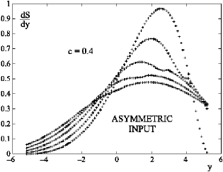
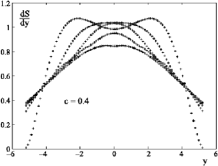
Figure 1: $dS/dy$ for 5 growing values of $T_{0}/T_{f}=2^{k},k=0\to 4.$ $Left$: asymmetric one-component model; $Right$: symmetric two-component model. Here one takes $c=0.4$ (see text).

In Fig. 1, we display the resulting curves corresponding to the entropy $vs.$ rapidity distribution for 5 temperature values from the initial one to the freeze-out, namely for $T_{0}/T_{f}=2^{k},k=0\to 4.$ It can be seen that the hydrodynamic diffusion towards the tails of the one-component distribution (Fig. 1, left) is responsible for the smooth disappearance of the two-bump initial structure of the symmetrized distribution (Fig. 1, right) obtained by linear combination. The initial bump structure may be easily modified by changing the form of $h(x)$. This also modifies the evolution of the entropy distribution as shown in Fig.2.

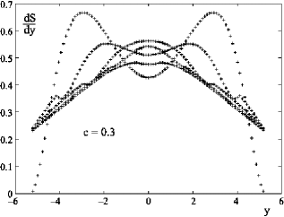
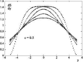
Figure 2: Two-component $dS/dy$ for 5 growing values of $T_{0}/T_{f}=2^{k},k=0\to 4.$ $Left$: strongly bumped asymmetric input ($c=.3$); $Right:$ weakly bumped asymmetric input ($c=.5$).

It is also interesting to display some characteristic kinematic features of the flow solutions, both for the asymmetric and symmetric cases. Note that for those features, the symmetric configuration is $not$ a linear symmetrized combination of both components, due to the nonlinear character of the solution for kinematics (17). The $\tau$-distribution can be found in Fig. 3.

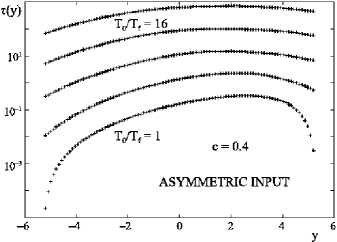
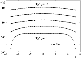
Figure 3: Two-component proper-time distribution $\tau(x)$ for 5 growing values of $T_{0}/T_{f}=2^{k},k=0\to 4.$
$Left$: asymmetric one-component model; $Right:$ symmetric two-component model. Here one takes $c=0.4$.

Concerning the kinematic properties of the flow one can make the following comments.

First, as seen in the left panel of Fig.3, the distribution of proper times is significantly asymmetric. This means that, at any given $y\neq 0$, the two asymmetric components freeze-out at different proper times. This observation supports the idea that the sets of particles emitted by these two components are indepedent of each other (as required by the analysis of the long-range correlations bz ; bz1 ; bzw ).

If the two components are mixed up during the evolution, the freeze-out time is very different from the previous case. This is illustrated in the right panel of Fig.3 where one sees that, for a fixed temperature, the proper-time of the symmetric solution is close to constant in the central rapidity region, at least at not-too-large values of the ratio $T_{0}/T_{f}$. This is consistent with an approximate Bjorken flow bj . One also observes that $\tau(y)$ increases with increasing ratio $T_{0}/T_{f}$, as expected. Note that the curves for $T_{0}/T_{f}=1$ (the lowest ones in the Fig.3) represent the proper time at which the evolution starts.

We have also evaluated how much the space-time rapidity $\eta$ deviates from $y$ along the evolution. As shown in Fig. 4, we have found that the difference $\eta-y$ is small, of the order of at most few %. This confirms that the the evolution of the system we are considering is close to the Bjorken flow. All these features show that the flow is rather smooth and laminar. We observe a slight but systematic tendency to obtain $\eta\lesssim y,$ growing for large space-time rapidities, which indicates that the flow is going “outwards”, i.e. moving apart on both sides from a kinematic tangential flow which would correspond to the original “In-Out” cascade mechanism.

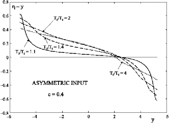
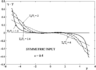
Figure 4: $\eta\!-\!y$ for 5 growing values of $T_{0}/T_{f}$, marked in the figure; ($c=.4$). Note that $\eta-y=0$ for $T_{0}/T_{f}=1$. $Left$: asymmetric one-component model; $Right$: symmetric two-component model.

VII Summary and comments

In summary, we have investigated the longitudinal hydrodynamic evolution of a one-dimetional perfect fluid (with a constant sound velocity). Using the Khalatnikov equation in the light-cone variables, derived earlier Beuf ; ps , the problem could be reduced to the discussion of solutions of the (1+1) Klein-Gordon equation (called also “Telegraphic equation” bateman ). Using the well-known general form of these solutions, we discussed their consequences in case the initial conditions are asymmetric, as necessary e.g. for proton-nucleus or asymmetric nuclei collisions and as also suggested by some models wbc ; wbz ; dpm ; fritjof .

We have studied in some detail only one simple but physically appealing example which can be considered as a natural generalization of the Bjorken flow bj which, as is well-known, give a boost-invariant expansion of the fluid. To relax boost-invariance, we assume that although at the beginning of expansion $z^{\pm}\sim u^{\pm}$ (c.f. (33)), the proportionality coefficient is not a constant (as in the case of Bjorken flow) but it is a function of $y$. This violates boost invariance and thus, among other rapidity configurations, it is possible to study asymmetric ones. The results of our study may be synthesized as follows:

i) Our main conclusion is that the hydrodynamic expansion broadens rather effectively the asymmetric bumpy structure of the entropy density (taken for the input). Consequently, for symmetric collisions (as, e.g. $p\!-\!p$ or $Pb\!-\!Pb$) where the asymmetric input has to be symmetrized, the two-bump structure of the entropy density, characteristic of the asymmetric input, changes easily into a single broad maximum. Thus we have shown that even a strongly asymmetric input can be compatible with data on particle production in symmetric processes.

ii) We have also studied the properties of the flow. The most important consequence of the initial conditions violating boost invariance is that the proper time at which evolution begins is not constant but depends on rapidity. In the simple case we considered, it is even downright proportional to the initial entropy density. Also the freeze-out time depends on rapidity, although the evolution has the tendency to smooth out this dependence.

iii) The rapidity dependence of $\tau_{0}$ and $\tau_{f}$ is especially interesting for strongly asymmetric initial conditions. In this case also the proper time is small in the region of small density and large in the region of large density. Consequently, if two asymmetric sources are present (as is the case for symmetric collisions) they freeze out at different times (except at c.m. rapidity close to 0). Therefore one may expect that they produce two bunches of particles which are indepenent of each other.

iv) We have also studied the evolution of the difference $\eta\!-\!y$ (which vanishes at $t=0$ in our simple example). It turns out that this difference remains small (below of 2-3 % of $y$) throughout the evolution (except at the very edge of phase-space where it may reach 10 %). Thus we conclude that the flow has tendency to be laminar and smooth, not very different from the Bjorken picture. It shows some systematic tendency to behave “outwards” i.e. moving apart on both sides from a kinematic tangential flow which would correspond to the original “In-Out” cascade mechanism.

v) As an interesting by-product, we have found two general identities valid for the (1+1)-dimensional approximation, corresponding to conservation laws along the temperature (and thus proper-time) evolution of the flow. One of them, see eq.(23), can be interpreted as the conservation of the full entropy. The other one, see eq.(24), up to our knowledge is new, and still asks for a physical interpretation.

Let us add a comment on the microscopic interpretation of our results for high-energy heavy ion collisions where the hydrodynamic set-up proved strikingly pertinent for the description of the Quark-Gluon Plasma phase of QCD Hydr ; flor . It is indeed extraordinary that hydrodynamics describes successfully and almost unambiguously this complicated process, belonging to the strongly coupled regime of QCD of which one does not know yet a microscopic description (although the string theory gives useful indications through the gauge/gravity duality in a kinematic collisional framework string , but for yet only supersymmetric gauge field theories).

As is well-known, the application of hydrodynamic description to heavy ion collisions requires a rather rapid thermalization of the system of quark and gluons created in the collision. This is not easy to reconcile with the idea that this system is described by perturbative QCD which is the usual scenario considered in this context. The perturbative QCD evolution of the wave-function of a boosted projectile generates a set of soft quantum fluctuations (gluons and $q\!-\!\bar{q}$ pairs) which develop as a virtual cascading process. This is revealed, for instance, when these a priori virtual fluctuations become observables, as in the case of the “hump-backed plateau” dg generated by a jet. Similarly, such virtual fluctuations play an important role in the theoretical understanding of deep-inelastic reactions. The problem arises because this system, considered as the initial state of the incident nuclei is highly anisotropic, therefore its thermalization after the collision is difficult and would require relatively long time.

Eventually, however, if the energy is sufficiently large, the soft fluctuations are dense enough in phase-space to interact and eventually lead to a saturation mechanism sat grouping them around some energy-dependent virtuality called the saturation scale. Therefore there is a possibility that, due to soft interactions which are long range in time, such a system thermalizes (at least approximately) already before the compound system created by the collision takes place. This is a possible model of the initial conditions we considered in the paper. It naturally requires asymmetric initial conditions.

To conclude, our investigation shows that the longitudinal hydrodynamic expansion of the system created in a high-energy collision may significantly influence the original rapidity distribution of partons in the colliding projectiles. It is therefore important to study this effect in more detail to obtain a reliable information on hadron structure at high energies.

Acknowledgements

This investigation was supported in part by the grant N N202 125437 of the Polish Ministry of Science and Higher Education (2009-2012). R.P. wants to thank the Institute of Physics for hospitality during the initial and final stages of the present work.

References

-
(1)
See, for instance,
P. F. Kolb and U. W. Heinz,
[arXiv: nucl-th/0305084];
T. Hirano, Acta Phys. Polon. B 36, 187 (2005);
P. Huovinen and P. V. Ruuskanen, Ann. Rev. Nucl. Part. Sci. 56, 163 (2006). - (2) For a recent review, see W.Florkowski, Phenomenology of Ultra-Relativistic Heavy Ion Collisions, World Scientific (2010).
- (3) A. Bzdak, Acta Phys. Pol. B41 (2010) 151.
- (4) A.Bzdak, Acta Phys. Pol. B41 (2010) 2471; Acta Phys. Pol. B40 (2009) 2029; Phys. Rev. C80 024906(2009).
- (5) A.Bzdak and K.Wozniak, Phys. Rev. C81 (2010) 034908.
- (6) P.Bozek and I.Wyskiel, Phys. Rev. C81 (2010) 054902; P.Bozek, Acta Phys. Pol. B41 (2010) 837.
- (7) A.Bialas, Bleszynski and W.Czyz, Nucl. Phys. B111 (1976) 461.
- (8) A. Bialas and A.Bzdak, Acta Phys. Pol. B38 (2007) 159; Phys. Lett. B649 (2007) 263; Phys. Rev. C77 (2008) 034908. For a review, see A.Bialas, J.Phys. G35 (2008) 044053.
- (9) A.Capella, C.I.Tan, A.Sukhatme and J.Tran Than Van, Phys. Rep. 236 (1994) 225.
- (10) B.Anderson, G.Gustafson and B.Nilsson-Almqvist, Nucl.Phys. B281 (1987) 289.
- (11) A.Bialas and W.Czyz, Acta Phys. Pol. B36 (2005) 905.
- (12) I.M.Khalatnikov, Zh.Eksp. Teor. Fiz. 26 529 (1954) (in Russian). For an English version, see Ref.bi , with a correction of the equation for the potential.
- (13) L. D. Landau, Izv. Akad. Nauk Ser. Fiz. 17, 51 (1953) (in Russian). [English translation: Collected Papers of L. D. Landau, edited by D. ter Haar (Gordon and Breach, New-York, 1968)].
-
(14)
S. Z. Belenkij and L. D. Landau,
Nuovo Cim. Suppl. 3S10 (1956) 15
[Usp. Fiz. Nauk 56 (1955) 309];
L. D. Landau, with S. Z. Belenkij, Collected Papers of L. D. Landau, edited by D. ter Haar (Gordon and Breach, New-York, 1968), Paper # 88, page 665 (the derivation of Khalatnikov’s solution is not given in Nuovo Cimento’s version). - (15) G. Beuf, R. Peschanski and E. N. Saridakis, Phys. Rev. C 78, 064909 (2008).
- (16) R. Peschanski and E. N. Saridakis, arXiv:1006.1603 [hep-th], to be published in Nucl.Phys.A.
- (17) J. D. Bjorken, Phys. Rev. D 27, 140 (1983).
- (18) A. Bialas, R. A. Janik and R. B. Peschanski, Phys. Rev. C 76, 054901 (2007).
- (19) G.A.Milekhin, Zh. Eksp. Teor. Fiz. 35, 1185 (1958) [Sov. Phys. JETP 35, 829 (1959)].
- (20) See e.g., H. Bateman, Partial Differential Equations of Mathematical Physics, Cambridge University Press (Cambridge, 1932), p.75.
- (21) See, for instance, T. Myint-U, Partial Differential Equations of mathematical Physics, Elsevier (1972), page 65 (up to the straightforward substitution of Bessel functions .)
- (22) M.Abramowitz and I.A.Stegun, Handbook of Mathematical Functions, Dover (1965), eqs. 29.3.93 and 29.2.2.
-
(23)
R. A. Janik and R. B. Peschanski,
Phys. Rev. D 73, 045013 (2006);
S. Bhattacharyya, V. E. Hubeny, S. Minwalla and M. Rangamani, JHEP 0802, 045 (2008). - (24) A.Bialas, Phys. Lett. B466 (1999) 301.
- (25) A.Bialas, M.Chojnacki and W.Florkowski, Phys. Lett. B661 (2008) 325.
- (26) W.Florkowski and R.Ryblewski, Acta Phys. Pol. B40 (2009) 2843; J.Phys. G37 (2010) 094023; R.Ryblewski and W.Florkowski, Acta Phys. Pol. Supp. 3 (2010) 557; Phys. Rev. C82 (2010) 024903;
- (27) Y. L. Dokshitzer, V. A. Khoze, A. H. Mueller and S. I. Troian, Basics of Perturbative QCD, Ed. Frontieres (1991), Gif-sur-Yvette, France (1991) 274 p., see Chapter 7 and references therein.
-
(28)
For a review and extended list of references, see
E. Iancu and R. Venugopalan, arXiv:hep-ph/0303204.