Abstract

The Darboux transformation operator technique in differential and integral forms is applied to the generalized Schrödinger equation with a position-dependent effective mass and with linearly energy-dependent potentials. Intertwining operators are obtained in an explicit form and used for constructing generalized Darboux transformations of an arbitrary order. A relation between supersymmetry and the generalized Darboux transformation is considered. The method is applied to generation of isospectral potentials with additional or removal bound states or construction of new partner potentials without changing the spectrum, i.e. fully isospectral potentials. The method is illustrated by some examples.

I Introduction

The problem of exact solvability of the Schrödinger equation has been extensively considered since the beginning of quantum mechanics Schr . A factorization technique was introduced by Schrödinger and was used to solve the harmonic oscillator, the hydrogen atom, the Kepler motion. It should be noted that factorization is closely connected with the Darboux transformation Darboux and the supersymmetry approach introduced by Witten in quantum mechanics Witten . Many interesting exactly solvable models have been constructed for Schrödinger equation using the Darboux and Bargmann transformation techniques Bagrov -Suz93 . Many advances have been made in the field of classifying quantum mechanical potentials according to their symmetry properties and in the area of different applications of exactly solvable models in quantum mechanics, in particular, in atomic and nuclear physics, in statistical mechanics Junker -Suz93 . Potentials of Bargmann- type and corresponding exact solutions can be obtained from the integral equations of the inverse scattering problem in the Gelfand-Levitan Gelfand and Marchenko approaches Marchenko with the degenerate kernels of the transformation operator. The differential Darboux transformations (or the method of itertwining) are closely related to supersymmetry and have a variety of applications in different fields of physics. The technique of iterated integral operators for Schrödinger equation is based on the integral Gelfand-Levitan and Marchenko equations (see e.g. Levitan ). The differential and integral approaches of obtaining exactly solvable equations are very close to each other, but sometimes the differential method is more convenient and sometimes the integral method is preferable. In particular, the integral form of transformations is used for construction of phase-equivalent potentials. Suggested in Scripta84 ; Suz85 generalized Darboux and Bargmann transformations permit construction of exactly solvable potentials for variable values of energy ${\cal E}$ and angular momentum $l$. The transformations in differential and integral forms were considered and it was shown how to construct the phase-equivalent potentials. Later on, this approach was generalized on the Schrödinger equation with weighted energy Suz93 and recently Acta the intertwining technique has been applied to construct exactly solvable potentials for this equation. The Schrödinger equation with energy-dependent potentials is widely used in nuclear physics, helium clusters and metal clusters Feshbach -Arias .

In the last few years the research efforts on the topic of algebraic methods have been considerably intensified Morrow -gener due to the rapid development of nanoelectronics, the basic elements of which are low-dimensional structures such as quantum wells, wires, dots and superlattices Goser ; physE . For investigation of nonuniform semiconductors, in which the carrier effective mass depends on position, the generalized Schrödinger equation with position-dependent effective mass is used Bastard . One of the most important problems of quantum engineering is the construction of multi-quantum well structures possessing desirable spectral properties. The technique of intertwining relations or Darboux transformations allows one to model quantum well potentials with a given spectrum. Although Darboux transformations are applicable to the position-dependent mass Schrödinger equation Plastino ; Milanov ; suz-shul ; Roy2 , the Schrödinger equation with weighted energy Acta and the generalized Schrödinger equation with position-dependent mass and weighted energy gener ; ss-JPA , however, their applications are very complicated for realization and there remain many problems to study. Nowadays there is a great interest to generate Hamiltonians with a prescribed energy spectrum. However, these problems are worth investigated for all cases of the generalized Schrödinger equations except for the standard Schrödinger equation ( see e.g. Chadan -matveev ).

In this paper we will focus on Darboux transformations of an arbitrary order applied to the generalized Schrödinger equation with a position-dependent mass and energy-dependent potentials. These generalized Darboux transformations include all known cases: Darboux transformations for the Schrödinger equation with the position-dependent mass, the case with linearly energy-dependent potentials as well as Darboux transformations for the conventional Schrödinger equation. It is known that Darboux transformations and supersymmetry are recovered for the standard Schrödinger equation. Here, we consider interrelations between supersymmetry and Darboux transformations for the generalized Schrödinger equation, establish a correspondence between the spaces of solutions to the initial and transformed equations. We show how the procedure can be used for generating families of Hamilltonians with a predetermined spectrum, removing or adding new bound states. Darboux transformations for the generalized Schrödinger equation are considered in the differential and integral forms. It should be noted, the integral transformations can be important for generation of new potentials completely isospectral to a given initial one without changing the spectrum and for construction of Hamilltonians differing by one bound state. A correspondence between the first- and second-order differential Darboux transformations and the integral ones is established. To explain our findings, we consider a few different applications of our approach and show how it is possible to generate completely isospectral potentials or to construct potentials with addition or moving of bound states from the spectrum of the initial Hamiltonian. We analyze the influence of the distances between the energy levels on the shape of potentials, which can be very complex. We construct asymmetric double well and even triple well potentials for the effective mass Schrödinger equation.

The paper is organized as follows. Section 2 is devoted to the generalized Darboux transformation of the first-order and corresponding supersymmetry formalism. In Section 3 we construct chains of generalized Darboux transformations by iteration of first-order Darboux transformations. Furthermore, we derive relations for potentials and solutions, obtained within the higher order Darboux transformations, in terms of potentials and solutions of the initial equations with no use of ones for the intermediate equations. In Section 4 we derive transformations in an integral form and establish relationship with differential Darboux transformations, afterwards we consider totally isospectral potentials. In Section 5 we illustrate our generalized transformations by concrete examples.

II The intertwining relations and supersymmetry

As it is well known, Darboux transformations (or supersymmetry) in nonrelativistic quantum mechanics allows one to produce Hamiltonians whose spectra can differ in one bound state. Recently gener , we have considered the first-order Darboux transformation for the Schrödinger equation with a position-dependent mass and weighted energy

$$-\left[\frac{d}{dx}\left(\frac{1}{m(x)}\right)\frac{d}{dx}\right]\phi(x)+v(x)\phi(x)=q(x){\cal E}\phi(x)~{}.$$ (1)

Here $m(x)$ stands for the particle’s effective mass, $q(x)$ and $v(x)$ denote the potentials, $\phi(x)$ is the wave function and ${\cal E}$ denotes the real-valued energy and we use atomic units. In this section we will briefly describe the method of intertwining operators of the first-order, then we will analyze the supersymmetry and the $n$th order transformations.

II.1 The first-order Darboux transformations

Consider two generalized Schrödinger equations

$${\cal H}\phi={\cal E}\phi~{},~{}~{}~{}{\cal H}=-\frac{1}{q(x)}\left[\frac{d}{dx}\left(\frac{1}{m(x)}\right)\frac{d}{dx}\right]+\frac{v(x)}{q(x)}~{},$$ (2)

$$\widetilde{\cal H}\widetilde{\phi}={\cal E}\widetilde{\phi}~{},~{}~{}~{}\widetilde{\cal H}=-\frac{1}{q(x)}\left[\frac{d}{dx}\left(\frac{1}{m(x)}\right)\frac{d}{dx}\right]+\frac{\widetilde{v}(x)}{q(x)}~{},$$ (3)

where Hamiltonians ${\cal H}$ and $\widetilde{\cal H}$ differ only in potentials $v$ and $\widetilde{v}$. In the conventional intertwining technique for the Schrödinger equation two one-dimensional Hamiltonians ${\cal H}=-\partial_{xx}+v$ and $\widetilde{\cal H}=-\partial_{xx}+\widetilde{v}$ and corresponding solutions $\phi$ and $\widetilde{\phi}$ are related by means of differential operator ${\cal L}$

$${\cal L}{\cal H}=\widetilde{\cal H}{\cal L}~{},$$ (4)

$$\widetilde{\phi}~{}=~{}{\cal L}~{}\phi~{}.~{}~{}~{}~{}~{}~{}$$ (5)

As it is known, the method of intertwining differential operators provides an universal approach to generating new exactly solvable equations shabat ; pavlov . We expand the intertwining relations on our generalized equation in order to determine the intertwining operator ${\cal L}$, a new potential and solutions of transformed equation (3) assuming that the solutions to the initial equation (2) are known. We seek for the intertwiner ${\cal L}$ in the form of a linear, first-order differential operator

$${\cal L}=A(x)+B(x)d/dx,$$ (6)

where the coefficients $A$ and $B$ are to be determined. To this end we insert (6) and the explicit form of the Hamiltonians ${\cal H}$ and $\widetilde{\cal H}$ into the intertwining relation (4) and apply it to the solution $\phi$ of (2). Assuming the linear independence of derivative operators of different order $d^{k}/dx^{k},~{}k=0,1,2,3$, we obtain the following system of equations for $A,~{}B$ and $\widetilde{v}$

$$\frac{2}{q~{}m}~{}B{~{}^{\prime}}~{}=~{}B~{}\left(\frac{1}{q~{}m}\right)^{\prime}~{},$$ (7)

$$\frac{2}{m}~{}A{{}^{\prime}}+\frac{1}{m}~{}B{~{}^{\prime\prime}}+\left(\frac{1}{m}\right)^{\prime}B{~{}^{\prime}}-B~{}q~{}\left[\frac{1}{q}\left(\frac{1}{m}\right)^{\prime}\right]^{\prime}~{}=~{}B~{}\left({\widetilde{v}}-{v}\right),$$ (8)

$$\frac{1}{m}~{}A{{}^{\prime\prime}}+\left(\frac{1}{m}\right)^{\prime}A{{}^{\prime}}+B~{}q\left(\frac{v}{q}\right)^{\prime}~{}=A~{}({\widetilde{v}}-v)~{},$$ (9)

where the prime denotes differentiation with respect to $x$ and arguments have been omitted. From (7) it follows

$$B=\frac{\beta}{\sqrt{q~{}m}}~{},$$ (10)

where $\beta$ is an arbitrary constant of integration. Equations (8) and (9) allow us to determine the potential ${\widetilde{v}}$ and the function $A$. Multiplying (8) by $A$ and (9) by $B$ and subtracting the resulting equations we obtain the equation with respect to $A$

$$-\frac{A{{}^{\prime\prime}}}{q~{}m}+\left(\frac{2A{{}^{\prime}}}{q~{}m~{}B}+\frac{B~{}{{}^{\prime\prime}}}{q~{}m~{}B}+\frac{1}{q}\left(\frac{1}{m}\right)^{\prime}\frac{B~{}{{}^{\prime}}}{B}-\left[\frac{1}{q}\left(\frac{1}{m}\right)^{\prime}\right]^{\prime}\right)A-B\left(\frac{v}{q}\right)^{\prime}-\frac{1}{q}\left(\frac{1}{m}\right)^{\prime}A{{}^{\prime}}=0.$$ (11)

In order to solve this equation, we introduce a new auxiliary function $K$ defined by $K=A/B$. Taking (10) into account, after simplification we arrive at the following nonlinear equation

$$\frac{d}{dx}\left[\frac{1}{q~{}m}\left(-K^{{}^{\prime}}+K^{2}\right)\right]-\frac{d}{dx}\left(\frac{v}{q}\right)-\frac{d}{dx}\left[\frac{1}{q}\left(\frac{1}{m}\right)^{\prime}~{}K\right]=0~{},$$

from which the generalized Riccati equation follows

$$\frac{1}{q~{}m}\left(-K^{{}^{\prime}}+K^{2}\right)-\frac{v}{q}-\frac{1}{q}\left(\frac{1}{m}\right)^{\prime}K=-\lambda,$$ (12)

where $\lambda$ is an arbitrary integration constant. Equation (12) turns into the conventional Riccati equation in particular cases of $m=const$ and $q=const$. With $B$ from (10) and $A=K/B$ the potential $\widetilde{v}$ can be expressed from (8) in terms of $K$ and known potentials $v$, $m$ and $q$

$$\widetilde{v}=v+2\sqrt{\frac{q}{m}}\frac{d}{dx}\frac{K}{\sqrt{q~{}m}}-\sqrt{\frac{q}{m}}\frac{d}{dx}\left[\frac{1}{q}\frac{d}{dx}\left(\sqrt{\frac{q}{m}}~{}\right)\right].$$ (13)

The potential $\widetilde{v}$ will be finally determined after finding the function $K$ from the Riccati equation (12), that can be linearized and integrated by introducing an auxiliary function ${\cal U}={\cal U}(x)$

$$K=-\frac{{\cal U}^{~{}^{\prime}}}{{\cal U}}.$$ (14)

Assuming that ${\cal U}$ is twice continuously differentiable and substituting (14) in (12) we get the equation

$$-\frac{1}{m}~{}{\cal U^{~{}^{\prime\prime}}}-\left(\frac{1}{m}\right)^{\prime}{\cal U}^{~{}^{\prime}}+v~{}{\cal U}=q~{}\lambda~{}{\cal U}~{},$$ (15)

which is identical to the initial equation (2) at ${\cal E}=\lambda$. Since the solutions of (2) with the given potentials $v$, $q$ and $m$ are known at all energies ${\cal E}$, hence we know the solution ${\cal U}$. Once ${\cal U}$ is given, the function $K$ is calculated via (14), which in turn determines $A$ by means of $A=BK$ and (10)

$$A=-\frac{1}{\sqrt{q~{}m}}\frac{{\cal U}^{~{}^{\prime}}}{{\cal U}}.$$

The constant of integration $\beta$ has been taken to one. By insertion of $K$ in (13) we obtain the explicit form of the transformed potential

$$\widetilde{v}=v-2\sqrt{\frac{q}{m}}\frac{d}{dx}\left[\frac{1}{\sqrt{q~{}m}}\frac{{\cal U}^{~{}^{\prime}}}{{\cal U}}\right]-\sqrt{\frac{q}{m}}\frac{d}{dx}\left[\frac{1}{q}\frac{d}{dx}\left(\sqrt{\frac{q}{m}}~{}\right)\right],$$ (16)

Finally, the intertwiner ${\cal L}$ and the transformation solution $\widetilde{\phi}$ are determined from (6) and (5), respectively

$${\cal L}=\frac{1}{\sqrt{q~{}m}}\left(\frac{d}{dx}+K\right)=\frac{1}{\sqrt{q~{}m}}\left[\frac{d}{dx}-\frac{{\cal U}^{~{}^{\prime}}}{{\cal U}}\right]~{},$$ (17)

$$\widetilde{\phi}~{}=~{}{\cal L}\phi=\frac{1}{\sqrt{q~{}m}}\left[\frac{d}{dx}-\frac{{\cal U}^{~{}^{\prime}}}{{\cal U}}\right]\phi~{}.$$ (18)

From (16) - (18) it follows that the transformed potential $\widetilde{v}$, the intertwiner ${\cal L}$ and solutions $\widetilde{\phi}$ depend not only on the potential $v$ but also on the additional potentials $m$ and $q$. It is easy to check that all expressions reduce to the well known ones for the Schrödinger equation if potential functions $m$ and $q$ are taken to be constant. When $q=const$ or $m=const$ we get first-order Darboux transformations for position-dependent mass Schrödinger equation suz-shul or for Schrödinger equation with weighted energy Acta as particular cases of our approach.

Solutions at the energy of transformation. Note that relation (18) connects the solutions of two equations (2) and (3) at an arbitrary energy except for solutions at energy of transformation, ${\cal E}=\lambda$. Evidently, at ${\cal E}=\lambda$ the action of Darboux transformation (17) on the function ${\cal U}$ and on functions $\phi$ linearly dependent to ${\cal U}$ gives us ${\cal L}{\cal U}=0$. In order to obtain a solution of the transformed equation (3) at energy $\lambda$, we replace ${\cal U}$ by a linearly independent solution $\widehat{\cal U}$

$$\widehat{\cal U}={\cal U}\int_{x_{0}}^{x}dx^{\prime}\frac{m(x^{\prime})}{|{\cal U}(x^{\prime})|^{2}}.$$ (19)

The limits of integration depend on the boundary conditions. The direct substitution $\widehat{\cal U}$ into (15) shows that $\widehat{\cal U}$ really solves the generalized Schrödinger equation. The action of ${\cal L}$ on the function $\widehat{\cal U}$ gives us a solution $\eta$ of the transformed equation (3) at energy $\lambda$

$$\eta={\cal L}\widehat{\cal U}=\sqrt{\frac{m}{q}}~{}\frac{1}{{\cal U}}~{}.$$ (20)

By using the generalized Liouville formula (19) once more, one can get a second solution $\widehat{\eta}$ of (3) at energy $\lambda$. For this ${\cal U}$ is replaced by $\eta$ in (19) and with (20) we get

$$\widehat{\eta}=\eta\int_{x_{0}}^{x}dx^{\prime}\frac{m(x^{\prime})}{|\eta(x^{\prime})|^{2}}=\sqrt{\frac{m}{q}}~{}\frac{1}{{\cal U}}\int_{x_{0}}^{x}dx^{\prime}q(x^{\prime})|{\cal U}(x^{\prime})|^{2}.$$ (21)

Hence, the knowledge of all solutions of the initial equation (2) provides the knowledge of all solutions of the transformed equation (3), including the solutions at energy of transformation. Notice that if ${\cal U}$ replies to the bound state of ${\cal H}$, then the function $\eta$ defined by (20) at the energy of transformation $\lambda$ cannot be normalized. Such bound state is excluded from the spectrum of ${\cal H}$. Therefore, the Hamiltonians ${\cal H}$ and $\widetilde{\cal H}$ are isospectral except for the bound state with energy $\lambda$, which is removed from the spectrum of ${\cal H}$.

II.2 Supersymmetry

Now we consider the generalization of the supersymmetric formalism (SUSY) on the generalized Schrödinger equation (1) and show how one can construct a Hamiltonian with an additional bound state by using supersymmetry. As it is well known, the SUSY algebra provides a relation between superpartner Hamiltonians, which can be presented in a factorized form in terms of Darboux transformation operators ${\cal L}$ and its adjoint ${\cal L}^{\dagger}$. In our case the scalar product of functions is defined by not the standard way $(f,\chi)$ but with the weight of $q$: $(f,\chi)_{q}=\int f^{*}(x)q(x)\chi(x)$. In this case instead of operator $D^{+}=(CQ)^{+}=Q^{+}C^{+}$ it is necessary to consider the operator $D^{\dagger}=q^{-1}D^{+}q$. Therefore, the operator ${\cal L}^{{\dagger}}$ adjoint to ${\cal L}=A+Bd/dx$ is determined as ${\cal L}^{\dagger}=q^{-1}\left(A-Bd/dx-dB/dx\right)q$. After simplification we arrive at

$${\cal L}^{{\dagger}}=\frac{1}{\sqrt{q~{}m}}\left(-\frac{d}{dx}+K\right)-\frac{1}{q}\frac{d}{dx}\sqrt{\frac{q}{m}}~{}$$ (22)

and the operator ${\cal L}^{{\dagger}}$ satisfies the intertwining relation

$${\cal H}{\cal L}^{{\dagger}}={\cal L}^{{\dagger}}\widetilde{\cal H}\,.$$ (23)

The generalized Schrödinger equations (2) and (3) can then be written as one single matrix equation in the form

$$\left(\begin{array}[]{cc}{\cal H}-\lambda&0\\ 0&\widetilde{\cal H}-\lambda\end{array}\right)\left(\begin{array}[]{c}\phi\\ \tilde{\phi}\end{array}\right)=0.$$ (28)

On defining $H_{s}=$ diag$({\cal H},\widetilde{\cal H})$ and $\Phi=(\phi,\tilde{\phi})^{T}$, the above matrix Schrödinger equation (28) can be written as

$$[H_{s}-\lambda I]~{}\Phi=0,$$ (29)

where $I$ is the $2\times 2$ unity matrix. Similar to the case of the standard Schrödinger equation, we define two supercharge operators $Q$, $Q^{\dagger}$ as follows:

$$Q=\left(\begin{array}[]{cc}0&0\\ {\cal L}&0\end{array}\right)~{},\qquad Q^{\dagger}=\left(\begin{array}[]{cc}0&{\cal L}^{\dagger}\\ 0&0\end{array}\right),$$ (34)

where ${\cal L}$ and ${\cal L}^{\dagger}$ are the operators given by (17) and (22), respectively. One can show that the matrix Hamiltonian $H_{s}$, as given in (29), satisfies the following conditions:

$$\left\{Q,Q\right\} = \left\{Q^{\dagger},Q^{\dagger}\right\}=0~{},\vspace{.2cm}$$ (35)

$$\left[Q,H_{s}\right] = \left[H_{s},Q^{\dagger}\right]=0\vspace{.2cm},$$ (36)

where $\{\cdot,\cdot\}$ and $[\cdot,\cdot]$ are the anticommutator and the commutator, respectively. The relations (35) are trivially fulfilled, because the matrices in (34) are nilpotent. It is easily seen that equations (36) are equivalent to the intertwining ones (4) and (23).

Now, let us consider the complementing relations of the supersymmetric algebra, that is, the anticommutators $\left\{Q,Q^{\dagger}\right\}$ and $\left\{Q^{\dagger},Q\right\}$. For this, we calculate the operators ${\cal L}^{{\dagger}}{\cal L}$ and ${\cal L}{\cal L}^{{\dagger}}$, and consider the connections of them with our Hamiltonians ${\cal H}$ and $\widetilde{\cal H}$. By using (17) and (22), we arrive after some algebraic transformations at

$${\cal L}^{{\dagger}}{\cal L}=-\frac{1}{q~{}m}\partial_{xx}-\frac{1}{q}\left(\frac{1}{m}\right)^{\prime}\partial_{x}+\frac{1}{q~{}m}\left(|K|^{2}-K^{\prime}\right)-\frac{1}{q}\left(\frac{1}{m}\right)^{\prime}K\,,~{}~{}~{}~{}~{}~{}~{}~{}~{}~{}~{}~{}~{}~{}$$ (37)

$${\cal L}{\cal L}^{{\dagger}}=-\frac{1}{q~{}m}\partial_{xx}-\frac{1}{q}\left(\frac{1}{m}\right)^{\prime}\partial_{x}+\frac{1}{q~{}m}\left(|K|^{2}+K^{\prime}\right)+\frac{1}{m}\left(\frac{1}{q}\right)^{\prime}K-\frac{1}{\sqrt{q~{}m}}\left[\frac{1}{q}\left(\sqrt{\frac{q}{m}}\right)^{\prime}\right]^{\prime}.$$ (38)

We express the potential $v$ from the Riccati equation (12) in the form

$$v=\frac{1}{m}\left(-K^{\prime}+K^{2}\right)-\left(\frac{1}{m}\right)^{\prime}K+q\lambda~{}.$$ (39)

Using this in (13), we get the following representation for transformed potential

$$\tilde{v}=\frac{1}{m}(K^{2}+K^{\prime})+\frac{q}{m}\left(\frac{1}{q}\right)^{\prime}K-\frac{\sqrt{q}}{\sqrt{m}}\frac{d}{dx}\left[\frac{1}{q}\left(\sqrt{\frac{q}{m}}\right)^{\prime}\right]+q\lambda.$$ (40)

One can easily see that the potential difference is determined as

$$\widetilde{v}-v=2\sqrt{\frac{q}{m}}\frac{d}{dx}\frac{K}{\sqrt{q~{}m}}-\sqrt{\frac{q}{m}}\frac{d}{dx}\left[\frac{1}{q}\frac{d}{dx}\left(\sqrt{\frac{q}{m}}~{}\right)\right].$$ (41)

On further employing (39) and (40), the formulae (37) and (38) can be rewritten as

$${\cal L}^{{\dagger}}{\cal L}=-\frac{1}{q}\left[\frac{\partial}{\partial x}\left(\frac{1}{m}\right)\frac{\partial}{\partial x}\right]+\frac{v}{q}-\lambda={\cal H}-\lambda;$$ (42)

$${\cal L}{\cal L}^{{\dagger}}=-\frac{1}{q}\left[\frac{\partial}{\partial x}\left(\frac{1}{m}\right)\frac{\partial}{\partial x}\right]+\frac{\tilde{v}}{q}-\lambda=\widetilde{\cal H}-\lambda.$$ (43)

As can be easily seen, the anticommutation relation is

$$\{Q,Q^{{\dagger}}\}=\left(\begin{array}[]{cc}{\cal L}^{{\dagger}}{\cal L}&0\\ 0&{\cal L}{\cal L}^{{\dagger}}\end{array}\right)=\left(\begin{array}[]{cc}{\cal H}-\lambda&0\\ 0&\widetilde{\cal H}-\lambda\end{array}\right)={\cal H}_{s}-\lambda I.$$ (48)

In components, the latter equality reads

$${\cal H}={\cal L}^{{\dagger}}{\cal L}+\lambda~{},$$ (49)

$$\widetilde{\cal H}={\cal L}{\cal L}^{{\dagger}}+\lambda~{}.$$ (50)

Note that as soon as the initial Hamiltonian ${\cal H}$ is presented in the factorized form (49), one can get its supersymmetric partner in a factorized form (50), too. Indeed, multiplying equation (49) from the left by ${\cal L}$ and taking into account the intertwining relation (23) we get

$${\cal L}~{}{\cal H}~{}\phi~{}=~{}{\cal L}~{}({\cal L}^{\dagger}{\cal L}+\lambda)~{}\phi~{}=~{}({\cal L}~{}{\cal L}^{\dagger}+\lambda){\cal L}~{}\phi=\widetilde{\cal H}~{}{\cal L}~{}\phi.$$ (51)

It means, that $\widetilde{\cal H}={\cal L}{\cal L}^{{\dagger}}+\lambda$.

In summary, we obtained the explicit forms of the supersymmetric partner Hamiltonians ${\cal H}$ and $\widetilde{\cal H}$. The Hamiltonians (49) and (50) are compatible with their definitions (2) and (3), respectively, if the transformed potentials $v$ and $\tilde{v}$ are given by (39) and (40). Finally, taking the difference of the factorized Hamiltonians (49) and (50) gives the potential difference (13) that we obtained for our Darboux transformation. Hence, the Darboux transformation is equivalent to the supersymmetry formalism.

The intertwining relation (23) means that the operator ${\cal L}^{{\dagger}}$ is also the transformation operator and realizes the transformation from the solutions of (3) to the solutions of (2). Evidently, one can interchange the role of the initial generalized Schrödinger equation (2) and its transformed counterpart (3). To this end, let us express the operators ${\cal L}$ and ${\cal L}^{{\dagger}}$ in terms of functions $\eta$ given in (20), which are solutions to the equation (3) at the energy of transformation $\lambda$. First, we rewrite $K$ by using ${\cal U}$ from the relation (20)

$$K=-\frac{{\cal U}~{}^{\prime}}{{\cal U}}=\frac{1}{2}\frac{q^{{}^{\prime}}}{q}-\frac{1}{2}\frac{m^{{}^{\prime}}}{m}+\frac{\eta^{\prime}}{\eta}.$$

Using this in (17) and (22), we obtain after simplifications

$${\cal L}^{{\dagger}}=\frac{1}{\sqrt{q~{}m}}\left(-\frac{d}{dx}+\frac{\eta^{\prime}}{\eta}\right)~{},~{}~{}~{}~{}{\cal L}=\frac{1}{\sqrt{q~{}m}}\left(\frac{d}{dx}+\frac{\eta{{}^{\prime}}}{\eta}\right)+\frac{1}{q}\frac{d}{dx}\sqrt{\frac{q}{m}}$$ (52)

Obviously, the function $\eta$ is also a transformation function. Notice, ${\cal L}^{{\dagger}}\eta=0$, meaning that $\eta$ belongs to the kernel of the operator ${\cal L}^{{\dagger}}$. As one can see from (52) and (21), the application of the operator ${\cal L}^{{\dagger}}$ to the second linearly independent solution $\hat{\eta}$ of equation (3) gives back the solutions ${\cal U}$ of the initial problem at the energy of transformation. Indeed,

$${\cal L}^{{\dagger}}\hat{\eta}=\frac{1}{\sqrt{q~{}m}}\left(-\frac{d}{dx}+\frac{\eta^{\prime}}{\eta}\right)~{}\eta\int_{x_{0}}^{x}dx^{\prime}\frac{m(x^{\prime})}{|\eta(x^{\prime})|^{2}}=-\sqrt{\frac{m}{q}}~{}\frac{{1}}{\eta}=-{\cal U}.$$

Hence, the solution at the energy of transformation $\lambda$ takes the form

$${\cal U}=\sqrt{\frac{m}{q}}~{}\frac{{1}}{\eta}$$ (53)

and, in principle, can reply to the new bound state. The second linearly independent solution $\widehat{\cal U}$ of (2) at energy $\lambda$ can be written in terms of $\eta$ as follows:

$$\widehat{\cal U}=\sqrt{\frac{m}{q}}\frac{1}{\eta}\int^{x}dx^{\prime}q|\eta|^{2}.$$ (54)

Introducing the function $\widetilde{K}=\widetilde{K}(x)$ by $\widetilde{K}=\eta^{\prime}/\eta$ and taking into account $\frac{1}{\sqrt{q~{}m}}\left(\frac{1}{2}\frac{q^{{}^{\prime}}}{q}-\frac{1}{2}\frac{m^{{}^{\prime}}}{m}\right)=\frac{1}{q}\frac{d}{dx}\sqrt{\frac{q}{m}}$, the expressions (52) for operators ${\cal L}^{{\dagger}}$ and ${\cal L}$ can be rewritten as

$${\cal L}^{{\dagger}}=\frac{1}{\sqrt{q~{}m}}\left(-\frac{d}{dx}+\widetilde{K}\right),~{}~{}~{}~{}{\cal L}=\frac{1}{\sqrt{q~{}m}}\left(\frac{d}{dx}+\widetilde{K}\right)+\frac{1}{q}\frac{d}{dx}\sqrt{\frac{q}{m}}.$$ (55)

Using (41) the potential $v$ can be expressed in terms of $\widetilde{v}$ as follows:

$$v={\widetilde{v}}-\sqrt{\frac{q}{m}}\left[2\frac{d}{dx}\left(\frac{\widetilde{K}}{\sqrt{q~{}m}}\right)+\frac{d}{dx}\left(\frac{1}{q}\frac{d}{dx}\left(\sqrt{\frac{q}{m}}~{}\right)\right)\right]~{},~{}~{}~{}~{}\widetilde{K}=\frac{\eta^{\prime}}{\eta}$$ (56)

and corresponding solution $\phi$ are given by

$$\phi={\cal L}^{{\dagger}}~{}{\widetilde{\phi}}=\frac{1}{\sqrt{q~{}m}}\left[-\frac{d}{dx}+\frac{\eta^{\prime}}{\eta}\right]{\widetilde{\phi}}.$$ (57)

Thus, the function $\eta$ becomes a transformation function for the operator ${\cal L}^{{\dagger}}$, which performs the transformation from the potential $\widetilde{v}$ to the potential $v$ and from the solutions of (3) to the solutions of (2). If within the first procedure (17)–(18) we constructed the potential $\widetilde{v}$ with one bound state removed, now we can construct the potential $v$ with an additional bound state. Note that we have established a one-to-one correspondence between the spaces of solutions of equations (2) and (3). The operators ${\cal L}$ and ${\cal L}^{{\dagger}}$ realize this correspondence for any ${\cal E}\neq\lambda$. If ${\cal E}=\lambda$, the correspondence is ensured by mapping $\eta\longleftrightarrow\widehat{\cal U}$ and $\widehat{\eta}\longleftrightarrow\cal{U}$.

In particular cases our generalized Darboux transformations are reduced correctly to the known expressions. In the case with a constant weighted energy potential, e.g. $q(x)=1$, from our supersymmetry approach we get the supersymmetry for effective mass Schrödinger equation Milanov ; suz-shul . In the case with constant mass $m(x)=m_{0}$ from our approach we obtain the supersymmetry for Schrödinger equation with weighted energy Acta . Finally, if $m(x)=m_{0}$ and $q(x)=1$, our expressions of supersymmetric algebra are correctly reduced to the conventional ones for the standard Schrödinger equation (see, e.g. matveev ).

III Higher order Darboux transformations

In this section by considering iterative applications of first-order Darboux transformations $n$ times we obtain the $n$th order Darboux transformation and show that the $n$th order Darboux transformation can be expressed in terms of solutions of an initial equation, with no use of the solutions to intermediate equations.

III.1 Chain of Darboux transformations

Now we consider iteration of one-step transformations we have obtained in the previous section, in order to construct higher order Darboux transformations. To this end we show that the intertwining operator ${\cal L}$ of the $n$th order can be obtained from a sequence of $n$ first-order Darboux transformations, like conventional Schrödinger equation, and create a chain of exactly solvable Hamiltonians ${\cal H}_{1},{\cal H}_{2},...,{\cal H}_{n}$. Let us define the second-order Darboux transformation as a sequence of two first-order Darboux transformations ${\cal L}_{1}$ and ${\cal L}_{2}$

$${\cal L}={\cal L}_{2}{\cal L}_{1}~{},$$ (58)

where ${\cal L}_{1}$ is actually ${\cal L}$ given in (17). Let ${\cal U}_{1}$ be an auxiliary solution of (2) at energy $\lambda_{1}$. Then we have

$${\cal L}_{1}=\frac{1}{\sqrt{q~{}m}}\left(\frac{d}{dx}+K_{1}\right),~{}~{}~{}K_{1}=-\frac{{\cal U}^{~{}^{\prime}}_{1}}{{\cal U}_{1}}~{}.$$ (59)

The operator ${\cal L}_{2}$ is determined as follows:

$${\cal L}_{2}=\frac{1}{\sqrt{q~{}m}}\left(\frac{d}{dx}+K_{2}\right),~{}~{}~{}K_{2}=-\frac{\chi_{1}{{}^{\prime}}}{\chi_{1}}~{}.$$ (60)

The function $\chi_{1}$ is obtained by means of the first-order Darboux transformation (59), applied to an auxiliary solution ${\cal U}_{2}$ of equation (2) at energy $\lambda_{2}$

$$\chi_{1}={\cal L}_{1}{\cal U}_{2}=\frac{1}{\sqrt{q~{}m}}\left(\frac{d}{dx}+K_{1}\right){\cal U}_{2}~{}.$$ (61)

Clearly, $\chi_{1}$ is the solution of the transformed equation (3) with the potential $v_{1}=\widetilde{v}$, defined as in (13), and $\chi_{1}$ can be taken as a new transformation function for the Hamiltonian ${\cal H}_{1}=\widetilde{\cal H}$ to generate a new potential

$$v_{2}=v_{1}+2\sqrt{\frac{q}{m}}\frac{d}{dx}\frac{K_{2}}{\sqrt{q~{}m}}-\sqrt{\frac{q}{m}}\frac{d}{dx}\left[\frac{1}{q}\frac{d}{dx}\left(\sqrt{\frac{q}{m}}~{}\right)\right],$$ (62)

and corresponding solutions

$$\phi_{2}={\cal L}_{2}\phi_{1}=\frac{1}{\sqrt{q~{}m}}\left(\frac{d}{dx}+K_{2}\right)\phi_{1},~{}~{}\phi_{1}={\cal L}_{1}\phi.$$ (63)

The function $\phi_{1}=\widetilde{\phi}$, defined as in (18), is the solution of equation (3) with the Hamiltonian ${\cal H}_{1}=\widetilde{\cal H}$. In summary, the action of the 2nd-order operator (58) on solutions $\phi$ of the generalized equation (2) leads to solutions $\phi_{2}$ of

$${\cal H}_{2}~{}\phi_{2}(x)={\cal E}\phi_{2}(x),\qquad{\cal H}_{2}=-\frac{1}{q}\left[\frac{d}{dx}\left(\frac{1}{m}\right)\frac{d}{dx}\right]+\frac{v_{2}}{q},$$ (64)

given by

$$\phi_{2}={\cal L}~{}\phi={\cal L}_{2}~{}{\cal L}_{1}~{}\phi.$$ (65)

Iterating the procedure $n$ times in regard to the given operator ${\cal H}$ leads to the operator ${\cal H}_{n}$, which satisfies the intertwining relation

$${\cal L}{\cal H}={\cal H}_{n}{\cal L}.$$ (66)

The transformed potentials $v_{n}$ satisfy the following recursion relation

$$v_{n}=v_{n-1}+2\sqrt{\frac{q}{m}}\frac{d}{dx}\frac{K_{n}}{\sqrt{q~{}m}}-\sqrt{\frac{q}{m}}\frac{d}{dx}\left[\frac{1}{q}\frac{d}{dx}\left(\sqrt{\frac{q}{m}}~{}\right)\right],$$ (67)

the corresponding solutions are

$$\phi_{n}={\cal L}\phi={\cal L}_{n}\phi_{n-1}={\cal L}_{n}{\cal L}_{n-1}...{\cal L}_{1}\phi,$$ (68)

where ${\cal L}$ is the $n$th order operator:

$${\cal L}={\cal L}_{n}{\cal L}_{n-1}...{\cal L}_{1},~{}~{}{\cal L}_{n}=\frac{1}{\sqrt{q~{}m}}\left(\frac{d}{dx}+K_{n}\right),~{}~{}K_{n}=-\frac{\chi_{n-1}^{{}^{\prime}}}{\chi_{n-1}}.$$ (69)

Thus, the chain of $n$ first-order Darboux transformations results in a chain of exactly solvable Hamiltonians ${\cal H}\to{\cal H}_{1}\to...\to{\cal H}_{n}$. When ${\cal L}$ is the $n$th order differential operator and the intertwining relation (66) is valid, the so-called $n$th order supersymmetry arises, like for the ordinary Schrödinger equation Andrianov .

III.2 Darboux transformation of the $n$th order

Now we show that iteration procedure of the $1$st-order Darboux transformations in (67) - (69) can be removed and transformed potentials $v_{n}$ and solutions $\phi_{n}$ can be expressed in terms of the initial potentials $v$, $m$ and $q$ and the family $\{{\cal U}_{j}\}$, $j=1,2,...,n$ of auxiliary solutions of the initial equation (2) at energies $\lambda_{j}$. Consider now the 2nd order transformation in detail. Using the explicit expression for $v_{1}$ which appears in the first-order Darboux transformation (13), we present the formula (62) for the potential $v_{2}$ as

$$v_{2}=v+2\sqrt{\frac{q}{m}}\frac{d}{dx}\frac{K}{\sqrt{q~{}m}}-2\sqrt{\frac{q}{m}}\frac{d}{dx}\left[\frac{1}{q}\frac{d}{dx}\left(\sqrt{\frac{q}{m}}~{}\right)\right]~{},~{}~{}~{}~{}K=K_{1}+K_{2}~{}.$$ (70)

In order to find $K$ transform $K_{2}=-\chi_{1}{{}^{\prime}}/\chi_{1}$, representing $\chi_{1}$ as

$$\chi_{1}=\frac{1}{\sqrt{q~{}m}}\frac{W_{1,2}}{{\cal U}_{1}}~{},$$ (71)

where $W_{1,2}={\cal U}_{1}{\cal U}_{2}{{}^{\prime}}-{\cal U}_{1}{{}^{\prime}}{\cal U}_{2}$ is the Wronskian of the functions ${\cal U}_{1}$ and ${\cal U}_{2}$. Substituting (71) into the formula (60) for $K_{2}$, we get

$$K_{2}=-\frac{\chi_{1}{{}^{\prime}}}{\chi_{1}}=-\frac{d}{dx}\left[\ln\left(\frac{1}{\sqrt{q~{}m}}\frac{W_{1,2}}{{\cal U}_{1}}\right)\right]$$ (72)

and with account $K_{1}=-{\cal U}_{1}{{}^{\prime}}/{\cal U}_{1}$ we obtain

$$K=-\frac{d}{dx}\left[\ln\frac{W_{1,2}}{\sqrt{q~{}m}}\right].$$ (73)

With the last expression after some manipulations, the new potential $v_{2}$ can be expressed as

$$v_{2}=v-2\frac{\sqrt{q}}{\sqrt{m}}\frac{d}{dx}\left[\frac{1}{W_{1,2}}~{}\frac{d}{dx}\frac{W_{1,2}}{\sqrt{q~{}m}}\right]-2~{}\sqrt{\frac{q}{m}}\frac{d}{dx}\left[\frac{1}{q}\frac{d}{dx}\left(\sqrt{\frac{q}{m}}~{}\right)~{}\right]$$ (74)

and finally in the form

$$v_{2}=v-2\sqrt{\frac{q}{m}}\frac{d}{dx}\left[\frac{\sqrt{m}~{}\frac{d}{dx}\left(W_{1,2}/m\right)}{\sqrt{q}~{}W_{1,2}}\right].$$ (75)

Find now the corresponding functions $\phi_{2}$. To this end let us transform the relation (63). By analogy with $\chi_{1}$ the function $\phi_{1}$ can be written in terms of the Wronskian $W_{1,{\cal E}}={\cal U}_{1}\phi{{}^{\prime}}-{\cal U}_{1}{{}^{\prime}}\phi$:

$$\phi_{1}=\frac{1}{\sqrt{q~{}m}}\frac{W_{1,{\cal E}}}{{\cal U}_{1}}~{},$$ (76)

Let us now calculate the derivative of $\phi_{1}$

$$\phi_{1}^{{}^{\prime}}=({\cal L}_{1}\phi){{}^{\prime}}=\left(\frac{1}{\sqrt{q~{}m}~{}{\cal U}_{1}}\right)^{\prime}W_{1,{\cal E}}+\frac{1}{\sqrt{q~{}m}}\phi{{}^{\prime\prime}}-\frac{1}{\sqrt{q~{}m}}\frac{{\cal U}_{1}{{}^{\prime\prime}}}{{\cal U}_{1}}\phi.$$

Making use of the last expression and the relation (72) for $K_{2}$ in (63), we obtain, after some simplification, the solutions as follows

$$\phi_{2}=\frac{1}{q~{}m}\left(\phi{{}^{\prime\prime}}-\frac{{\cal U}_{1}{{}^{\prime\prime}}}{{\cal U}_{1}}\phi\right)-\frac{1}{q~{}m}\frac{W_{1,2}^{\prime}}{W_{1,2}}\frac{W_{1,{\cal E}}}{{\cal U}_{1}}~{}=\frac{1}{q~{}m}\frac{W_{1,2,{\cal E}}}{W_{1,2}}~{}.$$ (77)

It is easily seen from (75) and (77) that due to the 2nd order Darboux transformations, the potential and solutions are completely expressed in terms of the known potential functions, $v,m$ and $q$ and the solutions ${\cal U}_{1},{\cal U}_{2},\phi({\cal E})$ of the initial equation, with no use of the solutions to the intermediate equation with the potential $v_{1}(x)$.

Clearly, for the next transformation step to be made, one should take a new transformation function $\chi_{2}$, that corresponds to the potential $v_{2}$ at energy $\lambda_{3}$. The solution $\chi_{2}$ can be obtained by applying the operator ${\cal L}={\cal L}_{2}{\cal L}_{1}$ to the transformation solution ${\cal U}_{3}$ at energy $\lambda_{3}$, that is

$$\chi_{2}={\cal L}_{2}{\cal L}_{1}{\cal U}_{3}.$$

According to (77), the solution $\chi_{2}$ can be written as

$$\chi_{2}=\frac{1}{q~{}m}\frac{W_{123}}{W_{12}}$$ (78)

and can be used to produce a new transformed operator ${\cal L}_{3}$, given by

$${\cal L}_{3}=\frac{1}{\sqrt{q~{}m}}\left(\frac{d}{dx}+K_{3}\right),~{}~{}~{}K_{3}=-\frac{\chi_{2}{{}^{\prime}}}{\chi_{2}}$$

for generating a new potential $v_{3}$ with corresponding solutions $\phi_{3}$ and so on according to (67) - (69). In this way we can express the transformed potentials $v_{n}$ of any order in terms of the initial potentials $v$, $q$, the effective mass $m$ and the family of auxiliary solutions ${\cal U}_{j}$, $j=1,2,,...n$ of the initial equation (2) at energies $\lambda_{j}$, which different from each other:

$$v_{n}=v+2\sqrt{\frac{q}{m}}\frac{d}{dx}\frac{K}{\sqrt{q~{}m}}-n~{}\sqrt{\frac{q}{m}}\frac{d}{dx}\left[\frac{1}{q}\frac{d}{dx}\left(\sqrt{\frac{q}{m}}~{}\right)\right]~{},~{}~{}~{}~{}K=K_{1}+K_{2}+...+K_{n}~{}.$$ (79)

In the case of $n$-order transformation over the initial potential $v$ equation (79) gives us the $n$-SUSY partner potential $v_{n}$. This construction enables us to generate a family of new Hamiltonians of any order and corresponding solutions directly from the initial Hamiltonian and solutions without generating intermediate Hamiltonians. In this section we constructed $n$th order Darboux transformations by using a chain of first-order Darboux transformations and shown that the $n$th order Darboux transformations are equivalent to the resulting action of the iterative method.

IV The integral form of Darboux transformations.

In this section the generalized Darboux transformations are represented in the integral form and applied to construction of Hamiltonians with the same spectrum as the initial one (totally isospectral Hamiltonians), and differing by one bound state and by two bound states.

IV.1 First- and second-order integral transformations

At the beginning consider the first-order transformation. Multiplying both sides of equation (2) for $\phi$ by ${\cal U}_{1}$ and subtracting from the obtained expression the equation (2) for ${\cal U}_{1}$ multiplied by $\phi$, we arrive at

$$\frac{d}{dx}\left(\frac{W_{1,{\cal E}}}{m}\right)=(\lambda_{1}-{\cal E})~{}q~{}{\cal U}_{1}~{}\phi~{}.$$ (80)

The last expression can be easily integrated:

$$W_{1,{\cal E}}=m~{}\left((\lambda_{1}-{\cal E})\int^{x}q(x^{\prime}){\cal U}_{1}(x^{\prime})\phi(x^{\prime})dx^{\prime}+C\right)~{},$$ (81)

where $C$ is a constant of integration. Inserting the integration result into the formula (76) for $\phi_{1}$, we arrive at the integral form for the $1$st order transformed solutions:

$$\phi_{1}=\sqrt{\frac{m}{q}}\frac{1}{{\cal U}_{1}}\left(C+(\lambda_{1}-{\cal E})\int^{x}q(x^{\prime}){\cal U}_{1}(x^{\prime})\phi(x^{\prime})dx^{\prime}\right)~{}.$$ (82)

The auxiliary solutions $\chi_{1}$, taking at the energy ${\cal E}=\lambda_{2}$, can be written as

$$\chi_{1}=\sqrt{\frac{m}{q}}\frac{1}{{\cal U}_{1}}\left(C_{1}+(\lambda_{1}-\lambda_{2})\int^{x}q(x^{\prime}){\cal U}_{1}(x^{\prime}){\cal U}_{2}(x^{\prime})dx^{\prime}\right)~{},$$ (83)

where it was used $W_{1,2}=m\left((\lambda_{1}-\lambda_{2})\int^{x}q~{}{\cal U}_{1}{\cal U}_{2}~{}dx^{\prime}+C_{1}\right)$. The integration limits depend on the boundary conditions.

Now consider the second-order transformation. By analogy, using

$$W_{\chi_{1},\phi_{1}}=m~{}\left((\lambda_{2}-{\cal E})\int^{x}q(x^{\prime})\chi_{1}(x^{\prime})\phi_{1}(x^{\prime})dx^{\prime}+C\right)$$

in (63), we shall get the integral form for the 2nd order transformed solutions presented in terms of the 1st order solutions $\phi_{1}$ and $\chi_{1}$

$$\phi_{2}=\frac{1}{\sqrt{q~{}m}}\frac{W_{\chi_{1},\phi_{1}}}{\chi_{1}}=\sqrt{\frac{m}{q}}\frac{1}{\chi_{1}}\left(C+(\lambda_{2}-{\cal E})\int^{x}q(x^{\prime}){\chi}_{1}(x^{\prime})\phi_{1}(x^{\prime})dx^{\prime}\right).$$ (84)

Evidently, the solutions $\phi_{2}$ can be expressed directly in terms of the solutions to the initial equation (2). For this transform the expression (77) for $\phi_{2}$ having regard to equation (2) for $\phi$ and ${\cal U}_{1}$, using (81) and $\frac{1}{m}[W_{1,2}]^{\prime}=\left[\frac{W_{1,2}}{m}\right]^{\prime}-\left[\frac{1}{m}\right]^{\prime}W_{1,2}$ we obtain

$$\phi_{2}=(\lambda_{1}-{\cal E})~{}\phi-\frac{{\cal U}_{2}(\lambda_{1}-\lambda_{2})W_{1,{\cal E}}}{m[C_{1}+(\lambda_{1}-\lambda_{2})\int^{x}q(x^{\prime}){\cal U}_{1}(x^{\prime}){\cal U}_{2}(x^{\prime})dx^{\prime}]}=$$

$$=(\lambda_{1}-{\cal E})~{}\phi~{}-\frac{{\cal U}_{2}\left[C+(\lambda_{1}-{\cal E})\int^{x}q(x^{\prime}){\cal U}_{1}(x^{\prime})\phi(x^{\prime})dx^{\prime}\right]}{c_{1}+\int^{x}q(x^{\prime}){\cal U}_{1}(x^{\prime}){\cal U}_{2}(x^{\prime})dx^{\prime}}~{},$$ (85)

where we have introduced $c_{1}=C_{1}/(\lambda_{1}-\lambda_{2})$. Using the integral presentation of Wronskian in (75), the transformed potential $v_{2}$ can be written as

$$v_{2}=v-2\sqrt{\frac{q}{m}}\frac{d}{dx}\left(\frac{1}{\sqrt{qm}}~{}\frac{q~{}{\cal U}_{2}{\cal U}_{1}}{c_{1}+\int^{x}dx^{\prime}~{}q(x^{\prime}){\cal U}_{1}(x^{\prime}){\cal U}_{2}(x^{\prime})}\right)~{}.$$ (86)

Thus, we get the integral form of the first- and second-order Darboux transformations for the potentials and solutions. Note, the spectrum of Hamiltonian ${\cal H}_{2}$ with the potential $v_{2}$ differs from the spectrum of the initial Hamiltonian ${\cal H}$ by two bound states $\lambda_{1}$ and $\lambda_{2}$.

The formulae (86) and (IV.1) can be rewritten in a more simple form

$$v_{2}(x)=v(x)-2\sqrt{\frac{q(x)}{m(x)}}\frac{d}{dx}\left(\frac{1}{\sqrt{q(x)m(x)}}~{}K(x,x)\right)~{},$$ (87)

$$\phi_{2}=\phi-\int^{x}K(x,x^{\prime})\phi(x^{\prime})dx^{\prime}$$ (88)

with the operator kernel $K(x,x^{\prime})$ determined as

$$K(x,x^{\prime})=\frac{{\cal U}_{2}(x)q(x^{\prime})~{}{\cal U}_{1}(x^{\prime})}{c_{1}+\int^{x}dx^{\prime}~{}q(x^{\prime}){\cal U}_{1}(x^{\prime}){\cal U}_{2}(x^{\prime})}.$$ (89)

In (88) the constant $C$, connected with the Wronskian $W_{1,{\cal E}}$, is chosen to be zero. It is interesting to note, that at $q(x)=const$ and $m(x)=const$ the formulae (87) and (88) look like the inverse problem ones for potentials and solutions Levitan ; Marchenko obtained with the degenerate kernels $K(x,x^{\prime})$ except for the form of transformation operator (89). The operator kernel (89) differs from the inverse problem kernel $K(x,x^{\prime})$ not only by $q(x)\neq const$ but by auxiliary functions ${\cal U}_{1}(x)$ and ${\cal U}_{2}(x)$, which correspond different energies $\lambda_{1}\neq\lambda_{2}$. In the next section we shall consider the case when the 2nd order Darboux transformations allow to change the spectrum of a given Hamiltonian on one bound state that corresponds to ${\cal U}_{1}(x)={\cal U}_{2}(x)$.

IV.2 Hamiltonians ${\cal H}_{2}$ differing by one bound state and completely isospectral Hamiltonians

The first-order supersymmetry, above considered in the differential and integral forms, gives us opportunities to construct isospectral Hamiltonians differing by one bound state. It is interesting to note, if we use Darboux transformation in its integral form, then we directly from (82) obtain the solution of the partner equation (3) at energy of transformation ${\cal E}=\lambda_{1}$ which with an accuracy of an arbitrary constant coincides with (20)

$$\eta=\sqrt{\frac{m}{q}}~{}\frac{C}{{\cal U}_{1}}~{}.$$

Now we show how using double Darboux transformations to generate Hamiltonians ${\cal H}_{2}$, the spectrum of which differ from the spectrum of the initial Hamiltonian ${\cal H}$ by one bound state and how to construct a family of isospectral Hamiltonians ${\cal H}_{2}$, the spectrum of which completely coincide with the spectrum of ${\cal H}$. For the $2$-nd order transformation we used the transformation function $\chi_{1}(x)$ obtained within the first step, $\chi_{1}={\cal L}_{1}{\cal U}_{2}=\frac{1}{\sqrt{q~{}m}}\left(\frac{d}{dx}-\frac{{\cal U}_{1}{{}^{\prime}}}{{\cal U}_{1}}\right){\cal U}_{2}$ with $\lambda_{1}\neq\lambda_{2}$. But for $\lambda_{2}=\lambda_{1}$ we have ${\cal U}_{2}={\cal U}_{1}$ and it leads to $\chi_{1}={\cal L}_{1}{\cal U}_{2}=0$. For the second transformation one can use the function $\chi_{1}$ constructed by means of a linear combination of the solutions $\eta$ and $\hat{\eta}$: $\chi_{1}=c_{1}\eta+c_{2}\widehat{\eta}$. For our aim we take a linear combination as follows

$$\chi_{1}=c_{1}\eta+\widehat{\eta}=\sqrt{\frac{m}{q}}\frac{1}{{\cal U}_{1}}\left(c_{1}+\int^{x}dx^{\prime}q(x^{\prime}){\cal U}_{1}^{2}(x^{\prime})\right),$$ (90)

By analogy with (73) we calculate $K=K_{1}+K_{2}$ with $K_{1}=-{\cal U}_{1}{{}^{\prime}}/{\cal U}_{1}$ and $K_{2}=-\chi_{1}{{}^{\prime}}/\chi_{1}$. After simplification we have

$$K_{2}=\frac{{\cal U}_{1}{{}^{\prime}}}{{\cal U}_{1}}-\frac{\frac{d}{dx}\left[\sqrt{\frac{m}{q}}\left(c_{1}+\int^{x}dx^{\prime}q~{}{\cal U}_{1}^{~{}2}\right)\right]}{\sqrt{\frac{m}{q}}\left(c_{1}+\int^{x}dx^{\prime}q~{}{\cal U}_{1}^{2}\right)}~{}$$

and

$$K(x)=-\frac{d}{dx}\left(\ln\sqrt{\frac{m}{q}}~{}\right)-\frac{q~{}{\cal U}_{1}^{2}}{\left(c_{1}+\int^{x}dx^{\prime}q~{}{\cal U}_{1}^{2}\right)}~{}.$$ (91)

Plugging the last expression into the formula (70) which defines the potential, after some transformations we arrive at

$$v_{2}=v(x)-2\sqrt{\frac{q}{m}}\frac{d}{dx}\left(\sqrt{\frac{q}{m}}~{}\frac{{\cal U}_{1}^{2}}{c_{1}+\int^{x}dx^{\prime}~{}q(x^{\prime}){\cal U}_{1}^{2}(x^{\prime})}\right)~{}.$$ (92)

With $\chi_{1}$ defined by (90) and $\phi_{1}$ represented by its integral form (82) the relation (84) leads to

$$\phi_{2}=\phi(\lambda_{1}-{\cal E})-\frac{{\cal U}_{1}}{c_{1}+\int^{x}q(x^{\prime}){\cal U}_{1}^{2}(x^{\prime})dx^{\prime}}\left(C+(\lambda_{1}-{\cal E})\int^{x}q(x^{\prime}){\cal U}_{1}(x^{\prime})\phi(x^{\prime})dx^{\prime}\right).$$ (93)

It should be noted, that in difference from the differential approach, the relations (92) and (93) for the new potential $v_{2}$ and the solution $\phi_{2}$ can be obtained directly from (86) and (IV.1), which replies the transformations with two bound states, if one takes ${\cal U}_{1}={\cal U}_{2}$.

It is worth noting that the auxiliary function $\chi_{1}$ can be determined as follows

$$\chi_{1}=\eta+\Gamma\hat{\eta}=\sqrt{\frac{m}{q}}\frac{1}{{\cal U}_{1}}\left(1+\Gamma\int^{x}dx^{\prime}q(x^{\prime}){\cal U}_{1}^{2}(x^{\prime})\right)$$ (94)

Then the potential $v_{2}$ and solutions $\phi_{2}$ are rewritten in the form

$$v_{2}=v-2\sqrt{\frac{q}{m}}\frac{d}{dx}\left(\sqrt{\frac{q}{m}}~{}\frac{~{}\Gamma{\cal U}_{1}^{2}}{1+\Gamma\int^{x}dx^{\prime}~{}q(x^{\prime}){\cal U}_{1}^{2}(x^{\prime})}\right)~{},$$ (95)

$$\phi_{2}=(\lambda_{1}-{\cal E})\phi-\frac{{\Gamma\cal U}_{1}}{1+\Gamma\int^{x}q(x^{\prime}){\cal U}_{1}^{2}(x^{\prime})dx^{\prime}}\left[C+(\lambda_{1}-{\cal E})\int^{x}q(x^{\prime}){\cal U}_{1}(x^{\prime})\phi(x^{\prime})dx^{\prime}\right]~{}.$$ (96)

In principle, the formulae (94) - (96) coincide with (90), (92), (93) at $\Gamma=1/c_{1}$, but they are more suitable for physical applications. Here, the constant $\Gamma$ plays a role of a normalization constant of the new bound state $\lambda_{1}$ provided the other spectral characteristics coincide.

By analogy with the differential Darboux transformations, the solution of the generalized equation (1) with the potential (95) at energy of transformation ${\cal E}=\lambda_{1}$ can be achieved by means of operator ${\cal L}_{2}$ acting on the solution $\eta$ from (20), obtained within the first transformation step

$$\eta_{2}={\cal L}_{2}\eta=\frac{1}{\sqrt{q~{}m}}\left(\frac{d}{dx}-\frac{\chi^{\prime}_{1}}{\chi_{1}}\right)\sqrt{\frac{m}{q}}\frac{1}{{\cal U}_{1}}~{}.$$ (97)

After transformations (97) with an account of (94) we get

$$\eta_{2}=-\frac{\Gamma{\cal U}_{1}}{1+\Gamma\int^{x}dx^{\prime}q(x^{\prime}){\cal U}_{1}^{2}(x^{\prime})}.$$ (98)

Note, the solution $\eta_{2}$ can be directly obtained from (96) at ${\cal E}=\lambda_{1}$. Obtaining solutions at energies of transformation from the general formulae at arbitrary energies is one of advantages of integral transformations. The relations for potential (95) and solutions (96) can be rewritten in the form (87) and (88) with the operator kernel $K(x,x^{\prime})$ determined as

$$K(x,x^{\prime})=\frac{\Gamma{\cal U}_{1}(x)q(x^{\prime})~{}{\cal U}_{1}(x^{\prime})}{1+\Gamma\int^{x}dx^{\prime}~{}q(x^{\prime}){\cal U}_{1}^{2}(x^{\prime})}~{}.$$

At $m(x)=const=m_{0}$ and $q(x)=const$ our generalized expressions are correctly reduced to the integral equations of inverse problem for the standard Schrödinger equation with the degenerate kernel of transformation (see e.g. Levitan ; Faddeev ; Book-ZS ).

It is worth mentioning that the double Darboux transformation with eliminating or adding one bound state at an arbitrary energy allows one to avoid the problems with singularities of the transformation kernel $K(x)$ and, as consequence, to avoid the problems with singularities of the constructed potentials and solutions. We assume, that $m(x)$ and $q(x)$ do not lead to the additional singularities on the tested interval. Let us compare the formulae for the first-order transformation (17), (13) and for the second-order one (91), (95). One can see, if the first step procedure is based on any arbitrary solution ${\cal U}$ of the generalized equation (2), rather than the ground state wave function, the superpotential $K=-{\cal U}^{\prime}/{\cal U}$ becomes singular. Singularities are localized at the zeros of exited wave functions. It leads to singularities of constructed potentials and solutions. Unlike the 1st order transformations the transformation kernel $K(x)$ of the 2nd order (91) has no singularities at zeros of exited wave functions. It means that one can make transformations on an arbitrary bound state ( not only on the ground state) and construct the potentials and corresponding solutions without additional singularities.

It is interesting to note that by using the double Darboux transformations (95) - (98) we can construct new potentials $v_{2}$ without changing the spectrum of the initial potential $v$, i.e. fully isospectral potentials. Indeed, if the bound state $\lambda_{1}$ belongs to the spectrum of the initial Hamiltonian ${\cal H}$ and $\Gamma=N_{2}^{2}-N^{2}$ is a difference between the normalization constants of the bound state $\lambda_{1}$ for ${\cal H}_{2}$ and ${\cal H}$, the formulae (95) - (98) give us a family of isospectral potentials and corresponding solutions, since the normalization constants can be chosen arbitrary. In quantum mechanics potentials whose spectra coincide and differ only in the normalizations factors $N_{2}$ and $N$ of bound states are called phase-equivalent potentials. Note, the phase-equivalent potentials have a different shape. They can be more deeper and narrow or more shallow and wider and possess the same spectral data, except for normalization constants.

If we assume, the transformation function ${\cal U}_{1}(x)$ to be taken at the energy of the bound state, which we would like to add to the initial spectrum, and $\Gamma=N_{2}^{2}$ is the corresponding normalization constant, then the formulae (95) give us the possibility to construct a family of two-parametric potentials with a new bound state $\lambda_{1}$ and an arbitrary $\Gamma$, whereas the other spectral characteristics of the spectra produced by the potentials $v_{2}(x)$ and $v(x)$, coincide. Note, constructed potentials $v_{2}(x)$ from this family are isospectral among themselves, since posses the coinciding spectra and differ only by the normalization constants.

V Application

The 1-st example. As an illustrative example we present the transformed potential and solutions corresponding to the first, second and third-order Darboux transformations. We start with the generalized Schrödinger equation (1) with the repulsive coulomb potential $v(x)=1/(4~{}x)$

$$-\left[\frac{d}{dx}\left(\frac{1}{m(x)}\right)\frac{d}{dx}\right]\phi(x)+\frac{1}{4x}\phi(x)=q(x){\cal E}\phi(x)~{},$$ (99)

where we choose the effective mass as $m=1/x$ and $q=x$. The general solution of this equation can be written as

$$\phi(x)=\frac{C_{1}~{}\sin(kx)}{k\sqrt{x}}+\frac{C_{2}~{}\cos(kx)}{k\sqrt{x}}~{}.$$ (100)

Now we would like to generate potentials with one bound state at the energy ${\cal E}_{1}=-\kappa_{1}^{2}$ and obtain corresponding solutions by a first-order supersymmetry transformation (56) and (57) applied to a special case $\eta=\eta_{1}$ of the general solution (100)

$$\eta_{1}=\frac{C~{}\cosh(\kappa_{1}x)}{\kappa_{1}\sqrt{x}}.$$

We obtain the transformation operator $\widetilde{K}_{1}=\eta_{1}^{\prime}/\eta_{1}$ in the form

$$\widetilde{K}_{1}=-\frac{1}{2x}+\kappa_{1}\tanh{\kappa_{1}~{}x},$$

the potential $v_{1}$ and corresponding solutions $\phi_{1}$ at ${\cal E}\neq{\cal E}_{1}$

$$v_{1}(x)=\frac{1}{4x}-2x\kappa_{1}^{2}\left(1-\tanh^{2}(\kappa_{1}x)\right)=\frac{1}{4x}-\frac{2x\kappa_{1}^{2}}{\cosh^{2}(\kappa_{1}~{}x)},$$ (101)

$$\phi_{1}=\left[-\frac{d}{dx}+\widetilde{K}_{1}\right]{\phi}=\left[-\frac{d}{dx}-\frac{1}{2x}+\kappa_{1}\tanh{\kappa_{1}~{}x}\right]{\phi}~{}.$$ (102)

The solution at the energy of transformation ${\cal E}=\lambda_{1}=-\kappa_{1}^{2}$ is defined in accordance with (53) as

$${\cal U}=\sqrt{\frac{m}{q}}~{}\frac{1}{\eta_{1}}~{}=\frac{\sqrt{\kappa_{1}}}{\sqrt{x}\cosh(\kappa_{1}~{}x)}$$ (103)

and corresponds to the bound state. Note, by varying $\phi$ in (102) we recover all solutions of (1) with the transformed potential (101) and with $m=1/x$ and $q=x$. In the case when $\phi$ is chosen to be $\phi(x)=\frac{C\sin(kx)}{k\sqrt{x}}$ we obtain

$$\phi_{1}=-\frac{C~{}\cos(kx)}{\sqrt{x}}+\frac{C~{}\kappa_{1}\tanh(\kappa_{1}x)\sin(kx)}{k\sqrt{x}}.$$ (104)

If $\phi$ is chosen as $\phi=\frac{C~{}\exp(\pm ikx)}{k\sqrt{x}}$ we get the following partial solutions

$$\phi_{1}^{\pm}=\left(\mp ik+\kappa_{1}\tanh(\kappa_{1}x)\right)\frac{C~{}\exp(\pm ikx)}{k\sqrt{x}}~{}.$$ (105)

Thus, we presented the simplest example of exactly solvable problem for the generalized equation (1) with $q(x)=x$, $m(x)=1/x$ and with a real potential (101), which is singular at zero. The potentials, obtained at different energies of transformation, are depicted in Fig.1a.

Now employing Darboux transformations of the second-order, we shall construct potentials and solutions of the generalized equation with two bound states. We define the auxiliary functions $\eta_{1}$ and $\eta_{2}$ as follows

$$\eta_{1}=\frac{\cosh(\kappa_{1}x)}{\sqrt{\kappa_{1}~{}x}},~{}~{}~{}~{}~{}\eta_{2}=\frac{\sinh(\kappa_{2}x)}{\sqrt{\kappa_{2}~{}x}}.$$

For the second step we have $\widetilde{K}=\widetilde{K}_{1}+\widetilde{K}_{2}$, where

$$\widetilde{K}_{1}=\frac{\eta_{1}^{{}^{\prime}}}{\eta_{1}},~{}~{}\widetilde{K}_{2}=\frac{\chi^{\prime}_{1}}{\chi_{1}},~{}~{}\chi_{1}=\frac{1}{\sqrt{q~{}m}}\left(-\eta^{\prime}_{2}+\widetilde{K}_{1}\eta_{2}\right),~{}~{}~{}\widetilde{K}=-\frac{d}{dx}\left(\ln\frac{W_{12}}{\sqrt{q~{}m}}\right).$$

The transformed potential $v_{2}$ having two bound states at energies $\lambda_{1}=-\kappa_{1}^{2}$ and $\lambda_{2}=-\kappa_{2}^{2}$ can be written as

$$v_{2}=v-\frac{2\sqrt{q}}{\sqrt{m}}\frac{d}{dx}\left(\frac{\widetilde{K}}{\sqrt{q~{}m}}\right)-2~{}\sqrt{\frac{q}{m}}\frac{d}{dx}\left[\frac{1}{q}\frac{d}{dx}\left(\sqrt{\frac{q}{m}}~{}\right)\right].$$ (106)

Finally, for our choice of $v,~{}m$ and $q$ we obtain

$$v_{2}=\frac{9}{4x}-2x\frac{d^{2}}{dx^{2}}\ln W_{1,2}~{},$$ (107)

where $W_{1,2}=W(\eta_{1},\eta_{2})=\frac{1}{x\sqrt{\kappa_{2}\kappa_{1}}}\Bigl{(}\kappa_{2}\cosh(\kappa_{1}x)\cosh(\kappa_{2}x)-\kappa_{1}\sinh(\kappa_{2}x)\sinh(\kappa_{1}x)\Bigr{)}$ and the corresponding solutions are

$$\phi_{2}=\frac{\sqrt{\kappa_{1}~{}x}}{\cosh(\kappa_{1}x)}\left(\frac{d}{dx}W_{1,\cal{E}}-\frac{d\Bigl{(}\ln W_{1,2}\Bigr{)}}{dx}W_{1,\cal{E}}\right)~{},$$

where $W_{1,\cal{E}}=\frac{C}{x~{}k\sqrt{\kappa_{1}}}\Bigl{(}k~{}\cosh(\kappa_{1}x)\cos(kx)-\kappa_{1}\sinh(\kappa_{1}x)\sin(kx)\Bigr{)}$ if $\phi(x)$ is chosen as $\phi(x)=\frac{C~{}\sin(kx)}{k\sqrt{x}}$. We put $\kappa_{1}<\kappa_{2}$. The potential having two bound states are depicted in Fig.1c.

By using (67) one can construct the potential $v_{3}$ for the generalized Schrödinger equation (3) having three bound states

$$v_{3}=\frac{13}{4x}-2x\frac{d^{2}}{dx^{2}}\ln W_{1,2,3}~{},$$ (108)

where the auxiliary functions $\eta_{1}$, $\eta_{2}$ and $\eta_{3}$ determined as

$$\eta_{1}=\frac{\cosh(\kappa_{1}x)}{\sqrt{\kappa_{1}~{}x}},~{}~{}~{}~{}~{}\eta_{2}=\frac{\sinh(\kappa_{2}x)}{\sqrt{\kappa_{2}~{}x}},~{}~{}~{}\eta_{3}=\frac{\cosh(\kappa_{3}x)}{\sqrt{\kappa_{3}~{}x}}$$

give us the Wronskian $W_{1,2,3}$

$$W_{1,2,3} = \frac{1}{x^{3/2}\sqrt{\kappa_{1}\kappa_{2}\kappa_{3}}}\Bigl{[}\cosh(\kappa_{1}x)\cosh(\kappa_{2}x)\kappa_{2}\sinh(\kappa_{3}x)\kappa_{3}^{2}-\cosh(\kappa_{1}x)\sinh(\kappa_{2}x)\kappa_{2}^{2}\cosh(\kappa_{3}x)\kappa_{3}-$$ (109)

$$- \sinh(\kappa_{1}x)\kappa_{1}\,\sinh(\kappa_{2}x)\sinh(\kappa_{3}x)\kappa_{3}^{2}+\sinh(\kappa_{1}x)\kappa_{1}\,\sinh(\kappa_{3}x)\sinh(\kappa_{2}x)\kappa_{2}^{2}+$$

$$+ \cosh(\kappa_{1}x)\sinh(\kappa_{2}x)\kappa_{1}^{2}\cosh(\kappa_{3}x)\kappa_{3}-\cosh(\kappa_{1}x)\kappa_{1}^{2}\cosh(\kappa_{2}x)\kappa_{2}\sinh(\kappa_{3}x)\Bigr{]}~{}.$$

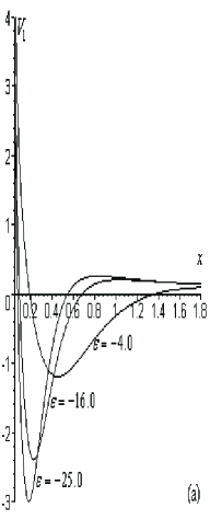
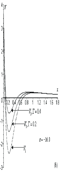
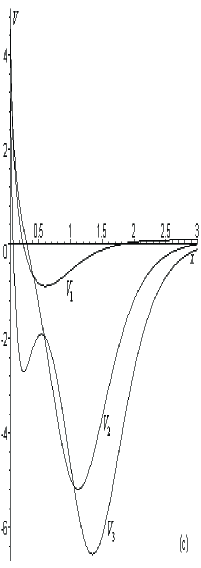
Figure 1: (a) Potentials $v_{1}(x)$ corresponding to one bound state created at different energies.  (b) Completely isospectral potentials with bound state energy ${\cal E}_{1}=-16.0$, dashed line corresponds to the initial potential $v_{1}$, solid lines correspond to its isospectral potentials. (c) Potentials $v_{n},~{}n=1,2,3$ having one, two and three bound states, respectively.

As an illustrative example we present the potentials $v_{1}$, obtained at the energy of transformation ${\cal E}_{1}=-4$, $v_{2}$ obtained at the energies ${\cal E}_{1}=-4,~{}{\cal E}_{2}=-16$ and $v_{3}$ calculated at the energies of transformation ${\cal E}_{1}=-4,~{}{\cal E}_{2}=-16,~{}{\cal E}_{3}=-25$. They are depicted in Fig.1c.

Now we are going to construct isospectral potentials. As an initial potential we take the potential $v_{1}$, obtained within the first-order intertwining (101). Using (95) and changing $v$ by $v_{1}$ from (101) and ${\cal U}_{1}$ by ${\cal U}$ from (103) after simplification we obtain a family of potentials with the same eigen-value and different values $\Gamma$

$$v_{3}(x)=\frac{1}{4x}-\frac{2x\kappa_{1}}{\cosh^{2}(\kappa_{1}~{}x)}-2x\frac{d}{dx}\ln\left[1+\Gamma\tanh\kappa_{1}~{}x\right]$$ (110)

The initial potential $v_{1}$ and its isospectral potentials (110) are presented in Fig.1b.

The 2-nd example. As the following example let us consider creation of new bound states for effective mass Schrödinger equation

$$-\left[\frac{d}{dx}\left(\frac{1}{m(x)}\right)\frac{d}{dx}\right]\phi(x)+v(x)\phi(x)={\cal E}~{}\phi(x)$$ (111)

that corresponds to the generalized equation (1) with $q(x)=1$. We choose the effective mass in the form $m(x)=\alpha^{2}/x^{2}$, the initial potential $v(x)=0$ and start with the equation

$$-\left[\frac{d}{dx}\left(\frac{1}{m(x)}\right)\frac{d}{dx}\right]\phi(x)={\cal E}~{}\phi(x).$$ (112)

The general solution of equation(112) can be written as

$$\phi(x)=\frac{\alpha}{\sqrt{x}}\left[c_{1}~{}\sin(\alpha\nu\ln(x))+c_{2}\cos(\alpha\nu\ln(x))\right],$$ (113)

where $c_{1},~{}c_{2}$ are free constants and $\nu^{2}=(-1+4\alpha^{2}k^{2})/4\alpha^{2}$. Recently in suz-shul we have constructed the potentials for effective mass Schrodinger equation (111) with creation of one and two bound states without investigation of potential forms. Here we would like to apply our technique to construction of double-well and even triple-well potentials with creation of two and three bound states, to generation of completely isospectral potentials and to investigation of the influence of position dependent mass on the form of constructed potentials.

Construction of completely isospectral potentials. As an initial potential we take the potential $v_{1}$, obtained in suz-shul within the $1$-st order intertwining

$$v_{1}=-\frac{2\gamma^{2}}{\cosh^{2}\left(\alpha\gamma\ln(x)\right)}.$$ (114)

It can be easily obtained from (56) at q(x)=1 with a particular solution of $\eta_{1}$ given as $\eta_{1}(x)=\sqrt{\frac{\alpha}{x}}~{}\cosh\left(\alpha\gamma_{1}\ln(x)\right)~{}.$ The solution at energy of transformation ${\cal E}_{1}=-\kappa_{1}^{2}$ is

$${\cal U}=\frac{\sqrt{m^{*}(x)}}{\eta_{1}(x)}=\frac{\sqrt{\alpha}}{\sqrt{x}\cosh\left(\alpha\gamma\ln(x)\right)}.$$ (115)

and corresponds to the bound state. Using (95) and replacing $v$ by $v_{1}$ from (114) and ${\cal U}_{1}$ by ${\cal U}$ from (115) after simplification we obtain two-parametric family of isospectral potentials

$$v_{3}=-\frac{2\gamma^{2}}{\cosh^{2}\left(\alpha\gamma\ln(x)\right)}-\frac{2x}{\alpha}\frac{d}{dx}\left[\frac{x}{\alpha}\frac{d}{dx}\ln P\right]~{},$$ (116)

where

$$P=1+\Gamma\int^{x}\frac{\alpha^{2}}{x^{2}\cosh^{2}\left(\alpha\gamma\ln(x)\right)}dx~{}.$$

All these potentials $v_{3}$ posses a single bound state each with the same energy ${\cal E}_{1}=-\kappa_{1}^{2}$ as the initial potential $v_{1}$, as well as the normalization constants including in $\Gamma$ can be chosen arbitrary. In Fig.2a we have plotted the initial potential calculated by the formula (114) and its strictly isospectral potentials, calculated by (116) at different $\Gamma$ .
Influence of distance between levels and effective mass on the form of potentials. By using second-order intertwining let us construct a potential with creation of two bound states. For this we define the auxiliary transformation functions as follows

$$\eta_{1}(x)=\sqrt{\frac{\alpha}{x}}~{}\cosh\left(\alpha\gamma_{1}\ln(x)\right),~{}~{}~{}\eta_{2}(x)=\sqrt{\frac{\alpha}{x}}\sinh\left(\alpha\gamma_{2}\ln(x)\right),$$ (117)

where $\gamma_{i}^{2}=-(1+4\alpha^{2}\kappa_{i}^{2})/4\alpha^{2},~{}~{}i=1,2$. We put $\kappa_{1}<\kappa_{2}$. The potential $v_{2}$, obtained within the second-order Darboux transformation, can be expressed from (106) with $q(x)=1$

$$v_{2}=v-\frac{2}{\sqrt{m}}\frac{d}{dx}\left[\frac{1}{W_{12}}~{}\frac{d}{dx}\frac{W_{12}}{\sqrt{m}}\right]-\frac{2}{\sqrt{m}}\frac{d^{2}}{dx^{2}}\frac{1}{\sqrt{m}}~{}.$$ (118)

This formula coincides with expression obtained in suz-shul for effective mass Schrödinger equation. For our choice of $m(x)$ the last term vanishes and the potential is written as

$$v_{2}=-\frac{2x}{\alpha}\frac{d}{dx}\left[\frac{x}{\alpha}~{}\frac{d}{dx}\ln{W_{12}}\right]~{},$$ (119)

where Wronskian is determined as

$$W_{12}=\frac{\alpha^{2}}{x^{2}}\Bigl{(}\gamma_{2}\cosh(\alpha\gamma_{2}\ln(x))\cosh(\alpha\gamma_{1}\ln(x))-\gamma_{1}\sinh(\alpha\gamma_{1}\ln x)\sinh(\alpha\gamma_{2}\ln(x))\Bigr{)}.$$

The potentials having two bound states are presented in Fig.2 b,c.

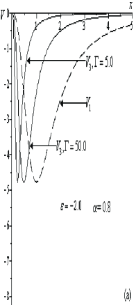
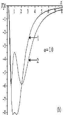
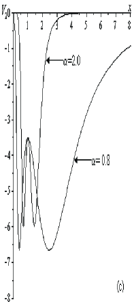
Figure 2: (a) Completely isospectral potentials with bound state energy ${\cal E}_{1}=-2.0$, dashed line corresponds to the initial potential $v_{1}$, solid lines correspond to isospectral partner potentials. (b) The change in form of potentials $v_{2}(x)$ with two bound states as the levels approach each other: $~{}1.\to{\cal E}_{1}=-2.0,~{}{\cal E}_{2}=-6.0,~{}2.\to{\cal E}_{1}=-2.0,~{}{\cal E}_{2}=-3.75$. (c) The influence of $m(x)$ on the behavior of transformed potentials $v_{2}(x)$ with two bound states ${\cal E}_{1}=-2.0,~{}{\cal E}_{2}=-3.75$.

The graphs in (Fig.2 b) depict the forms of constructed potentials in dependence from the distance between energy levels. One can see if the levels are close to each other, we construct asymmetric double well potentials (curves in Fig.2 2b) another, we construct asymmetric potentials (Fig.2 1b). Note, double well potentials have attracted some attention over the last years (see, e.g., Sukhatme ; Novaes ; Tralle ). Asymmetric double well potentials for the ordinary Schrödinger equation were investigated in Sukhatme with introducing a special parameter of asymmetry. In our case asymmetry in forms is a consequence of the position-dependent mass $m(x)$ that is singular at zero. The influence of $m(x)$ on the form of constructed potential $v(x)$ is demonstrated in Fig.2 c,b.

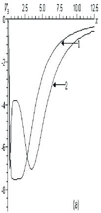
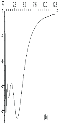
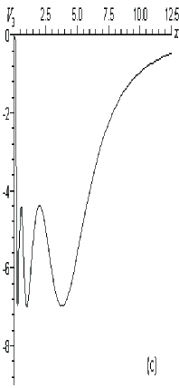
Figure 3: The change in form of potentials $V_{3}(x)$ with tree bound states as the levels come close to each other: $~{}(a)~{}1.\to{\cal E}_{1}=-1.0,~{}{\cal E}_{2}=-3.75,~{}{\cal E}_{3}=-6.25,~{}~{}2.\to{\cal E}_{1}=-1.0,~{}{\cal E}_{2}=-3.75,~{}{\cal E}_{3}=-5.0;$  $(b)~{}{\cal E}_{1}=-2.0,\break~{}{\cal E}_{2}=-4.75,~{}{\cal E}_{3}=-6.0;$  $(c)~{}~{}{\cal E}_{1}=-2.0,~{}{\cal E}_{2}=-3.75,~{}{\cal E}_{3}=-5.0$.

Our analysis shows that the larger $\alpha$, the shallow and narrow constructed potential (see Fig. 2 b, curve 2 and Fig. 2 c). Another words, increasing $m(x)$ leads to decreasing potential $v(x)$.

The next considered example illustrates the possibility to construct potentials having three bound states, for all that we can generate double well potentials and even triple well potentials. Employing the third-order Darboux transformations (79) with $q(x)=1$, the potential $v_{3}$ can be written as

$$v_{3}=-\frac{2x}{\alpha}\frac{d}{dx}\left[\frac{x}{\alpha}~{}\frac{d}{dx}\ln{W_{123}}\right]~{}.$$ (120)

The Wronskian $W_{1,2,3}$ is determined by the auxiliary functions $\eta_{1}(x),~{}\eta_{2}(x),~{}\eta_{3}(x)$, where $\eta_{1}(x)$, $\eta_{2}(x)$, is defined in (117) and $\eta_{3}$ is given as $\eta_{3}(x)=\sqrt{\frac{\alpha}{x}}~{}\cosh\left(\alpha\gamma_{3}\ln(x)\right).$ The potentials $v_{3}$ calculated by the formula (120) are plotted in Fig.3. As in the previous case with two bound states, the forms of constructed potentials depend on the space between energy levels. We can see if levels are sufficiently distant from one another, we construct simple asymmetric potentials presented in Fig.3 a (curve 1), if two levels out of three are close to each other, we construct asymmetric double well potentials (Fig.3 a, curve 2), if three levels are close to each other, we construct asymmetric triple well potentials (Fig.3 b, and Fig.3 c). As a final remark, let us note that different distances between levels give us different shapes of potentials. It can be very important for construction and investigation of quantum systems with needed spectral properties, e.g. in nanoelectronics Tralle .

Conclusion

By application of the intertwining operator technique to generalized Schrödinger equation with position dependent mass and with energy dependent potentials, Darboux transformations of an arbitrary order have been constructed. It has been shown that $n$th order Darboux transformation is equivalent to the resulting action of a chain of first-order Darboux transformations. Our generalized Darboux transformations comprises the position-dependent effective mass case and the case of linearly energy-dependent potentials, as well as the conventional case of Schrödinger equation. The integral Darboux transformation method has been elaborated for the generalized Schrödinger equation. An interrelation has been found between the differential and integral transformations. The integral Darboux transformations have been applied to generation of isospectral Hamiltonians differing by one and by two bound states from the spectrum of the initial one. It has been shown how to produce completely isospectral Hamiltonians to a given initial one. On concrete examples it has been demonstrated how to apply the Darboux transformation technique for modeling quantum well potentials with the given spectrum. Hamiltonians with different number of levels have been produced and the influence of the distance between levels on the shape of constructed potentials has been investigated, in particular, asymmetric double well and triple well potentials have been built. The influence of the position-dependent mass on the behaviour of constructed potentials has been studied, too.

References

- (1) E. Schrödinger, Proc.Roy.Irish. Acad., A. 46 (1940) p.9; A. 47, 53 (1941).
- (2) M.G. Darboux, Comptes Rendus Acad. Sci. Paris. 94, 1343 (1882); 94, 1456 (1882).
- (3) E. Witten, Nucl.Phys. B 185 (1981) 513; B 202, 253 (1982).
- (4) V.G. Bagrov, D.M. Gitman, Exact Solutions of Relativistic Wave Equations, (Kluwer Academic Publishers, Dordrecht/ Boston/ London) 1990, 323p.
- (5) K. Chadan, P. C. Sabatier, ”Inverse Problems in Quantum Scattering Theory”, 2nd edn (New York: Springer) 1989, 499p.
- (6) B.N. Zakhariev and A.A. Suzko, ”Direct and inverse problems, (Potentials in quantum scattering)”, (New York: Springer) 1990, 223p.
- (7) Junker G. ”Supersymmetric Method in Quantum and Statistical Physics”, (New York: Springer), 1996, 173p.
- (8) V.B. Matveev and M.A. Salle, Darboux transformations and solitons, (Springer, Berlin, 1991)
- (9) C. Gu, H. Hu and Z. Zhou, Darboux transformations in integrable systems, (Mathematical Physics Studies 26, Springer, Dordrecht, The Netherlands, 2005)
- (10) A.A. Andrianov, M.V. Ioffe, V. Spiridonov, Phys. Lett. A 174, 273 (1993); A.A. Andrianov, F. Cannata, J.Phys. A 37, 10297 (2004).
- (11) R.D. Amado, F. Cannata and J.P. Dedonder, Phys. Rev. Lett. 61, 2901 (1988); Phys. Rev. A38, 3797 (1988); Int. J. Mod. Phys. 5, 3401 (1990).
- (12) B.V. Rudyak, A.A. Suzko, B.N. Zakhariev, Physica Scripta, 29, 515 (1984)
- (13) A.A. Suzko, Physica Scripta, 31 (1985) 447; Physica Scripta, 34, 5 (1986);
- (14) A.A. Suzko, Sov. J. Nuclear Physics 55, 1359 (1992); Sov.J.Part. and Nucl. 24, No.4, 485 (1993); /in: /Quantum Inversion Theory and its Applications, Lect. Notes in Phys., vol. 427, Ed. H. Geramb, Springer, Berlin, 1993, pp. 67-106.
- (15) I. M. Gel’fand, B. M. Levitan, Izv.Akad.Nauk. SSR ser.Math. 15, p. 309-360 (1951).
- (16) Z. S. Agranovich, V. A. Marchenko, Inversion Problem of Scattering Theory (Gordon and Breach, New York) 1963.
- (17) B.M. Levitan, Inverse Sturm-Liouville problems, Nauka, Moscow, 1984.
- (18) V.E. Zakharov, A.B. Shabat, Funct. Anal. Appl. 8, 226 (1974); ibid. 13, 166 (1979).
- (19) B. Pavlov, The Theory of Extensions and explicitly solvable models, (In Russian) Uspekhi Mat. Nauk, 42, 99 (1987).
- (20) A.A. Suzko, G. Giorgadze, Physics of Atomic Nuclei, 70, 604 (2007); A.A. Suzko, I. Tralle, Acta Physica Polonioca B, 39, No.3, p. 1001-1023 (2008).
- (21) H. Feshbach, Ann.Phys.(N.Y.) 5, 357 (1958).
- (22) P.Fröbrich and R. Lipperhide, Theory of Nuclear Reaction (Clarendon, Oxford, 1996).
- (23) P.Ring and P.Schuck, The Nuclear Many Body Problem, Springer, New York, 1980 p.211
-
(24)
V.V. Babikov, Method of Phase function
in Quntum Mechanics, Nauka, Moscow, 1976;
S.I. Vinitsky et.al., Physics of Atomic Nuclei, 64, 27 (2001);
M.I. Jaghoub, Phys. Rev.A 74, 032702 (2006). - (25) F. Arias de Saavedra et.al, Phys. Rev. B 50, 4248 (1994).
- (26) R.A. Morrow and K.R. Brownstein, Phys. Rev. B 30, 678 (1984).
- (27) G.T. Einevoll, P.C. Hemmer and J.Thomesn, Phys. Rev. B 42, 3485 (1990).
- (28) A.R. Plastino et al., Phys. Rev. A 60, 4318 (1999).
- (29) V. Milanović, Z. Iconić, J.Phys. A: Math.Gen. 32, 7001 (1999).
- (30) B. Roy and P. Roy, J.Phys. A 35, 3961 (2002).
- (31) R.Koç and M.Koca, J.Phys. A 36, 8105 (2003).
- (32) C. Quesne, Annals of Physics 321, Issue 5, 1221 (2006).
- (33) A.A. Suzko and A. Schulze-Halberg, J.Phys. A; Math.Gen. 42, 295203 (2009).
- (34) A.A. Suzko and A. Schulze-Halberg, Phys.Lett. A, 372, 5865 (2008).
- (35) Bikashkali Midya, B. Roy, R.Roychoudhury, J.Math.Phys. 51, 022109 (2010).
- (36) A.A. Suzko, A. Schulze-Halberg, E.P. Velicheva, Physics of Atomic Nuclei, 72, 858 (2009).
- (37) K. Goser, P. Glösekötter, J. Dienstuhl, Nanoelectronics and Nanosystems. From Transistors to Molecular and Quantum Devices. Springer-Verlag, Berlin, 2004.
- (38) Special issue of Physica E: Low-dimensional Systems and Nanostructures, 14, No.1/2, 2002
- (39) G. Bastard, Wave Mechanics applied to semiconductor heterostructure(Les Editions de Physique, Les Ulis, France, 1988).
-
(40)
F.Cooper, A.Khare, U.Sukhatme, Physics Reports, 251,
p. 267-385 (1995);
Wai-Yee Keung, Eve Kovacs, U.P. Sukhatme, Phys. Rev. Lett. 60, 41 (1988);
A. Gangopadhyaya, P.K. Panigrahi, U. P. Sukhatme, Phys. Rev. A, 47, 2720 (1993). - (41) M. Novaes, M.A.M. Aguiar, J.E.M. Hornos, J.Phys. A; Math.Gen. 36, 5773 (2003).
- (42) K. Majchrowski, W.Paśko, I. Tralle, Phys. Lett.A, 373, 2959. (2009)
- (43) L.D. Faddeev Usp. Mat. Nauk 14, 57 (1959).