Quantum Phase Estimation with Arbitrary Constant-precision Phase Shift Operators

Abstract

While Quantum phase estimation (QPE) is at the core of many quantum algorithms known to date, its physical implementation (algorithms based on quantum Fourier transform (QFT) ) is highly constrained by the requirement of high-precision controlled phase shift operators, which remain difficult to realize. In this paper, we introduce an alternative approach to approximately implement QPE with arbitrary constant-precision controlled phase shift operators.

The new quantum algorithm bridges the gap between QPE algorithms based on QFT and Kitaev’s original approach. For approximating the eigenphase precise to the nth bit, Kitaev’s original approach does not require any controlled phase shift operator. In contrast, QPE algorithms based on QFT or approximate QFT require controlled phase shift operators with precision of at least Pi/2n. The new approach fills the gap and requires only arbitrary constant-precision controlled phase shift operators. From a physical implementation viewpoint, the new algorithm outperforms Kitaev’s approach.

1 Introduction

Quantum Phase Estimation (QPE) plays a core role in many quantum algorithms [4, 10, 11, 13, 14]. Some interesting algebraic and theoretic problems can be addressed by QPE, such as prime factorization [10], discrete-log finding [11], and order finding.

Problem.

[Phase Estimation] Let $U$ be a unitary matrix with eigenvalue $e^{2\pi i\varphi}$ and corresponding eigenvector $|u\rangle$. Assume only a single copy of $\left|{u}\right\rangle$ is available, the goal is to find $\widetilde{\varphi}$ such that

$$\Pr(|\widetilde{\varphi}-\varphi|<\frac{1}{2^{n}})>1-c,$$ (1)

where $c$ is a constant less than $\frac{1}{2}$.

In this paper we investigate a more general approach for the QPE algorithm. This approach completes the transition from Kitaev’s original approach that requires no controlled phase shift operators, to QPE with approximate quantum Fourier transform (AQFT). The standard QPE algorithm utilizes the complete version of the inverse QFT. The disadvantage of the standard phase estimation algorithm is the high degree of phase shift operators required. Since implementing exponentially small phase shift operators is costly or physically not feasible, we need an alternative way to use lower precision operators. This was the motivation for AQFT being introduced — for lowering the cost of implementation while preserving high success probability.

In AQFT the number of required phase shift operators drops significantly with the cost of lower success probability. Such compromise demands repeating the process extra times to achieve the final result. The QPE algorithm has a success probability of at least $\frac{8}{\pi^{2}}$ [6]. Phase estimation using AQFT instead, with phase shift operators up to degree $m$ where $m>\log_{2}(n)+2$, has success probability at least $\frac{4}{\pi^{2}}-\frac{1}{4n}$ [1, 2].

On the other hand, Kitaev’s original approach requires only the first phase shift operator (as a single qubit gate not controlled). Comparing the existing methods, there is a gap between Kitaev’s original approach and QPE with AQFT in terms of the degree of phase shift operators needed. In this paper our goal is to fill this gap and introduce a more general phase estimation algorithm such that it is possible to realize a phase estimation algorithm with any degree of phase shift operators in hand. In physical implementation of the phase estimation algorithm, the depth of the circuit should be small to avoid decoherence. Also, higher degree phase shift operators are costly to implement and in many cases it is not physically feasible.

In this paper, we assume only one copy of the eigenvector $\left|{u}\right\rangle$ is available. This implies a restriction on the use of controlled-$U$ gates that all controlled-$U$ gates should be applied on one register. Thus, the entire process is a single circuit that can not be divided into parallel processes. Due to results by Griffiths and Niu, who introduced semi classical quantum Fourier transform [3], quantum circuits implementing different approaches discussed in this paper would require the same number of qubits.

The structure of this paper is organized as follows. In Sec. 2 we give a brief overview on existing approaches, such as Kitaev’s original algorithm and standard phase estimation algorithm based on QFT and AQFT. In Sec. 3 we introduce our new approach and discuss the requirements to achieve the same performance output (success probability) as the methods above. Finally, we make our conclusion and compare with other methods.

2 Quantum phase estimation algorithms

2.1 Kitaev’s original approach

Kitaev’s original approach is one of the first quantum algorithms for estimating the phase of a unitary matrix [8]. Let $U$ be a unitary matrix with eigenvalue $e^{2\pi i\varphi}$ and corresponding eigenvector $\left|{u}\right\rangle$ such that

$$U\left|{u}\right\rangle=e^{2\pi i\varphi}\left|{u}\right\rangle.$$ (2)

In this approach, a series of Hadamard tests are performed. In each test the phase $2^{k-1}\varphi$ ($1\leq k\leq n$) will be computed up to precision $1/16$. Assume an $n$-bit approximation is desired. Starting from $k=n$, in each step the $k$th bit position is determined consistently from the results of previous steps.

For the $k$th bit position, we perform the Hadamard test depicted in Figure 1, where the gate $K=I_{2}$. Denote $\varphi_{k}=2^{k-1}\varphi$, the probability of the post measurement state is

$$\Pr(0|k)=\frac{1+\cos(2\pi\varphi_{k})}{2},\quad\Pr(1|k)=\frac{1-\cos(2\pi\varphi_{k})}{2}.$$ (3)

In order to recover $\varphi_{k}$, we obtain more precise estimates with higher probabilities by iterating the process. But, this does not allow us to distinguish between $\varphi_{k}$ and $-\varphi_{k}$. This can be solved by the same Hadamard test in Figure 1, but instead we use the gate

$$K=\left({\begin{array}[]{cc}1&0\\ 0&i\\ \end{array}}\right).$$ (4)

The probabilities of the post-measurement states based on the modified Hadamard test become

Figure 1: Hadamard test with extra phase shift operator.

$$\Pr(0|k)=\frac{1-\sin(2\pi\varphi_{k})}{2},\quad\Pr(1|k)=\frac{1+\sin(2\pi\varphi_{k})}{2}.$$ (5)

Hence, we have enough information to recover $\varphi_{k}$ from the estimates of the probabilities.

In Kitaev’s original approach, after performing the Hadamard tests, some classical post processing is also necessary. Suppose $\varphi=0.x_{1}x_{2}\ldots x_{n}$ is an exact $n$-bit. If we are able to determine the values of $\varphi$, $2\varphi,\ldots,$ $2^{n-1}\varphi$ with some constant-precision ($1/16$ to be exact), then we can determine $\varphi$ with precision $1/2^{n}$ efficiently [7, 8].

Starting with $\varphi_{n}$ we increase the precision of the estimated fraction as we proceed toward $\varphi_{1}$. The approximated values of $\varphi_{k}\,(k=n,\ldots,1)$ will allow us to make the right choices.

For $k=1,\ldots,n$ the value of $\varphi_{k}$ is replaced by $\beta_{k}$, where $\beta_{k}$ is the closest number chosen from the set $\{\frac{0}{8},\frac{1}{8},\frac{2}{8},\frac{3}{8},\frac{4}{8},\frac{5}{8},\frac{6}{8},\frac{7}{8}\}$ such that

$$|\varphi_{k}-\beta_{k}|_{\text{mod 1}}<\frac{1}{8}.$$ (6)

The result follows by a simple iteration. Let $\beta_{n}=\overline{0.x_{n}x_{n+1}x_{n+2}}$ and proceed by the following iteration:

$$x_{k}=\left\{\begin{array}[]{l l}0&\quad\mbox{if $\overline{0.0x_{k+1}x_{k+2}}-\beta_{k}|_{\text{mod 1}}<1/4$ }\\ 1&\quad\mbox{if $\overline{0.1x_{k+1}x_{k+2}}-\beta_{k}|_{\text{mod 1}}<1/4$}\\ \end{array}\right.$$ (7)

for $k=n-1,\ldots,1$. By using simple induction, the result satisfies the following inequality:

$$|\overline{0.x_{1}x_{2}\ldots x_{n+2}}-\varphi|_{\text{mod 1}}<2^{-(n+2)}.$$ (8)

In Eq. 6, we do not have the exact value of $\varphi_{k}$. So, we have to estimate this value and use the estimate to find $\beta_{k}$. Let $\widetilde{\varphi_{k}}$ be the estimated value and

$$\epsilon=|\widetilde{\varphi_{k}}-\varphi_{k}|_{\text{mod 1}}$$ (9)

be the estimation error. Now we use the estimate to find the closest $\beta_{k}$. Since we know the exact binary representation of the estimate $\widetilde{\varphi_{k}}$, we can choose $\beta_{k}$ such that

$$|\widetilde{\varphi_{k}}-\beta_{k}|_{\text{mod 1}}\leq\frac{1}{16}.$$ (10)

By the triangle inequality we have,

$$|\varphi_{k}-\beta_{k}|_{\text{mod 1}}\leq|\widetilde{\varphi_{k}}-\varphi_{k}|_{\text{mod 1}}+|\widetilde{\varphi_{k}}-\beta_{k}|_{\text{mod 1}}\leq\epsilon+\frac{1}{16}.$$ (11)

To satisfy Eq. 6, we need to have $\epsilon<1/16$, which implies

$$|\widetilde{\varphi_{k}}-\varphi_{k}|_{\text{mod 1}}<\frac{1}{16}.$$ (12)

Therefore, it is required for the phase to be estimated with precision $1/16$ at each stage.

In the first Hadamard test (Eq. 3), in order to estimate $\Pr(1|k)$ an iteration of Hadamard tests should be applied to obtain the required precision of $1/16$ for $\varphi_{k}$. This is done by counting the number of states $\left|{1}\right\rangle$ in the post measurement state and dividing that number by the total number of iterations performed.

The Hadamard test outputs $\left|{0}\right\rangle$ or $\left|{1}\right\rangle$ with a fixed probability. We can model an iteration of Hadamard tests as Bernoulli trials with success probability (obtaining $\left|{1}\right\rangle$) being $p_{k}$. The best estimate for the probability of obtaining the post measurement state $\left|{1}\right\rangle$ with $t$ samples is

$$\widetilde{p_{k}}=\frac{h}{t},$$ (13)

where $h$ is the number of ones in $t$ trials. This can be proved by Maximum Likelihood Estimation (MLE) methods [5].

In order to find $\sin(2\pi\varphi_{k})$ and $\cos(2\pi\varphi_{k})$, we can use estimates of probabilities in Eq. 3 and EQ. 5. Let $s_{k}$ be the estimate of $\sin(2\pi\varphi_{k})$ and $t_{k}$ the estimate of $\cos(2\pi\varphi_{k})$. It is clear that if

$$|\widetilde{p_{k}}-p_{k}|<\epsilon_{0},$$ (14)

then

$$|s_{k}-\sin(2\pi\varphi_{k})|<2\epsilon_{0},\quad|t_{k}-\cos(2\pi\varphi_{k})|<2\epsilon_{0}.$$ (15)

Since the inverse tangent function is more robust to error than the inverse sine or cosine functions, we use

$$\widetilde{\varphi_{k}}=\frac{1}{2\pi}\arctan\left(\frac{s_{k}}{t_{k}}\right)$$ (16)

as the estimation of $\varphi_{k}$. By Eq. 12 we should have

$$\left|\varphi_{k}-\frac{1}{2\pi}\arctan\left(\frac{s_{k}}{t_{k}}\right)\right|_{\text{mod 1}}<\frac{1}{16}.$$ (17)

The inverse tangent function can not distinguish between the two values $\varphi_{k}$ and $\varphi_{k}\pm 1/2$. However, because we find estimates of the sine and cosine functions as well, it is easy to determine the correct value. The inverse tangent function is most susceptible to error when $\varphi_{k}$ is in the neighborhood of zero and the reason is that the derivative is maximized at zero. Thus, if

$$|s_{k}-\sin(2\pi\varphi_{k})|=\epsilon_{1}\quad\text{and}\quad|t_{k}-\cos(2\pi\varphi_{k})|=\epsilon_{2},$$ (18)

considering the case where $\varphi_{k}=0$, then we have

$$\frac{1}{2\pi}\left|\arctan\left(\frac{\epsilon_{1}}{1\pm\epsilon_{2}}\right)\right|<\frac{1}{16}.$$ (19)

By simplifying the above inequality, we have

$$\left|\frac{\epsilon_{1}}{1\pm\epsilon_{2}}\right|<\tan(\frac{\pi}{8}).$$ (20)

With the following upper bounds for $\epsilon_{1}$ and $\epsilon_{2}$, the inequality above is always satisfied when

$$|\epsilon_{1}|<1-\frac{1}{\sqrt{2}}\quad\text{and}\quad|\epsilon_{2}|<1-\frac{1}{\sqrt{2}}.$$ (21)

Therefore, in order to estimate the phase $\varphi_{k}$ with precision $1/16$, the probabilities in Eq. 3 and Eq. 5 should be estimated with error at most $(2-\sqrt{2})/4$ which is approximately 0.1464. In other words, it is necessary to find the estimate of $\Pr(1|k)$ such that

$$\left|\Pr(1|k)-\frac{h}{t}\right|<\frac{2-\sqrt{2}}{4}\approx 0.1464.$$ (22)

There are different ways we can guarantee an error bound with constant probability. The first method, used in [8], is based on the Chernoff bound. Let $X_{1},\ldots,X_{m}$ be Bernoulli random variables, by Chernoff’s bound we have

$$\mathrm{Pr}\left(\left|\frac{1}{m}\sum_{i=0}^{m}X_{i}-p_{k}\right|\geq\delta\right)\leq 2e^{-2\delta^{2}m},$$ (23)

where in our case the estimate is $\widetilde{p_{k}}=\frac{1}{m}\sum_{i=0}^{m}X_{i}$. Since we need an accuracy up to $0.1464$, we get

$$\mathrm{Pr}\left(|\widetilde{p_{k}}-p_{k}|>0.1464\right)<2e^{-(0.0429)m}.$$ (24)

In order to obtain

$$\mathrm{Pr}\left(\left|\widetilde{p_{k}}-p_{k}\right|<0.1464\right)>1-\frac{\varepsilon}{2},$$ (25)

a minimum of $m_{1}$ trials is sufficient when

$$m_{1} \approx 24\ln\frac{4}{\varepsilon}$$ (26)

$$\approx 33+24\ln\frac{1}{\varepsilon}$$

This is the number of trials for each Hadamard test, as we have two Hadamard tests at each stage. Therefore, in order to have

$$\mathrm{Pr}\left(|\widetilde{\varphi_{k}}-\varphi_{k}|<\frac{1}{16}\right)>1-\varepsilon.$$ (27)

we require a minimum of

$$m = 2m_{1}$$ (28)

$$\approx 47\ln\frac{4}{\varepsilon}$$

$$\approx 66+47\ln\frac{1}{\varepsilon}$$

many trials.

In the analysis above, we used the Chernoff bound, which is not a tight bound. If we want to obtain the result with a high probability, we need to apply a large number of Hadamard tests. In this case, we can use an alternative method to analyze the process by employing methods of statistics [12].

Iterations of Hadamard tests have a Binomial distribution which can be approximated by a normal distribution. This is a good approximation when $p$ is close to $1/2$ or $mp>10$ and $m(1-p)>10$, where $m$ is the number of iterations and $p$ the success probability. In other words, if we see $10$ successes and $10$ fails in our process, we can use this approximation to obtain a better bound.

In Kitaev’s algorithm each Hadamard test has to be repeated a sufficient number of times to achieve the required accuracy with high probability. Because only one copy of $\left|{u}\right\rangle$ is available, all controlled-$U$ gates have to be applied to one register. Therefore, all the Hadamard tests have to be performed in sequence, instead of parallel, during one run of the circuit. A good example for this case is the order finding algorithm. We refer the reader to [9] for more details.

In Kitaev’s approach, there are $n$ different Hadamard tests that should be performed. Thus, if the probability of error in each Hadamard test is $\varepsilon_{0}$, by applying the union bound, the error probability of the entire process is $\varepsilon=n\varepsilon_{0}$. Therefore, in order to obtain

$$\Pr(|\varphi-\widetilde{\varphi}|<\frac{1}{2^{n}})>1-\varepsilon,$$ (29)

for approximating each bit we need $m$ trials where

$$m=47\ln\frac{4n}{\varepsilon}.$$ (30)

Since, all of these trials have to be done in one circuit, the circuit consists of $mn$ Hadamard tests. Therefore the circuit involves $mn$ controlled-$U^{2^{k}}$ operations. As a result, if a constant success probability is desired, the depth of the circuit will be $O(n\log n)$.

2.2 Approach based on QFT

One of the standard methods to approximate the phase of a unitary matrix is QPE based on QFT. The structure of this method is depicted at Figure  2. The QPE algorithm requires two registers and contains two stages. If an $n$-bit approximation of the phase $\varphi$ is desired, then the first register is prepared as a composition of $n$ qubits initialized in the state $|0\rangle$. The second register is initially prepared in the state $\left|{u}\right\rangle$. The first stage prepares a uniform superposition over all possible states and then applies controlled-$U^{2^{k}}$ operations. Consequently, the state will become

$$\frac{1}{2^{n/2}}\sum_{k=0}^{2^{n}-1}e^{2\pi i\varphi k}|k\rangle.$$ (31)

The second stage in the QPE algorithm is the QFT^† operation.

Figure 2: Standard Quantum Phase Estimation.

There are different ways to interpret the inverse Fourier transform. In the QPE algorithm, the post-measurement state of each qubit in the first register represents a bit in the final approximated binary fraction of the phase. Therefore, we can consider computing each bit as a step. The inverse Fourier transform can be interpreted such that at each step (starting from the least significant bit), using the information from previous steps, it transforms the state

$$\frac{1}{\sqrt{2}}(\left|{0}\right\rangle+e^{2\pi i2^{k}\varphi}\left|{1}\right\rangle)$$ (32)

to get closer to one of the states

$$\frac{1}{\sqrt{2}}(\left|{0}\right\rangle+e^{2\pi i0.0}\left|{1}\right\rangle) = \frac{1}{\sqrt{2}}(\left|{0}\right\rangle+\left|{1}\right\rangle)$$

or

$$\frac{1}{\sqrt{2}}(\left|{0}\right\rangle+e^{2\pi i0.1}\left|{1}\right\rangle) = \frac{1}{\sqrt{2}}(\left|{0}\right\rangle-\left|{1}\right\rangle).$$ (33)

Assume we are at step $k$ in the first stage. By applying controlled-$U^{2^{k}}$ operators due to phase kick back, we obtain the state

$$\frac{\left|{0}\right\rangle+e^{2\pi i0.x_{k+1}x_{k+2}\ldots x_{n}}\left|{1}\right\rangle}{\sqrt{2}}.$$ (34)

Shown in Figure  3, each step (dashed-line box) uses the result of previous steps, where phase shift operators are defined as

$$R_{k}\equiv\left[{\begin{array}[]{cc}1&0\\ 0&e^{2\pi i/2^{k}}\\ \end{array}}\right]$$ (35)

for $2\leq k\leq n$.

Figure 3: 3-qubit inverse QFT where $1\leq i\leq 3$, $|y_{i}\rangle=\frac{1}{\sqrt{2}}(\left|0\right>+e^{2\pi i(0.x_{i}\ldots x_{3})}\left|1\right>$).

By using the previously determined bits $x_{k+2},\ldots,x_{n}$ and the action of corresponding controlled phase shift operators (as depicted in Figure 3) the state in Eq. 34 becomes

$$\frac{\left|{0}\right\rangle+e^{2\pi i0.x_{k+1}0\ldots 0}\left|{1}\right\rangle}{\sqrt{2}}=\frac{\left|{0}\right\rangle+(-1)^{x_{k+1}}\left|{1}\right\rangle}{\sqrt{2}}.$$ (36)

Thus, by applying a Hadamard gate to the state above we obtain $\left|{x_{k+1}}\right\rangle$. Therefore, we can consider the inverse Fourier transform as a series of Hadamard tests.

If $\varphi$ has an exact $n$-bit binary representation the success probability at each step is $1$. While, in the case that $\varphi$ cannot be exactly expressed in $n$-bit binary fraction, the success probability $P$ of the post-measurement state, at step $k$, is

$$P=\cos^{2}(\pi\theta)\quad\text{for}\quad|\theta|<\frac{1}{2^{k+1}}$$ (37)

Detailed analysis obtaining similar probabilities are given in Sec. 3.

Therefore, the success probability increases as we proceed. The following theorem gives us the success probability of the QFT algorithm.

Theorem 1 ([6]).

If $\frac{x}{2^{n}}\leq\varphi\leq\frac{x+1}{2^{n}}$, then the phase estimation algorithm returns one of $x$ or $x+1$ with probability at least $\frac{8}{\pi^{2}}$.

2.3 Approach based on AQFT

Figure 4: Quantum circuit for AQFT.

AQFT was first introduced by Barenco, et al [1]. It has the advantage in algorithms that involve periodicity estimation. Its structure is similar to regular QFT but differs by eliminating higher precision phase shift operators. The circuit of AQFT is shown in Figure 4. At the RHS of the circuit, for $n-m<i\leq n$

$$\left|{y_{i}}\right\rangle=\frac{1}{\sqrt{2}}(\left|0\right>+e^{2\pi i(0.x_{i}\ldots x_{n})}\left|1\right>)$$ (38)

and for $1<i\leq n-m$,

$$\left|{y_{i}}\right\rangle=\frac{1}{\sqrt{2}}(\left|0\right>+e^{2\pi i(0.x_{i}\ldots x_{i+m-1})}\left|1\right>).$$ (39)

Let $0.x_{1}x_{2}\ldots x_{n}$ be the binary representation of eigenphase $\varphi$. For estimating each $x_{p}$, where $1\leq p\leq n$, AQFT_m requires at most $m$ phase shift operations. Here $m$ is defined as the degree of the AQFT_m.

Therefore, phase shift operations in AQFT_m requires precision up to $e^{2\pi i/2^{m}}$. The probability $P$ of gaining an accurate output using AQFT_m, when $m\geq\log_{2}n+2$, is at least [1]

$$P\geq\frac{8}{\pi^{2}}(\sin^{2}(\frac{\pi}{4}\frac{m}{n})).$$ (40)

The accuracy of AQFT_m approaches the lower bound for the accuracy of the full QFT, which is $\frac{8}{\pi^{2}}$. A better lower bound is also achieved by Cheung in [2]

$$P\geq\frac{4}{\pi^{2}}-\frac{1}{4n}.$$ (41)

Moreover, this indicates the logarithmic-depth AQFT provides an alternative approach to replace the regular QFT in many quantum algorithms. The total number of the phase shift operator invocations in AQFT_m is $O(n\log_{2}n)$, instead of $O(n^{2})$ in the QFT. The phase shift operator precision requirement is only up to $e^{2\pi i/4n}$, instead of $e^{2\pi i/2^{n}}$.

By using the AQFT instead of the QFT we trade off smaller success probability with smaller degrees of phase shift operators and a shorter circuit.

3 New approach with constant degree phase shift operators

In this section we introduce our new approach for QPE. Our approach draws a trade-off between the highest degree of phase shift operators being used and the depth of the circuit. As a result, when smaller degrees of phase shift operators are used, the depth of the circuit increases and vice versa.

As pointed out in Sec. 2.2, by using information of previous qubits, the full-fledged inverse QFT transforms the phase such that the phase of the corresponding qubit gets closer to one of the states $\left|{+}\right\rangle$ or $\left|{-}\right\rangle$. For our approach, we first consider the case where only the controlled phase shifts operators $R_{2}$ and $R_{3}$ are used (Eq. 35). In this case, we only use the information of the two previous qubits (see Figure 5). In such a setting, we show that it is possible to perform the QPE algorithm with arbitrary success probability.

Figure 5: QPE with only two controlled phase shift operations.

The first stage of our algorithm is similar to the first stage of QPE based on QFT. Assume the phase is $\varphi=0.x_{1}x_{2}x_{3}\ldots$ with an infinite binary representation. At step $k$, the phase after the action of the controlled gate $U^{2^{k}}$ is $2^{k}\varphi=0.x_{k+1}x_{k+2}\ldots$ and the corresponding state is

$$\left|{\psi_{k}}\right\rangle=\frac{1}{\sqrt{2}}(\left|{0}\right\rangle+e^{2\pi i2^{k}\varphi}\left|{1}\right\rangle).$$ (42)

By applying controlled phase shift operators $R_{2}$ (controlled by the $(k-1)$th qubit) and $R_{3}$ (controlled by the $(k-2)$th qubit) to the state above, we obtain

$$\left|{\widetilde{\psi_{k}}}\right\rangle=\frac{1}{\sqrt{2}}(\left|{0}\right\rangle+e^{2\pi i\widetilde{\varphi}}\left|{1}\right\rangle),$$ (43)

where

$$\widetilde{\varphi}=0.x_{k+1}00x_{k+4}\ldots.$$ (44)

It is easy to see that

$$|\widetilde{\varphi}-0.x_{k+1}|<\frac{1}{8}.$$ (45)

Hence, we can express

$$\widetilde{\varphi}=0.x_{k+1}+\theta$$ (46)

where $|\theta|<\frac{1}{8}$. Therefore, the state $\left|{\widetilde{\psi_{k}}}\right\rangle$ can be rewritten as

$$\left|{\widetilde{\psi_{k}}}\right\rangle=\frac{1}{\sqrt{2}}(\left|{0}\right\rangle+e^{2\pi i(0.x_{k+1}+\theta)}\left|{1}\right\rangle).$$ (47)

In order to approximate the phase $\varphi$ at this stage ($k$th step), we need to find the value of $x_{k+1}$ by measuring the $k$th qubit. In this regard, we first apply a Hadamard gate before the measurement to the state $\left|{\widetilde{\psi_{k}}}\right\rangle$. The post-measurement state will determine the value of $x_{k+1}$ correctly with high probability. The post measurement probabilities of achieving $\left|{0}\right\rangle$ or $\left|{1}\right\rangle$ in the case where $x_{k+1}=0$ is

$$\Pr(0|k) = \cos^{2}(\pi\theta)$$

$$\Pr(1|k) = \sin^{2}(\pi\theta).$$ (48)

Therefore,

$$\Pr(0|k) \geq \cos^{2}(\frac{\pi}{8})\approx 0.85$$

$$\Pr(1|k) \leq \sin^{2}(\frac{\pi}{8})\approx 0.15$$ (49)

In the case where $x_{k+1}=1$, the success probability is similar.

By iterating this process a sufficient number of times and then letting the majority decide, we can achieve any desired accuracy. The analysis is similar to Sec. 2.1. In this case, all we require is to find the majority. Therefore, by a simple application of the Chernoff’s bound

$$\mathrm{Pr}\left(\frac{1}{m}\sum_{i=0}^{m}X_{i}\leq\frac{1}{2}\right)\leq e^{-2m(p-\frac{1}{2})^{2}},$$ (50)

where in this case $p=\cos^{2}(\pi/8)$. It is easy to see that if a success probability of $1-\varepsilon$ is required, then we need at least

$$m=4\ln(\frac{1}{\varepsilon})$$ (51)

many trials for approximating each bit.

By comparing Eq. 30 and Eq. 51 (Table 1), we see that while preserving the success probability, our new algorithm differs by a constant and scales about 12 times better than Kitaev’s original approach in terms of the number of Hadamard tests required (Figure 6). In physical implementations this is very important, especially in the case where only one copy of the eigenvector $\left|{u}\right\rangle$ is available and all Hadamard tests should be performed during one run of the circuit.

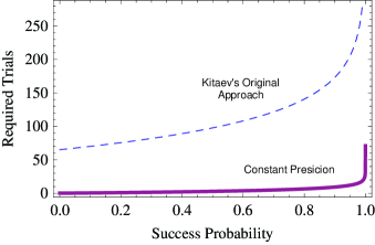
Figure 6: Required trails for estimating each bit in Kitaev’s original approach and our new approach.

In the algorithm introduced above, only phase shift operators $R_{2}$ and $R_{3}$ are used. When higher phase shift operators are used in our algorithm, the success probability of each Hadamard test will increase. As a result, fewer trials are required in order to achieve similar success probabilities. As pointed out in Sec. 2.3, the QPE based on AQFT requires phase shift operators of degree at least $2+\log n$. With this precision of phase shift operators in hand, the success probability at each step would be high enough such that there is no need to iterate each step. In such scenario, one trial is sufficient to achieve an overall success probability of a constant.

Success	Kitaev’s	Constant
Probability	Original Approach	Precision
0.50000	98	3
0.68269	120	5
0.95450	211	13
0.99730	344	24
0.99993	515	39

Table 1: Required trials for estimating each bit by using Chernoff’s bound.

Recall the phase estimation problem stated in the introduction. If a constant success probability greater than $\frac{1}{2}$ is required, the depth of the circuit for all the methods mentioned in this paper (except the QPE based on full fledged QFT, which is $O(n^{2})$), would be $O(n\log n)$ (assuming the cost of implementing the controlled-$U^{2^{k}}$ gates are all the same). This means the depth of the circuits differ only by a constant. However, the disadvantage of Kitaev’s original approach to our new approach is the large number of Hadamard tests required for each bit in the approximated fraction.

Therefore, the new method introduced in this paper provides the flexibility of using any available degree of controlled phase shift operators while preserving the success probability and the length of the circuit up to a constant.

4 Acknowledgments

We would like to thank Pawel Wocjan for useful discussions and Stephen Fulwider for helpful comments. H. A. and C. C. gratefully acknowledge the support of NSF grants CCF-0726771 and CCF-0746600.

References

- [1] A. Barenco, A. Ekert, K. Suominen and P. Törmä, Approximate Quantum Fourier Transform and Decoherence, vol. 54, issue 1, pp. 139 - 146, Phys. Rev. A, 1996
- [2] D. Cheung, Improved Bounds for the Approximate QFT, arXiv: abs/quant-ph/0403071, 2004.
- [3] R. B. Griffiths and C. Niu, Semiclassical Fourier Transform for Quantum Computation, Phys. Rev. Lett. 76, 3228 3231 (1996).
- [4] S. Hallgren, Polynomial-time Quantum Algorithms for Pell’s Equation and the Principal Ideal Problem. In Proceedings of the 34th ACM Symposium on Theory of Computing, 2002.
- [5] J. W. Harris and H. Stocker, Maximum Likelihood Method. Handbook of Mathematics and Computational Science. New York, Springer-Verlag, p. 824, (1998).
- [6] P. Kaye, R. Laflamme and M. Mosca, An Introduction to Quantum Computing, Oxford University Press, 2007.
- [7] A. Kitaev, Quantum Measurements and the Abelian Stabilizer Problem. Technical Report, arXiv:quant-ph/9511026, 1995.
- [8] A. Kitaev, A. Shen and M. Vyalyi, Classical and Quantum Computation, vol. 47, Graduate Studies in Mathematics, American Mathematical Society, 2002.
- [9] M. Nielsen and I. Chuang, Quantum Computation and Quantum Information, Cambridge University Press, 2000.
- [10] P. Shor, Algorithms for Quantum Computation: Discrete Logarithms and Factoring. Proceedings of FOCS, pg. 124-134, 1994.
- [11] P. Shor, Polynomial-time Algorithms for Prime Factorization and Discrete Logarithms on a Quantum Computer. SIAM Journal on Computing, 26(5):1484-1509, 2005.
- [12] D. Sivia: Data Analysis, a Bayesian Tutorial. Oxford University Press (1996).
- [13] M. Szegedy, Quantum Speed-up of Markov Chain Based Algorithms, Proc. of 45th Annual IEEE Symposium on Foundations of Computer Science, pp. 32–41, 2004.
- [14] P. Wocjan, C. Chiang, D. Nagaj and A. Abeyesinghe, A Quantum Algorithm for Approximating Partition Functions, Physical Review A, vol. 80, pp. 022340, 2009 .