Staggered chiral random matrix theory

Abstract

We present a random matrix theory (RMT) for the staggered lattice QCD Dirac operator. The staggered RMT is equivalent to the zero-momentum limit of the staggered chiral Lagrangian and includes all taste breaking terms at their leading order. This is an extension of previous work which only included some of the taste breaking terms. We will also present some results for the taste breaking contributions to the partition function and the Dirac eigenvalues.

I Introduction

Staggered fermions are one of the commonly used ways to simulate quarks on a lattice due to their relatively low computational expense. However they are considerably more difficult to deal with theoretically due to the presence of extra modes. A single staggered Dirac matrix yields four flavors of quarks in the continuum limit due to the fermion doubling problem. These flavors are mixed at finite lattice spacing and are conventionally referred to as “tastes” to distinguish them from regular quark flavors. The breaking of the SU(4) taste symmetry can be reduced by using improved actions, but the taste breaking (TB) is still observed in current simulations and must be accounted for when extracting results.

The form of the taste breaking has been worked out as corrections to the chiral Lagrangian by Lee and Sharpe Lee:1999zxa , with extension to multiple flavors by Aubin and Bernard Aubin:2003mg . The staggered chiral Lagrangian includes all terms of $O(a^{2})$ ($a$ is the lattice spacing) that are consistent with the symmetries of staggered fermions.

Here we will construct a complete random matrix theory for the staggered Dirac matrix that incorporates all terms of $O(a^{2})$. This is an extension of the work in Osborn:2003dr where only the case of zero topological charge was considered, and not all of the terms found in the chiral Lagrangian could be reproduced in the RMT. This RMT can be directly related to the staggered chiral Lagrangian in the zero momentum limit. We then expect to be able to use this model to study the effects of TB on low energy quantities such as the partition function, chiral condensate, and Dirac eigenvalues. Additionally, since the standard method to deal with the extra quark modes is by taking the fourth root (or square root) of the fermion determinant, we expect to be able to study the interactions of the TB with the “rooting” procedure. In this work we will study the properties of the RMT itself and save the comparisons to direct simulations of lattice QCD for later.

II Staggered fermions

On a 4d lattice the unimproved staggered fermion action, $\bar{\psi}[D_{s}+am]\psi$, with quark mass $m$ is given by

$$am\,\bar{\psi}_{x}\psi_{x}+\frac{1}{2}\sum_{\mu=1}^{4}\eta_{x\mu}\left[\bar{\psi}_{x}U_{x}^{\mu}\psi_{x+\hat{\mu}}-\bar{\psi}_{x+\hat{\mu}}U_{x}^{\mu\dagger}\psi_{x}\right]$$ (1)

where $U_{x}^{\mu}$ is a set of SU($N_{c}$) matrices representing the gauge field and $\eta_{x\mu}=(-1)^{\sum_{\nu<\mu}x_{\nu}}$. Here, for convenience, we will only consider the case of $N_{c}=3$. The RMT given below will also apply for $N_{c}\geq 3$, however for $N_{c}=2$ the low eigenmodes are known to be in a different universality class, described by the Gaussian Symplectic Ensemble Halasz:1995vd . One should be able to extend this model to include $N_{c}=2$ in a similar fashion, but we will not pursue that here.

The massless staggered fermion matrix is anti-Hermitian and thus has purely imaginary eigenvalues. It also possesses a particular form of chiral symmetry

$$\{\Gamma_{5},D_{s}\}=0~{},~{}~{}\Gamma_{5}=(-1)^{\sum_{k=1}^{4}x_{k}}$$ (2)

which causes the eigenvalues to come in positive and negative pairs: $\pm i\lambda$. It is well known that the above action contains doubler modes so that a single staggered fermion matrix actually describes four flavors of fermions in the continuum limit. An explicit identification of the continuum fermions was given by Kluberg-Stern, et al. KlubergStern:1983dg . This was done by transforming the 3 color degrees of freedom on the 16 sites of each $2^{4}$ hypercube into a basis of four Dirac fermions (12 components each) on a lattice of half the size in each direction. This transformation is not unique. In their basis the expansion of the staggered fermion operator starts as

$$(2a)^{4}\left\{(\gamma_{\mu}\otimes\mathbb{I}_{4})D_{\mu}+m(\mathbb{I}_{4}\otimes\mathbb{I}_{4})-a(\gamma_{5}\otimes\xi_{\mu 5})D_{\mu}^{2}+\ldots\right\}.$$

(3)

The notation $(S\otimes T)$ is used to denote the outer product of a $4\times 4$ spin matrix $S$ and a $4\times 4$ taste matrix $T$ with $\xi_{\mu}=\gamma_{\mu}^{*}$, $\xi_{\mu 5}=\xi_{\mu}\xi_{5}$, and $\mathbb{I}_{4}$ is a $4\times 4$ identity matrix. The first part is just the standard Dirac operator for four identical flavors with mass $m$. The remaining term is suppressed by a factor of the lattice spacing and breaks the SU(4) taste symmetry. There is also a term of $O(ag)$, and the remaining corrections are at least $O(a^{2})$.

In the full theory one usually describes the low energy behavior in terms of an effective chiral Lagrangian. For staggered fermions this has been worked out to order $a^{2}$ and is given by Lee:1999zxa ; Aubin:2003mg

$${\cal L}=\frac{F^{2}}{8}\left\langle\partial_{\mu}U\partial_{\mu}U^{\dagger}\right\rangle-\frac{1}{2}\Sigma_{0}m\left\langle U+U^{\dagger}\right\rangle+a^{2}{\cal V}$$ (4)

where $F$ and $\Sigma_{0}$ are the low energy constants related to the pion decay constant (with the convention that the physical value for $F\approx 131$ MeV) and the (absolute value of the) chiral condensate respectively. Here and everywhere below, $\left\langle X\right\rangle$ will stand for the trace of $X$. There is also a mass term for the taste singlet pion (analogue of the $\eta^{\prime}$) that we have dropped.

The taste breaking terms can be divided into two parts ${\cal V}={\cal V}_{1t}+{\cal V}_{2t}$. The first part contains the single-trace terms

$$-{\cal V}_{1t} = C_{1}\left\langle\xi_{5}U\xi_{5}U^{\dagger}\right\rangle$$ (5)

$$+ C_{3}\frac{1}{2}\sum_{\mu}\left[\left\langle\xi_{\mu}U\xi_{\mu}U\right\rangle+h.c.\right]$$

$$+ C_{4}\frac{1}{2}\sum_{\mu}\left[\left\langle\xi_{\mu 5}U\xi_{5\mu}U\right\rangle+h.c.\right]$$

$$+ C_{6}\sum_{\mu<\nu}\left\langle\xi_{\mu\nu}U\xi_{\nu\mu}U^{\dagger}\right\rangle$$

and the second part has the two-trace terms

$$-{\cal V}_{2t} = C_{2V}\frac{1}{4}\sum_{\mu}\left[\left\langle\xi_{\mu}U\right\rangle\left\langle\xi_{\mu}U\right\rangle+h.c.\right]$$ (6)

$$+ C_{2A}\frac{1}{4}\sum_{\mu}\left[\left\langle\xi_{\mu 5}U\right\rangle\left\langle\xi_{5\mu}U\right\rangle+h.c.\right]$$

$$+ C_{5V}\frac{1}{2}\sum_{\mu}\left[\left\langle\xi_{\mu}U\right\rangle\left\langle\xi_{\mu}U^{\dagger}\right\rangle\right]$$

$$+ C_{5A}\frac{1}{2}\sum_{\mu}\left[\left\langle\xi_{\mu 5}U\right\rangle\left\langle\xi_{5\mu}U^{\dagger}\right\rangle\right].$$

Note that in the original Lee-Sharpe Lagrangian, the two-trace terms were Fierz transformed into one-trace terms of the form

$$-{\cal V}_{25} = C_{2}\frac{1}{2}\left[\left\langle U^{2}\right\rangle-\left\langle\xi_{5}U\xi_{5}U\right\rangle+h.c.\right]$$ (7)

$$+ C_{5}\frac{1}{2}\sum_{\mu}\left[\left\langle\xi_{\mu}U\xi_{\mu}U^{\dagger}\right\rangle-\left\langle\xi_{\mu 5}U\xi_{5\mu}U^{\dagger}\right\rangle\right].~{}~{}~{}~{}$$

This is valid in the one flavor case, but not when extending to multiple flavors Aubin:2003mg . We will see below that the staggered RMT naturally leads to the two-trace form.

III Chiral random matrix theory

The standard partially quenched chiral random matrix theory can be written as

$${\cal Z}^{RMT}_{N_{f},N_{b}}=\int dWp(W)\frac{\prod_{f=1}^{N_{f}}\det({\cal D}_{0}+m_{f})}{\prod_{b=1}^{N_{b}}\det({\cal D}_{0}+m_{b})}$$ (8)

where $W$ is a $(N+\nu)\times N$ complex matrix with $\nu$ the absolute value of the topological charge and the Dirac operator is represented by Shuryak:1992pi

$${\cal D}_{0}=\left(\begin{array}[]{cc}0&iW\\ iW^{\dagger}&0\end{array}\right)~{}.$$ (11)

It has been shown that the partition function is universal for a large class of weights Nishigaki:1996zz ; Akemann:1996vr , but for convenience here we take the simplest form of a Gaussian,

$$p(W)=\exp(-\alpha N\left\langle W^{\dagger}W\right\rangle)$$ (12)

with $\sqrt{\alpha}=\Sigma_{0}V/2N$ ($V$ is the four volume). This model is the chiral extension of the Gaussian Unitary Ensemble (GUE). For a review of chiral random matrix models, see Verbaarschot:2000dy and its references.

By now it is well established that the chiral RMT (including all spectral properties) is equivalent to the zero-momentum sector of the chiral effective theory Osborn:1998qb ; Damgaard:1998xy ; Basile:2007ki . The equivalence is established through the partially quenched partition functions

$$\hat{\cal Z}^{RMT}_{N_{f},N_{b}}(\{{\hat{m}}_{f}\},\{{\hat{m}}_{b}\})={\cal Z}^{eff(0)}_{N_{f},N_{b}}(\{{\hat{m}}_{f}\},\{{\hat{m}}_{b}\})~{}.$$ (13)

Here $\hat{\cal Z}^{RMT}$ is the RMT partition function in the microscopic limit, defined by taking the limit $N,V\to\infty$ while keeping ${\hat{m}}=mV\Sigma_{0}$ fixed. The chiral effective theory at zero momentum (also called the $\epsilon$-regime Gasser:1987ah ) contains just a mass term

$${\cal Z}^{eff(0)}_{N_{f},N_{b}}(\{{\hat{m}}_{f}\},\{{\hat{m}}_{b}\})=\int dU\det(U)^{\nu}\mathrm{e}^{\frac{1}{2}\left\langle\hat{M}(U+U^{\dagger})\right\rangle}~{}~{}~{}~{}$$ (14)

with $\hat{M}=\mathrm{diag}(\{{\hat{m}}_{f}\},\{{\hat{m}}_{b}\})$. The above expression is a supersymmetric generalization of the usual fermionic chiral Lagrangian so the determinant and trace must be taken to their supersymmetric equivalents, and the integration is now over a supersymmetric manifold that is compact in the fermionic sector but noncompact in the bosonic sector Damgaard:1998xy .

Since the TB terms contain no derivatives, they will also contribute to the zero-momentum partition function by multiplying the integrand by the extra factor $\exp(-a^{2}V{\cal V})$. Below we will establish the equivalence between the partition functions including TB only for the simpler fermionic case. In principle, it is necessary to show this for the partially quenched partition functions as well, in order to establish an equivalence of valence quantities including the Dirac eigenvalues. For now we will assume that this equivalence holds and that it could be obtained from an extension of the proof for the partition functions without TB.

${\cal T}$	$S_{\cal T}$	$-V{\cal V}$
$\left(\begin{array}[]{cc}0&iX\\ iX^{\dagger}&0\\ \end{array}\right)\otimes\Gamma$	$\beta N\left\langle X^{\dagger}X\right\rangle$	$\frac{\alpha N}{\beta}\left\langle\Gamma U\Gamma U^{\dagger}\right\rangle$
$\left(\begin{array}[]{cc}iA&0\\ 0&iB\\ \end{array}\right)\otimes\Gamma$	$\beta N[\left\langle A^{2}\right\rangle+\left\langle B^{2}\right\rangle]$	$\frac{\alpha N}{4\beta}\left\langle\Gamma U\Gamma U+\Gamma U^{\dagger}\Gamma U^{\dagger}\right\rangle$
$\left(\begin{array}[]{cc}ib\otimes\mathbb{I}_{N+\nu}&0\\ 0&ib\otimes\mathbb{I}_{N}\\ \end{array}\right)\otimes\Gamma$	$\beta Nb^{2}$	$\frac{\alpha N}{4\beta}\left\langle\Gamma U+\Gamma U^{\dagger}\right\rangle^{2}$
$\left(\begin{array}[]{cc}ic\otimes\mathbb{I}_{N+\nu}&0\\ 0&-ic\otimes\mathbb{I}_{N}\\ \end{array}\right)\otimes\Gamma$	$\beta Nc^{2}$	$\frac{\alpha N}{4\beta}\left\langle\Gamma U-\Gamma U^{\dagger}\right\rangle^{2}$

Table 1: Mappings from corrections to the chiral RMT [${\cal T}$ in Eq. (15)] to corrections to the chiral Lagrangian [${\cal V}$ in Eq. (4)]. The Gaussian weight is given by $\exp(-S_{\cal T})$. The first two types of taste breaking terms are similar to the ones appearing in Osborn:2003dr . The last terms are new and will generate the two-trace terms.

IV Staggered chiral random matrix theory

To extend the RMT to include taste breaking, we add a term proportional to $a$ to a taste diagonal Dirac matrix

$${\cal D}={\cal D}_{0}\otimes\mathbb{I}_{4}+a{\cal T}$$ (15)

where ${\cal T}$ incorporates the taste breaking terms considered below.

In Osborn:2003dr we considered only the case of $\nu=0$; furthermore, the additional terms could only reproduce the single-trace terms. Here we will consider the extension to $\nu\neq 0$ and will also include the two-trace terms. Similar work has been done for the Wilson Dirac operator Damgaard:2010cz ; Akemann:2010em .

We start with the dominant term which is typically found to be the $C_{4}$ term Lee:1999zxa . For arbitrary $\nu$ we can write it as

$${\cal T}=\sum_{\mu}\left(\begin{array}[]{cc}A_{\mu}&0\\ 0&B_{\mu}\\ \end{array}\right)\otimes\xi_{\mu 5}$$ (18)

where $A_{\mu}$ and $B_{\mu}$ are Hermitian matrices of size $(N+\nu)\times(N+\nu)$ and $N\times N$, respectively. Note that this also has a chiral and taste structure similar to the leading taste breaking term in the expansion in (3). If we choose a Gaussian weight function for these matrices of the form

$$\exp(-\beta N\sum_{\mu}[\left\langle A_{\mu}^{2}\right\rangle+\left\langle B_{\mu}^{2}\right\rangle])$$ (19)

then one can show that the chiral Lagrangian will get a correction term (see Appendix A for details),

$$-\frac{\alpha Na^{2}}{4\beta}\sum_{\mu}\left\langle\xi_{\mu 5}U\xi_{\mu 5}U+\xi_{\mu 5}U^{\dagger}\xi_{\mu 5}U^{\dagger}\right\rangle~{}.$$ (20)

Upon equating this to the $C_{4}$ term in the effective Lagrangian [and noting that there is a $\xi_{5\mu}$ in (5)], we get $\beta=\alpha N/2VC_{4}$. Note that we require that $\beta>0$ for convergence of the integrals. We could have obtained the opposite sign in (20) if we multiplied (18) by $i$; however, this would make that term Hermitian. Thus the sign of $C_{4}$ is determined by the need to have an anti-Hermitian Dirac operator in (18). We will discuss this issue more in the context of the two-trace terms.

The $C_{3}$ term can be handled in a manner similar to $C_{4}$. The $C_{1}$ and $C_{6}$ terms can be obtained from matrices of the form

$${\cal T}=\left(\begin{array}[]{cc}0&iX\\ iX^{\dagger}&0\\ \end{array}\right)\otimes\Gamma$$ (23)

where $X$ is a $(N+\nu)\times N$ complex matrix. The correction to the chiral Lagrangian for this term is given in Table 1.

It was pointed out in Osborn:2003dr that the terms in (7) could be obtained from a RMT using terms similar to the ones above, but the corresponding RMT would contain Hermitian pieces, instead of being strictly anti-Hermitian as is the case of the staggered Dirac matrix. By writing those terms in the two-trace form (6), one can now find a way to add them to the RMT while preserving the anti-Hermiticity.

To do this we need to make linear combinations of the terms. For example, we can write the $C_{2V}$ and $C_{5V}$ terms as

$$\frac{C_{V}^{+}}{4}\sum_{\mu}\left\langle\xi_{\mu}(U+U^{\dagger})\right\rangle^{2}+\frac{C_{V}^{-}}{4}\sum_{\mu}\left\langle\xi_{\mu}(U-U^{\dagger})\right\rangle^{2}~{}~{}$$ (24)

with

$$C_{V}^{\pm}=(C_{2V}\pm C_{5V})/2~{}.$$ (25)

We can then linearize each of these terms using a Hubbard-Stratonovich transformation, such as

$$\mathrm{e}^{\frac{C_{V}^{+}}{4}\left\langle\xi_{\mu}(U+U^{\dagger})\right\rangle^{2}}=\int d\sigma\mathrm{e}^{-\frac{|C_{V}^{+}|}{4}\left[\sigma^{2}-2\sigma s\left\langle\xi_{\mu}(U+U^{\dagger})\right\rangle\right]}~{}~{}$$ (26)

where $\sigma$ is a single real variable and $s=\sqrt{C_{V}^{+}/|C_{V}^{+}|}$. This term now takes the form of a mass term that mixes the tastes (with a mass matrix $\xi_{\mu}|C_{V}^{+}|\sigma s/\Sigma_{0}$). The $C_{V}^{-}$ term likewise gives a $\gamma_{5}$ mass term. The mappings for these terms from the RMT to the chiral Lagrangian are given in the last two rows of Table 1.

Note again that we now must have $C_{V}^{\pm}<0$ in order for this term to be anti-Hermitian. The same condition holds for $C_{A}^{\pm}$. The coefficients $C_{A,V}^{-}$ are proportional to the “hairpin” coefficients $\delta_{A,V}^{\prime}$ which appear in one-loop results of chiral perturbation theory Aubin:2003mg . The other combinations $C_{A,V}^{+}$ do not appear in one-loop expressions and therefore have not yet been determined from lattice simulations. However, the negative sign for $C_{A,V}^{-}$ is consistent with lattice measurements Aubin:2004fs , as are the positive signs of all the single-trace coefficients.

The inclusion of the two-trace terms in their current form may seem a bit ad hoc since they aren’t full matrices like the other terms, but we can rewrite them in a way that seems more natural. As an example, we consider a RMT with taste breaking terms of the form

$$\left(\begin{array}[]{cc}A+(b+c)\otimes\mathbb{I}_{N+\nu}&0\\ 0&B+(b-c)\otimes\mathbb{I}_{N}\\ \end{array}\right)\otimes\Gamma$$ (29)

($A,B$ are Hermitian matrices and $b,c$ are real scalars) with weight

$$\exp\left(-\beta N[\left\langle A^{2}\right\rangle+\left\langle B^{2}\right\rangle]-\gamma Nb^{2}-\delta Nc^{2}\right)~{}.$$ (30)

If we make the substitution $A^{\prime}=A+b+c$, $B^{\prime}=B+b-c$, then $b$ and $c$ no longer appear as part of the matrix, but appear only in the weight. We can then integrate them out to obtain a new weight function,

$$\exp\Big{(} -\beta N\left\{\left\langle[A^{\prime}-\bar{A}^{\prime}]^{2}\right\rangle+\left\langle[B^{\prime}-\bar{B}^{\prime}]^{2}\right\rangle\right\}$$

$$-\frac{N}{4}\left[\gamma(\bar{A}^{\prime}+\bar{B}^{\prime})^{2}+\delta(\bar{A}^{\prime}-\bar{B}^{\prime})^{2}\right][1+O(1/N)]\Big{)}$$

with $\bar{A}^{\prime}=\left\langle A^{\prime}\right\rangle/(N+\nu)$ and $\bar{B}^{\prime}=\left\langle B^{\prime}\right\rangle/N$. In this way, we see that the two-trace terms in the chiral Lagrangian are generated by two-trace terms in the RMT potential. One could then consider adding other terms such as higher powers of the matrices in the potential to reproduce higher order terms in the chiral Lagrangian, though we will not pursue that here.

All the terms of the full staggered RMT (SRMT) are written out in Appendix B. Now that we have the full form of the SRMT, we can examine its structure more closely. For this, it is convenient to switch to a basis where the remnant of chiral symmetry for staggered fermions (2) is transformed according to

$$\left(\begin{array}[]{cc}\mathbb{I}_{N+\nu}&0\\ 0&-\mathbb{I}_{N}\end{array}\right)\otimes\xi_{5}\to\left(\begin{array}[]{cc}\mathbb{I}_{4N+2\nu}&0\\ 0&-\mathbb{I}_{4N+2\nu}\end{array}\right).~{}$$ (36)

There are several possible choices of basis, all of which give a staggered RMT Dirac operator (at $m=0$) of the form

$$\left(\begin{array}[]{cc}0&R\\ -R^{\dagger}&0\\ \end{array}\right)$$ (39)

where $R$ is a $(4N+2\nu)\times(4N+2\nu)$ matrix. Arbitrarily picking one basis gives an $R$ of the form (using the terms from Appendix B)

$$\left(\begin{array}[]{cc}[iA_{3\mu}-A_{4\mu}+d_{+}]\sigma_{\mu}&iW+iX_{1}+iX_{6\mu\nu}\sigma_{\mu}\sigma_{\nu}^{\dagger}\\ iW^{\dagger}-iX_{1}^{\dagger}-iX_{6\mu\nu}^{\dagger}\sigma_{\mu}^{\dagger}\sigma_{\nu}&[iB_{3\mu}+B_{4\mu}+d_{-}]\sigma_{\mu}^{\dagger}\\ \end{array}\right)~{}~{}~{}~{}$$ (42)

with $\sigma_{\mu}=(1,-i\vec{\sigma}^{*})$ and $d_{\pm}=ib_{V\mu}-c_{A\mu}\pm(ic_{V\mu}-b_{A\mu})$.

Note that since $R$ is a square matrix, in general for nonzero lattice spacing there are no exact zero eigenvalues of the RMT. This agrees with the well-known properties of the lattice theory. Also, one can imagine that if the taste breaking terms are large enough, then the detailed structure of $R$ may not matter, and the low eigenvalues are described well by a standard chiral RMT at $\nu=0$, in agreement with numerical studies BerbenniBitsch:1997tx ; Damgaard:1998ie ; Gockeler:1998jj ; Damgaard:1999bq . Below we will take the limit of large taste breaking and show that this is indeed the case.

V Scales

For standard staggered chiral perturbation theory (in the $p$-regime) the size of the taste breaking can be measured by the parameter Aubin:2004fs

$$\chi_{a^{2}}^{(p)}=\frac{a^{2}\bar{\Delta}}{8\pi^{2}F^{2}}$$ (43)

where $a^{2}\bar{\Delta}$ is a “typical” taste breaking term. Taking this to be the average pion splitting gives

$$\bar{\Delta}=\frac{1}{16}(\Delta_{P}+4\Delta_{V}+6\Delta_{T}+4\Delta_{A}+\Delta_{S})$$ (44)

where the $\Delta_{X}$ parametrize the mass shift of the pions above the Goldstone pion (the taste pseudoscalar)

$$m_{\pi X}^{2}=m_{\pi P}^{2}+a^{2}\Delta_{X}~{}.$$ (45)

This scale determines the convergence of the taste breaking parts in the perturbative expansion.

For the zero-momentum chiral Lagrangian ($\epsilon$-regime) considered here, the relevant parameter is

$$\chi_{a^{2}}^{(\epsilon)}=a^{2}V\bar{C}$$ (46)

where $\bar{C}$ is another measure of the strength of the taste breaking, which we will take to be

$$\bar{C}=C_{1}+4C_{3}+4C_{4}+6C_{6}=\frac{F^{2}}{8}\bar{\Delta}~{}.$$ (47)

We have ignored the contributions from two-trace terms in this definition for simplicity, though one could include them if needed. If the scale in (46) is small, then one can calculate quantities from a perturbative expansion of the zero-momentum effective theory (starting from either the SRMT or the chiral Lagrangian) in the taste breaking. In this case we expect the low eigenvalues to be nearly fourfold degenerate and form clear “quartets.” This has been seen in lattice simulations with improved actions Follana:2004sz ; Durr:2004as ; Follana:2005km .

In the opposite limit, $\chi_{a^{2}}^{(\epsilon)}\gg 1$, the approximate fourfold degeneracy is strongly broken, and the low eigenvalue spectrum will resemble that of a single flavor due to the remaining unbroken $U(1)$ Goldstone symmetry of staggered fermions. We will refer to this limit as strong taste breaking, and the opposite limit as weak taste breaking, independent of the value of $\chi_{a^{2}}^{(p)}$.

In typical lattice simulations, the volume is chosen such that the lightest dynamical mass stays in the $p$-regime, given by the condition $m_{\pi}L\gg 1$ ($m_{\pi}L\approx 4$ is the usual rule of thumb). In such simulations the smallest eigenvalues are still typically described by $\epsilon$-regime calculations since they can be related to observables with valence quark masses equal to the eigenvalues. The scale below which eigenvalues can be described by the zero-momentum Lagrangian (known as the Thouless energy) in QCD is given by Osborn:1998nf ; Osborn:1998nm

$$E_{c}=\frac{F^{2}}{\Sigma_{0}L^{2}}$$ (48)

[up to a constant factor of $O(1)$]. It is possible for eigenvalues below this scale to be in the strong TB regime ($\chi_{a^{2}}^{(\epsilon)}\gg 1$), while observables at higher scales, e.g. around the dynamical quark mass, exhibit weak TB ($\chi_{a^{2}}^{(p)}\ll 1$). The taste breaking scales are related by

$$\chi_{a^{2}}^{(\epsilon)}=\pi^{2}VF^{4}\chi_{a^{2}}^{(p)}\approx 2V\,\mathrm{fm}^{-4}\,\chi_{a^{2}}^{(p)}$$ (49)

using the physical value for $F$ in the last part. For lattice simulations with large volumes ($V>0.5$ fm⁴) the $\epsilon$-regime observables will exhibit stronger taste breaking than the $p$-regime observables. This is the typical case for simulations where the dynamical quark masses are kept in the $p$-regime. For small volumes ($V<0.5$ fm⁴) the relationship is reversed. However, in this case one might find that the dynamical mass is also in the $\epsilon$-regime so that the parametrization of Eq. (43) does not apply. Below we will examine the properties of the SRMT in both the weak and strong TB limits and explore the transition region between the two.

VI Weak taste breaking

VI.1 Partition function

Since one copy of the staggered Dirac matrix actually produces four tastes, it is common in simulations to take a fractional power of the quark determinant to produce the desired number of flavors in the continuum limit. We now consider the SRMT partition function with optional “rooting” given by

$${\cal Z}^{SRMT}_{N_{q}}(\{m\},\{n\})=\int d[\mathcal{D}]\prod_{k=1}^{N_{q}}\mathrm{det}[\mathcal{D}+m_{k}]^{n_{k}/4}~{}~{}~{}$$ (50)

where the integration measure is over all the Gaussian weights and the powers $n_{k}$ can be either positive or negative to produce a partially quenched theory.

If we expand a determinant to order $a^{2}$, we get

$$\mathrm{det}[(\mathcal{D}_{0}+m_{k})\otimes\mathbb{I}_{4}+a\mathcal{T}]^{n_{k}/4}\approx$$

$$~{}~{}~{}~{}~{}~{}~{}~{}~{}~{}~{}~{}~{}~{}~{}\mathrm{det}[\mathcal{D}_{0}+m_{k}]^{n_{k}}[1-a^{2}(n_{k}/8)\langle\mathcal{S}_{k}^{2}\rangle]$$ (51)

with

$$\mathcal{S}_{k}=[(\mathcal{D}_{0}+m_{k})^{-1}\otimes\mathbb{I}_{4}]~{}\mathcal{T}~{},$$ (52)

and we have used the fact that $\left\langle{\cal S}_{k}\right\rangle=0$. The $O(a^{2})$ partition function is then

$$\int d[\mathcal{D}]\left\{\prod_{k=1}^{N_{q}}\mathrm{det}[\mathcal{D}_{0}+m_{k}]^{n_{k}}\right\}\left\{1-\sum_{k=1}^{N_{q}}\frac{a^{2}n_{k}}{8}\langle{\cal S}_{k}^{2}\rangle\right\}.~{}~{}~{}~{}~{}~{}$$ (53)

The last term in braces is the correction term for the partition function due to the TB. One can easily perform the Gaussian integrations over the taste breaking terms in the RMT to obtain the correction factor

$$1+\frac{1}{\Sigma_{0}^{2}V^{2}}\sum_{k=1}^{N_{q}}n_{k}\Big{[}t_{1}\left\langle(\mathcal{D}_{0}+m_{k})^{-1}\right\rangle^{2}+t_{2}\left\langle\gamma_{5}(\mathcal{D}_{0}+m_{k})^{-1}\right\rangle^{2}$$

$$+t_{3}\left\langle(\mathcal{D}_{0}+m_{k})^{-2}\right\rangle+t_{4}\left\langle[\gamma_{5}(\mathcal{D}_{0}+m_{k})]^{-2}\right\rangle\Big{]}~{}~{}~{}~{}~{}$$ (54)

with the dimensionless coefficients

$$t_{1} = a^{2}V(4C_{3}+4C_{4}+C_{1}+6C_{6})$$

$$t_{2} = a^{2}V(4C_{3}+4C_{4}-C_{1}-6C_{6})$$

$$t_{3} = a^{2}V(C_{V}^{+}+C_{A}^{+})$$

$$t_{4} = a^{2}V(C_{V}^{-}+C_{A}^{-})~{}.$$ (55)

Note that this expression can diverge as $m_{k}\to 0$ if $\nu n_{k}=1$. In general, this expression is not valid at very small masses since ${\cal S}_{k}$ can grow large, though for large enough masses it should be a good approximation. One could produce an alternate expression that is valid even at $m_{k}=0$ using eigenvalue perturbation theory. Its construction will be outlined below.

The correction factor can be further simplified using the identities

$$\left\langle\gamma_{5}(\mathcal{D}_{0}+m_{k})^{-1}\right\rangle = \nu/m_{k}$$

$$\left\langle[\gamma_{5}(\mathcal{D}_{0}+m_{k})]^{-2}\right\rangle = \left\langle(\mathcal{D}_{0}+m_{k})^{-1}/m_{k}\right\rangle~{}.$$ (56)

One still needs to integrate over the random matrix in ${\cal D}_{0}$; however, all quantities can be calculated from known results for the partially quenched partition functions.

If we write the partition function without taste breaking in (53) as ${\cal Z}_{N_{q}}(\{m\},\{n\})$, then the terms with a single trace can be readily evaluated as derivatives of the partition function without taste breaking using the substitutions

$$\partial_{m_{k}}{\cal Z}_{N_{q}}(\{m\},\{n\}) = \int d[{\cal D}_{0}]\,|D|\,n_{k}\left\langle(\mathcal{D}_{0}+m_{k})^{-1}\right\rangle$$ (57)

$$\partial_{m_{k}}^{2}{\cal Z}_{N_{q}}(\{m\},\{n\}) =$$ (58)

$$\int d[{\cal D}_{0}]|D|\big{[} n_{k}^{2} \left\langle(\mathcal{D}_{0}+m_{k})^{-1}\right\rangle^{2}-n_{k}\left\langle(\mathcal{D}_{0}+m_{k})^{-2}\right\rangle\big{]}$$

where $|D|$ is short for the product of determinants in (53). This leaves only the two-trace term to be evaluated. This requires adding an extra quenched pair of quark species to evaluate the extra trace,

$$\left.\partial_{m_{k}}\partial_{m_{f}}{\cal Z}_{N_{q}+2}(\{\{m\},m_{f},m_{b}\},\{\{n\},1,-1\})\right|_{m_{f}=m_{b}=m_{k}}$$

$$=\int d[{\cal D}_{0}]\,|D|\,n_{k}\left\langle(\mathcal{D}_{0}+m_{k})^{-1}\right\rangle^{2}~{}.~{}~{}~{}~{}~{}~{}~{}~{}~{}~{}~{}~{}~{}$$ (59)

It is straightforward, though somewhat tedious, to evaluate these expressions in the microscopic limit. As an example, the one flavor partition function in the microscopic limit is given by

$$\hat{\cal Z}_{1}({\hat{m}})=I_{\nu}({\hat{m}})$$ (60)

while the partially quenched $N_{f}=2,N_{b}=1$ partition function can easily be written as a determinant of Bessel functions Splittorff:2002eb ; Fyodorov:2002wq ,

$$\hat{\cal Z}_{21}=\frac{\left|\begin{array}[]{ccc}I_{\nu}({\hat{m}})&{\hat{m}}I_{\nu+1}({\hat{m}})&{\hat{m}}^{2}I_{\nu+2}({\hat{m}})\\ I_{\nu}({\hat{m}}_{f})&{\hat{m}}_{f}I_{\nu+1}({\hat{m}}_{f})&{\hat{m}}_{f}^{2}I_{\nu+2}({\hat{m}}_{f})\\ K_{\nu}({\hat{m}}_{b})&-{\hat{m}}_{b}K_{\nu+1}({\hat{m}}_{b})&{\hat{m}}_{b}^{2}K_{\nu+2}({\hat{m}}_{b})\\ \end{array}\right|}{({\hat{m}}_{f}^{2}-{\hat{m}}^{2})}~{}.~{}~{}~{}~{}$$ (64)

From these expressions we get that

$$\hat{\cal Z}_{1}^{SRMT}\approx I_{\nu}({\hat{m}})\left(1+t_{2}\frac{\nu^{2}}{{\hat{m}}^{2}}\right)+t_{4}\frac{I_{\nu-1}({\hat{m}})+I_{\nu+1}({\hat{m}})}{2{\hat{m}}}$$

$$+(t_{1}+t_{3})s_{1}-t_{3}\frac{I_{\nu-2}({\hat{m}})+2I_{\nu}({\hat{m}})+I_{\nu+2}({\hat{m}})}{4}~{}~{}~{}~{}$$ (65)

where $s_{1}$ is the complicated expression

$$\frac{\nu^{2}}{{\hat{m}}^{2}}I_{\nu}({\hat{m}}) +\frac{2\nu}{{\hat{m}}}I_{\nu+1}({\hat{m}})+{\hat{m}}K_{\nu+1}({\hat{m}})I_{\nu+1}^{2}({\hat{m}})$$

$$+K_{\nu}({\hat{m}})\Big{[} \nu I_{\nu}^{2}({\hat{m}})-(3\nu+1)I_{\nu+1}^{2}({\hat{m}})$$ (66)

$$+\left({\hat{m}}-\frac{2\nu(\nu+1)}{{\hat{m}}}\right)I_{\nu}({\hat{m}})I_{\nu+1}({\hat{m}})\Big{]}$$

due to the two-trace term.

From this, an expression for the quark mass dependence of the chiral condensate in the microscopic limit can be obtained by

$$\hat{\Sigma}_{1}({\hat{m}})/\Sigma_{0}=\partial_{\hat{m}}\ln\hat{\cal Z}_{1}^{SRMT}({\hat{m}})~{}.$$ (67)

One can obtain expressions for any number of flavors through a similar procedure. These formulas would apply to lattice simulations performed in the $\epsilon$-regime, where $m_{\pi}L\ll 1$. For lattice simulations where this doesn’t apply, one can instead consider observables as a function of a valence quark mass that is in the $\epsilon$-regime. This will be explored next with the quenched condensate.

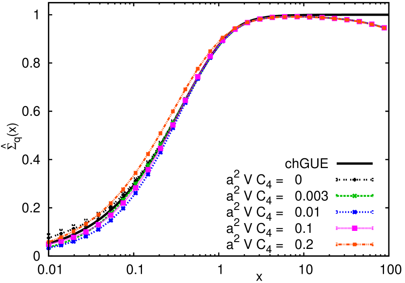
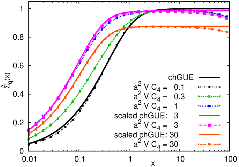
Figure 1: Quenched chiral condensate for SRMT with $N=400$ and $\nu=0$ for a range of values of $C_{4}$ in the weak (left) and strong (right) taste breaking regimes. The condensate is fairly insensitive to $C_{4}$ in the weak TB regime. In the strong TB regime it agrees well with the chiral GUE result (until finite $N$ effects set in at large $x$) with a scaled low energy constant $\Sigma_{0}^{\prime}$ given in (96).

VI.2 Quenched condensate

One of the simplest valence observables one can look at is the quenched condensate. This can still be useful for comparisons with simulations of full QCD in the case that the valence quark mass is much smaller than the dynamical masses, so that the heavier masses will simply appear quenched compared to the light valence quark.

The calculation simplifies considerably if we don’t try to calculate the corrections to the quenched partition function first, but instead directly calculate the corrections to the quenched condensate from the definition

$$\frac{\hat{\Sigma}_{q}(x)}{\Sigma_{0}}=\left.\partial_{x}\ln\hat{\cal Z}^{SRMT}_{2}(\{x,y\},\{1,-1\})\right|_{y=x}~{}.~{}$$ (68)

Applying this to (53) gives

$${\cal Z}_{x} - t_{1}\left({\cal Z}_{xxy}+{\cal Z}_{xyy}\right)-t_{3}\left({\cal Z}_{xxx}+2{\cal Z}_{xxy}+{\cal Z}_{xyy}\right)$$ (69)

$$- 2t_{2}\frac{\nu^{2}}{x^{3}}+t_{4}\left(\frac{{\cal Z}_{xx}+{\cal Z}_{xy}}{x}-\frac{{\cal Z}_{x}}{x^{2}}\right)$$

where ${\cal Z}_{x}=\partial_{x}\hat{\cal Z}_{11}(x,y)|_{y=x}$ and similarly for higher derivatives. Using the expression for the microscopic continuum partition function with $N_{f}=N_{b}=1$,

$$\hat{\cal Z}_{11}=\left|\begin{array}[]{cc}I_{\nu}(x)&xI_{\nu+1}(x)\\ -K_{\nu}(y)&yK_{\nu+1}(y)\\ \end{array}\right|~{},$$ (72)

we can now evaluate the derivatives. The result without taste breaking (${\cal Z}_{x}$) is Verbaarschot:1995yi

$$x\,[I_{\nu}(x)K_{\nu}(x)+I_{\nu+1}(x)K_{\nu-1}(x)]+\nu/x~{}.$$ (73)

If we write the final expression with TB as ${\cal Z}_{x}+\sum_{k}t_{k}z_{k}$, then we have

$$z_{1} = z_{2}=-2\nu^{2}/x^{3}$$ (74)

$$z_{3} = z_{4}+2/x-2K_{\nu}(x)[I_{\nu+1}(x)+I_{\nu-1}(x)]$$ (75)

$$z_{4} = -2K_{\nu-1}(x)I_{\nu+1}(x)/x-2\nu/x^{3}~{}.$$ (76)

Note that the single-trace TB terms enter only through the combination $t_{1}+t_{2}\propto C_{3}+C_{4}$, so that $C_{1}$ and $C_{6}$ don’t contribute while $C_{3}$ and $C_{4}$ only contribute for $\nu\neq 0$. We will see in numerical simulations below that the quenched condensate is indeed fairly insensitive to small values of $C_{4}$ for $\nu=0$.

The (partially) quenched condensate can also be used to calculate the eigenvalue density by inverting the Banks-Casher relation Banks:1979yr

$$\Sigma(m)=\frac{1}{V}\int_{-\infty}^{\infty}\frac{\rho(\lambda)}{m+i\lambda}d\lambda~{}.$$ (77)

The eigenvalue density is obtained from Osborn:1998qb

$$\rho(\lambda)=\lim_{\epsilon\to 0}\frac{\Sigma(-i\lambda+\epsilon)-\Sigma(-i\lambda-\epsilon)}{2\pi}~{}.$$ (78)

Care must be taken when evaluating $\Sigma(-i\lambda-\epsilon)$ to use the correct formula for arguments with negative real parts. We can avoid this by making use of the fact that the condensate is an odd function of $m$ (since $\rho$ is even) to get

$$\rho(\lambda)=\frac{\Sigma(i\lambda)+\Sigma(-i\lambda)}{2\pi}~{}.$$ (79)

Applying this to the quenched condensate in the microscopic limit gives the microscopic quenched eigenvalue density. The density without taste breaking is Verbaarschot:1993pm

$$\frac{\lambda}{2}\left[J_{\nu}(\lambda)^{2}-J_{\nu+1}(\lambda)J_{\nu-1}(\lambda)\right]$$ (80)

and the correction term due to taste breaking is

$$t_{3}J_{\nu}(\lambda)\left[J_{\nu-1}(\lambda)-J_{\nu+1}(\lambda)\right]-(t_{3}+t_{4})\frac{J_{\nu-1}(\lambda)J_{\nu+1}(\lambda)}{\lambda}.$$

Note that the $t_{1}$ and $t_{2}$ terms don’t contribute at this level. This expansion will also break down close to zero, similar to the condensate. Expressions that are valid near zero can be obtained from eigenvalue perturbation theory as discussed in the next section.

VI.3 Eigenvalues

The full staggered RMT is fairly complicated to work with; however, we can obtain relatively simple expressions for the effects of taste breaking on the splitting of the eigenvalues from eigenvalue perturbation theory. Since the spectrum without taste breaking contains degeneracies, we must take these into account. If $\Psi_{k}$ is a set of degenerate eigenvectors for the eigenvalue $i\lambda_{k}$,

$$({\cal D}_{0}\otimes\mathbb{I}_{4})\Psi_{k}=\Psi_{k}i\lambda_{k}~{},$$ (82)

then the eigenvalues including the leading order perturbation are given by the eigenvalues of the matrix

$$E_{k}=i\lambda_{k}+a\Psi_{k}^{\dagger}{\cal T}\Psi_{k}~{}.$$ (83)

For simplicity, we first perform a unitary similarity transformation on ${\cal D}_{0}$ to put it in the form

$$U^{\dagger}{\cal D}_{0}U=\left(\begin{array}[]{ccc}0&0&0\\ 0&0&i\Lambda\\ 0&i\Lambda&0\\ \end{array}\right)~{}.$$ (87)

with $\Lambda$ a positive diagonal matrix of the nonzero singular values of $W$. The upper left block of zeros is of size $\nu\times\nu$, representing the zero modes, while the other two blocks along the diagonal are of size $N\times N$. The above transformation can be absorbed into the taste breaking terms without changing their form, and we will not explicitly write it anymore. The nonzero eigenvalues of ${\cal D}_{0}$ written as $\lambda_{k}$ above are simply plus or minus the diagonal elements of $\Lambda$. In this basis the eigenvectors take the form

$$\Psi=\frac{1}{\sqrt{2}}\left(\begin{array}[]{ccc}\sqrt{2}\mathbb{I}_{\nu}&0&0\\ 0&\mathbb{I}_{N}&\mathbb{I}_{N}\\ 0&\mathbb{I}_{N}&-\mathbb{I}_{N}\\ \end{array}\right)\otimes\mathbb{I}_{4}~{}.$$ (91)

We first examine the sector of the $4\nu$ zero modes for which we define $k=0$. The matrix $E_{0}$ is just a projection onto the upper left $\nu\times\nu$ block for all tastes of the taste breaking term. This gives the form

$$i(A_{3\mu}+b_{V\mu}+c_{V\mu})\otimes\xi_{\mu}+(A_{4\mu}+b_{A\mu}+c_{A\mu})\otimes\xi_{\mu 5}~{}~{}~{}~{}~{}~{}~{}$$ (92)

with implied summation over $\mu$. The $A$’s are $\nu\times\nu$ Hermitian matrices and the $b$’s and $c$’s are real scalars (as given in Appendix B). The terms are labeled according to their origin in the full SRMT and have the same Gaussian weights as the corresponding terms in the full SRMT. Here we see that only the pseudoscalar and tensor terms don’t affect the splittings of the zero modes. Also, if we ignore the scalars and were to set $C_{3}=C_{4}$, then the would-be zero modes are described by a chiral RMT, for which the eigenvalues are readily found. However, typically we have that $C_{4}\gg C_{3}$ so that, to a good approximation, we can set $C_{3}=0$, which will give a different distribution for the eigenvalues.

We now examine the splitting within a degenerate quartet of eigenvalues. Here the $4\times 4$ splitting matrix, $\Psi_{k}^{\dagger}{\cal T}\Psi_{k}$, has the form

$$id_{1}\otimes\xi_{5}+d_{6\mu\nu}\otimes\xi_{\mu\nu} + ix_{V\mu}\otimes\xi_{\mu}+x_{A\mu}\otimes\xi_{\mu 5}$$ (93)

with $x_{V\mu}=d_{3\mu}+b_{V\mu}$ and $x_{A\mu}=d_{4\mu}+b_{A\mu}$. All the $d$’s are real scalars; again they are labeled according to their origin, and their weight is $\exp(-\alpha N^{2}d_{X}^{2}/VC_{X})$. Since the $d_{1,3,4,6}$ terms came from matrices in the original SRMT, they are different for each quartet. However, the $b_{A,V}$ terms came from scalars in the SRMT, so these variables are in fact the same in all quartets, and also in the zero mode sector. It is these terms that produce the leading order eigenvalue correlations between the different quartets and also allow the splittings within each quartet to be sensitive to the topological charge in the weak TB regime. Interestingly these are the terms in staggered chiral perturbation theory which don’t contribute at one loop.

In Sec. VI.1 we gave an expression for the partition function that could become singular as $m\to 0$. Using the eigenvalues from perturbation theory we can derive a similar expression that treats the zero modes exactly. Since the $O(a)$ correction to the quark determinant vanishes, we need to go to second order in eigenvalue perturbation theory. The expression for the eigenvalues in second order degenerate eigenvalue perturbation theory is

$$E_{k}=i\lambda_{k}+a\Psi_{k}^{\dagger}{\cal T}\Psi_{k}-ia^{2}\sum_{\ell\neq k}\frac{\Psi_{k}^{\dagger}{\cal T}\Psi_{\ell}\Psi_{\ell}^{\dagger}{\cal T}\Psi_{k}}{\lambda_{k}-\lambda_{\ell}}~{}.$$ (94)

We can obtain an expression for the quark determinant (and hence the partition function) which is accurate to order $a^{2}$ by multiplying the determinants of the $E_{k}$. If the determinants for each quartet were expanded in $a$, we would obtain an expression for the partition function identical to (53). However, to produce an expression that is valid at $m=0$, the determinants must be handled exactly. We will not deal with that here.

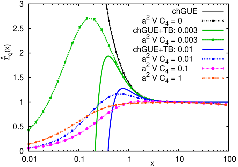
Figure 2: Quenched chiral condensate for SRMT with $N=400$ and $\nu=1$ for a range of values of $C_{4}$ in the weak taste breaking regime.

VII Strong taste breaking

Earlier we showed how the fermionic SRMT partition function maps onto the staggered chiral Lagrangian for weak taste breaking. There we took the large $N$ limit of the SRMT while scaling the terms $a^{2}\alpha/\beta\sim 1/N$. This means that the $a^{2}VC_{X}$ terms are kept fixed as $N,V\to\infty$. Now we consider a different limit where the $C_{X}$ are kept fixed so that $a^{2}\alpha/\beta$ stays constant in the large $N$ limit. Here the taste breaking must be included in the saddle point equations when going from the sigma model to the chiral Lagrangian, as mentioned in Appendix A. The inclusion of TB breaks the Goldstone manifold from SU(4) down to U(1). Note that if only $C_{1}\neq 0$ then the symmetry is not fully broken down to U(1), but since that is not a likely scenario for common staggered actions, we will not consider it further.

The result for the effective chiral Lagrangian in the strong TB regime is

$${\cal L}=-\frac{1}{2}\Sigma_{0}^{\prime}m(U+U^{\dagger})$$ (95)

where $U\in U(1)$. This has the form of a single fermionic flavor with a modified condensate given by

$$\Sigma_{0}^{\prime}=\frac{4\Sigma_{0}}{\sqrt{1+a^{2}\bar{D}}}~{}.$$ (96)

with $a^{2}\bar{D}=a^{2}V\bar{C}/N$. The factor of 4 is due to the four tastes, and the TB terms serve to decrease the effective condensate.

Note that this result differs from what we would obtain from the large TB limit of the weak TB Lagrangian. That is, if we start with the Lagrangian (4) and take the saddle point in the non-Goldstone modes as $a^{2}\to\infty$ (or equivalently keeping the $C$’s fixed as $V\to\infty$), we would get the same form for the effective Lagrangian as in (95) but with a condensate that is simply $\Sigma_{0}^{\prime}=4\Sigma_{0}$. This is because in the weak TB limit $\bar{D}$ would be scaled to zero, while it remains finite in the strong TB limit. Thus, in general, the two limits should be considered distinct even though some observables may exhibit a smooth transition between them. We will explore this transition from weak to strong TB through numerical simulations of the SRMT.

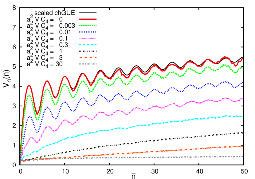
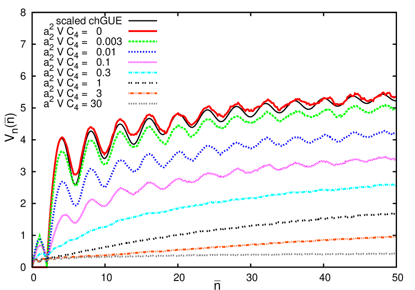
Figure 3: Number variance for the SRMT with $N=400$ and $\nu=0$, left ($\nu=1$, right), for a range of values of $C_{4}$ showing the transition from weak to strong taste breaking.

VIII Numerical results

Here we present some numerical results obtained from averaging over 10,000 random matrix configurations obtained with $N=400$ (and setting $\alpha=1$) at both $\nu=0$ and $\nu=1$. We varied the value of $c=a^{2}VC_{4}$ from 0 to 100, and all other TB coefficients were set to zero.

In Fig. 1 we plot the quenched condensate from the SRMT. In the left panel, the taste breaking parameter $c$ is varied between $0$ and $0.2$. For $c=0$ we find the expected agreement with the plotted result from the chiral GUE (chGUE), Eq. (73), for small $x$. For larger $x$ we see a discrepancy due to the finite $N$ of the SRMT. As $N$ is increased, the SRMT results will rise to match the chGUE curve. As $c$ is increased, we see some small changes in the quenched condensate for small $x$, but not for larger $x$. This is in agreement with our expectations from the expansion (74) since we don’t expect it to be valid near $x=0$. At $c\approx 0.2$ we start to see changes in the condensate at larger $x$, signaling the end of the weak TB approximation.

On the right panel of Fig. 1, we show the quenched condensate as it leaves the weak TB regime and goes to the strong one. The scaled chGUE results shown are given by (normalized to a single flavor)

$$\hat{\Sigma}_{q}^{\mathrm{strong}}(x)=\frac{s}{4}\hat{\Sigma}_{q}^{\mathrm{chGUE}}(sx)$$ (97)

with $s=\Sigma_{0}^{\prime}/\Sigma_{0}$ and using Eq. (96). For $c>1$ we see very good agreement between the SRMT results and the above formula, until the finite $N$ effects set in at large $x$.

In Fig. 2 we plot the quenched condensate at $\nu=1$ in the weak TB regime. The chiral GUE result has an explicit $\nu/x$ divergence which is matched by the $C_{4}=0$ data. As $C_{4}$ is increased, the expansion of the condensate gives a TB correction proportional to $-\nu^{2}/x^{3}$ [Eq. (74)]. This corrected GUE result agrees with the data at $c=0.003$ for $x>0.5$, while at $c=0.01$ the agreement is found only for approximately $x>2$. For larger $c$ the expansion breaks down. At large $c>1$ the $\nu=1$ quenched condensate enters the strong TB regime and will match the strong TB result of the $\nu=0$ sector.

As previously mentioned, the chiral condensate is related to the eigenvalue density. Next we will look at the number variance which is related to the two-point eigenvalue correlation function. It is defined as

$$V_{n}(\bar{n})=\langle\langle\left[n(\bar{n})-\bar{n}\right]^{2}\rangle\rangle$$ (98)

where $\langle\langle\cdot\rangle\rangle$ denotes the ensemble average. The function $n(\bar{n})$ is the number of eigenvalues between $0$ and $\ell$ in a particular configuration with $\ell$ chosen such that the interval has on average $\bar{n}$ eigenvalues.

In Fig. 3 we plot the number variance for a range of values of $C_{4}$, with all other coefficients set to zero at both $\nu=0$ and $\nu=1$ topological charges. At $C_{4}=0$ the number variance matches that of the chiral GUE ($V_{n}^{\mathrm{chGUE}}$) Ma:1997zp , after the appropriate scaling

$$V_{n}^{C_{4}=0}(\bar{n})=16V_{n}^{\mathrm{chGUE}}([\bar{n}-2\nu]/4)$$ (99)

due to the fourfold degeneracy of the spectrum and the zero modes. Note that at $C_{4}=0$ there are really $4\nu$ exact zero modes; however, we are considering this to be the limit of $C_{4}\to 0^{+}$, where for small $C_{4}>0$ the zero modes are split into $2\nu$ positive and negative near-zero modes. This gives a shift of the number variance by $2\nu$.

As $C_{4}$ moves away from zero, we see the number variance drop while retaining the same pattern of oscillations until $a^{2}VC_{4}\approx 0.3$. Here the large oscillations have essentially vanished. Upon increasing $C_{4}$ the number variance continues to decrease and a set of smaller oscillations appear that coincide with the result from the one flavor chiral GUE without any scaling.

In Fig. 4 we can see the transition to the strong TB regime from the same data. As $C_{4}$ is increased a larger range of the data falls on top of the chiral GUE curve. The point where the data starts to deviate from the chGUE curve is roughly equivalent to the value of $a^{2}VC_{4}$. For example for $a^{2}VC_{4}=10$, the number variance agrees with the chGUE result up to around $\bar{n}=10$, above which it begins to grow larger than the chGUE curve. This is similar to what one sees around the Thouless energy Osborn:1998nm ; Osborn:1998nf ; however, in this case it does not signal the breakdown of the RMT, but is instead the signal of the restoration of an explicitly broken symmetry (taste). The behavior is independent of the value of $N$. If one observed a similar behavior of the number variance in lattice simulations, this could provide an independent estimate of the size of taste breaking.

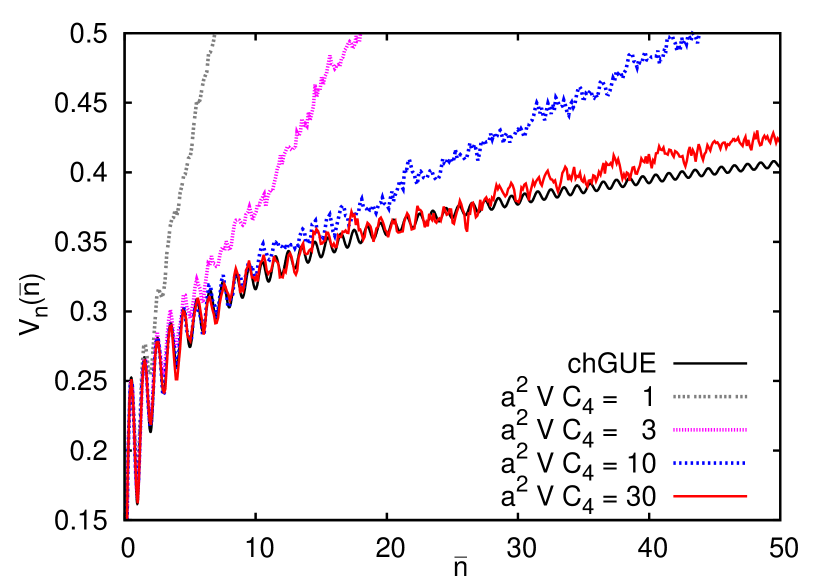
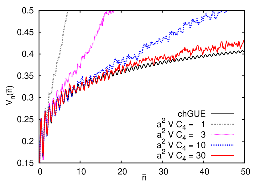
Figure 4: Number variance for SRMT with $N=400$ and $\nu=0$, left ($\nu=1$, right), for a range of values of $C_{4}$ in the strong taste breaking regime.

IX Summary and future work

We have presented a completed chiral random matrix theory for staggered fermions that includes all the taste breaking effects at order $a^{2}$. The SRMT has been shown to be equivalent to the zero-momentum staggered chiral Lagrangian in the appropriate limit. We have also identified a strong taste breaking limit where the SRMT maps onto a one flavor effective Lagrangian.

The quenched condensate and number variance evaluated in the SRMT, clearly show the transition from the weak to the strong taste breaking regime. The number variance is particularly interesting since for strong TB, the TB scale $a^{2}V\bar{C}$ seems to be directly related to the range of agreement to the one flavor chiral GUE result. We now need to test the results of the SRMT against lattice simulations with staggered fermions.

One could also extend the SRMT to include an imaginary quark chemical potential. This can then be used to obtain a measurement of the low energy constant $F$ Damgaard:2005ys ; Damgaard:2006pu ; Damgaard:2006rh ; Akemann:2006ru ; Akemann2008406 and could potentially provide more information on the taste breaking. Similarly one could add a real chemical potential and study the effects of taste breaking on the complex eigenvalues Osborn:2004rf ; Akemann:2004dr . Additionally, one could explore the problems associated with rooting when the quark determinant is complex Golterman:2006rw ; Svetitsky:2006sn .

Appendix A Mapping the SRMT to the staggered chiral Lagrangian

The procedure for mapping the chiral RMT onto the zero-momentum chiral Lagrangian is by now standard Shuryak:1992pi ; Basile:2007ki . Here we will consider the case of only fermions, and will leave the addition of bosonic quarks (ghosts) for later.

We introduce a set of Grassmann variables $\psi^{ts}_{i}$ and $\bar{\psi}^{ts}_{i}$, with $t$ the taste index, $s=\pm$ the chiral index, and $i$ the random matrix index. The determinant can then be written as

$$\det({\cal D}_{0}+m+a{\cal T}) = \int d\bar{\psi}d\psi\mathrm{e}^{\bar{\psi}({\cal D}_{0}+m+a{\cal T})\psi}$$

$$= \int d\bar{\psi}d\psi\mathrm{e}^{m\bar{\psi}\psi-\left\langle({\cal D}_{0}+a{\cal T})\psi\bar{\psi}\right\rangle}~{}.$$

In this form the Gaussian integrals over the random matrices can be readily performed. This leads to a set of four fermion terms in the exponential. For the terms with scalars instead of matrices, we do not need to perform the Gaussian integrals now, and can wait until after expanding around the saddle point below. We will consider the different types of taste breaking terms separately, and in each case the Gaussian measure is taken to be

$$\exp(-\beta N\left\langle{\cal T}^{\dagger}{\cal T}\right\rangle/4)~{}.$$ (101)

The four fermion terms generated by the two types of terms with random matrices considered can be summarized as follows:

$$\left(\begin{array}[]{cc}0&iX\\ iX^{\dagger}&0\\ \end{array}\right)\otimes\Gamma \to \frac{a^{2}}{\beta N}\left\langle\bar{\psi}^{i+}\psi^{j+}\Gamma_{kj}\bar{\psi}^{k-}\psi^{\ell-}\Gamma_{i\ell}\right\rangle$$ (104)

$$\left(\begin{array}[]{cc}iA&0\\ 0&iB\\ \end{array}\right)\otimes\Gamma \to \frac{a^{2}}{\beta N}\sum_{s=\pm}\left\langle\bar{\psi}^{is}\psi^{js}\Gamma_{kj}\bar{\psi}^{ks}\psi^{\ell s}\Gamma_{i\ell}\right\rangle.~{}~{}~{}~{}~{}~{}$$ (107)

These can be transformed into fermion bilinears by the Hubbard-Stratonovich transformation, yielding

$$\exp(-\beta N\left\langle\rho^{\dagger}\rho\right\rangle+a\bar{\psi}^{+}\rho\Gamma\psi^{+}+a\bar{\psi}^{-}\rho^{\dagger}\Gamma\psi^{-})$$ (108)

$$\exp(-\beta N\left\langle\rho_{+}^{2}+\rho_{-}^{2}\right\rangle+a\bar{\psi}^{+}\rho_{+}\Gamma\psi^{+}+a\bar{\psi}^{-}\rho_{-}\Gamma\psi^{-})~{}~{}~{}~{}~{}~{}$$ (109)

respectively, where $\rho$ is a $4\times 4$ complex matrix and $\rho_{\pm}$ are $4\times 4$ Hermitian. The Grassmann integrals can now be performed yielding a determinant.

In the absence of taste breaking, the RMT at this point would be

$$\int d\sigma\det(\sigma+m)^{N+\nu}\det(\sigma^{\dagger}+m)^{N}\mathrm{e}^{-\alpha N\left\langle\sigma^{\dagger}\sigma\right\rangle}~{}$$ (110)

with $\sigma$ a $4\times 4$ complex matrix. In the large $N$ limit, keeping $\sqrt{\alpha}mN$ fixed (the microscopic limit) one finds the saddle point solution of $\sigma=U/\sqrt{\alpha}$, where $U$ is a unitary matrix. The partition function expanded around this solution then becomes

$$\int dU\det(U)^{\nu}\exp(\sqrt{\alpha}mN\left\langle U+U^{\dagger}\right\rangle)~{}.$$ (111)

Matching to the chiral Lagrangian we get $\sqrt{\alpha}=\Sigma_{0}V/2N$.

To include the TB terms we must first choose how to scale those terms with $N$. If we had scaled the matrix $\rho$ to have the same Gaussian weight as $\sigma$, then we would get for (108)

$$\exp(-\alpha N\left\langle\rho^{\dagger}\rho\right\rangle+a\sqrt{\alpha/\beta}[\bar{\psi}^{+}\rho\Gamma\psi^{+}+\bar{\psi}^{-}\rho^{\dagger}\Gamma\psi^{-}]).~{}~{}~{}~{}~{}$$ (112)

The scaling of the term $a\sqrt{\alpha/\beta}$ determines whether we are in the weak or strong TB regimes. If it is held constant then the term with $\rho$ in the determinant will have a similar magnitude as the term with $\sigma$ and we must include it in the saddle point equations.

For this strong TB regime, at the saddle point we find, for the term given in (108),

$$\rho=(a/\beta)\Gamma\sigma^{\dagger-1}$$ (113)

and in (109),

$$\rho_{+} = (a/2\beta)\Gamma\sigma^{-1}$$ (114)

$$\rho_{-} = (a/2\beta)\Gamma\sigma^{\dagger-1}~{}.$$ (115)

The two-trace TB terms do not contribute to the saddle point. The saddle point solution for $\sigma$ has the form

$$\sigma=c\exp(i\xi_{5}\theta)$$ (116)

for some $c$. The resulting effective Lagrangian for the strong TB limit of the SRMT is given in (95) with $U=\exp(i\theta)$.

For weak taste breaking we can take $a\sqrt{\alpha/\beta}\sim 1/\sqrt{N}$. Then the saddle point solution is unchanged by taste breaking and the TB terms can be expanded around the saddle point solution. Then the remaining Gaussian integrals can easily be performed, yielding the set of terms given in Table 1.

Appendix B SRMT

For completeness, we will explicitly write down all the taste breaking terms from the full staggered RMT. The SRMT Dirac matrix is given by the form in Eq. (15). The taste breaking terms ${\cal T}$ are given by the sum of the following terms:

$${\cal T}_{1} = \left(\begin{array}[]{cc}0&iX_{1}\\ iX_{1}^{\dagger}&0\end{array}\right)\otimes\xi_{5}$$ (119)

$${\cal T}_{3} = \sum_{\mu}\left(\begin{array}[]{cc}iA_{3\mu}&0\\ 0&iB_{3\mu}\end{array}\right)\otimes\xi_{\mu}$$ (122)

$${\cal T}_{4} = \sum_{\mu}\left(\begin{array}[]{cc}A_{4\mu}&0\\ 0&B_{4\mu}\end{array}\right)\otimes\xi_{\mu 5}$$ (125)

$${\cal T}_{6} = \sum_{\mu<\nu}\left(\begin{array}[]{cc}0&X_{6\mu\nu}\\ X_{6\mu\nu}^{\dagger}&0\end{array}\right)\otimes\xi_{\mu\nu}$$ (128)

$${\cal T}_{V}^{+} = \sum_{\mu}\left(\begin{array}[]{cc}ib_{V\mu}&0\\ 0&ib_{V\mu}\end{array}\right)\otimes\xi_{\mu}$$ (131)

$${\cal T}_{V}^{-} = \sum_{\mu}\left(\begin{array}[]{cc}ic_{V\mu}&0\\ 0&-ic_{V\mu}\end{array}\right)\otimes\xi_{\mu}$$ (134)

$${\cal T}_{A}^{+} = \sum_{\mu}\left(\begin{array}[]{cc}b_{A\mu}&0\\ 0&b_{A\mu}\end{array}\right)\otimes\xi_{\mu 5}$$ (137)

$${\cal T}_{A}^{-} = \sum_{\mu}\left(\begin{array}[]{cc}c_{A\mu}&0\\ 0&-c_{A\mu}\end{array}\right)\otimes\xi_{\mu 5}$$ (140)

The Gaussian weights for the individual terms are

$$\exp \Bigg{(} \frac{\alpha N^{2}}{8V}\left[\left\langle\frac{{\cal T}_{1}^{2}}{C_{1}}+\frac{{\cal T}_{3}^{2}}{C_{3}}+\frac{{\cal T}_{4}^{2}}{C_{4}}+\frac{{\cal T}_{6}^{2}}{C_{6}}\right\rangle\right]$$ (141)

$$- \frac{\alpha N^{2}}{V}\sum_{\mu}\left[\frac{b_{V\mu}^{2}}{C_{V}^{+}}+\frac{c_{V\mu}^{2}}{C_{V}^{-}}+\frac{b_{A\mu}^{2}}{C_{A}^{+}}+\frac{c_{A\mu}^{2}}{C_{A}^{-}}\right]\Bigg{)}~{}.$$

References

- (1) W.-J. Lee and S. R. Sharpe, Phys. Rev. D60, 114503 (1999), arXiv:hep-lat/9905023
- (2) C. Aubin and C. Bernard, Phys. Rev. D68, 034014 (2003), arXiv:hep-lat/0304014
- (3) J. C. Osborn, Nucl. Phys. Proc. Suppl. 129, 886 (2004), arXiv:hep-lat/0309123
- (4) M. A. Halasz and J. J. M. Verbaarschot, Phys. Rev. Lett. 74, 3920 (1995), arXiv:hep-lat/9501025
- (5) H. Kluberg-Stern, A. Morel, O. Napoly, and B. Petersson, Nucl. Phys. B220, 447 (1983)
- (6) E. V. Shuryak and J. J. M. Verbaarschot, Nucl. Phys. A560, 306 (1993), arXiv:hep-th/9212088
- (7) S. Nishigaki, Phys. Lett. B387, 139 (1996), arXiv:hep-th/9606099
- (8) G. Akemann, P. H. Damgaard, U. Magnea, and S. Nishigaki, Nucl. Phys. B487, 721 (1997), arXiv:hep-th/9609174
- (9) J. J. M. Verbaarschot and T. Wettig, Ann. Rev. Nucl. Part. Sci. 50, 343 (2000), arXiv:hep-ph/0003017
- (10) J. C. Osborn, D. Toublan, and J. J. M. Verbaarschot, Nucl. Phys. B540, 317 (1999), arXiv:hep-th/9806110
- (11) P. H. Damgaard, J. C. Osborn, D. Toublan, and J. J. M. Verbaarschot, Nucl. Phys. B547, 305 (1999), arXiv:hep-th/9811212
- (12) F. Basile and G. Akemann, JHEP 12, 043 (2007), arXiv:0710.0376 [hep-th]
- (13) J. Gasser and H. Leutwyler, Phys. Lett. B188, 477 (1987)
- (14) P. H. Damgaard, K. Splittorff, and J. J. M. Verbaarschot(2010), arXiv:1001.2937 [hep-th]
- (15) G. Akemann, P. H. Damgaard, K. Splittorff, and J. J. M. Verbaarschot(2010), arXiv:1012.0752 [hep-lat]
- (16) C. Aubin et al. (MILC), Phys. Rev. D70, 114501 (2004), arXiv:hep-lat/0407028
- (17) M. E. Berbenni-Bitsch, S. Meyer, A. Schafer, J. J. M. Verbaarschot, and T. Wettig, Phys. Rev. Lett. 80, 1146 (1998), arXiv:hep-lat/9704018
- (18) P. H. Damgaard, U. M. Heller, and A. Krasnitz, Phys. Lett. B445, 366 (1999), arXiv:hep-lat/9810060
- (19) M. Gockeler, H. Hehl, P. E. L. Rakow, A. Schafer, and T. Wettig, Phys. Rev. D59, 094503 (1999), arXiv:hep-lat/9811018
- (20) P. H. Damgaard, U. M. Heller, R. Niclasen, and K. Rummukainen, Phys. Rev. D61, 014501 (1999), arXiv:hep-lat/9907019
- (21) E. Follana, A. Hart, and C. T. H. Davies (HPQCD), Phys. Rev. Lett. 93, 241601 (2004), arXiv:hep-lat/0406010
- (22) S. Durr, C. Hoelbling, and U. Wenger, Phys. Rev. D70, 094502 (2004), arXiv:hep-lat/0406027
- (23) E. Follana, A. Hart, C. T. H. Davies, and Q. Mason (HPQCD), Phys. Rev. D72, 054501 (2005), arXiv:hep-lat/0507011
- (24) J. C. Osborn and J. J. M. Verbaarschot, Nucl. Phys. B525, 738 (1998), arXiv:hep-ph/9803419
- (25) J. C. Osborn and J. J. M. Verbaarschot, Phys. Rev. Lett. 81, 268 (1998), arXiv:hep-ph/9807490
- (26) K. Splittorff and J. J. M. Verbaarschot, Phys. Rev. Lett. 90, 041601 (2003), arXiv:cond-mat/0209594
- (27) Y. V. Fyodorov and G. Akemann, JETP Lett. 77, 438 (2003), arXiv:cond-mat/0210647
- (28) J. J. M. Verbaarschot, Phys. Lett. B368, 137 (1996), arXiv:hep-ph/9509369
- (29) T. Banks and A. Casher, Nucl. Phys. B169, 103 (1980)
- (30) J. J. M. Verbaarschot and I. Zahed, Phys. Rev. Lett. 70, 3852 (1993), arXiv:hep-th/9303012
- (31) J.-Z. Ma, T. Guhr, and T. Wettig, Eur. Phys. J. A2, 87 (1998), arXiv:hep-lat/9712026
- (32) P. H. Damgaard, U. M. Heller, K. Splittorff, and B. Svetitsky, Phys. Rev. D72, 091501 (2005), arXiv:hep-lat/0508029
- (33) P. H. Damgaard, U. M. Heller, K. Splittorff, B. Svetitsky, and D. Toublan, Phys. Rev. D73, 074023 (2006), arXiv:hep-lat/0602030
- (34) P. H. Damgaard, U. M. Heller, K. Splittorff, B. Svetitsky, and D. Toublan, Phys. Rev. D73, 105016 (2006), arXiv:hep-th/0604054
- (35) G. Akemann, P. H. Damgaard, J. C. Osborn, and K. Splittorff, Nucl. Phys. B766, 34 (2007), arXiv:hep-th/0609059
- (36) G. Akemann, P. Damgaard, J. Osborn, and K. Splittorff, Nuclear Physics B 800, 406 (2008)
- (37) J. C. Osborn, Phys. Rev. Lett. 93, 222001 (2004), arXiv:hep-th/0403131
- (38) G. Akemann, J. C. Osborn, K. Splittorff, and J. J. M. Verbaarschot, Nucl. Phys. B712, 287 (2005), arXiv:hep-th/0411030
- (39) M. Golterman, Y. Shamir, and B. Svetitsky, Phys. Rev. D74, 071501 (2006), arXiv:hep-lat/0602026
- (40) B. Svetitsky, Y. Shamir, and M. Golterman, PoS LAT2006, 148 (2006), arXiv:hep-lat/0609051