Symmetry Principles in Quantum Systems Theory

Abstract

General dynamic properties like controllability and simulability of spin systems, fermionic and bosonic systems are investigated in terms of symmetry. Symmetries may be due to the interaction topology or due to the structure and representation of the system and control Hamiltonians. In either case, they obviously entail constants of motion. Conversely, the absence of symmetry implies irreducibility and provides a convenient necessary condition for full controllability much easier to assess than the well-established Lie-algebra rank condition. We give a complete lattice of irreducible simple subalgebras of $\mathfrak{su}(2^{n})$ for up to $n=15$ qubits. It complements the symmetry condition by allowing for easy tests solving homogeneous linear equations to filter irreducible unitary representations of other candidate algebras of classical type as well as of exceptional types. — The lattice of irreducible simple subalgebras given also determines mutual simulability of dynamic systems of spin or fermionic or bosonic nature. We illustrate how controlled quadratic fermionic (and bosonic) systems can be simulated by spin systems and in certain cases also vice versa.

1 Introduction

Experimental control over quantum dynamics of manageable systems is paramount to exploiting the great potential of quantum systems. Both in simulation and computation the complexity of a problem may reduce upon going from a classical to a quantum setting [1, 2, 3]. On the computational end, where quantum algorithms efficiently solving hidden subgroup problems [4] have established themselves, the demands for accuracy (‘error-correction threshold’) may seem daunting at the moment. In contrast, the quantum simulation end is by far less sensitive. Thus simulating quantum systems [5]—in particular at phase-transitions [6, 7]—has recently shifted into focus [8, 9, 10, 11, 12]. In view of experimental progress in cold atoms in optical lattice potentials [13, 14] as well as in trapped ions [15, 16], Kraus et al. have explored whether target quantum systems can be universally simulated on translationally invariant lattices of bosonic, fermionic, and spin systems [17]. In some respect, their work can also be seen as a follow-up on a study by Schirmer et al. [18] (see also recent work by Wang et al. [19]) specifically addressing controllability of systems with degenerate transition frequencies. Many experimental tasks are engineering problems that profit from quantum systems theory as a framework and optimal control algorithms for solving the actual problem.

As compared to an abstract point of view [20], the flavour of quantum systems theory pursued here is meant to be very pragmatic: it takes the causal formulation of dynamic systems [21] and does not care about specifics of the quantum measurement problem beyond the basic notions [22] and some recent developments [23]. Yet it is for these reasons that quantum systems and control has quite generally been recognised as a key generic tool [24, 25, 26] needed for advances in experimentally exploiting quantum systems for simulation or computation and even more so in future quantum technology. It paves the way for constructively optimising strategies for experimental implementions in realistic settings. Moreover, since such realistic quantum systems are mostly beyond analytical tractability, numerical methods are often indispensable. To this end, gradient flows can be implemented on the control amplitudes thus iterating an initial guess into an optimised pulse scheme [27, 28, 29]. This approach has proven useful in spin systems [30] as well as in solid-state systems [31]. Moreover, it has recently been generalised from closed systems to open ones [32], which are known to be a challenge to control [33], where the Markovian setting can also be used as embedding of explicitly non-Markovian subsystems [34].

However, in closed systems, the numerical tools usually require the system is universal or fully operator controllable [35, 36]. For a plethora of systems with symmetry constraints we have recently determined explicit dynamic system algebras [37] (as subalgebras of $\mathfrak{su}(N)$), and conversely, we have derived design rules for the experimenter as guidelines ensuring universality of quantum architecture. While extending earlier work on branching diagrams of simple subalgebras of $\mathfrak{su}(N)$ [38, 39], here we focus on complete necessary and sufficient conditions for full controllability (mostly) confining ourselves to arguments easy to check by inspection or to decide by computationally cheap algorithms such as solving a system of homogeneous linear equations.

In view of applications, we illustrate our findings by a comprehensive set of worked examples on spin chains. Actually Ising-${\sf ZZ}$ coupled $n$-spin-$\tfrac{1}{2}$ chains with mostly collective controls or Heisenberg-${\sf XX}$ chains with one single local control suffice to get exponential growth of dynamic degrees of freedom (in the sense their respective dynamic system algebras are $\mathfrak{sp}(2^{n-1})$ or $\mathfrak{so}(2^{n})$). Our work thus adds to the recent spin-chain literature (see, e.g., [40, 41, 42, 43, 44, 45, 46, 47, 48, 19] and compare [49, 50, 51]) and—on a more general scale—it is anticipated to have significant impact on quantum simulation as well as distributed quantum computing (see, e.g., [52, 53, 54]).

2 Overview and Main Results

More precisely, the first main part develops, starting from the basic notions of controllability (Sec. 3) in terms of coupling graphs (Sec. 4) and their symmetries (Sec. 5), a single necessary and sufficient symmetry condition for full controllability (Sec. 7). To this end and in view of practical applications, Sec. 6 gives branching diagrams of all irreducible simple subalgebras of the unitary algebras $\mathfrak{su}(N)$ with $N\leq 2^{15}$. Concomitantly, we provide a set of efficient computational algorithms for assessing controllability by merely solving systems of homogeneous linear equations.

The second part focusses on simulability (Sec. 8) in terms of dynamic system algebras. A plethora of worked examples is discussed in Sec. 9 including four full series of qubit chains coupled by pair interactions such that their dynamic system algebras for the first three cases are $\mathfrak{so}(2n+1)$, $\mathfrak{so}(2n+2)$, and $\mathfrak{sp}(2^{n-1})$, respectively. Most remarkably, for $n\geq 4$, the fourth series results in dynamic system algebras $\mathfrak{so}(2^{n})$ if $(n\bmod{4})\in\{0,1\}$ and $\mathfrak{sp}(2^{n-1})$ else. The findings also interrelate spin systems, fermionic systems (Sec. 10) and bosonic systems (Sec. 11). The algebraic conditions for simulability given are sufficient to ensure the existence of solutions to the actual task of quantum simulation of closed systems formulated as an observed optimal control problem in the outlook (Sec. 12).

3 Controllability

Consider the controlled Schrödinger equation lifted to unitary maps (quantum gates)

$${\dot{U}(t)}=-i\big{(}H_{d}+\sum_{j=1}^{m}u_{j}(t)H_{j}\big{)}\;{U(t)}\;.$$ (1)

Here the system Hamiltonian $H_{d}$ denotes a non-switchable drift term and the control Hamiltonians $H_{j}$ can be steered by (piece-wise constant) control amplitudes $u_{j}(t)\in\mathbb{R}$ taken to be unbounded henceforth. The equation of motion governs the evolution of a unitary map of an entire basis set of vectors representing pure states. Using the short-hand notations $H:=H_{d}+\sum_{j=1}^{m}u_{j}(t)H_{j}$ and $\operatorname{ad}_{H}(\operatorname{vec}{A}):=[H,A]$, the Liouville equation $\dot{\rho}(t)=-i[H,\rho(t)]$ can be rewritten

$$\operatorname{vec}{\dot{\rho}(t)}=-i\operatorname{ad}_{H}\operatorname{vec}{\rho(t)}.$$ (2)

Both equations of motion take the form of a standard bilinear control system $(\Sigma)$ known in classical systems and control theory [55]

$$\dot{X}(t)=\big{(}A+\sum_{j=1}^{m}u_{j}(t)B_{j}\big{)}\;X(t)$$ (3)

with ‘state’ $X(t)\in\mathbb{C}^{N}$, drift $A\in\mathfrak{gl}(N,\mathbb{C})$, controls $B_{j}\in\mathfrak{gl}(N,\mathbb{C})$, and control amplitudes $u_{j}\in\mathbb{R}$, where $\mathfrak{gl}(N,\mathbb{C})$ denotes the set of complex $N\times N$ matrices. Since all the control systems considered henceforth are bilinear, we often drop the specification bilinear for short. Now lifting the (bilinear) control system $(\Sigma)$ to group manifolds [56, 57] by $X(t)\in\mathrm{GL}(N,\mathbb{C})$, i.e. the set of non-singular complex $N\times N$ matrices, under the action of a compact connected Lie group $\mathbf{K}$ with Lie algebra $\mathfrak{k}$ while keeping $A,B_{j}\in\mathfrak{gl}(N,\mathbb{C})$, the condition for full controllability turns into the Lie algebra rank condition [58, 59, 57]

$$\langle A,B_{j}\,|\,j=1,2,\dots,m\rangle_{\rm Lie}=\mathfrak{k},$$ (4)

where $\langle\cdot\rangle_{\rm Lie}$ denotes (the linear span over) the Lie closure obtained by repeatedly taking mutual commutator brackets. Algorithm 1 gives an explicit method to compute the Lie closure, see also [60].

Algorithm 1: Determine system algebra via Lie closure
	Input: Hamiltonians $I:=\{iH_{d};iH_{1},\dots,iH_{m}\}\subseteq\mathfrak{su}(N)$
	1. $B:=$ maximal linearly independent subset of $I$
	2. $\mathrm{num}:=\#B$
	3. If $\mathrm{num}=N$ then $O:=B$ else $O:=\{\,\}$
	4. If $\mathrm{num}=N$ or $\#B=0$ then terminate
	5. $C:=[O,B]\cup[B,B]$, where
	5. $[S_{1},S_{2}]=\{[s_{1},s_{2}]\,|\,s_{1}\in S_{1},s_{2}\in S_{2}\}$
	6. $O:=O\cup B$
	7. $B:=$ max. linear independent extension of $O$
	7. with elements from $C$
	8. $\mathrm{num}:=\mathrm{num}+\#B$; Go to 4
	Output: basis $O$ of the generated Lie algebra and
	Output: its dimension $\mathrm{num}$
	The complexity is roughly $\mathcal{O}(N^{6}\cdot N^{2})$, as about $N^{2}$ times
	a rank-revealing $QR$ decomposition has to be performed in
	Liouville space (with dimension $N^{2}$). For $n$ qubits, $N:=2^{n}$.

Transferring the classical result [59] to the quantum domain [61, 62, 36], the bilinear system of Eqn. (1) is fully (operator) controllable if and only if the drift and controls are a generating set of the special unitary algebra $\mathfrak{su}(N)$:

$$\langle{iH_{d},iH_{j}}\,|\,j=1,2,\dots,m\rangle_{\rm Lie}=\mathfrak{k}=\mathfrak{su}(N).$$ (5)

In fully controllable systems, to every initial state $\rho_{0}$ the reachable set is the entire unitary orbit $\mathcal{O}_{\rm U}(\rho_{0}):=\{U\rho_{0}U^{\dagger}\;|\;U\in\operatorname{SU}(N)\}$. With density operators being Hermitian this means any final state $\rho(t)$ can be reached from any initial state $\rho_{0}$ as long as both of them share the same spectrum of eigenvalues. Thus reachable sets and isospectral sets coincide.

In contrast, in systems with restricted controllability the Hamiltonians generate but a proper subalgebra of the full unitary algebra

$$\langle{iH_{d},iH_{j}}\,|\,j=1,2,\dots,m\rangle_{\rm Lie}=\mathfrak{k}\subsetneq\mathfrak{su}(N).$$ (6)

Then the dynamic group $\mathbf{K}:=\exp\mathfrak{k}$ is but a proper subgroup $\mathbf{K}\subsetneq\operatorname{SU}(N)$ of the full unitary group. Therefore the corresponding reachable sets take the form of subgroup orbits of initial states

$$\mathfrak{reach}{}(\rho_{0})=\mathcal{O}_{\mathbf{K}}(\rho_{0}):=\{K\rho_{0}K^{\dagger}\;|\;K\in\mathbf{K}\subsetneq\operatorname{SU}(N)\}.$$ (7)

4 Natural Tensor-Product Structure and Coupling Graphs in Qubit Systems with Pair Interactions

We start out with the case of qubit systems coupled by pair interactions. Yet quantum simulation of effective many-body interactions in multi-level systems requires more refined notions, see Appendix A and B. Thus we choose a line-of-thought allowing for the extensions needed later in a natural way while trying to keep the overhead minimal here. Finally it should be stressed that the results in Secs. 5–7 are valid in full generality of Appendix A and B.

To fix the basic terminology, observe that the abstract direct sum of Lie algebras has a matrix representation as the Kronecker sum, e.g., $\mathfrak{su}(d_{1})\,{\widehat{\oplus}}\,{}\mathfrak{su}(d_{2}):=\mathfrak{su}(d_{1})\otimes{\rm 1\negthickspace l}{}_{d_{2}}+{\rm 1\negthickspace l}{}_{d_{1}}\otimes\mathfrak{su}(d_{2})$ and that it generates a group isomorphic to the Kronecker product (i.e. tensor product) $\mathbf{G}=\operatorname{SU}(d_{1})\otimes\operatorname{SU}(d_{2})$. The abstract direct sum of two algebras $\mathfrak{h}_{1}$ and $\mathfrak{h}_{2}$ (each given in an irreducible representation) has itself an irreducible representation as a single Kronecker sum $\mathfrak{h}_{1}\,{\widehat{\oplus}}\,{}\mathfrak{h}_{2}$ (Thm. 11.6.II of Ref. [63]). Such an irreducible direct sum representation always exists for every semi-simple Lie algebra which is not simple.

Control systems consisting of $n$ qubits are usually embedded in $\mathfrak{su}(N)$ with $N:=2^{n}$. Their natural intrinsic tensor-product structure takes the form of the $n$-fold Kronecker sum $\mathfrak{su}(2)\,{\widehat{\oplus}}\,{}\mathfrak{su}(2)\,{\widehat{\oplus}}\,{}\cdots\,{\widehat{\oplus}}\,{}\mathfrak{su}(2)$. An $N^{2}$-$1$ dimensional skew-Hermitian tensor basis with respect to this tensor-product structure can be given in terms of the Pauli matrices

$$\mathrm{I}:={\rm 1\negthickspace l}{}_{2}=\begin{pmatrix}1&0\\ 0&1\end{pmatrix},\mathrm{X}:=\sigma_{x}=\begin{pmatrix}0&1\\ 1&0\end{pmatrix},\mathrm{Y}:=\sigma_{y}=\begin{pmatrix}0&-i\\ i&0\end{pmatrix},\text{ and }\mathrm{Z}:=\sigma_{z}=\begin{pmatrix}1&0\\ 0&-1\end{pmatrix}\\$$ (8)

by defining the elements $-\tfrac{i}{2}\mathrm{H}_{1}\mathrm{H}_{2}\cdots\mathrm{H}_{n}$, where $\mathrm{H}_{1}\mathrm{H}_{2}\cdots\mathrm{H}_{n}:=\mathrm{H}_{1}\otimes\mathrm{H}_{2}\otimes\cdots\otimes\mathrm{H}_{n}$ and $\mathrm{H}_{j}\in\{\mathrm{I},\mathrm{X},\mathrm{Y},\mathrm{Z}\}$. The element $\mathrm{H}_{1}=\mathrm{H}_{2}=\cdots=\mathrm{H}_{n}=\mathrm{I}$ is not traceless and hence cannot occur in $\mathfrak{su}(2^{n})$. In terms of this tensor basis, we write Hamiltonians as linear combinations ($c_{k}\in\mathbb{R}$)

$$H=\sum_{k=1}^{m}c_{k}\mathcal{H}_{k}$$ (9)

of elements $\mathcal{H}_{k}=-\tfrac{i}{2}(\mathcal{H}_{k,1}\otimes\mathcal{H}_{k,2}\otimes\cdots\otimes\mathcal{H}_{k,n})$ with $\mathcal{H}_{k,j}\in\{\mathrm{I},\mathrm{X},\mathrm{Y},\mathrm{Z}\}$. Considering local controls and pairwise coupling interactions the orders of the constituents are confined, i.e.

$${\rm ord}{}(\mathcal{H}_{k}):=\#\{\ell\,\colon\,\mathcal{H}_{k,\ell}\neq{\rm 1\negthickspace l}{}_{2}\}\in\{1,2\}.$$

Usually, the control Hamiltonians $H_{j}$ are local, i.e. all terms in Eqn. (9) (for $H=H_{j}$) are of order one, while the corresponding terms in Eqn. (9) for the drift Hamiltonian $H_{0}\,(=H)$ are of order two comprising the non-switchable pairwise coupling terms.

Now, in a coupling graph the vertices representing the local subsystems are connected by edges, where each edge stands for a pairwise coupling term occuring in the drift Hamiltonian $H_{d}$. An example of a connected coupling graph is shown in Figure 1. — Connected coupling graphs are essential for full controllability as elucidated by the following theorem.

Theorem 4.1.

Consider a bilinear control system with pair interactions on $\mathfrak{su}(2^{n})$, where all the local subsystems $\mathfrak{su}(2)$ are independently fully controllable so the dynamic algebra $\mathfrak{k}\supseteq\mathfrak{su}(2)\,{\widehat{\oplus}}\,{}\mathfrak{su}(2)\,{\widehat{\oplus}}\,{}\cdots\,{\widehat{\oplus}}\,{}\mathfrak{su}(2)$. Then the system is fully controllable, i.e. $\mathfrak{k}=\mathfrak{su}(2^{n})$, if and only if its coupling graph is connected. In particular, $\mathfrak{k}=\mathfrak{su}(2^{n})$ is simple.

Proof 4.2.

A proof is given in Ref. [64] (see Thm. 2, Remark 5.1, and Thm. 4), see also Ref. [62]. $\blacksquare$

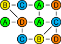
Figure 1: General coupling topology represented by a connected graph. The vertices denote the spin-$\tfrac{1}{2}$ qubits, while the edges represent pairwise couplings (e.g. of Heisenberg or Ising type). Qubits of the same colour and letter are taken to be affected by joint local unitary operations (or none if the color is white), while qubits of different kind can be controlled independently. For a system to show an outer symmetry brought about by permutations within subsets of qubits of the same type, both the graph as well as the system plus all control Hamiltonians have to remain invariant.

5 Symmetry-Constrained Controllability

A Hamiltonian quantum system is said to have a symmetry expressed by the skew-Hermitian symmetry operator $s\in\mathfrak{su}(N)$, if

$$[s,H_{\nu}]=0\quad\text{for all}\quad\nu\in\{d;1,2,\dots,m\}.$$ (10)

More precisely, we use the term outer symmetry if $s$ generates a SWAP operation permuting a subset of qubits of the same type (cp. Fig. 1) such that the coupling graph and all Hamiltonians $\{H_{\nu}\}$ are left invariant. Now subsets of qubits are termed indistinguishable if and only if they can be interchanged by an outer symmetry, i.e. a SWAP operation that is a symmetry of the system; otherwise they are distinguishable. In contrast, an inner symmetry relates to elements $s$ not generating a SWAP operation in the symmetric group of all qubit permutations.

In either case, a symmetry operator is an element of the centraliser

$$\{H_{\nu}\}^{\prime}:=\mathcal{Z}_{\mathfrak{su}(N)}(\{H_{\nu}\})=\big{\{}s\in\mathfrak{su}(N)\,|\,[s,H_{\nu}]=0\quad\forall\nu\in\{d;1,2,\dots,m\}\big{\}},$$ (11)

recalling that the centraliser of a given subset $\mathfrak{m}\subseteq\mathfrak{su}(N)$ with respect to a Lie algebra $\mathfrak{su}(N)$ consists of all elements in $\mathfrak{su}(N)$ that commute with all elements in $\mathfrak{m}$. Jacobi’s identity $\big{[}[a,b],s\big{]}+\big{[}[b,s],a\big{]}+\big{[}[s,a],b\big{]}=0$ gives two useful facts: (1) an element $s$ that commutes with the Hamiltonians $\{iH_{\nu}\}$ also commutes with their Lie closure $\mathfrak{k}$. For the dynamic Lie algebra $\mathfrak{k}$ we have

$$\mathfrak{k}^{\prime}:=\mathcal{Z}_{\mathfrak{su}(N)}(\mathfrak{k})=\{s\in\mathfrak{su}(N)\;|\;[s,k]=0\quad\forall k\in\mathfrak{k}\}$$ (12)

and hence $\{iH_{\nu}\}^{\prime}\equiv\mathfrak{k}^{\prime}$. Thus in practice it is (most) convenient to just evaluate the centraliser for a (minimal) generating set $\{iH_{\nu}\}$ of $\mathfrak{k}$ since the overall symmetry properties can be read from the local symmetries of the constituent Hamiltonians. Fact (2) means the centraliser $\mathfrak{k}^{\prime}$ forms itself an invariant Lie subalgebra (or ideal) to $\mathfrak{su}(N)$ collecting all symmetries. In summary, we obtain the following straightforward, yet important result:

Theorem 5.1.

Lack of symmetry in the sense of a trivial centraliser is a necessary condition for full controllability.

Proof 5.2.

Any non-trivial element in the centraliser would generate a one-parameter subgroup in $\mathbf{K}^{\prime}\subset\operatorname{SU}(N)$ that is not in $\mathbf{K}=\exp\mathfrak{k}$. $\hfill\blacksquare$

Algorithm 2: Determine centraliser (resp. commutant)
Algorithm 2: to system algebra $\mathfrak{k}$
	Input: Hamiltonians $I:=\{iH_{d};iH_{1},\dots,iH_{m}\}\subseteq M$
	1. For each $H\in I$ solve the homogeneous linear eqn.
	1. $\mathcal{S}_{H}:=\{s\in M|({\rm 1\negthickspace l}{}\otimes H-H^{t}\otimes{\rm 1\negthickspace l}{})\operatorname{vec}(s)=0\}$
	2. $R:=\bigcap_{H{\in}I}\mathcal{S}_{H}$.
	Output:
	Output: $R=\begin{cases}\text{centraliser $\mathfrak{k}^{\prime}$}&\text{if $M=\mathfrak{su}(N)$}\\ \text{commutant of $\mathfrak{k}$}&\text{if $M=\mathfrak{gl}(N,\mathbb{C})$}\\ \end{cases}$
	The complexity is roughly $\mathcal{O}(N^{6})$, as in Liouville space
	$N^{2}$ equations have to be solved by $LU$ decomposition.
	For $n$ qubits, $N:=2^{n}$.

Throughout this paper, we consider finite-dimensional complex matrix representations of Lie algebras, a representation being a map from a given Lie algebra to the set complex square matrices of appropriate (and finite) dimension. The matrix entries are given by complex polynomial (or equivalently holomorphic) functions. In the following, we will usually not consider the trivial representation, which maps any element to $1\in\mathbb{C}$. One particular important example for a representation of a Lie algebra is the standard representation, which is the lowest-dimensional (non-trivial) representation (with some exceptions, see the Appendix C) and which is typically used to define the corresponding Lie algebra in its matrix form. In analogy to the centraliser, one can define the commutant relative to a representation $\phi$ of dimension $\dim(\phi)$

$$\mathrm{comm}_{\phi}(\mathfrak{m}):=\big{\{}g\in\mathfrak{gl}(\dim(\phi),\mathbb{C})\,|\,[g,\phi(m)]=0\quad\forall m\in\mathfrak{m}\big{\}}$$ (13)

for a subset $\mathfrak{m}\subset\mathfrak{g}$ of a Lie algebra $\mathfrak{g}$. Now it is natural to ask how the notions of centraliser and commutant relate to irreducible representations.

Lemma 5.3.

Let $\Phi$ denote the standard representation of $\mathfrak{su}(N)$. If $\mathfrak{k}\subseteq\mathfrak{su}(N)$, then the following statements are equivalent:
(1) The centraliser $\mathfrak{k}^{\prime}=\mathcal{Z}_{\mathfrak{su}(N)}(\mathfrak{k})$ of $\mathfrak{k}$ in $\mathfrak{su}(N)$ is trivial, i.e. zero.
(2) The restriction of $\Phi$ from $\mathfrak{su}(N)$ to $\mathfrak{k}$ is irreducible.
(3) The commutant $\mathrm{comm}_{\Phi}(\mathfrak{k})$ of $\mathfrak{k}$ w.r.t. $\Phi$ is trivial, i.e. $=\{c\cdot{\rm 1\negthickspace l}{}_{N}\;|c\in\mathbb{C}\}$.

Proof 5.4.

As $\mathfrak{su}(N)$ is compact, it follows that $\Phi$ and its restriction to $\mathfrak{k}$ are completely reducible in the sense of being a direct sum of irreducible representations (see Cor. 2.17 of [65]). The representation $\Phi$ is even irreducible and faithful, i.e. injective. Hereafter, we will consider the complexification $\mathfrak{k}_{\mathbb{C}}$ of $\mathfrak{k}$ and $\mathfrak{su}(N)_{\mathbb{C}}=\mathfrak{sl}(N,\mathbb{C})$ as complexification of $\mathfrak{su}(N)$. The representation $\Phi$ has a unique extension $\Phi_{\mathbb{C}}$ to $\mathfrak{sl}(N,\mathbb{C})$, which is also irreducible and faithful. In addition, $\Phi_{\mathbb{C}}$ and its restriction to $\mathfrak{k}_{\mathbb{C}}$ are completely reducible. These facts can be deduced from Thm. 1, pp. 111–112 of [66] and Prop. 7.5 of [67].

Now it follows that (1) is equivalent to $\mathcal{Z}_{\mathfrak{sl}(N)}(\mathfrak{k}_{\mathbb{C}})=\{0\}$. As $\Phi_{\mathbb{C}}$ is faithful, this holds if and only if $\mathrm{comm}_{\Phi_{\mathbb{C}}}(\mathfrak{k}_{\mathbb{C}})$ is trivial. Relying on the fact that $\Phi_{\mathbb{C}}$ is completely reducible, $\mathrm{comm}_{\Phi_{\mathbb{C}}}(\mathfrak{k}_{\mathbb{C}})$ is trivial if and only if the restriction of $\Phi_{\mathbb{C}}$ from $\mathfrak{sl}(N,\mathbb{C})$ to $\mathfrak{k}_{\mathbb{C}}$ is irreducible. Using Thm. 1, pp. 111–112 of [66], this is equivalent to (2). As $\Phi$ is completely reducible, (2) and (3) are equivalent. $\blacksquare$

As a second consequence of a trivial centraliser the corresponding subalgebra $\mathfrak{k}$ of $\mathfrak{su}(N)$ has to be simple or semi-simple:

Lemma 5.5.

Let $\mathfrak{k}\subseteq\mathfrak{su}(N)$ be a subalgebra to the Lie algebra $\mathfrak{su}(N)$. If its centraliser $\mathfrak{k}^{\prime}$ in $\mathfrak{su}(N)$ is trivial, then $\mathfrak{k}$ is simple or semi-simple.

Proof 5.6.

By compactness, $\mathfrak{k}=\mathfrak{z}_{\mathfrak{k}}\oplus\mathfrak{s}$ decomposes into its centre $\mathfrak{z}_{\mathfrak{k}}$ and a semi-simple part $\mathfrak{s}$ (see, e.g., Cor. IV.4.25 of Ref. [67]). As the centre $\mathfrak{z}_{\mathfrak{k}}=\mathfrak{k}^{\prime}\cap\mathfrak{k}$ is trivial, $\mathfrak{k}$ can only be semi-simple or simple. $\blacksquare$

Note that the centraliser is ‘exponentially’ easier to come by than the Lie closure in the sense of comparing the asymptotic complexity $\mathcal{O}(N^{6}\cdot N^{2})$ (with $N:=2^{n}$ for $n$ qubits) of Algorithm 1 for the Lie closure with the asymptotic complexity $\mathcal{O}(N^{6})$ of Algorithm 2 for the centraliser tabulated above. — Therefore one would like to fill the gap between lack of symmetry as a necessary condition and sufficient conditions for full controllability in systems with a connected coupling topology. For pure-state controllability, this was analysed in [64], for operator controllability the issue has been raised in [25], inter alia following the lines of [68, 69], however, without a full answer. Further results in the case of pure-state controllability can be found in [39].

We have proven that the lack of symmetry is necessary for a control system to be fully controllable. Yet in turn, a control system without symmetry need not be fully controllable, as the following elementary (and pathological) example shows:

Example 5.7.

Assume we have a bilinear control system on two qubits, where the dynamic Lie algebra $\mathfrak{k}=\langle i\mathrm{XI},i\mathrm{YI},i\mathrm{ZI},i\mathrm{IX},i\mathrm{IY},i\mathrm{IZ}\rangle_{\rm Lie}=\mathfrak{su}(2)\,{\widehat{\oplus}}\,{}\mathfrak{su}(2)$ is not simple. Although it has no symmetry and its centraliser $\mathfrak{k}^{\prime}$ is in fact trivial, the system is not fully controllable: all pair terms like $i\mathrm{ZZ}$ cannot be generated, since its pathological ‘coupling graph’

is clearly not connected.

Nevertheless, the somewhat trivial example is illuminating. While in the context of $C^{*}$-algebras, von Neumann’s double-commutant theorem recovers the original algebra from the commutant of its commutant [70, 71], a similar theorem does not extend to Lie algebras [72]. Rather, if the dynamic algebra $\mathfrak{k}\subseteq\mathfrak{su}(N)$ has a trivial centraliser $\mathfrak{k}^{\prime}$, then the double centraliser $\mathfrak{k}^{\prime\prime}$, i.e. the centraliser of the centraliser in $\mathfrak{su}(N)$, of all compact semi-simple and simple irreducible proper and improper subalgebras $\mathfrak{k}$ of $\mathfrak{su}(N)$ is given by $\mathfrak{su}(N)$ in line with Lemma 5.5. However, if one considers the associative matrix algebra (with identity) generated by the basis elements (including the identity matrix) of a Lie algebra via its standard representation, then von Neumann’s double commutant theorem still holds, see Thm. (3.5.D) of Ref. [73]. — In the next step, we will thus add a criterion to single out the simple subalgebras.

Motivated by Example 5.7 one might conjecture that the dynamic algebra $\mathfrak{k}$ is simple if $\mathfrak{k}$ acts irreducibly and the coupling graph of the control system is connected. This is true for control systems in qubits with pairwise coupling interactions:

Theorem 5.8.

Consider a bilinear control system with pair interactions on $\mathfrak{su}(2^{n})$. Assume that the tensor-product structure is given by $\mathfrak{su}(2)\,{\widehat{\oplus}}\,{}\mathfrak{su}(2)\,{\widehat{\oplus}}\,{}\cdots\,{\widehat{\oplus}}\,{}\mathfrak{su}(2)$ and that the centraliser $\mathfrak{k}^{\prime}$ of the dynamic algebra $\mathfrak{k}$ is trivial. The dynamic algebra $\mathfrak{k}$ is simple if and only if the coupling graph of the control system is connected.

Proof 5.9.

See Corollary B.5(2) in Appendix B. $\blacksquare$

The general case beyond pair interactions (and qubit systems) is discussed in Appendix B. In the case of pair interactions, we say a control system is connected if its coupling graph is connected. This definition of a connected control system is a particular case of the general definition (see Appendix B) applicable to control systems which do not have a natural coupling graph.

6 Irreducible Simple Subalgebras of $\mathfrak{su}(N)$

Starting from the knowledge that for a fully controllable system the dynamic algebra $\mathfrak{k}$ has to be simple and given in an irreducible representation (see, e.g., Appendix B), it is natural to ask for a classification of all these cases. Following the work of Killing, Élie Cartan [74] classified all simple (complex) Lie algebras (see, e.g., [75, 76]). The corresponding compact real forms ([76, 77]) are the compact simple Lie algebras of classical type (assuming $\ell\in\mathbb{N}{}\setminus\{0\}$ henceforth):

$$\mathfrak{a}_{\ell}: \quad\mathfrak{su}(\ell+1),$$

$$\mathfrak{b}_{\ell}: \quad\mathfrak{so}(2\ell+1),$$

$$\mathfrak{c}_{\ell}: \quad\mathfrak{sp}(\ell):=\mathfrak{sp}(2\ell,\mathbb{C})\cap\mathfrak{u}(2\ell,\mathbb{C}),$$

$$\mathfrak{d}_{\ell}: \quad\mathfrak{so}(2\ell),$$

and of exceptional type $\mathfrak{e}_{6}$, $\mathfrak{e}_{7}$, $\mathfrak{e}_{8}$, $\mathfrak{f}_{4}$, $\mathfrak{g}_{2}$. Note also that for $\mathfrak{a}_{\ell}$ ($\ell\geq 1$), $\mathfrak{b}_{\ell}$ ($\ell\geq 2$), $\mathfrak{c}_{\ell}$ ($\ell\geq 3$) and $\mathfrak{d}_{\ell}$ ($\ell\geq 4$) the following isomorphisms (see, e.g., Thm. X.3.12 in [77]) $\mathfrak{su}(2)\cong\mathfrak{so}(3)\cong\mathfrak{sp}(1)$, $\mathfrak{so}(5)\cong\mathfrak{sp}(2)$, and $\mathfrak{su}(4)\cong\mathfrak{so}(6)$ are no longer of concern. The same holds for the abelian case $\mathfrak{so}(2)$ as well as for the semi-simple one $\mathfrak{so}(4)\cong\mathfrak{su}(2)\,{\widehat{\oplus}}\,{}\mathfrak{su}(2)$.

Pro memoria. The classical, compact simple Lie algebras and some forms of their standard matrix representations may be given as follows:

algebra	definition and block forms		Lie dimension
$\mathfrak{su}(N):=\{a\in\mathbb{C}^{N\times N}\;|\;a^{\dagger}=-a,\;\operatorname{tr}a=0\}$			$N^{2}-1$
$\mathfrak{so}(N):=\{a=U\tilde{a}U^{\dagger}\in\mathbb{C}^{N\times N}\;|\;\tilde{a}^{t}=-\tilde{a},\;\operatorname{tr}\tilde{a}=0\}$			$\tfrac{1}{2}N(N-1)$
	with $U\in SU(N)$
$N=2\ell$:	$a^{\prime}=\begin{pmatrix}A&\phantom{-}B\phantom{{}^{t}}\\ C&-A^{t}\end{pmatrix}\;$
	with $A,B,C\in\mathbb{C}^{\ell\times\ell},B^{t}=-B,C^{t}=-C$
$N=2\ell+1$:	$a^{\prime}=\begin{pmatrix}A&\phantom{-}B\phantom{{}^{t}}&u\\ C&-A^{t}&v\\ -u^{t}&-v^{t}&0\end{pmatrix}\;$
	with $A,B,C\;\text{as above and}\;u,v\in\mathbb{C}^{\ell}$
NB: the representations $\tilde{a}$ and $a^{\prime}$ above need not be equal.
$\mathfrak{sp}(N/2):=\{a=U\tilde{a}U^{\dagger}\in\mathbb{C}^{N\times N}\;|\;J\tilde{a}=-\tilde{a}^{t}J\}$			$\tfrac{1}{2}N(N+1)$
	with $J:=\left(\begin{smallmatrix}0\phantom{{}_{\ell}}&-{\rm 1\negthickspace l}{}_{\ell}\\ {\rm 1\negthickspace l}{}_{\ell}&\phantom{-}0\phantom{{}_{\ell}}\end{smallmatrix}\right),U\in SU(N)$
$N=2\ell$:	$\tilde{a}=\begin{pmatrix}A&\phantom{-}B\phantom{{}^{t}}\\ C&-A^{t}\end{pmatrix}$
	with $A,B,C\in\mathbb{C}^{\ell\times\ell},B=B^{t},C=C^{t}$

By completeness of Cartan’s classification above we may summarise as follows:

Corollary 6.1 (Candidate List).

Consider a bilinear control system, where the drift and control Hamiltonians $\{iH_{\nu}\}$ generate the dynamic system Lie algebra $\mathfrak{k}\subseteq\mathfrak{su}(N)$ in an irreducible representation ($\mathfrak{k}^{\prime}$ trivial) with the additional promise that $\mathfrak{k}$ is simple (e.g. due to a connected control system). Then, being a simple subalgebra of $\mathfrak{su}(N)$, the system algebra $\mathfrak{k}$ has to be one of the candidate compact simple Lie algebras: $\mathfrak{su}(\ell+1)$, $\mathfrak{so}(2\ell+1)$, $\mathfrak{sp}(\ell)$, $\mathfrak{so}(2\ell)$, $\mathfrak{e}_{6}$, $\mathfrak{e}_{7}$, $\mathfrak{e}_{8}$, $\mathfrak{f}_{4}$, or $\mathfrak{g}_{2}$. $\blacksquare$

For illustration of the Lie algebras of exceptional type, consider the dimensions of their standard representations (see, e.g., p. 218 of Ref. [76], Ref. [79], Ref. [80]) $\mathfrak{e}_{6}\subset\mathfrak{su}(27)$, $\mathfrak{e}_{7}\subset\mathfrak{sp}(28)$, $\mathfrak{e}_{8}\subset\mathfrak{so}(248)$, $\mathfrak{f}_{4}\subset\mathfrak{so}(26)$, and $\mathfrak{g}_{2}\subset\mathfrak{so}(7)$. As a final remark on exceptional Lie algebras suffice it to add that—with the single exception of $\mathfrak{g}_{2}$—they all fail to generate groups acting transitively on the sphere or on $\mathbb{R}^{N}\setminus\{0\}$. This has been shown in [81] building upon results in [82] to fill gaps in earlier work [83, 84].

Having listed all the candidates for proper simple subalgebras of $\mathfrak{su}(N)$, we now focus on the set of possible irreducible representations. To this end, in this chapter we describe the main results, while all the details shall be explained in the Appendix C. The irreducible representations of simple (complex) Lie algebras were already determined by Élie Cartan [85]. This classification is equivalent for the compact simple Lie algebras (or the compact connected simple Lie groups), see, e.g., [76]. The irreducible simple subalgebras of $\mathfrak{su}(N)$ are found by enumerating for all simple Lie algebras all their irreducible representations of dimension $N$. The dimensions of the irreducible representations can be efficiently computed using computer algebra systems such as LiE [86] and MAGMA [87] via Weyl’s dimension formula. Following the work of Dynkin [88] (see App. C.3 and Chap. 6, Sec. 3.2 of Ref. [90]), one can determine the inclusion relations between irreducible simple subalgebras of $\mathfrak{su}(N)$. We obtained all the irreducible simple subalgebras of $\mathfrak{su}(N)$ for $N\leq 2^{15}=32768$. This significantly extends previous work [38, 39] for $N\leq 9$. The results for $N\leq 16$ are given in Tab. 1, those for $N=2^{n}$ and $1\leq n\leq 15$ are relegated to Tab. 2. A complete list with all the results for $N\leq 2^{15}$ is attached as Supplementary Material [91].

Table 1: The Irreducible Simple Subalgebras of $\mathfrak{su}(N)$ for $N\leq 16$

NB: $\mathfrak{so}(3)\cong\mathfrak{su}(2)\cong\mathfrak{sp}(1)$, $\mathfrak{so}(5)\cong\mathfrak{sp}(2)$, and $\mathfrak{so}(6)\cong\mathfrak{su}(4)$.

Remark 6.2.

With regard to Tables 1 and 2, the occurrence of $\mathfrak{su}(2)$ as an irreducible simple subalgebra to any $\mathfrak{su}(N)$ with $N\geq 2$ is natural from the point of view of spin physics. We identify $\mathfrak{su}(N)=\mathfrak{su}(2j+1)$, where the (non-vanishing) half-integer and integer spin-quantum numbers may take the values $j\in\{\tfrac{1}{2},1,\tfrac{3}{2},2,\dots\}$. Now to any such $j$ there is an irreducible spin-$j$ representation of the three Pauli matrices generating $\mathfrak{su}(2)$. For instance, in $\mathfrak{su}(4)$ there is an irreducible spin-$\tfrac{3}{2}$ representation of $\mathfrak{su}(2)$ as a proper irreducible subalgebra ${\mathfrak{su}(2)}\subsetneq\mathfrak{su}(4)$. — In contrast, the Gell-Mann basis to $\mathfrak{su}(2j+1)$ comprises a reducible representation of $\mathfrak{su}(2)$ as a subalgebra. Clearly, the two types of representations are inequivalent.

Table 2: The Irreducible Simple Subalgebras of $\mathfrak{su}(2^{n})$ for $1\leq n\leq 15$

In the set of irreducible simple subalgebras of $\mathfrak{su}(N)$, the subalgebras $\mathfrak{sp}(N/2)$ with $N$ even and $\mathfrak{so}(N)$ play a particularly important role. For $N\geq 5$, we discuss the irreducible simple subalgebras of $\mathfrak{su}(N)$ for $N$ even and odd. If $N\geq 5$ is even, then $\mathfrak{su}(N)$ has both $\mathfrak{sp}(N/2)$ and $\mathfrak{so}(N)$ as irreducible simple subalgebras. In addition, $\mathfrak{su}(2)\subset\mathfrak{sp}(N/2)$ occurs as irreducible simple subalgebra. We consider two types of trivial cass. First, if $N\geq 5$ is even and if $\mathfrak{sp}(N/2)$, $\mathfrak{so}(N)$, and $\mathfrak{su}(2)\subset\mathfrak{sp}(N/2)$ are the only proper irreducible simple subalgebras, then we say the case is trivial. A trivial example is given by $\mathfrak{su}(12)$ in Tab. 1. If $N\geq 5$ is odd, then $\mathfrak{so}(N)$ is an irreducible simple subalgebra of $\mathfrak{su}(N)$ but $\mathfrak{sp}(N/2)$ is not (as $N/2$ is not an integer). Moreover, $\mathfrak{su}(2)\subset\mathfrak{so}(N)$ occurs as irreducible simple subalgebra. Second, if $N\geq 5$ is odd and if $\mathfrak{so}(N)$ as well as $\mathfrak{su}(2)\subset\mathfrak{so}(N)$ are the only proper irreducible simple subalgebras, then we say the case is trivial. Examples of such trivial cases are given by $\mathfrak{su}(5)$, $\mathfrak{su}(9)$, $\mathfrak{su}(11)$, and $\mathfrak{su}(13)$ in Tab. 1. The irreducible subalgebras $\mathfrak{sp}(N/2)$ and $\mathfrak{so}(N)$ correspond to the symmetric spaces $\mathrm{SU}(N)/\mathrm{Sp}(N/2)$ and $\mathrm{SU}(N)/\mathrm{SO}(N)$. These are two of three possible symmetric spaces [77] of $\mathrm{SU}(N)$, where the third type does not correspond to a semi-simple subalgebra of $\mathfrak{su}(N)$.

We call a representation $\phi$ of a subalgebra $\mathfrak{k}$ symplectic [orthogonal] if the subalgebra $\mathfrak{k}$ given in the representation $\phi$ is conjugate to a subalgebra of $\mathfrak{sp}(N/2)$ [$\mathfrak{so}(N)$]. If the representation is neither symplectic nor orthogonal, we term it unitary. In abuse of notation, we call also the subalgebra $\mathfrak{k}$ (w.r.t. some fixed but unspecified representation $\phi$) symplectic, orthogonal, or unitary, if the respective representation $\phi$ is symplectic, orthogonal, or unitary. We emphasise that the classification of a subalgebra depends on the representations considered, see also Chap. IX, App. II.2, Prop. 3 of Ref. [76].

The property of a representation to be symplectic [resp. orthogonal] corresponds to the existence of an invariant (non-degenerate) skew-symmetric [resp. symmetric] bilinear form on the space of the representation. For irreducible representations in the compact case [e.g. for subgroups of $\operatorname{SU}(N)$], this correspondence is an equivalence and a proof can be found in Sec. 3.11, Thm. H of Ref. [93]. As an invariant (non-degenerate) bilinear form can either be skew-symmetric or symmetric, it follows that the same holds for the classification of (irreducible) symplectic, orthogonal, or unitary representations (Chap. IX, Sec. 7.2, Prop. 1 of Ref. [76]):

Lemma 6.3.

An irreducible representation $\phi(\mathfrak{k})$ can either be symplectic, or orthogonal, or unitary.

7 From Necessary to Sufficient Conditions for Controllability

While the ramification of mathematically admissible irreducible simple candidate subalgebras may seem daunting, in the following we will eliminate candidates by simple means. More precisely, we arrive at the following.

Corollary 7.1 (Task List).

One way of showing full controllability amounts to excluding other candidates of irreducible simple subalgebras, which can be
(1) symplectic, i.e. conjugate to a subalgebra of $\mathfrak{sp}(N/2)$,
(2) orthogonal, i.e. conjugate to a subalgebra of $\mathfrak{so}(N)$,
(3) or unitary in the remaining cases.
In particular, one has to exclude cases like the exceptional ones $\mathfrak{e}_{6}$, $\mathfrak{e}_{7}$, $\mathfrak{e}_{8}$ $\mathfrak{f}_{4}$, $\mathfrak{g}_{2}$. The unitary, irreducible simple subalgebras can occur in the cases $\mathfrak{su}(\ell+1)\subsetneq\mathfrak{su}(N)$ ($\ell\geq 2$), $\mathfrak{so}(4\ell+2)$, and $\mathfrak{e}_{6}$. $\hfill\blacksquare$

In what follows, the plan is to make use of the fact that in Tabs. 1 and 2, most of the irreducible subalgebras are symplectic or orthogonal. The symplectic and orthogonal ones (including their nested subalgebras!) will be excluded by merely solving simultaneous systems of linear homogeneous equations, which will also exclude the exceptional algebras $\mathfrak{e}_{7}$, $\mathfrak{e}_{8}$, $\mathfrak{f}_{4}$, and $\mathfrak{g}_{2}$, just leaving $\mathfrak{e}_{6}$. It appears that for systems of dimension $2^{n}$, irreducible representations of $\mathfrak{e}_{6}$ cannot be an irreducible simple subalgebra of $\mathfrak{su}(2^{n})$ without being a subalgebra to an intermediate orthogonal or symplectic algebra.

In principle, the task of identifying the dynamic Lie algebra can also be solved by algorithms [94, 95] available in the computer algebra system MAGMA [87]. Yet, here we focus on exploiting algorithms that are more efficient, since they boil down to solving systems of homogeneous linear equations, which currently can—in general—be carried to matrix sizes of about $6\cdot 10^{4}\times 6\cdot 10^{4}$ (and in extreme cases to $10^{5}\times 10^{5}$)[96]. So the algorithms presented here aim at the more specific task of distinguishing $\mathfrak{su}(N)$ from its proper irreducible simple subalgebras, a task our algorithms are more efficient in.

7.1 Symplectic and Orthogonal Subalgebras

In order to decide on conjugation to irreducible subalgebras which are symplectic and orthogonal, we need more detail. To this end, recalling the following Lemma will prove useful to apply the lines of [99] in streamlined form leading to an explicit algorithm.

Lemma 7.2.

(1) Every unitary symmetric matrix $S=S^{t}\in U(N,\mathbb{C})$ is unitarily $t$-congruent to the identity, i.e. $S=T^{t}{\rm 1\negthickspace l}{}\,T$ with $T$ unitary.
(2) Every unitary skew-symmetric matrix $S=-S^{t}\in U(N,\mathbb{C})$ with $N$ even is unitarily $t$-congruent to $J$, i.e. $S=T^{t}JT$ with $T$ unitary and

$$J:=\begin{pmatrix}0&-{\rm 1\negthickspace l}{}_{N/2}\\ {\rm 1\negthickspace l}{}_{N/2}&0\end{pmatrix}.$$ (14)

Proof 7.3.

(1) Follows by singular-value decomposition and goes back to Hua ([100], Thm. 5). (2) Follows likewise from the same source (ibid., Thm. 7). $\blacksquare$

Lemma 7.4.

Suppose $\mathfrak{k}\subset\mathfrak{su}(N)$ is simple and $J$ is defined as in Eqn. (14). Then the element $iH\in\mathfrak{k}$
(1) is unitarily conjugate to $i\widetilde{H}\in\mathfrak{so}(N)$, where $\widetilde{H}^{t}=-\widetilde{H}$, if and only if there exists a symmetric unitary $S$ (so $S\bar{S}=+{\rm 1\negthickspace l}{}_{N}$) satisfying $SH+H^{t}S=0$;
(2) is unitarily conjugate to $i\widetilde{H}\in\mathfrak{sp}({N}/{2})$ (with $N$ even), where $J\widetilde{H}=-\widetilde{H}^{t}J$, if and only if there is a skew-symmetric unitary $S$ (so $S\bar{S}=-{\rm 1\negthickspace l}{}_{N}$) satisfying $SH+H^{t}S=0$.

Proof 7.5.

First observe that whenever there is a unitary $T$ such that $THT^{\dagger}=:\widetilde{H}$ with $L\widetilde{H}=-\widetilde{H}^{t}L$, this is equivalent to

$$LTHT^{\dagger}=-(THT^{\dagger})^{t}L\Leftrightarrow LTH=-\bar{T}H^{t}T^{t}LT\Leftrightarrow(\underbrace{T^{t}LT}_{S})H=-H^{t}(\underbrace{T^{t}LT}_{S}).$$

Now it is easy to establish that the conditions are sufficient (“$\Rightarrow$”):
(1) Setting $L:={\rm 1\negthickspace l}{}_{N}$ and $S:=T^{t}T$ gives $S\bar{S}=T^{t}TT^{\dagger}\bar{T}=+{\rm 1\negthickspace l}{}_{N}$. Thus $S=S^{t}$ is unitary, complex symmetric and satifies $SH=-H^{t}S$.
(2) Setting $L:=J$ and $S:=T^{t}JT$ gives $S\bar{S}=T^{t}JTT^{\dagger}J\bar{T}=-{\rm 1\negthickspace l}{}_{N}$ by $J^{2}=-{\rm 1\negthickspace l}{}_{N}$. Thus $S=-S^{t}$ is unitary, skew-symmetric and satifies $SH=-H^{t}S$.

Moreover the conditions are also necessary (“$\Leftarrow$”) by Lemma 7.2, because with appropriate respective unitaries $T$
(1) for $L={\rm 1\negthickspace l}{}_{N}$ any symmetric unitary matrix $S$ can be written as $S=T^{t}T$;
(2) for $L=J$ any skew-symmetric unitary matrix $S$ can be written as $S=T^{t}JT$.
XX   $\blacksquare$

Algorithm 3: Check conjugation to subalgebras of $\mathfrak{so}(N)$ or $\mathfrak{sp}(N/2)$
	Input: Hamiltonians $I:=\{iH_{d};iH_{1},\dots,iH_{m}\}\subseteq\mathfrak{su}(N)$
	1. For each Hamiltonian $H\in I$ determine all non-singular
	1. solutions to the homogeneous linear equation
	1. $\mathcal{S}_{H}:=\{S\in SL(N)|SH+H^{t}S=0\}$
	1. $\mathcal{S}_{H}:$$=\{S\in SL(N)|(H^{t}\otimes{\rm 1\negthickspace l}{}+{\rm 1\negthickspace l}{}\otimes H^{t})\operatorname{vec(S)}=0\}$
	2. $\mathcal{S}:=\bigcap_{H{\in}I}\mathcal{S}_{H}$
	Output: (a) $\exists S\in\mathcal{S}\text{ s.t.\ }S\bar{S}=+{\rm 1\negthickspace l}{}$ $\Leftrightarrow$ $\mathfrak{k}\subseteq\mathfrak{so}(N)$
	Output: (b) $\exists S\in\mathcal{S}\text{ s.t.\ }S\bar{S}=-{\rm 1\negthickspace l}{}$ $\Leftrightarrow$ $\mathfrak{k}\subseteq\mathfrak{sp}(N/2)$
	Output: (c)  $\nexists S\in\mathcal{S}$ $\Rightarrow$ $\mathfrak{k}\not\subseteq\mathfrak{so}(N)$ and $\mathfrak{k}\not\subseteq\mathfrak{sp}(N/2)$
	Output: The cases (a) and (b) are mutually exclusive
	Output: if the centraliser of $I$ is trivial.
	The complexity is roughly $\mathcal{O}(N^{6})$, as in Liouville space
	$N^{2}$ equations have to be solved by $LU$ decomposition ($N:=2^{n}$).

In the context of filtering simple subalgebras, Lemma 7.4 can be turned into the powerful Algorithm 3. It boils down to checking a system of homogeneous linear equations for solutions $S$ satisfying $SH_{\nu}=-H_{\nu}^{t}S$ for all $iH_{\nu}\in\mathfrak{k}$ simultaneously: if $S$ is a solution with $S\bar{S}=+{\rm 1\negthickspace l}{}$, the subalgebra $\mathfrak{k}$ of $\mathfrak{su}(N)$ generated by the $\{iH_{\nu}\}$ is conjugate to a subalgebra of $\mathfrak{so}(N)$, while in case of $S\bar{S}=-{\rm 1\negthickspace l}{}$, $\mathfrak{k}$ is conjugate to a subalgebra of $\mathfrak{sp}({N}/{2})$.

Remark 7.6.

By irreducibility of $\mathfrak{k}$ (via Algorithm 2), those subgroups generated by $\mathfrak{k}\subset\mathfrak{su}(2^{n})$ with a unitary representation equivalent to its complex conjugate are limited to orthogonal and symplectic ones: it follows from Schur’s Lemma that $S\bar{S}=\pm{\rm 1\negthickspace l}{}$ are in fact the only types of solutions for $SH=-H^{t}S$ with $iH\in\mathfrak{k}$, as nicely explained in Lem. 3 of Ref. [99]. Lemma 6.3 (of this paper) explains why these solutions are mutually exclusive. Due to the irreducibility, the matrix $S$ is unique up to a scalar factor $c\in\mathbb{C}$ with $c\bar{c}=1$.

Conjugation to the symplectic algebras has also been treated in Ref. [84] by solving a system of linear equations, while Ref. [101] resorted to determining eigenvalues for discerning the unitary case from conjugate symplectic or orthogonal subalgebras. — The results can be summarised and extended as follows:

Theorem 7.7 (Candidate Filter I).

Consider a set of Hamiltonians $\{iH_{\nu}\}$ generating the dynamic algebra $\mathfrak{k}\subseteq\mathfrak{su}(N)$ with the promise (by Algorithm 2 and e.g. due to a connected control system) that $\mathfrak{k}\subseteq\mathfrak{su}(N)$ is given in an irreducible representation and $\mathfrak{k}$ is simple. If in addition Algorithm 3 has but an empty set of solutions, then $\mathfrak{k}$ is neither conjugate to a simple subalgebra of $\mathfrak{sp}({N}/{2})$ nor of $\mathfrak{so}(N)$. In particular, $\mathfrak{k}$ is none of the following simple Lie algebras: $\mathfrak{e}_{7}$, $\mathfrak{e}_{8}$, $\mathfrak{f}_{4}$, or $\mathfrak{g}_{2}$.

Proof 7.8.

The cases $\mathfrak{so}(N)$ and $\mathfrak{sp}(N)$ are settled by Lemma 7.4. The cases $\mathfrak{e}_{7}$, $\mathfrak{e}_{8}$, $\mathfrak{f}_{4}$, and $\mathfrak{g}_{2}$ follow from the elaborate classification of Malcev [92] (see also, e.g., [88, 102, 38] and Theorem C.10 in Appendix C.3), as an irreducible representation of $\mathfrak{e}_{8}$, $\mathfrak{f}_{4}$, or $\mathfrak{g}_{2}$ is always conjugate to a subalgebra of $\mathfrak{so}(N)$, while an irreducible representation of $\mathfrak{e}_{7}$ is conjugate either to a subalgebra of $\mathfrak{so}(N)$ or of $\mathfrak{sp}(N/2)$. $\blacksquare$

7.2 Unitary Subalgebras

It also follows from Malcev [92] (again, see also [88, 102, 38] and Theorem C.10 in Appendix C.3) that only the subalgebras $\mathfrak{su}(\ell+1)$ ($\ell\geq 2$), $\mathfrak{so}(4\ell+2)$, and $\mathfrak{e}_{6}$ can have unitary representations. One can immediately deduce from the Tables 1 and 2 the following

Corollary 7.9.

The Lie algebras $\mathfrak{su}(2^{n})$ do not possess (proper) unitary, irreducible simple subalgebras if $n\in\{1,2,3,5,7,9,11,13,15\}$. In these cases ($n\neq 1$) and under the conditions of Theorem 7.7, Algorithm 3 provides a necessary and sufficient criterion for full controllability. $\blacksquare$

We checked by explicit computations that $\mathfrak{e}_{6}$ does not occur as a unitary, irreducible simple subalgebra of $\mathfrak{su}(2^{n})$ for $n\leq 100$, i.e. for qubit systems with up to $100$ qubits. Thus one might conjecture that $\mathfrak{e}_{6}$ does not occur as a unitary, irreducible simple subalgebra for qubit systems in general.

We present an example of a control system whose dynamic algebra is a (proper) unitary subalgebra of $\mathfrak{su}(2^{4})$:

Example 7.10.

Consider a bilinear control system on $\mathfrak{su}(16)$ with four subsystems given by $\mathfrak{su}(2)\,{\widehat{\oplus}}\,{}\mathfrak{su}(2)\,{\widehat{\oplus}}\,{}\mathfrak{su}(2)\,{\widehat{\oplus}}\,{}\mathfrak{su}(2)$. The local dynamic algebra is given by

$$\langle i\mathrm{XIII},i\mathrm{YIII},i\mathrm{ZIII},i\mathrm{IIIX},i\mathrm{IIIY},i\mathrm{IIIZ}\rangle_{\rm Lie}.$$

In addition, we have a drift Hamiltonian $H_{d}=\mathrm{XXII}+\mathrm{YYII}+\mathrm{IXXI}+\mathrm{IYYI}+\mathrm{IIXX}+\mathrm{IIYY}$ (Heisenberg-XX interaction). The control system

is connected and acts irreducibly. The dynamic algebra $\mathfrak{k}=\mathfrak{so}(10)$ is simple and a (proper) unitary subalgebra of $\mathfrak{su}(16)$.

7.3 System Algebras Comprising Local Actions $\mathfrak{su}(2)^{\oplus n}$

We now discuss the set of local unitary transformations $\mathrm{SU}(2)^{\otimes n}\subseteq\mathrm{SU}(2^{n})$ and its Lie algebra $\mathfrak{su}(2)^{\oplus n}\subseteq\mathfrak{su}(2^{n})$ where both are given in their respective standard representation, i.e. as $n$-fold Kronecker product and $n$-fold Kronecker sum (see Sec. 4)

$$\mathfrak{su}(2)\,{\widehat{\oplus}}\,{}\mathfrak{su}(2)\,{\widehat{\oplus}}\,{}\cdots\,{\widehat{\oplus}}\,{}\mathfrak{su}(2).$$

What is the classification of $\mathfrak{su}(2)^{\oplus n}$ w.r.t. symplectic, orthogonal, and unitary subalgebras? We obtain from Thm. 3 of Ref. [11] (see also [103, 104]):

Lemma 7.11.

For the algebra $\mathfrak{su}(2)^{\oplus n}$ given in its (irreducible) standard representation there are two cases: (1) if $n$ is odd, it is a symplectic subalgebra of $\mathfrak{su}(2^{n})$ in the sense of being conjugate to a subalgebra of $\mathfrak{sp}(2^{n-1})$, and (2) if $n$ is even, it is an orthogonal subalgebra in the sense of being conjugate to a subalgebra of $\mathfrak{so}(2^{n})$.

Proof 7.12.

Let $\phi$ denote an irreducible representation of a compact Lie group $\mathrm{G}$. Then for the Frobenius-Schur indicator (Chap. IX, App. II.2, Prop. 4 of Ref. [76]) one finds

$$\int_{G}\mathrm{Tr}[\phi^{2}(g)]\;dg=\begin{cases}-1&\Leftrightarrow\quad\text{$\phi$ is a {\em symplectic} representation}\\ +1&\Leftrightarrow\quad\text{$\phi$ is an {\em orthogonal} representation}\\ \phantom{+}0&\Leftrightarrow\quad\text{$\phi$ is a {\em unitary} representation}\\ \end{cases}$$

Let $\psi$ denote the standard representation of the Lie group $\mathrm{H}=\operatorname{SU}(2)^{\otimes n}$. Ref. [11] proves that $\int_{H}\mathrm{Tr}[\psi^{2}(h)]\;dh=(-1)^{n}$. $\blacksquare$

If the subsystems of a control system are independently fully controllable then it follows from Lemma 7.11 that some cases can be excluded:

Lemma 7.13.

Assume that the dynamic algebra $\mathfrak{k}\subseteq\mathfrak{su}(2^{n})$ is irreducible and simple, and that the subsystems $\mathfrak{su}(2)$ are independently fully controllable [i.e. $\mathfrak{k}\supseteq\mathfrak{su}(2)\,{\widehat{\oplus}}\,{}\mathfrak{su}(2)\,{\widehat{\oplus}}\,{}\cdots\,{\widehat{\oplus}}\,{}\mathfrak{su}(2)$]. If $n$ is odd [resp. even] then $\mathfrak{k}$ is not an orthogonal [resp. symplectic] subalgebra.

Proof 7.14.

We remark that $\mathfrak{h}=\mathfrak{su}(2)\,{\widehat{\oplus}}\,{}\mathfrak{su}(2)\,{\widehat{\oplus}}\,{}\cdots\,{\widehat{\oplus}}\,{}\mathfrak{su}(2)$ is given in an irreducible representation. It follows from the discussion prior to Lemma 6.3 that $\mathfrak{h}$ has an invariant (non-degenerate) skew-symmetric bilinear form and no invariant (non-degenerate) symmetric bilinear form if $n$ is odd. Therefore, the dynamic algebra $\mathfrak{k}$ cannot have an invariant (non-degenerate) symmetric bilinear form and the Lemma follows for odd $n$. The case of even $n$ is similar. $\blacksquare$

Unfortunately, Lemma 7.13 is no longer true if the dynamic algebra contains only a non-zero subset of the local operations:

Example 7.15.

Consider a bilinear control system on $\mathfrak{su}(8)$ with three subsystems given by $\mathfrak{su}(2)\,{\widehat{\oplus}}\,{}\mathfrak{su}(2)\,{\widehat{\oplus}}\,{}\mathfrak{su}(2)$. The local dynamic algebra is $\langle i\mathrm{XII},i\mathrm{YII},i\mathrm{ZII}\rangle_{\rm Lie}$. In addition, we have a drift Hamiltonian $H_{d}=\mathrm{XXI}+\mathrm{YYI}+\mathrm{IXX}+\mathrm{IYY}$. The control system

is connected and acts irreducibly. The dynamic algebra $\mathfrak{k}=\mathfrak{so}(7)$ is simple and an orthogonal subalgebra. We emphasise that as a consequence of Lemma 7.13 this would have not been possible if $\mathfrak{k}\supseteq\mathfrak{su}(2)\,{\widehat{\oplus}}\,{}\mathfrak{su}(2)\,{\widehat{\oplus}}\,{}\mathfrak{su}(2)$.

7.4 A Necessary and Sufficient Symmetry Condition

In this subsection we present a necessary and sufficient symmetry criterion for full controllability of control systems contained in $\mathfrak{su}(N)$. To this end, we introduce some additional notation: Assume that $\phi$ is a representation of a compact Lie algebra of dimension $N$. The tensor square $\phi^{\otimes 2}:=\phi\otimes{\rm 1\negthickspace l}{}_{N}+{\rm 1\negthickspace l}{}_{N}\otimes\phi$ decomposes as $\phi^{\otimes 2}=\mathrm{Alt}^{2}\phi\oplus\mathrm{Sym}^{2}\phi$, where the alternating square $\mathrm{Alt}^{2}\phi$ and the symmetric square $\mathrm{Sym}^{2}\phi$ are the restrictions of $\phi^{\otimes 2}$ to the antisymmetric and the symmetric subspace, respectively. More details on this notation is given in Appendix D. We arrive at

Theorem 7.16.

Assume that $\mathfrak{k}$ is a subalgebra of $\mathfrak{su}(N)$ and denote by $\Phi$ the standard representation of $\mathfrak{su}(N)$. Then, the following are equivalent:
(1) $\mathfrak{k}=\mathfrak{su}(N)$.
(2) The restrictions of $\mathrm{Alt}^{2}\Phi$ and $\mathrm{Sym}^{2}\Phi$ to the subalgebra $\mathfrak{k}$ are both irreducible.
(3) The commutant $\mathrm{comm}_{\Phi^{\otimes 2}}(\mathfrak{k})$ w.r.t. the tensor square $\Phi^{\otimes 2}$ has dimension two.

Proof 7.17.

(1) $\Rightarrow$ (2) follows by Theorem D.3 in Appendix D. We prove (2) $\Rightarrow$ (1). As the restriction $(\mathrm{Alt}^{2}\Phi)|_{\mathfrak{k}}$ of $\mathrm{Alt}^{2}\Phi$ to $\mathfrak{k}$ is irreducible, we get that the restriction $\Phi|_{\mathfrak{k}}$ of $\Phi$ to $\mathfrak{k}$ is also irreducible. Otherwise, $\Phi|_{\mathfrak{k}}=\phi_{1}\oplus\phi_{2}$ would be reducible and, as a consequence, $(\mathrm{Alt}^{2}\Phi)|_{\mathfrak{k}}=\mathrm{Alt}^{2}(\phi_{1}\oplus\phi_{2})=\mathrm{Alt}^{2}\phi_{1}\oplus(\phi_{1}\otimes\phi_{2})\oplus\mathrm{Alt}^{2}\phi_{2}$ would also be reducible (which is impossible). Lemma 5.3 implies the centraliser $\mathfrak{k}^{\prime}$ of $\mathfrak{k}$ in $\mathfrak{su}(N)$ is trivial, thus by Lemma 5.5 $\mathfrak{k}$ is semisimple. Now (1) follows by Theorem D.3 in Appendix D. Moreover Thm. 1.5 of Ref. [105] says that the dimension of the commutant of a representation $\phi$ is given by $\sum_{i}m_{i}^{2}$ where the $m_{i}$ are the multiplicities of the irreducible components of $\phi$. As we consider the representation $(\Phi^{\otimes 2})|_{\mathfrak{k}}=(\mathrm{Alt}^{2}\Phi)|_{\mathfrak{k}}\oplus(\mathrm{Sym}^{2}\Phi)|_{\mathfrak{k}}$, the equivalence of (2) and (3) readily follows. $\blacksquare$

We now show that condition (3) of Theorem 7.16 can be easily tested using a set of Hamiltonians $\{iH_{\nu}\}$ generating the dynamic algebra $\mathfrak{k}\subseteq\mathfrak{su}(N)$. Therefore, we prove that the commutant of $\{(iH_{\nu})\otimes{\rm 1\negthickspace l}{}_{N}+{\rm 1\negthickspace l}{}_{N}\otimes(iH_{\nu})\}$ is equal to $\mathrm{comm}_{\Phi^{\otimes 2}}(\mathfrak{k})$. Obviously, the latter commutant is contained in the former. Let $s\in\mathfrak{gl}(N^{2},\mathbb{C})$ be an element of the former commutant. Then by Jacobi’s identity $\big{[}[a,b],s\big{]}+\big{[}[b,s],a\big{]}+\big{[}[s,a],b\big{]}=0$, $s$ commutes with all commutators

$$[(iH_{\nu})\otimes{\rm 1\negthickspace l}{}_{N}+{\rm 1\negthickspace l}{}_{N}\otimes(iH_{\nu}),(iH_{\mu})\otimes{\rm 1\negthickspace l}{}_{N}+{\rm 1\negthickspace l}{}_{N}\otimes(iH_{\mu})]$$

$$=[iH_{\nu},iH_{\mu}]\otimes{\rm 1\negthickspace l}{}_{N}+{\rm 1\negthickspace l}{}_{N}\otimes[iH_{\nu},iH_{\mu}],$$

and by induction, $s$ is also contained in the latter commutant.

Together with Theorem 7.16, we thus obtain a necessary and sufficient symmetry condition for full controllability as a theoretical main result:

Corollary 7.18.

Consider a set of Hamiltonians $\{iH_{\nu}\,|\,\nu=d,1,2,\dots\}$ generating the dynamic algebra $\mathfrak{k}\subseteq\mathfrak{su}(N)$. The corresponding control system is fully controllable in the sense $\mathfrak{k}=\mathfrak{su}(N)$, if and only if the joint commutant of $\{(iH_{\nu})\otimes{\rm 1\negthickspace l}{}_{N}+{\rm 1\negthickspace l}{}_{N}\otimes(iH_{\nu})\,|\,\nu=d,1,2,\dots\}$ has dimension two. $\blacksquare$

In spite of the beauty of simplicity of this result, from an algorithmic point of view the above symmetry condition is currently not appealing: In Corollary 7.18 one would have to compute the commutant of $N^{2}\times N^{2}$ matrices as compared to $N\times N$ matrices in the test for the lack of symmetry in Algorithm 2. Thus the complexity of testing for Corollary 7.18 would be the square of the complexity of Algorithm 2. Even in moderately-sized examples one has to save computer memory by methods of sparse matrices due to the larger matrices. In larger examples, testing for Corollary 7.18 gets impractical. Yet compared with potential conditions involving even higher tensor powers, one should consider Corollary 7.18 as a fortunate incidence.

In order to characterise the commutant of Corollary 7.18 in further detail, we introduce an $N^{2}\times N^{2}$ permutation matrix $K_{N,N}$ also known as commutation matrix [106, 107]. Let $e^{a}$ denote the vector such that $(e^{a})_{b}=\delta_{a,b}$ with $a,b\in\{1,\ldots,N^{2}\}$. We define $K_{N,N}$ by the permutation $K_{N,N}\cdot e^{a}=e^{\pi(b)}$ where one has $\pi(N\cdot i+j+1)=j\cdot N+i+1$ and $i,j\in\{0,\ldots,N-1\}$. The commutation matrix operates on the vec-representation [106] of an $N\times N$ matrix $A$ as the transposition operator: $K_{N,N}\cdot\operatorname{vec}{(A)}=\operatorname{vec}{(A^{t})}$.

Lemma 7.19.

The commutant of $\{(iH_{\nu})\otimes{\rm 1\negthickspace l}{}_{N}+{\rm 1\negthickspace l}{}_{N}\otimes(iH_{\nu})\}$ always contains the elements ${\rm 1\negthickspace l}{}_{N^{2}}$ and $K_{N,N}$.

Proof 7.20.

As the identity matrix ${\rm 1\negthickspace l}{}_{N^{2}}$ always commutes, we have only to prove that $K_{N,N}$ is contained in the commutant. Sec. 3 of Ref. [107] says that $K_{N,N}(A\otimes B)=(B\otimes A)K_{N,N}$ for all $N\times N$ matrices $A$ and $B$ and thereby $K_{N,N}(A\otimes B+B\otimes A)=(A\otimes B+B\otimes A)K_{N,N}$. In particular one finds $K_{N,N}(A\otimes{\rm 1\negthickspace l}{}_{N}+{\rm 1\negthickspace l}{}_{N}\otimes A)=(A\otimes{\rm 1\negthickspace l}{}_{N}+{\rm 1\negthickspace l}{}_{N}\otimes A)K_{N,N}$ and the Lemma is proven. $\blacksquare$

The operator $K_{N,N}$ has two eigenspaces (see Sec. 4.2 of Ref. [107]): The first one is given by the symmetric subspace (i.e. ‘bosons’) and has the eigenvalue $+1$ with multiplicity $N(N+1)/2$. For even $N$, the permutation-symmetric subspace is equivalent to the Lie algebra $\mathfrak{sp}(N/2)$. The second one is given by the antisymmetric subspace (i.e. ‘fermions’) and has the eigenvalue $-1$ with multiplicity $N(N-1)/2$. The permutation-antisymmetric subspace is equivalent to the Lie algebra $\mathfrak{so}(N)$.

The methods of this subsection thus shed new light on the symplectic and orthogonal subalgebras (see Subsection 7.1). Prop. 3.5 of Ref. [108] (see also p. 446 of Ref. [109]) says that an irreducible representation $\phi$ of a compact simple Lie algebra $\mathfrak{g}$ is either symplectic or orthogonal if and only if its tensor square $\phi^{\otimes 2}$ contains the trivial representation of $\mathfrak{g}$ exactly once. In particular, the irreducible representation $\phi$ is symplectic (resp. orthogonal) if the trivial representation occurs exactly once in $\mathrm{Alt}^{2}\phi$ (resp. $\mathrm{Sym}^{2}\phi$). A similar condition is given by Prop. 4.2 of Ref. [108]: An irreducible representation $\phi$ of a compact simple Lie algebra $\mathfrak{g}$ is either symplectic or orthogonal if and only if its tensor square $\phi^{\otimes 2}$ contains the (irreducible) adjoint representation of $\mathfrak{g}$ at least once.

8 Simulability

Simulating quantum systems [1, 5, 110] is a promising mid-term perspective, because the accuracy demands are easier to come by than the ‘error-correction threshold’ for actual quantum computing. Another practical advantage lies in the fact that sometimes the simulating systems allow for separating control parameters in the analogue that in the original (be it classical or quantum) cannot be tuned independently.

This section exploits that the dynamical algebra captures all the key properties of the dynamical system to be studied. More precisely, the question whether (and to which extent) one quantum system can simulate another one can be answered by analysing the Lie-subalgebra structure of systems with a given dimension. Recently Kraus et al. have explored whether target quantum systems can be universally simulated on translationally invariant lattices of bosonic, fermionic, and spin systems [17]. Based on the branching diagrams of simple subalgebras to $\mathfrak{su}(N)$, here we take a more general approach pursuing the question which type of quantum system can simulate a given one with least overhead in state-space dimension. In particular, we also allow for effective many-body interactions to be simulated by pair-interactions. — To this end, the reader may wish to resort to the more general notion of tensor-product structures in Appendix A first.

In quantum simulation, one of the first natural questions to ask is whether and under which conditions a controlled quantum dynamical system $\Sigma_{a}$ can simulate another (controlled or uncontrolled) dynamical system $\Sigma_{b}$ given as bilinear control systems with $\mu=a,b$ on density matrices $\rho_{\mu}$

$$\dot{\rho}_{\mu}(t)=-i\Big{[}\big{(}H_{0}^{\mu}+\sum_{j=1}^{m}u^{\mu}_{j}(t)H^{\mu}_{j}\big{)}\;,\;\rho_{\mu}(t)\Big{]}\quad\text{with}\quad\rho_{\mu}(0)=\rho_{\mu o}\quad.$$ (15)

The dynamic Lie algebras $\mathfrak{k}_{a}$ and $\mathfrak{k}_{b}$ are given by the respective Lie closures as

$$\mathfrak{k}_{\mu}:=\langle iH_{0}^{\mu},iH^{\mu}_{j}\,|\,j=1,2,\dots,m\rangle{}_{\rm Lie}$$ (16)

thus entailing the reachable sets take the form of $\mathbf{K}_{\nu}$-subgroup orbits as in Eqn. (7)

$$\mathfrak{reach}{}(\rho_{ao}) :=\{K_{a}\rho_{ao}K_{a}^{\dagger}\,|\,K_{a}\in\mathbf{K}_{a}:=\exp\mathfrak{k}_{a}\}\quad\text{and}$$ (17)

$$\mathfrak{reach}{}(\rho_{bo}) :=\{K_{b}\rho_{bo}K_{b}^{\dagger}\,|\,K_{b}\in\mathbf{K}_{b}:=\exp\mathfrak{k}_{b}\}\;.$$ (18)

An obvious requirement is that for any initial state $\rho_{bo}$ of system $\Sigma_{b}$ leading to the dynamics $\rho_{b}(t)\in\mathfrak{reach}{}(\rho_{bo})$ there is an initial state $\rho_{ao}$ of system $\Sigma_{a}$ such that under the dynamics of $\Sigma_{a}$ one has

$$\rho_{b}(t)\in\mathfrak{reach}{}(\rho_{ao})\quad\forall\;t\geq 0\;.$$ (19)

This requirement is obviously fulfilled by the following sufficient condition:

Proposition 8.1.

A dynamic bilinear control system $\Sigma_{a}$ with dynamical algebra $\mathfrak{k}_{a}$ can simulate another dynamic system $\Sigma_{b}$ with dynamical algebra $\mathfrak{k}_{b}$ if $\mathfrak{k}_{a}\supseteq\mathfrak{k}_{b}$.

Proof 8.2.

Clearly $\mathfrak{k}_{a}\supseteq\mathfrak{k}_{b}$ implies $\mathbf{K}_{a}\supseteq\mathbf{K}_{b}$ and thus $\mathfrak{reach}{}(\rho_{ao})\supseteq\mathfrak{reach}{}(\rho_{bo})$, which in turn ensures that Eqn. (19) is fulfilled for any choice of initial states. $\blacksquare$

In particular, if system $\Sigma_{b}$ is uncontrolled it can be simulated if its drift Hamiltonian $H_{0}^{b}$ can be simulated, i.e. provided $iH_{0}^{b}\in\mathfrak{k}_{a}$.

Two dynamic bilinear control systems $\Sigma_{a}$ and $\Sigma_{b}$ are said to be dynamically equivalent independent of the respective initial states $\rho_{\mu 0}$ if and only if they can mutually simulate one another, i.e. if $\mathfrak{k}_{a}\supseteq\mathfrak{k}_{b}$ and $\mathfrak{k}_{b}\supseteq\mathfrak{k}_{a}$ so $\mathfrak{k}_{a}=\mathfrak{k}_{b}$ (up to isomorphism).

Remark 8.3.

It is important to note that in the special case of pure states, where by construction $\rho(t)=\rho^{2}(t)$, it suffices that, e.g., a system $\Sigma_{a}$ has the dynamic Lie algebra $\mathfrak{k}_{a}=\mathfrak{sp}(N/2)$ in order to simulate system $\Sigma_{b}$ with $\mathfrak{k}_{b}=\mathfrak{su}(N)$, because the unitary orbit of any pure state $\rho_{0}=|\psi\rangle\langle\psi|{}$ coincides with its symplectic orbit for $N$ even

$$\mathcal{O}_{\operatorname{SU}(N)}(|\psi\rangle\langle\psi|{})=\mathcal{O}_{Sp(N/2)}(|\psi\rangle\langle\psi|{})\quad\forall\;|\psi\rangle{}\in\mathcal{H}.$$ (20)

This is equivalent to a well-known result stating that for $N$ even, a system is pure-state controllable as soon as its system algebra encapsulates the symplectic one [36]. — Since we are interested in general results beyond pure states, the notion of full controllability maintained in this work is full operator controllability unless specified otherwise. Also for simulability we do not confine the state space to pure states henceforth.

Proposition 8.4.

Consider two dynamic systems $\Sigma_{a}$ and $\Sigma_{b}$ whose respective dynamic Lie algebras $\mathfrak{k}_{a}$ and $\mathfrak{k}_{b}$ shall be irreducible over a given Hilbert space $\mathcal{H}$. Then $\Sigma_{a}$ simulates $\Sigma_{b}$ irreducibly and with least overhead in the very $\mathcal{H}$ given, if any interlacing system $\Sigma_{i}$ with irreducible algebra $\mathfrak{k}_{i}$ fulfilling

$$\mathfrak{k}_{a}\supseteq\mathfrak{k}_{i}\supseteq\mathfrak{k}_{b}$$ (21)

enforces (up to isomorphism) $\mathfrak{k}_{i}=\mathfrak{k}_{a}$ or $\mathfrak{k}_{i}=\mathfrak{k}_{b}$ or trivially both.

Caveat. Note that the term ‘with least overhead’ crucially depends on the Hilbert space given a priori: Thus there may be extreme realisations. For instance, in a fully controllable system of say $14$ qubits with dynamic algebra $\mathfrak{su}(16\,384)$ there is an irreducible way to simulate a fully controllable $\mathfrak{su}(4)$-system of two qubits (or just a single spin-$\tfrac{3}{2}$ with control over all multipole moments) with ‘least overhead’ in $\mathfrak{su}(2^{14})$, see the penultimate entry in Tab. 2. Realisations of this type may not be very useful in practice, yet relate to the context of code spaces.

Here, we have dealt with quantum simulation of unobserved control systems. Now we illustrate the above findings by examples. Later, in Sec. 12, we will give an outlook on a weaker notion of quantum simulation of observed control systems with respect to expectation values by given sets of observables.

9 Worked Examples

9.1 Dynamic Systems with Orthogonal Algebras

Figure 2: Heisenberg-XX spin chains with $n$ spins-$\tfrac{1}{2}$ and odd-order orthogonal system algebras $\mathfrak{so}(2n+1)$ require one locally controllable qubit at the end. A full series can be constructed, the first examples being $\mathfrak{so}(5)\cong\mathfrak{sp}(4/2)$, $\mathfrak{so}(7)$, $\mathfrak{so}(9)$, and $\mathfrak{so}(11)$. For $n=1$ one gets $\mathfrak{so}(3)\cong\mathfrak{su}(2)$.

Take spin chains of $n$ spins-$\tfrac{1}{2}$ with Heisenberg-XX (and XY) interactions and a single locally controllable qubit at one end. These instances serve as convenient topologies to simulate a full series of odd-order orthogonal algebras $\mathfrak{so}(2n+1)$ for $n$ qubits. The first instances are shown in Fig. 2.

Proposition 9.1.

Heisenberg-XX chains of $n$ spin-$\tfrac{1}{2}$ qubits ($n\geq 1$) and a single locally controllable qubit at one end give rise to the dynamic system algebras $\mathfrak{so}(2n+1)$ as irreducible subalgebras embedded in $\mathfrak{su}(2^{n})$.

Proof 9.2.

In view of later applications, the proof is kept constructive. For better readability, let $x$, $y$, and $z$ denote Pauli matrices.

First, as a foundation for induction, the case $n=2$ can be settled by direct calculation to verify

$$i\langle x1,y1,(xx+yy)\rangle{}_{\rm Lie}=i\{x1,y1,z1,xx,yy,xy,yx,zx,zy,1z\}\overset{\rm rep}{=}\mathfrak{so}(5)\;,$$ (22)

where the final identity can be corroborated by Algorithm 3 as will be illustrated in Eqn. (23) below.

Second, for the induction from $(n-1)$ to $n$, where the drift Hamiltonian is extended by the final Heisenberg coupling between the qubit pair $(n-1),n$ to take the form $H_{0}:=\sum_{k=1}^{n-1}x_{k}x_{k+1}+y_{k}y_{k+1}$, observe that all the algebra elements for $n-1$ qubits re-occur. Upon twice commuting with $z1\cdots 1$ arising at the controlled end, the first pair coupling term $x_{1}x_{2}+y_{1}y_{2}$ can be recovered: $\operatorname{ad}^{2}_{i\,z_{1}}(i\sum_{k=1}^{n-1}x_{k}x_{k+1}+y_{k}y_{k+1})=\operatorname{ad}_{i\,z_{1}}(-i(y_{1}x_{2}-x_{1}y_{2}))=-i(x_{1}x_{2}+y_{1}y_{2})$ and then by virtue of Eqn. (22) also $1z1\cdots 1$ and thus recursively all the terms in the Lie closure at the stage $n-1$.

Third, once having embedded the $(n{-}1)$-qubit algebra into the $n$-qubit system, the induction boils down to including the coupling term $x_{n-1}x_{n}+y_{n-1}y_{n}$, which takes $1\cdots 1z_{n-1}1$ to $1\cdots 1z_{n}$. Writing braces $\left\{\begin{smallmatrix}x\\ y\end{smallmatrix}\right\}$ whenever one has the choices $\{x,y\}$ one gets the following complete list:
The Pauli-basis elements for $\mathfrak{so}(2n+1)$ $2$ terms $\left\{\begin{smallmatrix}x\\ y\end{smallmatrix}\right\}1\cdots 1$ $n$ terms $z1\cdots 1$ $1z1\cdots 1$ etc $2$ terms $z\left\{\begin{smallmatrix}x\\ y\end{smallmatrix}\right\}1\cdots 1$ $4(n-1)$ terms $\left\{\begin{smallmatrix}x\\ y\end{smallmatrix}\right\}\left\{\begin{smallmatrix}x\\ y\end{smallmatrix}\right\}1\cdots 1$ $1\left\{\begin{smallmatrix}x\\ y\end{smallmatrix}\right\}\left\{\begin{smallmatrix}x\\ y\end{smallmatrix}\right\}1\cdots 1$ etc $\vdots$ $\vdots$ $\vdots$ $2$ terms $zz\cdots z\left\{\begin{smallmatrix}x\\ y\end{smallmatrix}\right\}_{k}1\cdots 1$ $4(n-k+1)$ terms $\left\{\begin{smallmatrix}x\\ y\end{smallmatrix}\right\}z\cdots z\left\{\begin{smallmatrix}x\\ y\end{smallmatrix}\right\}_{k}1\cdots 1$ $1\left\{\begin{smallmatrix}x\\ y\end{smallmatrix}\right\}_{2}z\cdots z\left\{\begin{smallmatrix}x\\ y\end{smallmatrix}\right\}_{k+1}1\cdots 1$ etc $\vdots$ $\vdots$ $\vdots$ $2$ terms $zz\cdots z\left\{\begin{smallmatrix}x\\ y\end{smallmatrix}\right\}_{n}$ $4$ terms $\left\{\begin{smallmatrix}x\\ y\end{smallmatrix}\right\}z\cdots z\left\{\begin{smallmatrix}x\\ y\end{smallmatrix}\right\}_{n}$
Finally counting terms gives a total of $2n+n+4\sum_{k=1}^{n-1}(n-k)=3n+4\sum_{k=1}^{n-1}k=3n+2n(n-1)=2n^{2}+n=\dim\mathfrak{so}(2n+1)=n(2n+1)$ elements to span the basis of the Hamiltonians $H_{\nu}$ generating $\langle iH_{\nu}\rangle{}_{\rm Lie}=\mathfrak{so}(2n+1)$. So for all $n$-spin-$\tfrac{1}{2}$ Heisenberg-${\sf XX}$ chains controlled locally at one end we have obtained a constructive scheme to determine irreducible representations of their respective dynamic Lie algebras $\mathfrak{so}(2n+1)$ in terms of Pauli bases. $\blacksquare$

In contrast, $n$-spin-$\tfrac{1}{2}$ chains with Heisenberg-XX interactions and two independently controllable qubits, one at each end, provide a realisation of a series of even-oder orthogonal algebras $\mathfrak{so}(2n+2)$ for $n$ qubits, the first examples being shown in Fig. 3.

Figure 3: $n$-Spin-$\tfrac{1}{2}$ Heisenberg-XX chains with even-order orthogonal system algebras $\mathfrak{so}(2n+2)$ result by allowing just two locally controllable qubits at the ends. A full series can be constructed, the first examples of which are shown $\mathfrak{so}(6)\cong\mathfrak{su}(4)$, $\mathfrak{so}(8)$, $\mathfrak{so}(10)$, and $\mathfrak{so}(12)$. For $n=2$ one gets $\mathfrak{so}(6)\cong\mathfrak{su}(4)$ as a fully controllable two-qubit system.

Proposition 9.3.

Heisenberg-XX chains of $n$ spin-$\tfrac{1}{2}$ qubits ($n\geq 2$) and two individually locally controllable qubits, one at each end, give rise to the dynamic system algebras $\mathfrak{so}(2n+2)$ as irreducible subalgebras embedded in $\mathfrak{su}(2^{n})$.

Proof 9.4.

The constructive proof follows in entire analogy to the one of Proposition 9.1: however, the local controls at the second end imply that the Lie closure comprises each term occuring in the above list also read from right to left thus duplicating the first line in each category from two terms to four terms. Since the second lines in each category already comprise the reverse terms, one obtains the following complete list of elements:
The Pauli-basis elements for $\mathfrak{so}(2n+2)$ $4$ terms $\left\{\begin{smallmatrix}x\\ y\end{smallmatrix}\right\}1\cdots 1$ $1\cdots 1\left\{\begin{smallmatrix}x\\ y\end{smallmatrix}\right\}$ $n$ terms $z1\cdots 1$ $1z1\cdots 1$ etc $4$ terms $z\left\{\begin{smallmatrix}x\\ y\end{smallmatrix}\right\}1\cdots 1$ $1\cdots 1\left\{\begin{smallmatrix}x\\ y\end{smallmatrix}\right\}z$ $4(n-1)$ terms $\left\{\begin{smallmatrix}x\\ y\end{smallmatrix}\right\}\left\{\begin{smallmatrix}x\\ y\end{smallmatrix}\right\}1\cdots 1$ $1\left\{\begin{smallmatrix}x\\ y\end{smallmatrix}\right\}\left\{\begin{smallmatrix}x\\ y\end{smallmatrix}\right\}1\cdots 1$ etc $\vdots$ $\vdots$ $\vdots$ $4$ terms $z\cdots z\left\{\begin{smallmatrix}x\\ y\end{smallmatrix}\right\}_{k}1\cdots 1$ $1\cdots 1\left\{\begin{smallmatrix}x\\ y\end{smallmatrix}\right\}_{n-k}z\cdots z$ $4(n-k+1)$ terms $\left\{\begin{smallmatrix}x\\ y\end{smallmatrix}\right\}z\cdots z\left\{\begin{smallmatrix}x\\ y\end{smallmatrix}\right\}_{k}1\cdots 1$ $1\left\{\begin{smallmatrix}x\\ y\end{smallmatrix}\right\}_{2}z\cdots z\left\{\begin{smallmatrix}x\\ y\end{smallmatrix}\right\}_{k+1}1\cdots 1$ etc $\vdots$ $\vdots$ $\vdots$ $4$ terms $z\cdots z\left\{\begin{smallmatrix}x\\ y\end{smallmatrix}\right\}_{n}$ $\left\{\begin{smallmatrix}x\\ y\end{smallmatrix}\right\}_{1}z\cdots z$ $4$ terms $\left\{\begin{smallmatrix}x\\ y\end{smallmatrix}\right\}z\cdots z\left\{\begin{smallmatrix}x\\ y\end{smallmatrix}\right\}_{n}$ $1$ term $zz\cdots zz$
Finally, by the commutator $[(z\cdots z\left\{\begin{smallmatrix}x\\ y\end{smallmatrix}\right\}_{k}1\cdots 1),(1\cdots 1\left\{\begin{smallmatrix}x\\ y\end{smallmatrix}\right\}_{n-k^{\prime}}z\cdots z)]$ with $k=n-k^{\prime}$, the longitudinal spin-order term $z_{1}z_{2}\cdots z_{n}$ listed last arises. Counting terms, one arrives at a total of $4n+n+1+4\sum_{j=1}^{n-1}(n-j)=5n+1+4\sum_{j=1}^{n-1}j=5n+1+2n(n-1)=2n^{2}+3n+1=\dim\mathfrak{so}(2n+2)$ elements. Thus also for all $n$-spin-$\tfrac{1}{2}$ Heisenberg-${\sf XX}$ chains individually controlled locally at the two ends we have provided a constructive scheme to determine irreducible representations of their respective dynamic Lie algebras $\mathfrak{so}(2n+2)$ in terms of Pauli bases. $\blacksquare$

In both instances of Heisenberg-${\sf XX}$ chains controlled locally at one end [Fig. 2 with $\mathfrak{so}(2n+1)$] or at two ends [Fig. 3 with $\mathfrak{so}(2n+2)$] there are convenient Cartan decompositions $\mathfrak{g}=\mathfrak{k}\oplus\mathfrak{p}$: the $\mathfrak{k}$-parts consist of per-antisymmetric matrices, while the $\mathfrak{p}$-parts comprise the per-symmetric matrices, recalling that per-symmetry relates to reflection at the minor diagonal. In both of the above listings, the respective subalgebras $\mathfrak{k}$ to $\mathfrak{so}(2n+1)$ or $\mathfrak{so}(2n+2)$ encompass the Hamiltonians with odd numbers of $z$-terms, while the respective subspaces $\mathfrak{p}$ contain the elements with even numbers of $z$-terms (including zero $z$-terms).

For illustration, in the first example, i.e. the two-qubit Heisenberg-${\sf XX}$ chain of Fig. 2, the transformation matrix $S$ satisfying $SH+H^{t}S=0$ according to Algorithm 3 is given by

$$S_{1}=\left(\begin{smallmatrix}0&0&0&+1\\ 0&0&+1&0\\ 0&-1&0&0\\ -1&0&0&0\end{smallmatrix}\right)\equiv J_{2}\;.$$ (23)

Here $S_{1}\bar{S}_{1}=-{\rm 1\negthickspace l}{}$ reconfirms $\mathfrak{so}(5)\cong\mathfrak{sp}(4/2)$.

As a second example, for both of the three-qubit cases in Fig. 2 and Fig. 3 corresponding to $\mathfrak{so}(7)$ and $\mathfrak{so}(8)$, Algorithm 3 provides

$$S_{2}=\left(\begin{smallmatrix}0&0&0&0&0&0&0&+1\\ 0&0&0&0&0&0&-1&0\\ 0&0&0&0&0&+1&0&0\\ 0&0&0&0&-1&0&0&0\\ 0&0&0&-1&0&0&0&0\\ 0&0&+1&0&0&0&0&0\\ 0&-1&0&0&0&0&0&0\\ +1&0&0&0&0&0&0&0\\ \end{smallmatrix}\right)\;,$$ (24)

where $S_{2}\bar{S}_{2}=+{\rm 1\negthickspace l}{}$ shows the orthogonal type of the respective irreducible representations.

9.2 Dynamic Systems with Symplectic Algebras

Based on the smallest examples of qubit systems with Ising-ZZ interactions shown in Fig. 4, even on the basis of collective controls one may construct a full sequence of $n$ spin-$\tfrac{1}{2}$ chains with $n$ odd, the dynamic system algebras of which are the symplectic ones $\mathfrak{sp}(2^{n-1})$. Note again that the bilinear control systems with symplectic system algebras are pure-state controllable [36], whereas they fail to be fully operator controllable.

(a)	(b)

Figure 4: Quantum systems with dynamic Lie algebras $\mathfrak{sp}(4)$ [see (a)] and $\mathfrak{sp}(16)$ [see (b)] as examples of a series of Ising chains of $n=2k+1$ qubits with positive ${\sf ZZ}$ coupling terms on one branch and negative couplings on the other. They give rise to the dynamic algebras $\mathfrak{sp}(2^{n-1})$ irreducibly embedded in $\mathfrak{su}(2^{n})$, respectively. The limiting case $k=0$ gives $\mathfrak{sp}(1)\cong\mathfrak{su}(2)$ as a single fully controllable qubit.

Proposition 9.5.

Ising-ZZ chains of $n=2k+1$ spin-$\tfrac{1}{2}$ qubits ($k\geq 1$) including $k$ pairs of qubits which can be controlled simultaneously and one qubit in the middle of the chain which can be controlled independently as in the first row of Fig. 4 give rise to the dynamic system algebras $\mathfrak{sp}(2^{n-1})=\mathfrak{sp}(2^{2k})$ as irreducible subalgebras embedded in $\mathfrak{su}(2^{n})=\mathfrak{su}(2^{2k+1})$. We obtain the same dynamic algebras when all qubits can only be controlled simultaneously as in the second row of Fig. 4.

Proof 9.6.

We focus on the dynamic algebra $\mathfrak{k}_{k}$ corresponding to the case when all $2k+1$ qubits can only be controlled simultaneously as in the second row of Fig. 4. We denote by $\bar{\mathfrak{k}}_{k}$ the dynamic algebra corresponding to the first row of Fig. 4. We use the notation

$$\mathrm{X}_{j}:=\underbrace{\mathrm{I}\cdots\mathrm{I}}_{j-1}\mathrm{X}\underbrace{\mathrm{I}\cdots\mathrm{I}}_{n-j},\quad\mathrm{Y}_{j}:=\underbrace{\mathrm{I}\cdots\mathrm{I}}_{j-1}\mathrm{Y}\underbrace{\mathrm{I}\cdots\mathrm{I}}_{n-j},\quad\text{ and }\quad\mathrm{Z}_{j}:=\underbrace{\mathrm{I}\cdots\mathrm{I}}_{j-1}\mathrm{Z}\underbrace{\mathrm{I}\cdots\mathrm{I}}_{n-j}$$ (25)

to denote the operators which act, respectively, as $\mathrm{X}$, $\mathrm{Y}$, and $\mathrm{Z}$ on the $j$-th qubit and as the identity on all other qubits. We remark that the statements of the Theorem can be directly verified for $k\in\{0,1\}$. We organize the proof in steps: first we prove that $\mathfrak{k}_{k-1}\subseteq\mathfrak{k}_{k}$, second we prove that $\bar{\mathfrak{k}}_{k}=\mathfrak{k}_{k}$, later we show that $\mathfrak{k}_{k}$ is given in an irreducible (third step) and symplectic (fourth step) representation, and in the end we prove that $\mathfrak{k}_{k}$ is not a proper subalgebra of $\mathfrak{sp}(2^{n-1})=\mathfrak{sp}(2^{2k})$. Recall, that $\mathfrak{k}_{k}$ is generated by the operators

$$f_{1}=-\tfrac{i}{2}\sum_{j=1}^{2k+1}\mathrm{X}_{j},\;f_{2}=-\tfrac{i}{2}\sum_{j=1}^{2k+1}\mathrm{Y}_{j},\;f_{3}=-\tfrac{i}{2}\left(\sum_{j=1}^{k}\mathrm{Z}_{j}\mathrm{Z}_{j+1}-\sum_{j=k+1}^{2k}\mathrm{Z}_{j}\mathrm{Z}_{j+1}\right).$$

The corresponding algebra $\mathfrak{k}_{k-1}$ on $2k-1$ qubits can be embedded into $2k+1$ qubits using the operators

$$g_{1}=-\tfrac{i}{2}\sum_{j=2}^{2k}\mathrm{X}_{j},\;g_{2}=-\tfrac{i}{2}\sum_{j=2}^{2k}\mathrm{Y}_{j},\;g_{3}=-\tfrac{i}{2}\left(\sum_{j=2}^{k}\mathrm{Z}_{j}\mathrm{Z}_{j+1}-\sum_{j=k+1}^{2k-1}\mathrm{Z}_{j}\mathrm{Z}_{j+1}\right).$$

We compute repeated commutators of $f_{3}$ with $f_{1}$. In the first two iterations, we get $f_{4}=[f_{3},f_{1}]=-\tfrac{i}{2}(\sum_{j=1}^{k}\left[\mathrm{Y}_{j}\mathrm{Z}_{j+1}+\mathrm{Z}_{j}\mathrm{Y}_{j+1}\right]-\sum_{j=k+1}^{2k}\left[\mathrm{Y}_{j}\mathrm{Z}_{j+1}+\mathrm{Z}_{j}\mathrm{Y}_{j+1}\right])$ and $f_{5}=[f_{3},f_{4}]=-\tfrac{i}{2}[-\mathrm{X}_{1}-2\sum_{j=2}^{2k}\mathrm{X}_{j}-\mathrm{X}_{2k+1}-2(\sum_{j=2}^{k}\mathrm{Z}_{j-1}\mathrm{X}_{j}\mathrm{Z}_{j+1}-\mathrm{Z}_{k}\mathrm{X}_{k+1}\mathrm{Z}_{k+2}+\sum_{j=k+2}^{2k}\mathrm{Z}_{j-1}\mathrm{X}_{j}\mathrm{Z}_{j+1})]$. Repeating this process, we obtain the element $f_{6}=[f_{3},f_{5}]=-\tfrac{i}{2}[-\mathrm{Y}_{1}\mathrm{Z}_{2}+\mathrm{Z}_{2k}\mathrm{Y}_{2k+1}-4(\sum_{j=2}^{k}\mathrm{Y}_{j}\mathrm{Z}_{j+1}-\sum_{j=k+1}^{2k}\mathrm{Y}_{j}\mathrm{Z}_{j+1}+\sum_{j=1}^{k}\mathrm{Z}_{j}\mathrm{Y}_{j+1}-\sum_{j=k+1}^{2k-1}\mathrm{Z}_{j}\mathrm{Y}_{j+1})]$. Finally, we compute the next element $f_{7}=[f_{3},f_{6}]=-\tfrac{i}{2}(\mathrm{X}_{1}+8\sum_{j=2}^{2k}\mathrm{X}_{j}+\mathrm{X}_{2k+1}+8\sum_{j=2}^{k}\mathrm{Z}_{j-1}\mathrm{X}_{j}\mathrm{Z}_{j+1}-8\mathrm{Z}_{k}\mathrm{X}_{k+1}\mathrm{Z}_{k+2}+8\sum_{j=k+2}^{2k}\mathrm{Z}_{j-1}\mathrm{X}_{j}\mathrm{Z}_{j+1})$. We obtain that $f_{8}=-(4f_{5}+f_{7})/3=-\tfrac{i}{2}(\mathrm{X}_{1}+\mathrm{X}_{2k+1})$ and $g_{1}=f_{1}-f_{8}$. The proof for $f_{9}=-\tfrac{i}{2}(\mathrm{Y}_{1}+\mathrm{Y}_{2k+1})$ and $g_{2}=f_{2}-f_{9}$ is similar. We compute a few more commutators: First, we set $f_{10}=[f_{3},g_{1}]=-\tfrac{i}{2}(\sum_{j=2}^{k}\left[\mathrm{Y}_{j}\mathrm{Z}_{j+1}+\mathrm{Z}_{j}\mathrm{Y}_{j+1}\right]-\sum_{j=k+1}^{2k-1}\left[\mathrm{Y}_{j}\mathrm{Z}_{j+1}+\mathrm{Z}_{j}\mathrm{Y}_{j+1}\right]+\mathrm{Z}_{1}\mathrm{Y}_{2}-\mathrm{Y}_{2k}\mathrm{Z}_{2k+1})$. The other commutators are $f_{11}=[f_{8},f_{10}]=-\tfrac{i}{2}(-\mathrm{Y}_{1}\mathrm{Y}_{2}+\mathrm{Y}_{2k}\mathrm{Y}_{2k+1})$, $f_{12}=[f_{1},f_{11}]=-\tfrac{i}{2}(-\mathrm{Z}_{1}\mathrm{Y}_{2}-\mathrm{Y}_{1}\mathrm{Z}_{2}+\mathrm{Z}_{2k}\mathrm{Y}_{2k+1}+\mathrm{Y}_{2k}\mathrm{Z}_{2k+1})$, and $f_{13}=[f_{1},f_{12}]=-\tfrac{i}{2}(2\mathrm{Y}_{1}\mathrm{Y}_{2}-2\mathrm{Z}_{1}\mathrm{Z}_{2}-2\mathrm{Y}_{2k}\mathrm{Y}_{2k+1}+2\mathrm{Z}_{2k}\mathrm{Z}_{2k+1})$. It follows that $f_{14}=-\tfrac{1}{2}f_{13}-f_{11}=-\tfrac{i}{2}(\mathrm{Z}_{1}\mathrm{Z}_{2}-\mathrm{Z}_{2k}\mathrm{Z}_{2k+1})$ and $g_{3}=f_{3}-f_{14}$. We obtain $\mathfrak{k}_{k-1}\subseteq\mathfrak{k}_{k}$ completing the first step of the proof. Relying on the form of $f_{8}$ and $f_{9}$ we can prove by induction that $\bar{\mathfrak{k}}_{k}=\mathfrak{k}_{k}$ (second step). Assuming by induction that $\mathfrak{k}_{k-1}$ is irreducibly embedded on $2k-1$ qubits, we obtain that the centralizer of $\mathfrak{k}_{k-1}$ (embedded on $2k+1$ qubits) is given by all operators $O$ which operate only on the two outer qubits. But the generators $f_{1}$, $f_{2}$, and $f_{3}$ of $\mathfrak{k}_{k}$ do not simultaneously commute with operators $O$. Therefore, $\mathfrak{k}_{k}$ is irreducibly embedded on $2k+1$ qubits (third step). We switch to a new basis by reordering the qubits according to the numbers in the figure:

In this basis, we can provide a matrix

$$S:=\begin{pmatrix}0&-1\\ 1&0\end{pmatrix}\otimes M^{\otimes k}=\begin{pmatrix}0&-1\\ 1&0\end{pmatrix}\otimes\begin{pmatrix}0&0&0&1\\ 0&-1&0&0\\ 0&0&-1&0\\ 1&0&0&0\end{pmatrix}^{\otimes k}$$

which satisfies $SH+H^{t}S=0$ for all elements $iH$ of $\mathfrak{k}_{k}$. In particular, we have $S\bar{S}=-{\rm 1\negthickspace l}{}_{2^{n}}$. This can be readily verified on the generators for $k\in\{0,1\}$. Using our commutator computations we obtain that $\mathfrak{k}_{k}=\langle f_{1},f_{2},f_{3}\rangle_{\rm Lie}$ is equal to $\langle g_{1},g_{2},g_{3},f_{8},f_{9},f_{14}\rangle_{\rm Lie}$. Thus we can prove $SH+H^{t}S=0$ by induction on $k$: Assuming the equation holds for $g_{1}$,$g_{2}$, and $g_{3}$ (i.e. for $k-1$), we need to prove that it also holds for $f_{8}$,$f_{9}$, and $f_{14}$ which are respectively given in the new basis by $-\tfrac{i}{2}(\mathrm{X}_{2k}+\mathrm{X}_{2k+1})$, $-\tfrac{i}{2}(\mathrm{Y}_{2k}+\mathrm{Y}_{2k+1})$, and $-\tfrac{i}{2}(\mathrm{Z}_{2k-2}\mathrm{Z}_{2k}-\mathrm{Z}_{2k-1}\mathrm{Z}_{2k+1})$. But this can be directly checked on the four outer qubits using $S_{2}=M\otimes M$. As $\mathfrak{k}_{k}$ is given in an irreducible representation, the matrix $S$ is unique up to a scalar factor. This shows that $\mathfrak{k}_{k}$ is given in a symplectic representation and that $\mathfrak{k}_{k}\subseteq\mathfrak{sp}(2^{2k})$ (fourth step). Staying in our new basis, we prove that $\mathfrak{k}_{k}$ contains the elements $P_{j}:=-\tfrac{i}{2}(\mathrm{X}_{j}\mathrm{Z}_{j+1}-\mathrm{Z}_{j}\mathrm{X}_{j+1})$ and $Q_{j}:=-\tfrac{i}{2}(\mathrm{X}_{j}\mathrm{Y}_{j+1}-\mathrm{Y}_{j}\mathrm{X}_{j+1})$ for all even $j\in\{2,\ldots,2k\}$ by induction on $j$. This can be readily verified for $j=2$ considering $\mathfrak{k}_{1}\subseteq\mathfrak{k}_{k}$. Assuming that $\mathfrak{k}_{k}$ contains the elements $P_{j-2}$ and $Q_{j-2}$ for $j\leq k$, we show that it also contains the elements $P_{j}$ and $Q_{j}$. Recall that $\mathfrak{k}_{k}$ contains the elements $f_{8}$, $f_{9}$, and $f_{14}$. In addition, the elements $v_{1}=-\tfrac{i}{2}(\mathrm{X}_{2k-2}+\mathrm{X}_{2k-1})$ and $v_{2}=-\tfrac{i}{2}(\mathrm{Y}_{2k-2}+\mathrm{Y}_{2k-1})$ are contained in $\mathfrak{k}_{k}$. But one can directly check on the four outer qubits that $P_{j}$ and $Q_{j}$ are contained in the algebra $\mathfrak{m}=\langle f_{8},f_{9},f_{14},P_{j-2},Q_{j-2},v_{1},v_{2}\rangle_{\rm Lie}=\mathfrak{so}(2^{4})$. Assuming that $\mathfrak{k}_{j}=\mathfrak{sp}(2^{2j})$ holds for $j<k$, it follows that $\mathfrak{sp}(2^{2k-4})\otimes\mathfrak{so}(2^{4})\subseteq\mathfrak{k}_{k}\subseteq\mathfrak{sp}(2^{2k})$. As $\mathfrak{sp}(2^{2k-4})\otimes\mathfrak{so}(2^{4})$ is a maximal subalgebra of $\mathfrak{sp}(2^{2k})$ (see Thm. 1.4 of Ref. [88]) and $f_{3}\in\mathfrak{k}_{k}$ is not of product form, we obtain by induction that $\mathfrak{k}=\mathfrak{sp}(2^{2k})$. $\blacksquare$

Note the Cartan decomposition in the antisymmetric Ising chains of Fig. 4 can be taken with respect to the joint permutation of the qubits in the two branches with positive and negative ${\sf ZZ}$ couplings: the $\mathfrak{k}$-part consists of all terms with odd numbers of Pauli operators deviating from the identity, while the $\mathfrak{p}$-part collects the ones with even numbers.

(a)	(b)

Figure 5: Quantum systems with dynamic Lie algebra $\mathfrak{sp}(16)$. (a) Examples with pairwise Ising-ZZ couplings and (b) examples with three-body ZZZ-interactions.

As a third example, consider the first Ising chain in Fig. 4 corresponding to $\mathfrak{sp}(8/2)$. Here Algorithm 3 gives

$$S_{3}=\left(\begin{smallmatrix}0&0&0&0&0&0&0&-1\\ 0&0&0&+1&0&0&0&0\\ 0&0&0&0&0&+1&0&0\\ 0&-1&0&0&0&0&0&0\\ 0&0&0&0&0&0&+1&0\\ 0&0&-1&0&0&0&0&0\\ 0&0&0&0&-1&0&0&0\\ +1&0&0&0&0&0&0&0\\ \end{smallmatrix}\right)\quad$$ (26)

with $S_{3}\bar{S}_{3}=-{\rm 1\negthickspace l}{}$ underscoring the irreducible representation is symplectic.

Moreover since all the dynamic systems in Figures 5(a) and 5(b) share the same system algebra $\mathfrak{sp}(16)$, any two can mutually simulate eachother by Proposition 8.1. So remarkably enough, the spin chains in Fig. 5(a) can simulate the effective three-qubit ZZZ-interactions shown in Fig. 5(b). In particular, note the lowest instance in Fig. 5(a): even only the collective local controls on all the qubits suffice to generate the three-body interactions with full local control shown at the top of Fig. 5(b). In turn, it may be astonishing at first sight that the system on top of Fig. 5(b) does not provide more dynamic degrees of freedom than the collective system at the bottom of Fig. 5(a), where the simulating power roots in the opposite signs of the couplings.

9.3 Dynamic Systems with Alternating Orthogonal and Symplectic Algebras

Based on the smallest examples of Heisenberg-XX chains with one single local control on the second qubit as shown in Fig. 6, one may construct a full sequence of $n$ spin-$\tfrac{1}{2}$ chains, whose dynamic system algebras are orthogonal or symplectic depending on the value of $n\not\in\{1,3\}$. Again, observe symplectic system algebras ensure pure-state controllability [36] without full operator controllability.

Quite remarkably, full local control on a single qubit suffices to get a dynamic algebra, where the number of dynamic degrees of freedom scales exponentially with number of qubits, a finding described only for full isotropic Heisenberg-${\sf XXX}$ coupling up to now [41]. More precisely, one arrives at the following:

Figure 6: $n$-Spin-$\tfrac{1}{2}$ Heisenberg-XX chains with $n\not\in\{1,3\}$ and only one locally controllable qubit at the second position have orthogonal system algebras $\mathfrak{so}(2^{n})$ if $(n\bmod{4})\in\{0,1\}$ and symplectic system algebras $\mathfrak{sp}(2^{n-1})$ otherwise. A full series can be constructed for $n>3$, and the examples shown for $n\in\{4,5,6,2\}$ correspond to $\mathfrak{so}(16)$, $\mathfrak{so}(32)$, $\mathfrak{sp}(32)$, $\mathfrak{so}(5)\cong\mathfrak{sp}(4/2)$. In the single case of $n=3$, central symmetry arises, which makes the respective algebra reducible.

Proposition 9.7.

Heisenberg-XX chains of $n\not\in\{1,3\}$ spin-$\tfrac{1}{2}$ qubits with only one locally controllable qubit at the second position give rise to the dynamic algebras

$$\mathfrak{k}_{n}=\begin{cases}\mathfrak{so}(2^{n})&\text{if $(n\bmod{4})\in\{0,1\}$},\\ \mathfrak{sp}(2^{n-1})&\text{if $(n\bmod{4})\in\{2,3\}$}\end{cases}$$

which are irreducibly embedded in $\mathfrak{su}(2^{n})$.

Proof 9.8.

In the notation of Eqn. (25) the generators of the dynamic algebra $\mathfrak{k}_{n}$ can be written as $f_{1}=-\tfrac{i}{2}\mathrm{X}_{2}$, $f_{2}=-\tfrac{i}{2}\mathrm{Y}_{2}$, and $f_{3}=-\tfrac{i}{2}(\sum_{j=1}^{n-1}\mathrm{X}_{j}\mathrm{X}_{j+1}+\mathrm{Y}_{j}\mathrm{Y}_{j+1})$. We remark that the statements of the Theorem can be directly verified for $n\in\{2,4,5\}$. Assuming $n\geq 6$ from now on, we complete the proof by induction. We organize the proof in steps: first we prove that $\mathfrak{k}_{n}\supsetneq\mathfrak{k}_{2}\,{\widehat{\oplus}}\,{}\mathfrak{k}_{n-2}$, second we show that $\mathfrak{k}_{n}$ is given in an irreducible representation, and in the end we prove that $\mathfrak{k}_{n}$ is equal to $\mathfrak{so}(2^{n})$ or $\mathfrak{sp}(2^{n-1})$. By computing sums of commutators we identify certain elements of $\mathfrak{k}_{n}$. The first elements are $f_{4}:=[f_{1},[f_{3},f_{1}]]+[f_{2},[f_{3},f_{2}]]=-\tfrac{i}{2}(\mathrm{X}_{1}\mathrm{X}_{2}+\mathrm{Y}_{1}\mathrm{Y}_{2}+\mathrm{X}_{2}\mathrm{X}_{3}+\mathrm{Y}_{2}\mathrm{Y}_{3})$, $f_{5}:=[[f_{2},f_{1}],[f_{1},[f_{2},f_{4}]]]=-\tfrac{i}{2}(\mathrm{X}_{1}\mathrm{X}_{2}+\mathrm{X}_{2}\mathrm{X}_{3})$, and $f_{6}:=[[f_{1},f_{2}],[f_{2},[f_{1},f_{4}]]]=-\tfrac{i}{2}(\mathrm{Y}_{1}\mathrm{Y}_{2}+\mathrm{Y}_{2}\mathrm{Y}_{3})$. Next we compute the elements $f_{7}:=[f_{4},[f_{3},f_{4}]]+[f_{2},[f_{6},[f_{2},[f_{3},f_{4}]]]]+[f_{1},[f_{5},[f_{1},[f_{3},f_{4}]]]]=-\tfrac{i}{2}(\mathrm{X}_{3}\mathrm{X}_{4}+\mathrm{Y}_{3}\mathrm{Y}_{4})$ and $f_{8}:=[[f_{2},f_{1}],[[f_{1},f_{2}],[f_{3},[f_{4},f_{3}]]]]-f_{7}+[f_{6},[f_{7},f_{3}]]+[f_{5},[f_{7},f_{3}]]+[f_{2},[f_{6},[f_{2},[f_{3},f_{4}]]]]+[f_{1},[f_{5},[f_{1},[f_{3},f_{4}]]]]=-\tfrac{i}{2}(\mathrm{X}_{2}\mathrm{X}_{3}+\mathrm{Y}_{2}\mathrm{Y}_{3})$ leading to the elements $f_{9}:=f_{4}-f_{8}=-\tfrac{i}{2}(\mathrm{X}_{1}\mathrm{X}_{2}+\mathrm{Y}_{1}\mathrm{Y}_{2})$, $f_{10}:=f_{3}-f_{4}=-\tfrac{i}{2}(\sum_{j=3}^{n-1}\mathrm{X}_{j}\mathrm{X}_{j+1}+\mathrm{Y}_{j}\mathrm{Y}_{j+1})$, and $f_{11}:=f_{4}+f_{7}=-\tfrac{i}{2}(\mathrm{X}_{1}\mathrm{X}_{2}+\mathrm{Y}_{1}\mathrm{Y}_{2}+\mathrm{X}_{2}\mathrm{X}_{3}+\mathrm{Y}_{2}\mathrm{Y}_{3}+\mathrm{X}_{3}\mathrm{X}_{4}+\mathrm{Y}_{3}\mathrm{Y}_{4})$. By explicit computations on the first four qubits one can show that the elements $f_{12}=-\tfrac{i}{2}\mathrm{X}_{4}$ and $f_{13}=-\tfrac{i}{2}\mathrm{Y}_{4}$ are contained in $\mathfrak{k}_{4}=\langle f_{1},f_{2},f_{11}\rangle_{\rm Lie}\subseteq\mathfrak{k}_{n}$. We obtain that $\mathfrak{k}_{2}=\langle f_{1},f_{2},f_{9}\rangle_{\rm Lie}\subseteq\mathfrak{k}_{n}$ and $\mathfrak{k}_{n-2}=\langle f_{12},f_{13},f_{10}\rangle_{\rm Lie}\subseteq\mathfrak{k}_{n}$. Therefore, $\mathfrak{k}_{n}=\langle f_{1},f_{2},f_{9},f_{12},f_{13},f_{10},f_{8}\rangle_{\rm Lie}\supsetneq\mathfrak{k}_{2}\,{\widehat{\oplus}}\,{}\mathfrak{k}_{n-2}$. This completes the first step of the proof. By induction $\mathfrak{k}_{2}$ and $\mathfrak{k}_{n-2}$ are given in an irreducible representation. Therefore, this holds also for $\mathfrak{k}_{2}\,{\widehat{\oplus}}\,{}\mathfrak{k}_{n-2}$ and $\mathfrak{k}_{n}$, which completes the second step of the proof. Using the matrices

$$S_{2}:=\left(\begin{smallmatrix}0&0&0&+1\\ 0&0&-1&0\\ 0&+1&0&0\\ -1&0&0&0\end{smallmatrix}\right)\;\text{ and }\;S_{3}:=\left(\begin{smallmatrix}0&0&0&0&0&0&0&+1\\ 0&0&0&0&0&0&+1&0\\ 0&0&0&0&0&-1&0&0\\ 0&0&0&0&-1&0&0&0\\ 0&0&0&+1&0&0&0&0\\ 0&0&+1&0&0&0&0&0\\ 0&-1&0&0&0&0&0&0\\ -1&0&0&0&0&0&0&0\end{smallmatrix}\right)$$

we define the matrices $S_{2k}=(S_{2})^{\otimes k}$ and $S_{2k+1}=(S_{2})^{\otimes(k-1)}\otimes S_{3}$. We obtain that $S_{2k}\bar{S}_{2k}=(-1)^{k}{\rm 1\negthickspace l}{}_{2^{2k}}$ and $S_{2k+1}\bar{S}_{2k+1}=(-1)^{k}{\rm 1\negthickspace l}{}_{2^{2k+1}}$. Relying on direct computations in the case of $j\in\{2,4,5\}$, one can verify that $S_{j}H+H^{t}S_{j}=0$ holds for all elements $iH$ of $\mathfrak{k}_{j}$. Assuming by induction that $S_{j}H+H^{t}S_{j}=0$ holds for all elements $iH$ of $\mathfrak{k}_{j}$ where $j\in\{2,n-2\}$, we show that $S_{n}H+H^{t}S_{n}=0$ holds also for all elements $iH$ of the algebra $\mathfrak{k}_{n}=\langle f_{1},f_{2},f_{9},f_{12},f_{13},f_{10},f_{8}\rangle_{\rm Lie}\supsetneq\mathfrak{k}_{2}\,{\widehat{\oplus}}\,{}\mathfrak{k}_{n-2}$ by directly verifying $S_{4}f_{8}+f_{8}^{t}S_{4}=0$ on the first four qubits. In summary, we proved that $\mathfrak{k}_{2}\,{\widehat{\oplus}}\,{}\mathfrak{k}_{n-2}\subsetneq\mathfrak{k}_{n}\subseteq$ $\mathfrak{so}(2^{n})$ or $\mathfrak{sp}(2^{n-1})$ depending on the value of $n$. But Thm. 1.4 of Ref. [88] says that $\mathfrak{k}_{2}\,{\widehat{\oplus}}\,{}\mathfrak{k}_{n-2}$ is a maximal subalgebra of $\mathfrak{so}(2^{n})$ or $\mathfrak{sp}(2^{n-1})$. Thus, $\mathfrak{k}_{n}$ is equal to $\mathfrak{so}(2^{n})$ if $(n\bmod{4})\in\{0,1\}$ and equal to $\mathfrak{sp}(2^{n-1})$ otherwise. This completes the last step of the proof. $\blacksquare$

9.4 Dynamic Systems with Unitary Algebras

We close the series of worked examples by considering $n$-spin-$\tfrac{1}{2}$ Heisenberg-XX chains with $n\geq 2$, where the first two qubits can be independently, locally controlled (see Fig. 7). This case was recently studied in Refs. [47, 46, 111]. We show that these systems are fully controllable for arbitrary $n\geq 2$.

Figure 7: $n$-Spin-$\tfrac{1}{2}$ Heisenberg-XX chains with $n\geq 2$, where the first two qubits can be independently, locally controlled have fully-controllable system algebras $\mathfrak{su}(2^{n})$. A full series can be constructed: the first examples shown correspond to the algebras $\mathfrak{so}(6)\cong\mathfrak{su}(4)$, $\mathfrak{su}(8)$, $\mathfrak{su}(16)$, and $\mathfrak{su}(32)$.

Corollary 9.9.

Assume that the first two qubits of a Heisenberg-XX chain of $n$ spin-$\tfrac{1}{2}$ qubits with $n\geq 2$ can be independently, locally controlled. Then, the dynamic algebras is $\mathfrak{k}_{n}=\mathfrak{su}(2^{n})$.

Proof 9.10.

The Theorem can be directly verified for $n\in\{2,3,4,5\}$. Building on the proof of Proposition 9.7, we prove the Theorem for $n\geq 6$ by induction. We first show that $\mathfrak{k}_{n}\supsetneq\mathfrak{k}_{2}\,{\widehat{\oplus}}\,{}\mathfrak{k}_{n-2}$. From the proof of Proposition 9.7 it is only left to show that the elements $\mathrm{X}_{3}$ and $\mathrm{Y}_{3}$ can be generated. But this can be directly verified by computations on the first four qubits. Thus we proved that $\mathfrak{su}(2^{n})\supseteq\mathfrak{k}_{n}\supsetneq\mathfrak{su}(2^{2})\,{\widehat{\oplus}}\,{}\mathfrak{su}(2^{n-2})$. Thm. 1.3 of Ref. [88] says that $\mathfrak{su}(2^{2})\,{\widehat{\oplus}}\,{}\mathfrak{su}(2^{n-2})$ is a maximal subalgebra of $\mathfrak{su}(2^{n})$. The Theorem follows immediately. $\blacksquare$

10 Fermionic Quantum Systems

Fermionic $d$-level systems with any kind of quadratic (pair-interaction) Hamiltonians give rise to dynamic system Lie algebras limited to subalgebras like $\mathfrak{so}(2d)$ or $\mathfrak{so}(2d+1)$. By making use of the Jordan-Wigner transformation, which links the number of levels $d$ with the number of qubits $n$, we show how these systems can be simulated by $n$-spin-$\tfrac{1}{2}$ chains with partial local control. — For keeping the relation to mathematical literature, references are more extensive in this section.

10.1 Quadratic Hamiltonians

To fix notations, consider the fermionic creation and annihilation operators $f^{\dagger}_{p}$ and $f_{p}$ which operate on a finite-dimensional quantum system of $d$ levels and satisfy the anticommutation relations (with $1\leq p,q\leq d$ and $\{a,b\}_{+}:=ab+ba$ and the Kronecker function $\delta_{p,q}$)

$$\{f^{\dagger}_{p},f_{q}\}_{+}=\delta_{p,q}\quad\text{and}\quad\{f^{\dagger}_{p},f^{\dagger}_{q}\}_{+}=0=\{f_{p},f_{q}\}_{+}\quad.$$ (27)

For the $p$-th level of the system, $f^{\dagger}_{p}$ and $f_{p}$ change the occupation numbers $n_{p}$ labelling the respective states $|n_{p}\rangle{}$ such as to give $f^{\dagger}_{p}|0\rangle{}=|1\rangle{}=\left(\begin{smallmatrix}1\\ 0\end{smallmatrix}\right)=|{\uparrow}\rangle{}$ and $f_{p}|1\rangle{}=|0\rangle{}=\left(\begin{smallmatrix}0\\ 1\end{smallmatrix}\right)=|{\downarrow}\rangle{},$ where by the Pauli principle $n_{p}\in\{0,1\}$, $(f^{\dagger}_{p})^{2}\equiv 0$, and $(f_{p})^{2}\equiv 0$. Now the properties of the usual quadratic Hamiltonians (see, e.g., [112, 113, 114, 17, 115])

$$H:=\sum_{p,q=1}^{d}A_{pq}f_{p}f_{q}+B_{pq}f_{p}f^{\dagger}_{q}+C_{pq}f^{\dagger}_{p}f_{q}+D_{pq}f^{\dagger}_{p}f^{\dagger}_{q}.$$ (28)

can be discussed in terms of their pair-interaction coupling coefficients $A_{pq}$, $B_{pq}$, $C_{pq}$, and $D_{pq}$ seen as (possibly complex) entries of the $d{\times}d$-matrices $A$, $B$, $C$, and $D$. Hermiticity of $H$ requires $A=D^{\dagger}$, $B=B^{\dagger}$, and $C=C^{\dagger}$, while in addition, the commutator relations of Eqn. (27) imply

$$H= \sum_{p,q=1}^{d}-A_{pq}f_{q}f_{p}-D_{pq}f^{\dagger}_{q}f^{\dagger}_{p}\quad+\sum_{p,q=1,p\neq q}^{d}-B_{pq}f^{\dagger}_{q}f_{p}-C_{pq}f_{q}f^{\dagger}_{p}$$

$$+\sum_{p=1}^{d}B_{pp}(1-f^{\dagger}_{p}f_{p})+C_{pp}(1-f_{p}f^{\dagger}_{p})\;,$$

which upon identification with Eqn. (28) enforces $A=-A^{t}$, $B=-C^{t}$, and $D=-D^{t}$. Finally keeping a widely-used custom (see, e.g., p. 452 of Ref. [112] or p. 173 of Ref. [113]) we also assume the entries of $A$, $B$, $C$, and $D$ are real. Summing up, $A$ is real skew-symmetric following $A=\bar{A}=-A^{t}=-D$ and $B$ is real symmetric with $B=\bar{B}=B^{t}=-C$. So $H$ of Eqn. (28) can be given in ‘symmetrised’ form (see, e.g., p. 2 of Ref. [116]) as

$$H=\sum_{p,q=1}^{d}(-B_{pq})\left[f^{\dagger}_{p}f_{q}-f_{p}f^{\dagger}_{q}\right]+(-A_{pq})\left[f^{\dagger}_{p}f^{\dagger}_{q}-f_{p}f_{q}\right].$$ (29)

10.2 Jordan-Wigner Transformation

For simplicity, first recall the map from the non-compact, (real) special linear algebra $\mathfrak{sl}(2,\mathbb{R})$ to the compact, special unitary algebra $\mathfrak{su}(2)$. The generators of $\mathfrak{sl}(2,\mathbb{R})$ are given by $\mathrm{E}=\left(\begin{smallmatrix}0&1\\ 0&0\end{smallmatrix}\right)=\tfrac{1}{2}(\mathrm{X}+i\mathrm{Y}),\;\mathrm{H}=\left(\begin{smallmatrix}1&0\\ 0&-1\end{smallmatrix}\right)=\mathrm{Z},\;\text{ and }\;\mathrm{F}=\left(\begin{smallmatrix}0&0\\ 1&0\end{smallmatrix}\right)=\tfrac{1}{2}(\mathrm{X}-i\mathrm{Y})$ and the generators of $\mathfrak{su}(2)$ can be chosen as $i\mathrm{X}$, $i\mathrm{Z}$, and $i\mathrm{Y}$ where $\mathrm{X}=\left(\begin{smallmatrix}0&1\\ 1&0\end{smallmatrix}\right)=\mathrm{F}+\mathrm{E},\;\mathrm{Z}=\left(\begin{smallmatrix}1&0\\ 0&-1\end{smallmatrix}\right)=\mathrm{H},\;\text{ and }\;\mathrm{Y}=\left(\begin{smallmatrix}0&-i\\ i&0\end{smallmatrix}\right)=i(\mathrm{F}-\mathrm{E}).$ Obviously, this also defines a map between the Lie algebras (see, e.g., p. 127 of Ref. [65] or Chap. IX, Sec. 3.6 of Ref. [76]) readily serving as a prototype for maps between non-compact normal real forms and compact real forms of Lie algebras (cp. [77]).

Likewise, the Jordan-Wigner transformation [117] maps the fermionic operators (for $1\leq p\leq d$)

$$f^{\dagger}_{p}=\tfrac{1}{2}(c_{p}+ic_{p+d})\quad\text{and}\quad f_{p}=\tfrac{1}{2}(c_{p}-ic_{p+d})\quad\text{to the operators}$$ (30)

$$c_{p}:=f_{p}+f^{\dagger}_{p}\quad\text{and}\quad c_{p+d}:=i(f_{p}-f^{\dagger}_{p})\;.$$ (31)

Now $c_{p}$ and $c_{p+d}$ can be given explicitly as $d$-qubit operators

$$c_{p}=\underbrace{\mathrm{Z}\cdots\mathrm{Z}}_{p-1}\mathrm{X}\underbrace{\mathrm{I}\cdots\mathrm{I}}_{d-p}\quad\text{ and }\quad c_{p+d}=\underbrace{\mathrm{Z}\cdots\mathrm{Z}}_{p-1}\mathrm{Y}\underbrace{\mathrm{I}\cdots\mathrm{I}}_{d-p}\;.$$ (32)

We refer to Chap. VIII, Sec. 3 of Ref. [118], Sec. 9.6 of Ref. [119], or Sec. 44 of Ref. [120], where more information on this construction can be found and where connections to Clifford algebras are discussed. In the context of Clifford algebras this construction is sometimes named after Brauer and Weyl [121] (see, e.g., p. 183 of Ref. [122]).

10.3 Quadratic Hamiltonians in Qubit Form

Now one can readily apply the Jordan-Wigner transformation to fermionic quadratic Hamiltonians. Assuming that the number of levels is $d$, the Hamiltonian of Eqn. (29) is mapped to (see, e.g., Thm. VI.I of Ref. [116])

$$H= -\sum_{p=1}^{d}B_{pp}\underbrace{\mathrm{I}\cdots\mathrm{I}}_{p-1}\mathrm{Z}\underbrace{\mathrm{I}\cdots\mathrm{I}}_{d-p}$$ (33a)

$$+\sum_{p,q=1,p>q}^{d}B_{pq}\Big{(}\underbrace{\mathrm{I}\cdots\mathrm{I}}_{q-1}\mathrm{X}\underbrace{\mathrm{Z}\cdots\mathrm{Z}}_{p-q-1}\mathrm{X}\underbrace{\mathrm{I}\cdots\mathrm{I}}_{d-p}+\underbrace{\mathrm{I}\cdots\mathrm{I}}_{q-1}\mathrm{Y}\underbrace{\mathrm{Z}\cdots\mathrm{Z}}_{p-q-1}\mathrm{Y}\underbrace{\mathrm{I}\cdots\mathrm{I}}_{d-p}\Big{)}$$ (33b)

$$-\sum_{p,q=1,p>q}^{d}A_{pq}\Big{(}\underbrace{\mathrm{I}\cdots\mathrm{I}}_{q-1}\mathrm{X}\underbrace{\mathrm{Z}\cdots\mathrm{Z}}_{p-q-1}\mathrm{X}\underbrace{\mathrm{I}\cdots\mathrm{I}}_{d-p}-\underbrace{\mathrm{I}\cdots\mathrm{I}}_{q-1}\mathrm{Y}\underbrace{\mathrm{Z}\cdots\mathrm{Z}}_{p-q-1}\mathrm{Y}\underbrace{\mathrm{I}\cdots\mathrm{I}}_{d-p}\Big{)}.$$ (33c)

This determines the dynamic algebra of a general fermionic Hamiltonian containing quadratic terms:

Theorem 10.1.

Let the entries of the real antisymmetric matrix $A$ and the real symmetric matrix $B$ denote the control functions of the Hamiltonian given in Eqn. (33). We assume $d\geq 2$. The dynamic algebra $\mathfrak{so}(2d)$ of the corresponding control system is embedded in $\mathfrak{su}(2^{d})$. The centraliser of the dynamic algebra is one-dimensional and is given by the $d$-qubit operator $-\tfrac{i}{2}\mathrm{Z}\cdots\mathrm{Z}$. The embedding of $\mathfrak{so}(2d)$ into $\mathfrak{su}(2^{d})$ splits into two irreducible representations of equal dimension.

Proof 10.2.

Let $\mathfrak{k}_{d}$ denote the dynamic algebra of the control system. The generators $-\tfrac{i}{2}\mathrm{I}\cdots\mathrm{I}\mathrm{X}\mathrm{Z}\cdots\mathrm{Z}\mathrm{X}\mathrm{I}\cdots\mathrm{I}$ and $-\tfrac{i}{2}\mathrm{I}\cdots\mathrm{I}\mathrm{Y}\mathrm{Z}\cdots\mathrm{Z}\mathrm{Y}\mathrm{I}\cdots\mathrm{I}$ arise from linear combinations of Eqns. (33b)-(33c), and computing commutators with the generators $-\tfrac{i}{2}\mathrm{I}\cdots\mathrm{I}\mathrm{Z}\mathrm{I}\cdots\mathrm{I}$ from Eqn. (33a) reveals the generators $-\tfrac{i}{2}\mathrm{I}\cdots\mathrm{I}\mathrm{X}\mathrm{Z}\cdots\mathrm{Z}\mathrm{Y}\mathrm{I}\cdots\mathrm{I}$ and $-\tfrac{i}{2}\mathrm{I}\cdots\mathrm{I}\mathrm{Y}\mathrm{Z}\cdots\mathrm{Z}\mathrm{X}\mathrm{I}\cdots\mathrm{I}$. By comparing with the (independent) proof of Theorem 10.4 it follows that $\mathfrak{k}_{d}$ is a subalgebra of $\mathfrak{so}(2d+1)$. The statements of the Theorem can be directly verified for $d\in\{2,3,4,5\}$. We assume by induction that the $(d{-}1)$-qubit operator $a=-\tfrac{i}{2}\mathrm{Z}\cdots\mathrm{Z}$ is the only element in the centraliser of $\mathfrak{k}_{d-1}$. Considering $a$ as an $d$-qubit operator operating on the first $d-1$ qubits we obtain that the centraliser of $\mathfrak{k}_{d}$ can only contain linear combinations of elements from the set $-\tfrac{i}{2}\{\mathrm{I}\cdots\mathrm{I}\mathrm{X},\mathrm{I}\cdots\mathrm{I}\mathrm{Y},\mathrm{I}\cdots\mathrm{I}\mathrm{Z},\mathrm{Z}\cdots\mathrm{Z}\mathrm{I},\mathrm{Z}\cdots\mathrm{Z}\mathrm{X},\mathrm{Z}\cdots\mathrm{Z}\mathrm{Y},\mathrm{Z}\cdots\mathrm{Z}\mathrm{Z}\}$. The second statement of the Theorem follows from the fact that only the last element in the set commutes with all generators. We obtain from the structure of the generators that $\mathfrak{so}(2d-4)\oplus\mathfrak{so}(4)\subsetneq\mathfrak{k}_{d}$. We remark that $\mathfrak{so}(2d-4)\oplus\mathfrak{so}(4)$ is a maximal subalgebra of $\mathfrak{so}(2d)$ and that $\mathfrak{so}(2d)$ is a maximal subalgebra of $\mathfrak{so}(2d+1)$ (see, e.g., p. 219 of Ref. [123] or Table 12 on p. 150 of Ref. [124]). Therefore, $\mathfrak{k}_{d}$ is equal to $\mathfrak{so}(2d)$ or $\mathfrak{so}(2d+1)$. But $\mathfrak{k}_{d}\neq\mathfrak{so}(2d+1)$ as the corresponding embedding would be irreducible, and the first statement of the Theorem follows. We already showed that the centraliser is one-dimensional which is equivalent to the fact that the commutant is two-dimensional. Theorem 1.5 of Ref. [105] says that the dimension of the commutant of a representation $\phi$ is given by $\sum_{i}m_{i}^{2}$ where the $m_{i}$ are the multiplicities of the irreducible components of $\phi$. Thus, the embedding of $\mathfrak{so}(2d)$ into $\mathfrak{su}(2^{d})$ splits into two irreducible representations. The third statement of the Theorem follows now by proving that the simultaneous eigenvalues of the Hamiltonians corresponding to all generators are given by $\pm 1$ occurring each with multiplicity $2^{d-1}$. This can be directly verified for $d\in\{2,3,4,5\}$. Assuming the statement by induction for all $\mathfrak{k}_{d^{\prime}}$ with $d^{\prime}<d$ we obtain the simultaneous eigenvalues of Hamiltonians corresponding to the algebras $\mathfrak{k}_{d-2}$ and $\mathfrak{k}_{2}$ acting on the first $d-2$ qubits and the last two qubits, respectively. As the eigenvalues of a tensor product of two matrices are given by the product of the eigenvalues of each matrix, we can prove the statement by induction. $\blacksquare$

The first statement of Theorem 10.1 is related to the fact that the canonical transformations of fermionic systems are given by orthogonal transformations $\mathfrak{o}(2d)$ (see, e.g., p. 118 of Ref. [113] and p. 39 of Ref. [114]). In more mathematical literature, the first statement of Theorem 10.1 can be found in Sec. 9.6 of Ref. [119], pp. 182-186 of Ref. [120], pp. 499-501 of Ref. [125], and pp. 180-186 of Ref. [122]. Recently, this came again into focus [17, 115]. The dynamic algebra $\mathfrak{so}(2d)$ was also discussed as symmetry of Hamiltonians in Refs. [126, 127].

The polynomial growth (in $d$) of the algebra in Theorem 10.1 to the dynamic system of Eqns.(33) was identified as the reason why efficient classical simulation of quadratic, fermionic quantum systems is possible (cp., e.g., pp. 9-10 of Ref. [128], pp. 5-6 of Ref. [129], and pp. 3 of Ref. [130]). — Setting $n:=d-1$ in Proposition 9.3 we obtain

Corollary 10.3.

Heisenberg-XX chains of $d-1$ spin-$\tfrac{1}{2}$ qubits ($d\geq 3$) and two individually locally controllable qubits, one at each end, have the dynamic algebra $\mathfrak{so}(2d)$ and can thus simulate a general fermionic quadratic Hamiltonian on $d$ levels and vice versa.

By the second and third statement of Theorem 10.1, the embedding of $\mathfrak{so}(2d)$ into $\mathfrak{su}(2^{d})$ splits into two irreducible representations of equal dimension, and thus $\mathfrak{so}(2d)$ acts simultaneously on both components. Therefore, this embedding is—besides a doubling of the dimension—equivalent to the embedding of $\mathfrak{so}(2d)$ into $\mathfrak{su}[2^{(d-1)}]$ via Proposition 9.3 as readily verifiable by resorting to the Pauli basis for $\mathfrak{so}(2d)$ given there. Referring to Tab. 2, we further remark that the embedding of $\mathfrak{so}(2d)$ into $\mathfrak{su}[2^{(d-1)}]$ can arise from a symplectic representation (for $d=4k+2$), an orthogonal one (for $d=4k$), or a unitary one (for $d$ odd).

Now we illustrate that a controlled spin chain can simulate a quadratic fermionic system, while the converse does not hold. To this end, consider the case where the general quadratic (‘physical’) Hamiltonian is supplemented by the (‘unphysical’) linear terms $\sum_{p=1}^{d}j_{p}f^{\dagger}_{p}+k_{p}f_{p}$ with $j_{p},k_{p}\in\mathbb{C}$. Hermiticity implies $j_{p}=\bar{k}_{p}$. Assume again that the coefficients $j_{p}$ and $k_{p}$ are real, i.e. $j_{p}=\bar{j}_{p}$ and $k_{p}=\bar{k}_{p}$ to obtain $j_{p}=\bar{j}_{p}=k_{p}$. Thus the linear terms can be written as $\sum_{p=1}^{d}j_{p}(f^{\dagger}_{p}+f_{p})$; they are mapped via the Jordan-Wigner transformation to the operators

$$H_{2}=\sum_{p=1}^{d}j_{p}\underbrace{\mathrm{Z}\cdots\mathrm{Z}}_{p-1}\mathrm{X}\underbrace{\mathrm{I}\cdots\mathrm{I}}_{d-p}\;.$$ (34)

As will be shown next, this determines the dynamic algebra of a fictitious Hamiltonian system containing quadratic and linear terms (see also the Pauli basis for $\mathfrak{so}(2d+1)$ given in the proof to Proposition 9.1):

Theorem 10.4.

Let $j_{p}\in\mathbb{R}$ ($1\leq p\leq d$) and the entries of the real antisymmetric matrix $A$ and the real symmetric matrix $B$ denote the control functions in the Hamiltonian $H+H_{2}$, where $H$ and $H_{2}$ are given by Eqn. (33) and Eqn. (34), respectively. The dynamic algebra $\mathfrak{so}(2d+1)$ of the corresponding control system is irreducibly embedded in $\mathfrak{su}(2^{d})$.

Proof 10.5.

Computing commutators of generators $-\tfrac{i}{2}\mathrm{Z}\cdots\mathrm{Z}\mathrm{X}\mathrm{I}\cdots\mathrm{I}$ from Eqn. (34) with generators $-\tfrac{i}{2}\mathrm{I}\cdots\mathrm{I}\mathrm{Z}\mathrm{I}\cdots\mathrm{I}$ from Eqn. (33a), we obtain the additional generators $-\tfrac{i}{2}\mathrm{Z}\cdots\mathrm{Z}\mathrm{Y}\mathrm{I}\cdots\mathrm{I}$. Furthermore, the generators $-\tfrac{i}{2}\mathrm{I}\cdots\mathrm{I}\mathrm{X}\mathrm{Z}\cdots\mathrm{Z}\mathrm{X}\mathrm{I}\cdots\mathrm{I}$ and $-\tfrac{i}{2}\mathrm{I}\cdots\mathrm{I}\mathrm{Y}\mathrm{Z}\cdots\mathrm{Z}\mathrm{Y}\mathrm{I}\cdots\mathrm{I}$ arise from linear combinations of Eqns. (33b)-(33c) and computing commutators with generators $-\tfrac{i}{2}\mathrm{I}\cdots\mathrm{I}\mathrm{Z}\mathrm{I}\cdots\mathrm{I}$ from Eqn. (33a) reveals the generators $-\tfrac{i}{2}\mathrm{I}\cdots\mathrm{I}\mathrm{X}\mathrm{Z}\cdots\mathrm{Z}\mathrm{Y}\mathrm{I}\cdots\mathrm{I}$ and $-\tfrac{i}{2}\mathrm{I}\cdots\mathrm{I}\mathrm{Y}\mathrm{Z}\cdots\mathrm{Z}\mathrm{X}\mathrm{I}\cdots\mathrm{I}$. Now the Theorem follows by comparing all the generators with the table in the proof of Proposition 9.1. $\blacksquare$

Moreover, setting $n:=d$ in Proposition 9.1 we get

Corollary 10.6.

Heisenberg-XX chains of $d$ spin-$\tfrac{1}{2}$ qubits ($d\geq 1$) and a single locally controllable qubit at one end have the dynamic algebra $\mathfrak{so}(2d+1)$ and can simulate a general fermionic quadratic Hamiltonian on $d$ levels with its dynamic algebra $\mathfrak{so}(2d)$, but obviously not vice versa.

10.4 Discussion

We analyse three further cases of fermionic Hamiltonians. First, consider quadratic Hamiltonians (without linear terms) which are particle-number preserving, i.e. $A=0$ in Eqn. (33). Assuming the elements of $B$ are control functions, we obtain $\mathfrak{u}(d)$ as dynamic algebra (cp. p. 501 of Ref. [125]). Second, the diagonal normal form (see, e.g., App. A of Ref. [112], Sec. III.8 of Ref. [113], Sec. 3.3 of Ref. [114], and Theorem II.1 of Ref. [116]) for the Hamiltonian $H$ of Eqn. (29)

$$\sum_{p=1}^{d}E_{p}\left(f^{\dagger}_{p}f_{p}-\tfrac{1}{2}\right)=\sum_{p=1}^{d}\frac{E_{p}}{2}\left(f^{\dagger}_{p}f_{p}-f_{p}f^{\dagger}_{p}\right)$$ (35)

(with $E_{p}$ positive and real) is mapped by the Jordan-Wigner transformation to the $d$-qubit operator

$$\sum_{p=1}^{d}\frac{E_{p}}{2}\underbrace{\mathrm{I}\cdots\mathrm{I}}_{p-1}\mathrm{Z}\underbrace{\mathrm{I}\cdots\mathrm{I}}_{d-p}.$$ (36)

Considering $E_{p}$ ($1\leq p\leq d$) as controls, we get a $d$-dimensional abelian Lie algebra as dynamic algebra. Third, if we allow for fermionic operators of arbitrary order (less than or equal to $d$), we get $\mathfrak{su}(2^{d})$ as dynamic algebra.

In summary, the sequence of dynamic Lie algebras

$$\mathfrak{su}(2^{d})\supseteq\mathfrak{so}(2d+1)\,\supset\,\mathfrak{so}(2d)\,\supseteq\,\mathfrak{u}(d)$$ (37)

plays a prominent role for fermionic quantum systems as pointed out in Chapter 22 of Ref. [131] and Sec. IV of Ref. [132]. This sequence of Lie algebras is also widely studied in particle physics [133, 134].

10.5 Spinless Hubbard Model with Periodic Boundary Conditions

First, specify a spinless version of the Hubbard model (see p. 20 in Ref. [135] or p. 61 in Ref. [136]) with periodic boundary conditions where $d+1=1$ due to the periodicity, $d\geq 2$, and $t,u\in\mathbb{R}$:

$$H= -t\sum_{p=1}^{d}(f^{\dagger}_{p}f_{p+1}-f_{p}f^{\dagger}_{p+1})$$ (38a)

$$+u\sum_{p=1}^{d}(f^{\dagger}_{p}f_{p}-\tfrac{1}{2})\;.$$ (38b)

Equation (38a) resembles a spinless tight-binding model (see p. 437 in Ref. [135] or p. 59 in Ref. [136]) and equals the quadratic Hamiltonian of Eqn. (29) with $A=0$ and

$$B=-\frac{1}{2}\begin{pmatrix}0&1&&&&&&1\\ 1&0&1&&&&&\\ &1&0&\cdot&&&\\ &&\cdot&\cdot&\cdot&&&\\ &&&\cdot&\cdot&\cdot&\\ &&&&\cdot&0&1&\\ &&&&&1&0&1\\ 1&&&&&&1&0\end{pmatrix}.$$

The Jordan-Wigner transform of the Hamiltonian $H$ of Eqn. (38) takes the form

$$H= \frac{t}{2}\Big{[}\Big{(}\sum_{p=1}^{d-1}\underbrace{\mathrm{I}\cdots\mathrm{I}}_{p-1}\mathrm{Y}\mathrm{Y}\underbrace{\mathrm{I}\cdots\mathrm{I}}_{d-1-p}+\underbrace{\mathrm{I}\cdots\mathrm{I}}_{p-1}\mathrm{X}\mathrm{X}\underbrace{\mathrm{I}\cdots\mathrm{I}}_{d-1-p}\Big{)}+\Big{(}\mathrm{X}\underbrace{\mathrm{Z}\cdots\mathrm{Z}}_{d-2}\mathrm{X}+\mathrm{Y}\underbrace{\mathrm{Z}\cdots\mathrm{Z}}_{d-2}\mathrm{Y}\Big{)}\Big{]}$$ (39a)

$$+u\sum_{p=1}^{d}\underbrace{\mathrm{I}\cdots\mathrm{I}}_{p-1}\mathrm{Z}\underbrace{\mathrm{I}\cdots\mathrm{I}}_{d-p}\;.$$ (39b)

Extending Eqn. (38b) to $\sum_{p=1}^{d}u_{p}(f^{\dagger}_{p}f_{p}-\tfrac{1}{2})$ such that it contains site-dependent control functions $u_{p}\in\mathbb{R}$, we obtain (by building on App. B of Ref. [115])

Lemma 10.7.

The dynamic control system corresponding to the Hamiltonian

$$H=-t\sum_{p=1}^{d}(f^{\dagger}_{p}f_{p+1}-f_{p}f^{\dagger}_{p+1})+\sum_{p=1}^{d}u_{p}(f^{\dagger}_{p}f_{p}-\tfrac{1}{2})$$ (40)

has $\mathfrak{u}(d)$ as dynamic Lie algebra assuming that $u_{p}\in\mathbb{R}$ are controls and $d\geq 2$.

Proof 10.8.

Let $\mathfrak{k}_{d}$ denote the dynamic algebra of the control system. We obtain from Eqn. (39a) one generator $a_{1}$ and from Eqn. (39b) the generators ($0\leq p\leq d$)

$$\mathrm{z}_{p}:=-\tfrac{i}{2}\mathrm{Z}_{p}=-\tfrac{i}{2}\underbrace{\mathrm{I}\cdots\mathrm{I}}_{p-1}\mathrm{Z}\underbrace{\mathrm{I}\cdots\mathrm{I}}_{d-p}.$$

One can verify on the generators that the $d$-qubit operators $-\tfrac{i}{2}\mathrm{Z}\cdots\mathrm{Z}$ and $-\tfrac{i}{2}\sum_{p=1}^{d}\mathrm{Z}_{p}$ are both elements of the centraliser of $\mathfrak{k}_{d}$. By comparison with Theorem 10.1 we obtain that $\mathfrak{k}_{d}\subseteq\mathfrak{so}(2d)$. As the centraliser in Theorem 10.1 is one-dimensional and the centraliser of $\mathfrak{k}_{d}$ is at least two-dimensional, it follows that $\mathfrak{k}_{d}\subsetneq\mathfrak{so}(2d)$. We remark that $\mathfrak{u}(d)$ is a maximal subalgebra of $\mathfrak{so}(2d)$ and that $\mathfrak{su}(q)\oplus\mathfrak{u}(d-q)$ is a maximal subalgebra of $\mathfrak{su}(d)$ (see, e.g., p. 219 of Ref. [123]). In particular, $\mathfrak{u}(q)\oplus\mathfrak{u}(d-q)$ is a maximal subalgebra of $\mathfrak{u}(d)$. The Theorem can be directly verified for $d\in\{2,3,4,5\}$. We assume by induction that the Theorem is true for all $\mathfrak{k}_{d^{\prime}}$ with $d^{\prime}<d$. The Theorem follows by induction if we show that $\mathfrak{k}_{d}\supsetneq\mathfrak{u}(q)\oplus\mathfrak{u}(d-q)$ holds for any $q$. We compute the commutators $a_{2}:=[\mathrm{z}_{1},[\mathrm{z}_{2},a_{1}]]=-\tfrac{i}{2}(\mathrm{X}_{1}\mathrm{X}_{2}+\mathrm{Y}_{1}\mathrm{Y}_{2})$ and $a_{3}:=[\mathrm{z}_{3},[\mathrm{z}_{2},a_{1}]]=-\tfrac{i}{2}(\mathrm{X}_{2}\mathrm{X}_{3}+\mathrm{Y}_{2}\mathrm{Y}_{3})$ [using again the notation of Eqn. (25)]. For $3\leq j\leq d-1$ we have $g_{j}:=[\mathrm{z}_{j+1},[\mathrm{z}_{j},a_{1}]]=-\tfrac{i}{2}(\mathrm{X}_{j}\mathrm{X}_{j+1}+\mathrm{Y}_{j}\mathrm{Y}_{j+1})$ and by linear combinations we obtain the $d$-qubit operator $a_{4}:=-\tfrac{i}{2}(\mathrm{X}\mathrm{Z}\cdots\mathrm{Z}\mathrm{X}+\mathrm{Y}\mathrm{Z}\cdots\mathrm{Z}\mathrm{Y})$. We further compute the commutators $a_{5}:=[\mathrm{z}_{2},[a_{2},a_{4}]]=-\tfrac{i}{2}(\mathrm{I}\mathrm{X}\mathrm{Z}\mathrm{Z}\cdots\mathrm{Z}\mathrm{X}+\mathrm{I}\mathrm{Y}\mathrm{Z}\mathrm{Z}\cdots\mathrm{Z}\mathrm{Y})$ and $a_{6}:=[\mathrm{z}_{3},[a_{3},a_{5}]]=-\tfrac{i}{2}(\mathrm{I}\mathrm{I}\mathrm{X}\mathrm{Z}\cdots\mathrm{Z}\mathrm{X}+\mathrm{I}\mathrm{I}\mathrm{Y}\mathrm{Z}\cdots\mathrm{Z}\mathrm{Y})$. Using the elements $g_{j}$ and $a_{6}$ we can build the element $a_{6}-\tfrac{i}{2}(\sum_{j=3}^{d-1}\mathrm{X}_{j}\mathrm{X}_{j+1}+\mathrm{Y}_{j}\mathrm{Y}_{j+1})$ which together with $a_{2}$ and the elements $\mathrm{z}_{j}$ generates $\mathfrak{u}(2)\oplus\mathfrak{u}(d-2)$. As $a_{3}$ is not contained in $\mathfrak{u}(2)\oplus\mathfrak{u}(d-2)$ we proved that $\mathfrak{k}_{d}\supsetneq\mathfrak{u}(2)\oplus\mathfrak{u}(d-2)$. $\blacksquare$

10.6 Note on the Hubbard Model with Periodic Boundary Conditions and Spin

Including the spin $\sigma=\pm$ in the Hubbard model gives

$$H= -t\left[\sum_{\sigma=\pm}\sum_{p=1}^{d}(f^{\dagger}_{p,\sigma}f_{p+1,\sigma}-f_{p,\sigma}f^{\dagger}_{p+1,\sigma})\right]$$ (41a)

$$+\sum_{p=1}^{d}u_{p}(f^{\dagger}_{p,+}f_{p,+}-\tfrac{1}{2})(f^{\dagger}_{p,-}f_{p,-}-\tfrac{1}{2})\;,$$ (41b)

where the anticommutation relations of Eq. (27) still hold among operators with equal spin values, while operators with different spin values anticommute. The spin degrees of freedom just split each of the original levels $p$ into two sub-levels. Thus the image of the Hamiltonian form Eq. (41) under the Jordan-Wigner transformation operates on a space of squared dimension as compared to the case without spin and the dynamic algebra is embedded in $\mathfrak{su}(2^{2\,d})$. The drift Hamiltonian of Eq. (41a) is mapped to $A_{0}\otimes{\rm 1\negthickspace l}{}+{\rm 1\negthickspace l}{}\otimes A_{0}$ with

$$A_{0}:=\Big{(}\sum_{p=1}^{d-1}\underbrace{\mathrm{I}\cdots\mathrm{I}}_{p-1}\mathrm{Y}\mathrm{Y}\underbrace{\mathrm{I}\cdots\mathrm{I}}_{d-1-p}+\underbrace{\mathrm{I}\cdots\mathrm{I}}_{p-1}\mathrm{X}\mathrm{X}\underbrace{\mathrm{I}\cdots\mathrm{I}}_{d-1-p}\Big{)}+\Big{(}\mathrm{X}\underbrace{\mathrm{Z}\cdots\mathrm{Z}}_{d-2}\mathrm{X}+\mathrm{Y}\underbrace{\mathrm{Z}\cdots\mathrm{Z}}_{d-2}\mathrm{Y}\Big{)}\;.$$

The control Hamltonians of Eq. (41b) are mapped to $A_{p}\otimes A_{p}$ where

$$A_{p}:=\underbrace{\mathrm{I}\cdots\mathrm{I}}_{p-1}\mathrm{Z}\underbrace{\mathrm{I}\cdots\mathrm{I}}_{d-p}\;.$$

For $d=2$, direct computation using the computer algebra system MAGMA [87] gives the system Lie algebra $\mathfrak{su}(2)\oplus\mathfrak{su}(2)\oplus\mathfrak{u}(1)$ embedded in $\mathfrak{su}(2^{4})$. The general case appears more intricate and goes beyond the scope of this work.

11 Bosonic Quantum Systems

Finally we comment on the bosonic case. As opposed to the Pauli principle in the fermionic case, in bosons the occupation number $n_{p}$ is not bounded and—even for a finite number $d$ of levels—the dynamic algebra of Hamiltonians of arbitrary order need not be finite unless the particle number is also bounded. Yet, the dynamic algebra for quadratic (pair-interaction) Hamiltonians is given by the real symplectic algebra $\mathfrak{sp}(2d,\mathbb{R})$ (see, e.g., p. 36 of Ref. [114], p. 186 of Ref. [120], or p. 501 of Ref. [125]). We have not yet found an appropriate spin system that would be dynamically equivalent to the compact real form $\mathfrak{sp}(d)$ of a quadratic bosonic system with algebra $\mathfrak{sp}(2d,\mathbb{R})$. However, in Secs. 9.2–9.3, we have already presented spin systems with dynamic algebras $\mathfrak{sp}(2^{n-1})$ which are actually more powerful than required and contain the compact real form $\mathfrak{sp}(d)$ of a quadratic bosonic system with algebra $\mathfrak{sp}(2d,\mathbb{R})$. For further analysis of the bosonic case, the Holstein-Primakoff transformation may be of help (see, e.g., p. 78 of Ref. [136]).—Finally, the results of mutually simulating quantum systems are summarised in Tab. 3.

12 Outlook:
Quantum Simulation as an Observed Optimal-Control Problem

Clearly, in view of experimental settings, one may take a more specific point of view by comparing the time course of two observed bilinear control systems $(\Sigma_{\mu})$, $\mu=a,b$ with respect to (i) a set of Hermitian (and mutually orthogonal) observables $C_{\nu}^{(a)}$ and $C_{\nu^{\prime}}^{(b)}$ with $\nu,\nu^{\prime}\in\mathcal{I}\subseteq\{1,2,\dots,N^{2}-1\}$, (ii) the initial states $\rho_{0}^{\mu}$, (iii) a given time interval $[0,T]$, and (iv) admissible controls $u^{\mu}_{j}(t)\in\mathcal{U}^{\mu}\subseteq\mathbb{R}{}$

$$\dot{\rho}^{\mu}(t) = -i\Big{[}\big{(}H_{0}^{\mu}+\sum_{j=1}^{m}u^{\mu}_{j}(t)H^{\mu}_{j}\big{)}\;,\;\rho^{\mu}(t)\Big{]}\quad\text{with}\quad\rho^{\mu}(0)=\rho_{0}^{\mu}$$ (42)

$$\langle C\rangle{}_{\nu}^{\mu}(t) = \operatorname{tr}\{(C_{\nu}^{\mu})^{\dagger}\rho^{\mu}(t)\}\quad\text{with}\quad\{C_{\nu}^{\mu}\},\;\nu\in\mathcal{I}\;.$$ (43)

Now the comparison resorts to the expectation values $\langle C\rangle{}^{\mu}(t)$ via states $\rho^{\mu}(t)$, drifts $H_{0}^{\mu}$, controls $H^{\mu}_{j}$, and control amplitudes $u^{\mu}_{j}(t)$. Note that $\{C_{\nu}^{(a)}\}$ and $\{C_{\nu^{\prime}}^{(b)}\}$ need not coincide, but if $\Sigma_{a}$ shall simulate $\Sigma_{b}$ it is convenient to require $|\{C_{\nu}^{(a)}\}|\geq|\{C_{\nu^{\prime}}^{(b)}\}|$ so that (by invoking the above orthogonality of the observables with respect to the Hilbert-Schmidt scalar product) one can ensure: $\operatorname{rank}{}\operatorname{span_{\mathbb{R}}}{}\{C_{\nu}^{(a)}\}\geq\operatorname{rank}{}\operatorname{span_{\mathbb{R}}}{}\{C_{\nu^{\prime}}^{(b)}\}$.

Now for simultaneous measurement, it is useful to pick several observables $C_{\nu}^{\mu}$ as long as they are compatible (mutually commute), or, more generally, as long as they are mutually non-disturbing in the sense of the recent findings in Ref. [23]. Simultaneous expectation values are conveniently collected in the observation vectors

$$[{\sf\langle C\rangle{}}^{\mu}(t)]:=[\langle C\rangle{}^{\mu}_{1}(t),\langle C\rangle{}^{\mu}_{2}(t),...]^{t}\quad\text{with}\quad\mu=a,b\;.$$ (44)

Likewise, we define the respective dynamic system algebras of $\Sigma_{a}$ and $\Sigma_{b}$ as

$$\mathfrak{k}_{\mu}:=\langle iH_{0}^{\mu},iH_{j}^{\mu}|j=1,2,\dots,m_{\mu}\rangle{}_{\rm Lie}\quad\text{with}\quad\mu=a,b\;.$$ (45)

Clearly, $\mathfrak{k}_{a}\supseteq\mathfrak{k}_{b}$ implies $\Sigma_{a}$ can simulate $\Sigma_{b}$. However, if $\Sigma_{a}$ comes with a larger set of observables $\{C_{\nu}^{(a)}\}$, the above condition is still sufficient, but it is no longer necessary. This is analogous to the fact that in quantum systems controllability implies observability, whereas the converse need not hold [25] (for details see [37]). In classical systems, however, controllability and observability are dual to one another (see, e.g., [137]), since no observables accounting for the quantum-specific measurement process are involved. — Now the notion of weak simulation, for which simulability can be seen as a strong condition, comes naturally:

Proposition 12.1.

A dynamic system $\Sigma_{a}$ can weakly simulate another dynamic system $\Sigma_{b}$ in time interval $[0,T]$ and with respect to the two sets of observables $\{C_{\nu}^{a}\}$ and $\{C_{\nu}^{b}\}$, if there exists a pair of initial conditions $\rho_{0}^{a}$ and $\rho_{0}^{b}$ (reachable form the respective equilibrium states) and two sets of admissible control vectors $u^{a}_{j}(t)$ and $u^{b}_{j}(t^{\prime})$ such that $M[\langle{\sf C}\rangle{}^{a}(t)]=[\langle{\sf C}\rangle{}^{b}(t^{\prime})]$ for all $t\in[0,T]$ and $t^{\prime}\in[\tau(0),\tau(T)]$, where $\tau(t)$ is a bijective function of $t$ for all $t\in[0,T]$ and $M$ is a map $M:\mathbb{R}^{n}\to\mathbb{R}^{m},[\langle{\sf C}\rangle{}^{a}(t)]\mapsto[\langle{\sf C}\rangle{}^{b}(t)]$ with $n\geq m$.

As will be described elsewhere, the previous proposition motivates to view simulability as a generic precondition to formulate weak quantum simulation as an optimal-control task: minimise $||M[\langle{\sf C}\rangle{}^{a}(t)]-[\langle{\sf C}\rangle{}^{b}(t^{\prime})]||^{2}_{2}$ subject to the differential equations of motion given in Eqn. (42).

Table 3: Summarising Overview on Simulating Quantum Systems

system type levels fermionic bosonic system alg. $n$-spins-$\tfrac{1}{2}$ ———– order of coupling ———– $n$ quadratic (i.e. $2$) – $\mathfrak{so}(2n+1)$ $n+1$ quadratic (i.e. $2$) – $\mathfrak{so}(2n+2)$ for $(n\bmod{4})\in\{0,1\}$ $n$ up to $n$ – $\mathfrak{so}(2^{n})$ for $(n\bmod{4})\in\{2,3\}$ $n$ – up to $n$ $\mathfrak{sp}(2^{n-1})$ $n$ up to $n$ up to $n$ $\mathfrak{su}(2^{n})$

13 Conclusion

Often the presence or absence of symmetries in quantum hardware architectures can already be assessed by inspection. Given the system Hamiltonian as well as the control Hamiltonians, (i) we have provided a single necessary and sufficient symmetry condition ensuring full controllability, and (ii) in view of practical applications we have shown easy means (solving systems of homogeneous linear equations) to determine the symmetry of the dynamic system algebra $\mathfrak{k}$ merely in terms of its commutant or centraliser $\mathfrak{k}^{\prime}$. If the system Hamiltonian corresponds to a connected coupling graph, the absence of any symmetry can be further exploited to decide full controllability: it means the dynamic system algebra is irreducible and simple. Now conjugation to simple orthogonal or symplectic candidate subalgebras can again be decided solely on the basis of solving systems of homogeneous linear equations. The final identification task can now be settled because here we have given a complete list of irreducible simple subalgebras of $\mathfrak{su}(N)$ compatible with the physical constituents as a dynamic pseudo-spin system. This avoids the usual and significantly more costly way of explicitly calculating Lie closures. We have thus made precise and easily accessible the following four conditions ensuring full controllability of a dynamic qubit system in terms of its system algebra $\mathfrak{k}\subseteq\mathfrak{su}(N)$:
(1) the system must not show a symmetry ($\mathfrak{k}$ must have a trivial centraliser $\mathfrak{k}^{\prime}$),
(2) the coupling graph of the control system must be connected,
(3) the system algebra $\mathfrak{k}$ must not be given in a symplectic or an orthogonal
JX representation, and finally
(4) if $\mathfrak{k}$ is given in a unitary representation, it must not be on the list of
JX proper irreducible unitary simple subalgebras of $\mathfrak{su}(N)$, in particular, $\mathfrak{k}\neq\mathfrak{e}_{6}$.

The system algebra completely determines the possible dynamics of controlled Hamiltonian systems. Therefore, the lattice of irreducible simple subalgebras to $\mathfrak{su}(N)$ given here also provides an easy means to assess not only the somewhat easier cases of mutual simulability but also the more intricate cases of simulability with least overhead of dynamic systems of spin or fermionic or bosonic nature. In a number of examples (see also Tab. 3), we have illustrated how controlled quadratic fermion and boson systems can be simulated by spin chains and in certain cases also vice versa.

Finally, since full controllability entails observability (while in the quantum domain the converse does not necessarily hold), symmetry constraints immediately pertain to observability as discussed in more detail in Ref. [37].

This work was supported in part by the eu programmes qap, q-essence, and the exchange with coquit, moreover by the Bavarian excellence network enb via the International Doctorate Programme of Excellence Quantum Computing, Control, and Communication (qccc) as well as by the Deutsche Forschungsgemeinschaft (dfg) in the collaborative research centre sfb 631. — We are grateful to Zoltán Zimborás for fruitful discussion and to Uwe Sander for helpful exchange on algorithmic aspects related to Ref. [37]. R.Z. would like to thank the Institut für Kryptographie und Sicherheit (iks) at the Karlsruher Institut für Technologie (Germany) for kindly permitting to use their computer resources for the computations.

APPENDIX

Appendix A Tensor-Product Structure in Qudit Systems with Many-Body Interactions

For quantum simulation, we generalise the discussion such as to embrace qudit systems with (effective) many-body interactions. Treating them as control systems embedded in $\mathfrak{su}(N)$, now $\mathfrak{su}(d_{1})\,{\widehat{\oplus}}\,{}\mathfrak{su}(d_{2})\,{\widehat{\oplus}}\,{}\cdots\,{\widehat{\oplus}}\,{}\mathfrak{su}(d_{n})$ is a tensor-product structure of $\mathfrak{su}(N)$, where $\prod_{j=1}^{n}d_{j}=N$ and $d_{j}\geq 2$. We consider the subalgebras $\mathfrak{su}(d_{j})$ as subsystems of the tensor-product structure. We say that the tensor-product structure $\mathfrak{h}_{1}\,{\widehat{\oplus}}\,{}\mathfrak{h}_{2}\,{\widehat{\oplus}}\,{}\cdots\,{\widehat{\oplus}}\,{}\mathfrak{h}_{n}$ is a refinement of the tensor-product structure $\mathfrak{su}(d_{1})\,{\widehat{\oplus}}\,{}\mathfrak{su}(d_{2})\,{\widehat{\oplus}}\,{}\cdots\,{\widehat{\oplus}}\,{}\mathfrak{su}(d_{n})$ if $\mathfrak{h}_{j}$ is either equal to $\mathfrak{su}(d_{j})$ or equal to $\mathfrak{su}(c_{j,1})\,{\widehat{\oplus}}\,{}\mathfrak{su}(c_{j,2})\,{\widehat{\oplus}}\,{}\cdots\,{\widehat{\oplus}}\,{}\mathfrak{su}(c_{j,m_{j}})$, where $\prod_{k=1}^{m_{j}}c_{j,k}=d_{j}$ and $m_{j}\geq 2$. We call $\mathfrak{h}_{1}\,{\widehat{\oplus}}\,{}\mathfrak{h}_{2}\,{\widehat{\oplus}}\,{}\cdots\,{\widehat{\oplus}}\,{}\mathfrak{h}_{n}$ a proper refinement if there is one $j$ such that $\mathfrak{h}_{j}\neq\mathfrak{su}(d_{j})$. For a given quantum system in $\mathfrak{su}(N)$, there exists a common refinement $\mathfrak{su}(p_{1})\,{\widehat{\oplus}}\,{}\mathfrak{su}(p_{2})\,{\widehat{\oplus}}\,{}\cdots\,{\widehat{\oplus}}\,{}\mathfrak{su}(p_{n})$ of all tensor-product structures, where $\prod_{j=1}^{n}p_{j}$ is the factorization of $N$ into prime numbers. The common refinement is unique up to permutations of subsystems.

Now with respect to tensor-product structure $\mathfrak{su}(d_{1})\,{\widehat{\oplus}}\,{}\mathfrak{su}(d_{2})\,{\widehat{\oplus}}\,{}\cdots\,{\widehat{\oplus}}\,{}\mathfrak{su}(d_{n})$, again we write Hamiltonians as a linear combination ($c_{k}\in\mathbb{R}$)

$$H=\sum_{k=1}^{m}c_{k}\mathcal{H}_{k}$$ (46)

of elements $\mathcal{H}_{k}=-\tfrac{i}{2}(\mathcal{H}_{k,1}\otimes\mathcal{H}_{k,2}\otimes\cdots\otimes\mathcal{H}_{k,n})$ forming a tensor basis of $\mathfrak{su}(N)$. The elements $\mathcal{H}_{k,\ell}\in\mathcal{B}_{\ell}\cup\{{\rm 1\negthickspace l}{}_{d_{\ell}}\}$ are choosen relative to bases

$$\left\{-i\mathrm{A}\,|\,\mathrm{A}\in\mathcal{B}_{\ell}:=\{\mathrm{B}_{\ell,1},\mathrm{B}_{\ell,2},\ldots,\mathrm{B}_{\ell,(d_{\ell})^{2}-1}\}\right\}$$

of $\mathfrak{su}(d_{\ell})$. In addition, we assume that the order

$${\rm ord}{}(\mathcal{H}_{k}):=\#\{\ell\,\colon\,\mathcal{H}_{k,\ell}\neq{\rm 1\negthickspace l}{}_{d_{\ell}}\}\geq 1.$$

Recall that the Hamiltonian $H$ has a coupling graph, if its order ${\rm ord}{}(H)={\rm ord}{}(\sum_{k=1}^{m}c_{k}\mathcal{H}_{k}):=\max(\{{\rm ord}{}(\mathcal{H}_{k})\,|\,k=1,\ldots,m\})$ is equal to $2$, which is the case in pairwise coupling interactions. The vertices $j$ are given by the subsystems $\mathfrak{su}(d_{j})$ and we get an edge between the nodes $k_{1}$ and $k_{2}$ with $k_{1}\neq k_{2}$ if there exists a $\mathcal{H}_{k}$ in Eqn. (46) such that $\{k_{1},k_{2}\}=\{j\,\colon\,\mathcal{H}_{k,j}\neq{\rm 1\negthickspace l}{}_{d_{j}}\}$. If all control Hamiltonians are local, i.e. are contained in $\mathfrak{su}(d_{1})\,{\widehat{\oplus}}\,{}\mathfrak{su}(d_{2})\,{\widehat{\oplus}}\,{}\cdots\,{\widehat{\oplus}}\,{}\mathfrak{su}(d_{n})$, then we say that the coupling graph of the drift Hamiltonian $H_{d}$ is the coupling graph of the control system.

We say a control system on $\mathfrak{su}(N)$ is weakly connected, if the dynamic algebra $\mathfrak{k}$ contains for each proper partition of its tensor-product structure in ($\mathcal{I}_{1}\cup\mathcal{I}_{2}=\{1,2,\ldots,m\}$, $\mathcal{I}_{1}\cap\mathcal{I}_{2}=\{\}$)

$$\mathfrak{h}_{1}=\,{\widehat{\oplus}}\,{}_{j\in\mathcal{I}_{1}}\mathfrak{su}(d_{j})\quad\text{ and }\quad\mathfrak{h}_{2}=\,{\widehat{\oplus}}\,{}_{j\in\mathcal{I}_{2}}\mathfrak{su}(d_{j})$$

an element of $\mathfrak{su}(N)\setminus[\mathfrak{h}_{1}\,{\widehat{\oplus}}\,{}\mathfrak{h}_{2}]$. For Hamiltonians $H$ of ${\rm ord}{}(H)=2$, this is equivalent to the fact that the coupling graph is connected. We will also use the stronger notion of a directly connected control system for which the dynamic algebra $\mathfrak{k}$ contains an element of $\mathfrak{su}(d_{j_{1}}d_{j_{2}})\setminus[\mathfrak{su}(d_{j_{1}})\,{\widehat{\oplus}}\,{}\mathfrak{su}(d_{j_{2}})]$ for each pair of subsystems $\mathfrak{su}(d_{j_{1}})$ and $\mathfrak{su}(d_{j_{2}})$ with $j_{1}\neq j_{2}$. — With these notions, Theorem 4.1 generalises as follows.

Theorem A.1.

Consider a bilinear control system on $\mathfrak{su}(\prod_{j=1}^{n}d_{j})$, where $d_{j}\geq 2$. Assume that the subsystems $\mathfrak{su}(d_{j})$ with $j\in\{1,\ldots,n\}$ are independently fully controllable so the dynamic algebra $\mathfrak{k}\supseteq\mathfrak{su}(d_{1})\,{\widehat{\oplus}}\,{}\mathfrak{su}(d_{2})\,{\widehat{\oplus}}\,{}\cdots\,{\widehat{\oplus}}\,{}\mathfrak{su}(d_{n})$. The control system is fully controllable, i.e. $\mathfrak{k}=\mathfrak{su}(\prod_{j=1}^{n}d_{j})$, if and only if the control system is directly connected. In particular, $\mathfrak{k}=\mathfrak{su}(\prod_{j=1}^{n}d_{j})$ is simple.

Proof A.2.

The ‘only if’-direction is obvious. We prove the ‘if’-direction. First, we assume that $n=2$. As the subsystems are independently fully controllable, we obtain $\mathfrak{k}\supseteq\mathfrak{su}(d_{1})\,{\widehat{\oplus}}\,{}\mathfrak{su}(d_{2})$. The dynamic algebra $\mathfrak{k}$ contains an element of $\mathfrak{su}(d_{1}d_{2})\setminus[\mathfrak{su}(d_{1})\,{\widehat{\oplus}}\,{}\mathfrak{su}(d_{2})]$, as the control system is directly connected. It follows from Thm. 1.3 of [88] that $\mathfrak{su}(d_{1})\,{\widehat{\oplus}}\,{}\mathfrak{su}(d_{2})$ is a maximal subalgebra of $\mathfrak{su}(d_{1}d_{2})$. As $\mathfrak{k}\supsetneq\mathfrak{su}(d_{1})\,{\widehat{\oplus}}\,{}\mathfrak{su}(d_{2})$, this proves $\mathfrak{k}=\mathfrak{su}(d_{1}d_{2})$. The general case follows by induction on the number of subsystems. We remark that $\mathfrak{su}(\prod_{j=1}^{n}d_{j})$ is simple so the last assertion follows. $\blacksquare$

This complements results on the controllability of quantum circuits [138], where the controllability of continuous and discrete sets of unitary transformations is considered. In particular, Theorems 4.1 and 4.2 of Ref. [139] (see also [140]) rely also on the maximality of the subgroup of local operations on two qudits [i.e. on $\operatorname{SU}(d^{2})\supset\operatorname{SU}(d)\otimes\operatorname{SU}(d)$]. Our controllability proof can be compared to proofs relying on Cartan decompositions (see Thm. 5 of Ref. [141] and Prop. 2.4 of Ref. [81]). Unfortunately, one cannot substitute ‘directly connected’ with ‘weakly connected’ in Theorem A.1:

Example A.3.

Consider a bilinear control system on $\mathfrak{su}(8)$ with the tensor-product structure $\mathfrak{su}(2)\,{\widehat{\oplus}}\,{}\mathfrak{su}(2)\,{\widehat{\oplus}}\,{}\mathfrak{su}(2)$. We assume that the subsystems are independently fully controllable, i.e.

$$\mathfrak{k}\supseteq\langle i\mathrm{XII},i\mathrm{YII},i\mathrm{ZII},i\mathrm{IXI},i\mathrm{IYI},i\mathrm{IZI},i\mathrm{IIX},i\mathrm{IIY},i\mathrm{IIZ}\rangle_{\rm Lie}.$$

In addition, we have a drift Hamiltonian $H_{d}=\mathrm{ZZZ}$. The control system is weakly connected and $\mathfrak{k}$ acts irreducibly. The dynamic algebra is $\mathfrak{k}=\mathfrak{sp}(4)\neq\mathfrak{su}(8)$ and hence the system is not fully controllable.

Appendix B Connected Control Systems in Qudit Systems with Many-Body Interactions

In this Appendix we build on Sec. 5 and discuss a more general notion of connected control systems in qudit systems with many-body interactions which do not necessarily have a natural coupling graph. We freely use the notation of Appendix A.

Recall Example 5.7 of Sec. 5. Motivated by this example one might conjecture that the dynamic algebra $\mathfrak{k}$ is simple if the control system is weakly connected and $\mathfrak{k}$ acts irreducibly. Unfortunately, this is not true.

Example B.1.

Assume that we have a bilinear control system on $\mathfrak{su}(8)$ with two subsystems corresponding to the tensor-product structure $\mathfrak{su}(4)\,{\widehat{\oplus}}\,{}\mathfrak{su}(2)$. On the first subsystem we pick $\mathfrak{h}_{1}=\langle i\mathrm{XII},i\mathrm{YII},i\mathrm{ZII},i\mathrm{IXI},i\mathrm{IYI},i\mathrm{IZI}\rangle_{\rm Lie}$ as the local dynamic Lie algebra. On the second subsystem we pick the local dynamic Lie algebra $\mathfrak{h}_{2}=\langle i\mathrm{IIX},i\mathrm{IIY},i\mathrm{IIZ}\rangle_{\rm Lie}$. In addition, we have a drift Hamiltonian $H_{d}=\mathrm{IZZ}$. The control system is weakly connected and $\mathfrak{k}$ acts irreducibly. We obtain that the dynamic Lie algebra is $\mathfrak{k}=\mathfrak{su}(2)\,{\widehat{\oplus}}\,{}\mathfrak{su}(4)$. It is neither simple and nor fully controllable. In particular, the dynamic Lie algebra does not respect our chosen tensor-product structure. The problem is that the control system

is not weakly connected w.r.t. the tensor-product structures $\mathfrak{su}(2)\,{\widehat{\oplus}}\,{}\mathfrak{su}(4)$ and $\mathfrak{su}(2)\,{\widehat{\oplus}}\,{}\mathfrak{su}(2)\,{\widehat{\oplus}}\,{}\mathfrak{su}(2)$.

Generalising Sec. 5, we say that a control system is connected, if the dynamic algebra $\mathfrak{k}$ contains an element of $\mathfrak{su}(N)\setminus[\mathfrak{su}(e_{1})\,{\widehat{\oplus}}\,{}\mathfrak{su}(e_{2})]$ for each tensor-product structure $\mathfrak{su}(e_{1})\,{\widehat{\oplus}}\,{}\mathfrak{su}(e_{2})$ with $N=e_{1}e_{2}$ and $e_{1},e_{2}\geq 2$. For control systems with pair interactions this definition is equivalent to the one given in Sec. 5.

Lemma B.2.

The following are equivalent:
(1) The control system is connected.
(2) The control system is weakly connected w.r.t. the common unique refinement
FX of its tensor-product structure.
(3) The control system is weakly connected w.r.t. any tensor-product structure. XX $\blacksquare$

We now generalise Theorem 5.8 and prove that the dynamic algebra $\mathfrak{k}$ is simple if its centraliser is trivial and the corresponding control system is connected.

Theorem B.3.

Assume that the dynamic algebra $\mathfrak{k}$ of a bilinear control system on $\mathfrak{su}(N)$ has a trivial centraliser $\mathfrak{k}^{\prime}$. Then one finds:
(1) The dynamic algebra $\mathfrak{k}$ is given in an irreducible representation.
(2) If $\mathfrak{k}$ is semi-simple but not simple, then $\mathfrak{k}\neq\mathfrak{su}(N)$ and the control system is
IX not fully controllable.
(3) The dynamic algebra $\mathfrak{k}$ is simple iff the control system is connected.

Proof B.4.

(1) immediately follows from $\mathfrak{k}^{\prime}$ being trivial and Lemma 5.3, while (2) is obvious, as $\mathfrak{su}(N)$ is simple. We now prove the ‘if’-part of (3). We obtain from Lemma 5.5 that $\mathfrak{k}$ is simple or semi-simple. In the following, we assume that $\mathfrak{k}$ is not simple. Thus $\mathfrak{k}$ is a irreducible semi-simple (but not simple) subalgebra of $\mathfrak{su}(N)$. Using Thm. 2.1 of Ref. [88], it follows that $\mathfrak{k}=\mathfrak{k}_{1}\,{\widehat{\oplus}}\,{}\mathfrak{k}_{2}\,{\widehat{\oplus}}\,{}\cdots\,{\widehat{\oplus}}\,{}\mathfrak{k}_{m}$ and that the $\mathfrak{k}_{j}$ are irreducible simple subalgebras of some $\mathfrak{su}(d_{j})$ such that $\mathfrak{k}\subseteq\mathfrak{su}(d_{1})\,{\widehat{\oplus}}\,{}\mathfrak{su}(d_{2})\,{\widehat{\oplus}}\,{}\cdots\,{\widehat{\oplus}}\,{}\mathfrak{su}(d_{m})$, $\prod_{j=1}^{m}d_{j}=N$, and $m\geq 2$. In particular, we can choose two non-zero algebras

$$\mathfrak{h}_{1}=\,{\widehat{\oplus}}\,{}_{j\in\mathcal{I}_{1}}\mathfrak{k}_{j}\quad\text{ and }\quad\mathfrak{h}_{2}=\,{\widehat{\oplus}}\,{}_{j\in\mathcal{I}_{2}}\mathfrak{k}_{j},$$

where $\mathfrak{k}=\mathfrak{h}_{1}\,{\widehat{\oplus}}\,{}\mathfrak{h}_{2}\subseteq\mathfrak{su}(c_{1})\,{\widehat{\oplus}}\,{}\mathfrak{su}(c_{2})$, $\mathcal{I}_{1}\cup\mathcal{I}_{2}=\{1,2,\ldots,m\}$, $\mathcal{I}_{1}\cap\mathcal{I}_{2}=\{\}$, and $c_{1}c_{2}=N$. As the control system is connected, the dynamic algebra $\mathfrak{k}$ contains an element of $\mathfrak{su}(N)\setminus[\mathfrak{su}(c_{1})\,{\widehat{\oplus}}\,{}\mathfrak{su}(c_{2})]$ for each tensor-product structure $\mathfrak{su}(c_{1})\,{\widehat{\oplus}}\,{}\mathfrak{su}(c_{2})$. This is a contradiction to $\mathfrak{k}\subseteq\mathfrak{su}(c_{1})\,{\widehat{\oplus}}\,{}\mathfrak{su}(c_{2})$ and the ‘if’-part of (3) follows. To prove the ‘only if’-part of (3) we assume that the control system is not connected. It immediately follows that the dynamic algebra has to be a (non-trivial) direct sum. Thus it cannot be simple, which proves the ‘only if’-part by contradiction. $\blacksquare$

In important special cases more convenient conditions hold:

Corollary B.5.

Given a bilinear control system on $\mathfrak{su}(N)$, where the centraliser $\mathfrak{k}^{\prime}$ of the dynamic algebra $\mathfrak{k}$ is trivial. We obtain:
(1) Assume that the subsystems of the tensor-product structure are independently fully controllable. The dynamic algebra $\mathfrak{k}$ is simple if and only if the control system is weakly connected.
(2) Assume that the tensor-product structure of the control system is given by $\mathfrak{su}(p_{1})\,{\widehat{\oplus}}\,{}\mathfrak{su}(p_{2})\,{\widehat{\oplus}}\,{}\cdots\,{\widehat{\oplus}}\,{}\mathfrak{su}(p_{n})$, where $\prod_{j=1}^{n}p_{j}$ is a factorization of $N$ into prime numbers. For example, $p_{j}=2$ for all $j$. The following are equivalent:
(a) The dynamic algebra $\mathfrak{k}$ is simple.
(b) The control system is weakly connected.
(c) The control system is connected.

Proof B.6.

We first prove the case of (1). As the subsystems are independently fully controllable, any irreducible semi-simple (but not simple) dynamic algebra $\mathfrak{k}\supseteq\mathfrak{su}(d_{1})\,{\widehat{\oplus}}\,{}\mathfrak{su}(d_{2})\,{\widehat{\oplus}}\,{}\cdots\,{\widehat{\oplus}}\,{}\mathfrak{su}(d_{m})$ has to be (irreducibly) contained in the algebra $\mathfrak{h}=\mathfrak{su}(d^{\prime}_{1})\,{\widehat{\oplus}}\,{}\mathfrak{su}(d^{\prime}_{2})\,{\widehat{\oplus}}\,{}\cdots\,{\widehat{\oplus}}\,{}\mathfrak{su}(d^{\prime}_{m})$ where $\mathfrak{su}(d_{1})\,{\widehat{\oplus}}\,{}\mathfrak{su}(d_{2})\,{\widehat{\oplus}}\,{}\cdots\,{\widehat{\oplus}}\,{}\mathfrak{su}(d_{m})$ is a refinement of the tensor-product structure $\mathfrak{h}$. All these cases are excluded as the control system is weakly connected, and (1) follows along the same lines as Theorem B.3. As $\mathfrak{su}(p_{1})\,{\widehat{\oplus}}\,{}\mathfrak{su}(p_{2})\,{\widehat{\oplus}}\,{}\cdots\,{\widehat{\oplus}}\,{}\mathfrak{su}(p_{n})$ is the common unique refinement of all tensor-product structures in the case of (2), the control system is weakly connected if and only if it is connected (by Lemma B.2) and (2) follows by Theorem B.3. $\blacksquare$

Appendix C Computational Techniques for Representation Theory

For computationally exploiting Lie theory to list all irreducible representations of a given dimension $N$ for all irreducible simple subalgebras of $\mathfrak{su}(N)$, a self-consistent frame is indispensable. It requires the highest weights and the dimensions of their respective representations to be linked to the classification by the standard Dynkin diagrams. Here we explicitly give all the details in such a consistent frame, since combining different literature sources runs the risk of arriving at erroneous results due to possibly inconsistent conventions.

In particular, the appendix is meant to complement Sec. 6. It describes the methods we used to compute the irreducible simple subalgebras of $\mathfrak{su}(N)$ and their inclusion relations.

C.1 Highest Weights and Dimension Formulas

The irreducible simple subalgebras of $\mathfrak{su}(N)$ are found by enumerating for all simple Lie algebras all their irreducible representations of dimension $N$. The irreducible representations can be enumerated using highest weights $(x_{1},\ldots,x_{\ell})$ which are (non-negative) integer vectors. The length $\ell$ of the highest weight is given by the rank (i.e. dimension of the maximal abelian subalgebra) of the considered Lie algebra. Details on the theory of highest weights can be found in Chap. IX, Sec. 7 of Ref. [76].

Different orderings for the coefficients $x_{i}$ of the highest weights are used in the literature. We use the so-called Bourbaki ordering which is detailed in Tab. 4 by numbering the nodes of the Dynkin diagrams (see Chap. VI, Sec. 4.2, Thm. 3 of Ref. [75]) for the compact simple Lie algebras. In Tab. 5 we present the highest weights and dimensions for the standard representation of each compact simple Lie algebra. We put highest weights together if they differ only w.r.t. an outer automorphism, i.e. an permutation which leaves the Dynkin diagram invariant. Note that the standard representation is the lowest-dimensional (non-trivial) representation [with the exception of $\mathfrak{so}(3)$, $\mathfrak{so}(5)$, and $\mathfrak{so}(6)$] and is typically used to introduce the corresponding Lie algebra in matrix form.

Table 4: The Compact Simple Lie Algebras and their Dynkin Diagrams

Table 5: The Compact Simple Lie Algebras and their Standard Representations (with the corresponding dimensions)

algebra highest weight(s) dim $\mathfrak{su}(\ell{+}1)$ $\genfrac{}{}{0.0pt}{0}{(1,\overbrace{0,\ldots,0}^{\ell{-}1}),}{(\underbrace{0,\ldots,0}_{\ell{-}1},1)\phantom{,}}$ $\ell{+}1$ $\mathfrak{so}(3)$ $(2)$ $3$ $\genfrac{}{}{0.0pt}{0}{\mathfrak{so}(2\ell{+}1)}{\ell{\geq}2}$ $(1,\underbrace{0,\ldots,0}_{\ell{-}1})$ $2\ell{+}1$ $\mathfrak{sp}(\ell)$ $(1,\underbrace{0,\ldots,0}_{\ell{-}1})$ $2\ell$ $\mathfrak{so}(2)$ $(1)$ $2$ $\mathfrak{so}(4)$a $(1,1)$ $4$ algebra highest weight(s) dim $\mathfrak{so}(6)$ $(1,0,0)$ $6$ $\mathfrak{so}(8)$ $\begin{matrix}(1,0,0,0),\\ (0,0,1,0),\\ (0,0,0,1)\phantom{,}\end{matrix}$ $8$ $\genfrac{}{}{0.0pt}{0}{\mathfrak{so}(2\ell)}{\ell{\geq}5}$ $(1,\underbrace{0,\ldots,0}_{\ell{-}1})$ $2\ell$ $\mathfrak{e}_{6}$ $\genfrac{}{}{0.0pt}{0}{(1,0,0,0,0,0),}{(0,0,0,0,0,1)\phantom{,}}$ $27$ $\mathfrak{e}_{7}$ $(0,0,0,0,0,0,1)$ $56$ $\mathfrak{e}_{8}$ $(0,0,0,0,0,0,0,1)$ $248$ $\mathfrak{f}_{4}$ $(0,0,0,1)$ $26$ $\mathfrak{g}_{2}$ $(1,0)$ $7$

We already remarked in Sec. 6 that the dimensions of irreducible representations can be efficiently computed using computer algebra systems such as LiE [86] and MAGMA [87] via Weyl’s dimension formula. Now we present explicit formulas for the dimensions, which allowed us to speed up the computation of the dimensions considerably. While for $\mathfrak{su}(\ell+1)$, $\mathfrak{so}(2\ell+1)$, and $\mathfrak{sp}(\ell)$ these formulas can readily be found on pp. 340-341 of Ref. [72], we had to correct the one for $\mathfrak{so}(2\ell)$, since we could not find a reference with the proper formula either.

Lemma C.1 (Classical Lie algebras).

Given the highest weight $(x_{1},\ldots,x_{\ell})$ the dimensions of the corresponding irreducible representations are:

1. $\mathfrak{su}(\ell+1):\,\dim=\prod_{1\leq i<j\leq\ell+1}\left\{1+\frac{x_{i}+\cdots+x_{j-1}}{j-i}\right\}$

2. $\mathfrak{so}(2\ell+1):\,\dim=\prod_{1\leq i<j\leq\ell}\left\{1+\frac{x_{i}+\cdots+x_{j-1}+2(x_{j}+\cdots+x_{\ell-1})+x_{\ell}}{2\ell+1-i-j}\right\}$
   $\times\prod_{1\leq i<j\leq\ell}\left\{1+\frac{x_{i}+\cdots+x_{j-1}}{j-i}\right\}\times\prod_{1\leq i\leq\ell}\left\{1+\frac{2(x_{i}+\cdots+x_{\ell-1})+x_{\ell}}{2\ell+1-2i}\right\}$

3. $\mathfrak{sp}(\ell):\,\dim=\prod_{1\leq i<j\leq\ell}\left\{1+\frac{x_{i}+\cdots+x_{j-1}}{j-i}\right\}\times\prod_{1\leq i\leq\ell}\left\{1+\frac{x_{i}+\cdots+x_{\ell}}{\ell+1-i}\right\}$
   $\times\prod_{1\leq i<j\leq\ell}\left\{1+\frac{x_{i}+\cdots+x_{j-1}+2(x_{j}+\cdots+x_{\ell})}{2\ell+2-i-j}\right\}$

4. $\mathfrak{so}(2\ell):\,\dim=\prod_{1\leq i<j\leq\ell}\left\{1+\frac{x_{i}+\cdots+x_{j-1}}{j-i}\right\}\times\prod_{1\leq i\leq\ell-1}\left\{1+\frac{x_{i}+\cdots+x_{\ell-2}+x_{\ell}}{\ell-i}\right\}$
   $\times\prod_{1\leq i<j\leq\ell-1}\left\{1+\frac{x_{i}+\cdots+x_{j-1}+2(x_{j}+\cdots+x_{\ell-2})+x_{\ell-1}+x_{\ell}}{2\ell-i-j}\right\}$ $\hfill\blacksquare$

Here we present the dimension formulas for the exceptional Lie algebras only for $\mathfrak{g}_{2}$ (cp. Ref. [142], pp. 257-258) and $\mathfrak{f}_{4}$, ommitting the even longer and more complicated ones for $\mathfrak{e}_{6}$, $\mathfrak{e}_{7}$, and $\mathfrak{e}_{8}$. We remark that these formulas are—in principle—well known but are usually not given in the literature due to their complexity.

Lemma C.2 ($\mathfrak{g}_{2}$ and $\mathfrak{f}_{4}$).

Given the highest weight $(x_{1},\ldots,x_{\ell})$ the dimensions of the corresponding irreducible representations are:

1. $\mathfrak{g}_{2}:\,\dim=(1+x_{2})(1+x_{1})\left(1{+}\frac{x_{1}+x_{2}}{2}\right)\left(1{+}\frac{x_{1}+2x_{2}}{3}\right)\left(1{+}\frac{x_{1}+3x_{2}}{4}\right)\left(1{+}\frac{2x_{1}+3x_{2}}{5}\right)$

2. $\mathfrak{f}_{4}:\,\dim=(1+x_{4})(1+x_{3})(1+x_{2})(1+x_{1})\left(1{+}\frac{x_{3}+x_{4}}{2}\right)\left(1{+}\frac{x_{2}+x_{3}}{2}\right)\left(1{+}\frac{x_{1}+x_{2}}{2}\right)$
   $\times\left(1{+}\frac{x_{2}+x_{3}+x_{4}}{3}\right)\left(1{+}\frac{2x_{2}+x_{3}}{3}\right)\left(1{+}\frac{x_{1}+x_{2}+x_{3}}{3}\right)\left(1{+}\frac{2x_{2}+x_{3}+x_{4}}{4}\right)\left(1{+}\frac{x_{1}+x_{2}+x_{3}+x_{4}}{4}\right)$
   $\times\left(1{+}\frac{x_{1}+2x_{2}+x_{3}}{4}\right)\left(1{+}\frac{2x_{2}+2x_{3}+x_{4}}{5}\right)\left(1{+}\frac{x_{1}+2x_{2}+x_{3}+x_{4}}{5}\right)\left(1{+}\frac{2x_{1}+2x_{2}+x_{3}}{5}\right)$
   $\times\left(1{+}\frac{x_{1}+2x_{2}+2x_{3}+x_{4}}{6}\right)\left(1{+}\frac{2x_{1}+2x_{2}+x_{3}+x_{4}}{6}\right)\left(1{+}\frac{x_{1}+3x_{2}+2x_{3}+x_{4}}{7}\right)$
   $\times\left(1{+}\frac{2x_{1}+2x_{2}+2x_{3}+x_{4}}{7}\right)\left(1{+}\frac{2x_{1}+3x_{2}+2x_{3}+x_{4}}{8}\right)\left(1{+}\frac{2x_{1}+4x_{2}+2x_{3}+x_{4}}{9}\right)$
   $\times\left(1{+}\frac{2x_{1}+4x_{2}+3x_{3}+x_{4}}{10}\right)\left(1{+}\frac{2x_{1}+4x_{2}+3x_{3}+2x_{4}}{11}\right)$

Proof C.3.

Computational explicit dimension formulas for the exceptional Lie algebras were obtained using the computer algebra system MAGMA [87] via Weyl’s dimension formula. $\hfill\blacksquare$

We emphasize that in order to compute the dimensions efficiently, one has to use the dimension formulas in the given factorized form. That is, one has to evaluate each factor and multiply the results. The alternative of evaluating the multiplied formula is considerably less efficient.

C.2 Enumerating Representations

The aim of determining the irreducible simple subalgebras of $\mathfrak{su}(N)$ for a given $N$ is reached by enumerating for all simple Lie algebras all their irreducible representations of dimension $N$. Therefore, we have to enumerate for all simple Lie algebras all highest weights $(x_{1},\ldots,x_{\ell})$ corresponding to irreducible representations of dimension $N$. In doing so, how can one reduce the combined search space of Lie algebras and highest weights?

To this end, recall that the standard representation is the lowest-dimensional (non-trivial) representation [with the exception of $\mathfrak{so}(3)$, $\mathfrak{so}(5)$, and $\mathfrak{so}(6)$]. It follows from the dimension formulas for the standard representations in Tab. 5 that only a finite number of Lie algebras have irreducible representations of dimension equal (or less than or equal) to a given $N$. Thus we have to search only through a finite set of Lie algebras. In addition, we have to consider merely one instance of isomorphic Lie algebras [$\mathfrak{su}(2)\cong\mathfrak{so}(3)\cong\mathfrak{sp}(1)$, $\mathfrak{so}(5)\cong\mathfrak{sp}(2)$, and $\mathfrak{su}(4)\cong\mathfrak{so}(6)$] and can neglect $\mathfrak{so}(2)$ and $\mathfrak{so}(4)$ as they are not simple. It follows from Chap. IX, Sec. 8.5, Cor. 2 of Ref. [76] that for a Lie algebras the set of irreducible representations of dimension less than or equal to $N$ is finite. We obtain:

Lemma C.4.

Each Lie algebra can only have a finite number of irreducible representations of dimension equal (or less than or equal) to a given $N$. Furthermore, only a finite number of Lie algebras have any irreducible representations of dimension equal (or less than or equal) to a given $N$. $\hfill\blacksquare$

It follows from Lemma C.4 that the search space for the highest weights is finite. Using the following Lemma, one can obtain stopping criteria for the search for the highest weights with dimension equal (or less than or equal) to a given $N$.

Lemma C.5.

For a given Lie algebra, let $\dim[x]$ denote the dimension of an irreducible representation with highest weight $x=(x_{1},\ldots,x_{\ell})$.

1. The dimension is strongly monotonic ascending in each entry $x_{i}$ of the highest weight: $\dim[(x_{1},\ldots,x_{i}+1,\ldots,x_{\ell})]>\dim[(x_{1},\ldots,x_{i},\ldots,x_{\ell})]$.

2. Let $e^{i}$ denote the vector such that $(e^{i})_{j}=\delta_{i,j}$. If $\sum x_{i}>1$, then

   $$\dim[x]\geq\min[\{\max[\dim(e^{i}),\dim(e^{j})]\}_{i\neq j}\cup\{\dim(2{\rm e}^{i})\}_{1\leq i\leq\ell}].$$

Proof C.6.

See, e.g., Cor. 5.2 and Cor. 5.4 of Ref. [143]. $\hfill\blacksquare$

Let us fix a Lie algebra. We start our search for the highest weights of dimension less than or equal to $N$ with all vectors $x=(x_{1},\ldots,x_{\ell})$ such that $\sum x_{i}=1$. In each step, we compute the dimension corresponding to the highest weight $x=(x_{1},\ldots,x_{\ell})$. If $\dim[x]\leq N$, we include $x$ into the list of highest weights with dimension $\dim[x]$ and we branch our search to all $\tilde{x}=(x_{1},\ldots,x_{i}+1,\ldots,x_{\ell})$. If $\dim[x]>N$, we prune this branch in our search tree (Part 1 of Lemma C.5). We have to search through all Lie algebras such that the lowest-dimensional (non-trivial) irreducible representation is less than or equal to $N$. One can further reduce the search space with respect to potential Lie algebras by using knowledge on the second-lowest-dimensional (non-trivial) irreducible representations:

Theorem C.7.

For a given Lie algebra, let $y=(y_{1},\ldots,y_{\ell})$ denote the highest weight of the second-lowest-dimensional (non-trivial) irreducible representation.

1. For $\mathfrak{su}(\ell+1)$ and $\ell\geq 3$, we obtain $y=(0,1,0,\ldots,0)$ or $y=(0,\ldots,0,1,0)$. In addition, $\dim[y]=\ell(\ell+1)/2$.

2. For $\mathfrak{so}(2\ell+1)$ and $\ell\geq 7$, we obtain $y=(0,1,0,\ldots,0)$ and $\dim[y]=(2\ell+1)\ell$.

3. For $\mathfrak{sp}(\ell)$ and $\ell\geq 4$, we obtain $y=(0,1,0,\ldots,0)$ and $\dim[y]=2\ell^{2}-\ell-1$.

4. For $\mathfrak{so}(2\ell)$ and $\ell\geq 8$, we obtain $y=(0,1,0,\ldots,0)$ and $\dim[y]=2\ell^{2}-\ell$.

Proof C.8.

Again, let $e^{i}$ denote the vector such that $(e^{i})_{j}=\delta_{i,j}$. We apply Lemma C.5 in each of the following cases:

1. $\mathfrak{su}(\ell+1)$: Recall that $\dim[e^{r}]=\tbinom{\ell+1}{r}$ for $1\leq r\leq\ell$. It follows that $\dim[e^{2}]=\ell(\ell+1)/2$ for $\ell\geq 3$. One can deduce from Lemma C.1 that $\dim[2e^{1}]=(\ell+1)(\ell+2)/2$ and that $\dim[(1,0,\ldots,0,1)]=\ell(\ell+2)$ for $\ell\geq 2$. We obtain that $\dim[e^{2}]<\dim[2e^{1}]<\dim[(1,0,\ldots,0,1)]$ for $\ell\geq 3$. The first part follows.

2. $\mathfrak{so}(2\ell+1)$: Recall that $\dim[e^{\ell}]=2^{\ell}$ and $\dim[e^{r}]=\tbinom{2\ell+1}{r}$ for $1\leq r\leq\ell-1$ (see, e.g., p. 340 of Ref. [72]). It follows that $\dim[e^{2}]=(2\ell+1)\ell$ for $\ell\geq 3$. We obtain that $\dim[e^{2}]<\dim[e^{\ell}]$ for $\ell\geq 7$. One can deduce from Lemma C.1 that $\dim[2e^{1}]=\ell(2\ell+3)>\dim[e^{2}]$ for $\ell\geq 3$. The second part follows.

3. $\mathfrak{sp}(\ell)$: Recall that $\dim[e^{1}]=2\ell$ and $\dim[e^{r}]=\tbinom{2\ell}{r}-\tbinom{2\ell}{r-2}$ for $2\leq r\leq\ell$ (see, e.g., p. 341 of Ref. [72]). It follows that $\dim[e^{2}]=2\ell^{2}-\ell-1$. We obtain that $\dim[e^{r}]=\frac{2\ell+2-2r}{2\ell+2}\tbinom{2\ell+2}{r}$. One can deduce that $\dim[e^{3}]=\frac{4}{3}\ell^{3}-2\ell^{2}-\frac{4}{3}\ell>\dim[e^{2}]$ for $\ell\geq 4$. If $r\geq 4$, it follows that $\dim[e^{r}]-\dim[e^{2}]=\frac{2\ell+2-2r}{2\ell+2}\tbinom{2\ell+2}{r}-2\ell^{2}+\ell+1\geq\frac{1}{\ell+1}\tbinom{2\ell+2}{4}-2\ell^{2}+\ell+1=\frac{2}{3}\ell^{3}-2\ell^{2}+\frac{5}{6}\ell+1>0$ for $\ell\geq 4$. One can obtain from Lemma C.1 that $\dim[2e^{1}]=2\ell^{2}+\ell>\dim[e^{2}]$. The third part follows.

4. $\mathfrak{so}(2\ell)$: Recall that $\dim[e^{\ell-1}]=\dim[e^{\ell}]=2^{\ell-1}$ and $\dim[e^{r}]=\tbinom{2\ell}{r}$ for $1\leq r\leq\ell-2$ (see, e.g., p. 341 of Ref. [72]). It follows that $\dim[e^{2}]=2\ell^{2}-\ell$ for $\ell\geq 4$. We obtain that $\dim[e^{2}]<\dim[e^{\ell}]$ for $\ell\geq 8$. One can deduce from Lemma C.1 that $\dim[2e^{1}]=2\ell^{2}+\ell-1>\dim[e^{2}]$ for $\ell\geq 4$. The fourth part follows.$\hfill\blacksquare$

Now one obtains bounds on $\ell$ such that the dimension of the second-lowest-dimensional (non-trivial) irreducible representation is greater than $N$:

Corollary C.9.

For a given Lie algebra, let $y=(y_{1},\ldots,y_{\ell})$ denote the highest weight of the second-lowest-dimensional (non-trivial) irreducible representation.

1. For $\mathfrak{su}(\ell+1)$ and $\ell\geq 3$, we obtain: $\dim[y]>N\Leftrightarrow\ell>\sqrt{1/4+2N}-1/2$

2. For $\mathfrak{so}(2\ell+1)$ and $\ell\geq 7$, we obtain: $\dim[y]>N\Leftrightarrow\ell>(\sqrt{1+8N}-1)/4$

3. For $\mathfrak{sp}(\ell)$ and $\ell\geq 4$, we obtain: $\dim[y]>N\Leftrightarrow\ell>(\sqrt{9+8N}+1)/4$

4. For $\mathfrak{so}(2\ell)$ and $\ell\geq 8$, we obtain: $\dim[y]>N\Leftrightarrow\ell>(\sqrt{1+8N}+1)/4$$\hfill\blacksquare$

Now we explain how to use Corollary C.9 in order to reduce the search space. Consider $\mathfrak{su}(k+1)$ and $k\geq 3$. If $N\geq k+1$ but $k>\sqrt{1/4+2N}-1/2$ then the standard representation of $\mathfrak{su}(k+1)$ occurs with dimension less than or equal to $N$. But no other (non-trivial) irreducible representation of $\mathfrak{su}(k+1)$ has dimension less than or equal to $N$. We include the highest weight of the standard representation in the list corresponding to the dimension $k+1$. But we do not have to search for other irreducible representations. The search space is reduced from a size linear in $N$ to a square-root in $N$.

C.3 Inclusion Relations

Once having obtained all irreducible simple subalgebras of $\mathfrak{su}(N)$, one can determine their inclusion relations following the work of Dynkin [88] (see, e.g., Chap. 6, Sec. 3.2 of Ref. [90]). Refer to [144] for related literature. For example, Refs. [145, 146] generalise the work of Dynkin [88] to classical and exceptional Lie algebras over prime fields. References [79, 147, 148] contain most recent findings. It follows from Theorem 1.5 in [88] that almost all irreducible simple subalgebras (of dimension $\dim$) are maximal in $\mathfrak{su}(\dim)$, $\mathfrak{sp}(\dim/2)$, or $\mathfrak{so}(\dim)$. Relying on Tab. I of [88], the exceptions are listed in Tab. 6, which contains irreducible simple subalgebras of $\mathfrak{su}(\dim)$ including the algebra in which the subalgebra is maximal. In addition, the highest weights of the corresponding representations as well as the type of the subalgebra (s for symplectic, o for orthogonal, and u for unitary) are given. For reference, we give the Malcev classification [92] (see also, e.g., [88, 102, 38]) of symplectic, orthogonal, and unitary representations:

Theorem C.10 (Malcev).

Let $x=(x_{1},\ldots,x_{\ell})$ denote the highest weight corresponding to an irreducible representation $\phi$ of a Lie algebra $\mathfrak{k}$. As $\phi$ is irreducible, the different cases of symplectic, orthogonal, and unitary representations are mutually exclusive:

1. $\mathfrak{k}=\mathfrak{su}(\ell+1)$:

   1. $\phi$ is symplectic if $x$ is symmetric, $(\ell\bmod{4})=1$, and $x_{((\ell-1)\,\mathrm{div}\,2)+1}$ is odd.

   2. $\phi$ is orthogonal if $x$ is symmetric as well as either (i) $(\ell\bmod{4})=1$ and $x_{((\ell-1)\,\mathrm{div}\,2)+1}$ is even or (ii) $(\ell\bmod{4})\neq 1$.

   3. $\phi$ is unitary if $x$ is not symmetric.

2. $\mathfrak{k}=\mathfrak{so}(2\ell+1)$ for $\ell\geq 2$:

   1. $\phi$ is symplectic if $(\ell\bmod{4})\in\{1,2\}$ and $x_{\ell}$ is odd.

   2. $\phi$ is orthogonal if either $(\ell\bmod{4})\in\{0,3\}$ or $x_{\ell}$ is even.

3. $\mathfrak{k}=\mathfrak{sp}(\ell)$ for $\ell\geq 2$: $\phi$ is symplectic if $\sum_{1\leq 2j+1\leq\ell}x_{2j+1}$ is odd ($j\in\mathbb{N}{}\cup\{0\}$). Otherwise, $\phi$ is orthogonal.

4. $\mathfrak{k}=\mathfrak{so}(2\ell)$ for $\ell\geq 3$:

   1. $\phi$ is symplectic if $(\ell\bmod{4})=2$ and $x_{\ell-1}+x_{\ell}$ is odd.

   2. $\phi$ is orthogonal if either (i) $(\ell\bmod{4})=2$ and $x_{\ell-1}+x_{\ell}$ is even,
      (ii) $(\ell\bmod{4})=0$, or (iii) $\ell$ is odd and $x_{\ell-1}=x_{\ell}$.

   3. $\phi$ is unitary if $\ell$ is odd and $x_{\ell-1}\neq x_{\ell}$.

5. $\mathfrak{k}=\mathfrak{g}_{2}$, $\mathfrak{k}=\mathfrak{f}_{4}$, or $\mathfrak{k}=\mathfrak{e}_{8}$: $\phi$ is always orthogonal.

6. $\mathfrak{k}=\mathfrak{e}_{6}$: $\phi$ is orthogonal if $x_{1}=x_{6}$ and $x_{3}=x_{5}$. Otherwise, $\phi$ is unitary.

7. $\mathfrak{k}=\mathfrak{e}_{7}$: $\phi$ is symplectic if $x_{2}+x_{5}+x_{7}$ is odd. Otherwise, $\phi$ is orthogonal. $\hfill\blacksquare$

Table 6: Irreducible Simple Subalgebras not Maximal in $\mathfrak{su}(\dim)$, $\mathfrak{sp}(\dim/2)$, or $\mathfrak{so}(\dim)$

subalgebra type highest weight(s) algebra highest weight(s) dim $\genfrac{}{}{0.0pt}{}{\mathfrak{su}(\ell+1)}{\ell\geq 4}$ u $\genfrac{}{}{0.0pt}{}{(1,0,1,0,\ldots,0),}{(0,\ldots,0,1,0,1)\phantom{,}}$ $\mathfrak{su}\left[\ell(\ell{+}1)/2\right]$ $\genfrac{}{}{0.0pt}{}{(0,1,0,\ldots,0),}{(0,\ldots,0,1,0)\phantom{,}}$ $3\tbinom{\ell+2}{4}$ $\genfrac{}{}{0.0pt}{}{\mathfrak{su}(\ell+1)}{\ell\geq 3}$ u $\genfrac{}{}{0.0pt}{}{(2,1,0,\ldots,0),}{(0,\ldots,0,1,2)\phantom{,}}$ $\mathfrak{su}\left[\tfrac{\ell(\ell+3)}{2}{+}1\right]$ $\genfrac{}{}{0.0pt}{}{(0,1,0,\ldots,0),}{(0,\ldots,0,1,0)\phantom{,}}$ $3\tbinom{\ell+3}{4}$ $\mathfrak{su}(2)$ o $(6)$ $\mathfrak{g}_{2}$ $(1,0)$ $7$ $\mathfrak{su}(6)$ o $(0,1,0,1,0)$ $\mathfrak{sp}(10)$ $(0,1,0,\ldots,0)$ $189$ $\genfrac{}{}{0.0pt}{}{\mathfrak{so}(4k{+}3)}{\genfrac{}{}{0.0pt}{}{k\geq 1,m\geq 1}{(\text{but not}\hskip 2.84526ptk{=}m{=}1)}}$ s/o $(0,\ldots,0,m)$ $\mathfrak{so}(4k{+}4)$ $\genfrac{}{}{0.0pt}{}{(0,\ldots,0,m,0),}{(0,\ldots,0,0,m)\phantom{,}}$ $\mathfrak{so}(9)$ o $(1,0,0,1)$ $\mathfrak{so}(16)$ $\genfrac{}{}{0.0pt}{}{(0,\ldots,0,1,0),}{(0,\ldots,0,0,1)\phantom{,}}$ $128$ $\mathfrak{sp}(3)$ o $(0,2,0)$ $\mathfrak{sp}(7)$ $(0,1,0,0,0,0,0)$ $90$ $\mathfrak{sp}(3)$ s $(0,2,1)$ $\mathfrak{sp}(7)$ $(0,0,1,0,0,0,0)$ $350$ $\mathfrak{so}(10)$ u $\genfrac{}{}{0.0pt}{}{(0,1,0,1,0)}{(0,1,0,0,1)}$ $\mathfrak{su}(16)$ $\genfrac{}{}{0.0pt}{}{(0,0,1,0,\ldots,0)}{(0,\ldots,0,1,0,0)}$ $560$ $\mathfrak{so}(12)$ o $(0,0,0,1,0,0)$ $\mathfrak{sp}(16)$ $(0,1,0,0,\ldots,0)$ $495$ $\mathfrak{so}(12)$ s $\genfrac{}{}{0.0pt}{}{(0,0,1,0,1,0)}{(0,0,1,0,0,1)}$ $\mathfrak{sp}(16)$ $(0,0,1,0,\ldots,0)$ $4928$ $\mathfrak{e}_{6}$ u $\genfrac{}{}{0.0pt}{}{(0,0,1,0,0,0)}{(0,0,0,0,1,0)}$ $\mathfrak{su}(27)$ $(0,1,0,0,0,\ldots,0)$ $351$ $\mathfrak{e}_{6}$ u $\genfrac{}{}{0.0pt}{}{(0,1,1,0,0,0)}{(0,1,0,0,1,0)}$ $\mathfrak{su}(27)$ $(0,0,0,1,0,\ldots,0)$ $17550$ $\mathfrak{e}_{7}$ o $(0,0,0,0,0,1,0)$ $\mathfrak{sp}(28)$ $(0,1,0,\ldots,0)$ $1539$ $\mathfrak{e}_{7}$ s $(0,0,0,0,1,0,0)$ $\mathfrak{sp}(28)$ $(0,0,1,0,\ldots,0)$ $27664$ $\mathfrak{e}_{7}$ o $(0,0,0,1,0,0,0)$ $\mathfrak{sp}(28)$ $(0,0,0,1,0,\ldots,0)$ $365750$ $\mathfrak{e}_{7}$ s $(0,1,1,0,0,0,0)$ $\mathfrak{sp}(28)$ $(0,0,0,0,1,0,\ldots,0)$ $3792096$ $\genfrac{}{}{0.0pt}{}{\mathfrak{g}_{2}}{m\geq 2}$ o $(m,0)$ $\mathfrak{so}(7)$ $(m,0,0)$ $\tfrac{2m+5}{5}\tbinom{m+4}{4}$

Results for dimension $\dim\leq 16$ can be found in Tab. 7, where the irreducible simple subalgebras of $\mathfrak{su}(\dim)$ are given again with their type (s for symplectic, o for orthogonal, and u for unitary) plus the highest weight of the corresponding irreducible representation. This information is essential for deriving Tab. 1.

Table 7: Highest Weights of the Irreducible Representations up to Dimension $16$

$\dim$ algebra type highest weight(s) $2$ $\mathfrak{su}(2)$ s $(1)$ $3$ $\mathfrak{su}(3)$ u $(1,0)$, $(0,1)$ $\mathfrak{su}(2)$ o $(2)$ $4$ $\mathfrak{su}(4)$ u $(1,0,0)$, $(0,0,1)$ $\mathfrak{sp}(2)$ s $(1,0)$ $\mathfrak{su}(2)$ s $(3)$ $5$ $\mathfrak{su}(5)$ u $(1,0,0,0)$, $(0,0,0,1)$ $\mathfrak{so}(5)$ o $(1,0)$ $\mathfrak{su}(2)$ o $(4)$ $6$ $\mathfrak{su}(6)$ u $(1,0,0,0,0)$, $(0,0,0,0,1)$ $\mathfrak{sp}(3)$ s $(1,0,0)$ $\mathfrak{su}(2)$ s $(5)$ $\mathfrak{so}(6)$ o $(1,0,0)$ $\mathfrak{su}(3)$ u $(2,0)$, $(0,2)$ $7$ $\mathfrak{su}(7)$ u $(1,0,0,0,0,0)$, $(0,0,0,0,0,1)$ $\mathfrak{so}(7)$ o $(1,0,0)$ $\mathfrak{g}_{2}$ o $(1,0)$ $\mathfrak{su}(2)$ o $(6)$ $8$ $\mathfrak{su}(8)$ u $(1,0,0,0,0,0,0)$, $(0,0,0,0,0,0,1)$ $\mathfrak{sp}(4)$ s $(1,0,0,0)$ $\mathfrak{su}(2)$ s $(7)$ $\mathfrak{so}(8)$ o $(1,0,0,0)$, $(0,0,1,0)$ $(0,0,0,1)$ $\mathfrak{su}(3)$ o $(1,1)$ $\mathfrak{so}(7)$ o $(0,0,1)$ $9$ $\mathfrak{su}(9)$ u $(1,0,0,0,0,0,0,0)$, $(0,0,0,0,0,0,0,1)$ $\mathfrak{so}(9)$ o $(1,0,0,0)$ $\mathfrak{su}(2)$ o $(8)$ $10$ $\mathfrak{su}(10)$ u $(1,0,0,0,0,0,0,0,0)$, $(0,0,0,0,0,0,0,0,1)$ $\mathfrak{sp}(5)$ s $(1,0,0,0,0)$ $\mathfrak{su}(2)$ s $(9)$ $\mathfrak{so}(10)$ o $(1,0,0,0,0)$ $\mathfrak{so}(5)$ o $(0,2)$ $\mathfrak{su}(3)$ u $(3,0)$, $(0,3)$ $\mathfrak{su}(4)$ u $(2,0,0)$, $(0,0,2)$ $\mathfrak{su}(5)$ u $(0,1,0,0)$, $(0,0,1,0)$ $\dim$ algebra type highest weight(s) $11$ $\mathfrak{su}(11)$ u $(1,0,\ldots,0)$, $(0,\ldots,0,1)$ $\mathfrak{so}(11)$ o $(1,0,0,0,0)$ $\mathfrak{su}(2)$ o $(10)$ $12$ $\mathfrak{su}(12)$ u $(1,0,\ldots,0)$, $(0,\ldots,0,1)$ $\mathfrak{sp}(6)$ s $(1,0,0,0,0,0)$ $\mathfrak{su}(2)$ s $(11)$ $\mathfrak{so}(12)$ o $(1,0,0,0,0,0)$ $13$ $\mathfrak{su}(13)$ u $(1,0,\ldots,0)$, $(0,\ldots,0,1)$ $\mathfrak{so}(13)$ o $(1,0,0,0,0,0)$ $\mathfrak{su}(2)$ o $(12)$ $14$ $\mathfrak{su}(14)$ u $(1,0,\ldots,0)$, $(0,\ldots,0,1)$ $\mathfrak{sp}(7)$ s $(1,0,0,0,0,0,0)$ $\mathfrak{su}(2)$ s $(13)$ $\mathfrak{sp}(3)$ s $(0,0,1)$ $\mathfrak{so}(14)$ o $(1,0,0,0,0,0,0)$ $\mathfrak{so}(5)$ o $(2,0)$ $\mathfrak{sp}(3)$ o $(0,1,0)$ $\mathfrak{g}_{2}$ o $(0,1)$ $15$ $\mathfrak{su}(15)$ u $(1,0,\ldots,0)$, $(0,\ldots,0,1)$ $\mathfrak{so}(15)$ o $(1,0,0,0,0,0,0)$ $\mathfrak{su}(2)$ o $(14)$ $\mathfrak{so}(6)$ o $(0,1,1)$ $\mathfrak{su}(3)$ u $(4,0)$, $(0,4)$ $\mathfrak{su}(5)$ u $(2,0,0,0)$, $(0,0,0,2)$ $\mathfrak{su}(6)$ u $(0,1,0,0,0)$, $(0,0,0,1,0)$ $\mathfrak{su}(3)$ u $(2,1)$, $(1,2)$ $16$ $\mathfrak{su}(16)$ u $(1,0,\ldots,0)$, $(0,\ldots,0,1)$ $\mathfrak{sp}(8)$ s $(1,0,0,0,0,0,0,0)$ $\mathfrak{su}(2)$ s $(15)$ $\mathfrak{sp}(2)$ s $(1,1)$ $\mathfrak{so}(16)$ o $(1,0,0,0,0,0,0,0)$ $\mathfrak{so}(9)$ o $(0,0,0,1)$ $\mathfrak{so}(10)$ u $(0,0,0,1,0)$, $(0,0,0,0,1)$

C.4 Examples

We illustrate our methods by two concrete examples:

Example C.11.

We use the methods of Appendix C.2 in the case of dimension $N=7$ and compute the irreducible simple subalgebras of $\mathfrak{su}(7)$, where the corresponding irreducible representations are specified by highest weights. We find the following irreducible simple subalgebras (see Tab. 7): $\mathfrak{su}(7)$ with highest weights $(1,0,0,0,0,0)$ and $(0,0,0,0,0,1)$, $\mathfrak{so}(7)$ with $(1,0,0)$, $\mathfrak{g}_{2}$ with $(1,0)$, as well as $\mathfrak{su}(2)$ with $(6)$. We conclude from Theorem C.10 that the given irreducible representations of $\mathfrak{su}(7)$ are unitary and that all the other ones are orthogonal (see Tab. 7). It follows that $\mathfrak{so}(7)$ is directly embedded in $\mathfrak{su}(7)$:

The algebras $\mathfrak{g}_{2}$ and $\mathfrak{su}(2)$ are embedded in $\mathfrak{so}(7)$, but we still have to determine the inclusion relations. All algebras not listed with the corresponding highest weight in Tab. 6 are directly contained either in $\mathfrak{su}(N)$, $\mathfrak{sp}(N/2)$ [for $N$ even], or in $\mathfrak{so}(N)$ depending on whether the irreducible representation is unitary, symplectic, or orthogonal. We find the algebra $\mathfrak{su}(2)$ with the highest weight $(6)$ in the third row of Tab. 6. Thus the algebra $\mathfrak{su}(2)$ is contained in $\mathfrak{so}(7)$ but only indirectly so—via $\mathfrak{g}_{2}$:

Example C.12.

Consider the case of $N=16$. First, we obtain all the irreducible simple subalgebras of $\mathfrak{su}(16)$ (see Tab. 7): $\mathfrak{su}(16)$ with highest weights $(1,0,\ldots,0)$ and $(0,\ldots,0,1)$ as well as $\mathfrak{so}(10)$ with $(0,0,0,1,0)$. The cases of irreducible symplectic representations are $\mathfrak{sp}(8)$ with highest weight $(1,0,0,0,0,0,0,0)$, $\mathfrak{su}(2)$ with $(15)$, and $\mathfrak{sp}(2)$ with $(1,1)$. The irreducible orthogonal representations are given by $\mathfrak{so}(16)$ with highest weight $(1,0,0,0,0,0,0,0)$ and $\mathfrak{so}(9)$ with $(0,0,0,1)$. We immediately conclude that the algebras $\mathfrak{sp}(8)$, $\mathfrak{so}(16)$, and $\mathfrak{so}(10)$ are directly embedded in $\mathfrak{su}(16)$:

It follows that all the other cases are directly contained either in $\mathfrak{sp}(8)$ or $\mathfrak{so}(16)$ as they are not listed in Tab. 6:

Appendix D Alternating and Symmetric Squares of Representations

In this Appendix, we enumerate for all compact semisimple Lie algebras those representations whose alternating and symmetric squares are both irreducible. We obtain that only the standard representation of $\mathfrak{su}(\ell+1)$ with $\ell\geq 0$ has this property. This result is used in Sec. 7.4. We freely use the notation of Appendix C.

Assume that $\phi$ is a representation of a compact semisimple Lie algebra $\mathfrak{g}$ on a finite-dimensional vector space $V$ with basis $\{v_{1},\ldots,v_{k}\}$. The representation $\phi$ is given as a map from $\mathfrak{g}$ to the set of complex $k\times k$ matrices $\mathfrak{gl}(k,\mathbb{C})$. Starting from the representation $\phi$ we construct its tensor square $\phi^{\otimes 2}=\phi\otimes{\rm 1\negthickspace l}{}_{k}+{\rm 1\negthickspace l}{}_{k}\otimes\phi$ which acts on the $k^{2}$-dimensional vector space $V\otimes V$ with basis $\{v_{i_{1}}\otimes v_{i_{2}}\,|\,i_{1},i_{2}\in\{1,\ldots,k\}\}$. This action is defined on the basis by ($g\in\mathfrak{g}$)

$$\phi^{\otimes 2}(g)[v_{i_{1}}\otimes v_{i_{2}}]:=[\phi(g)v_{i_{1}}]\otimes v_{i_{2}}+v_{i_{1}}\otimes[\phi(g)v_{i_{2}}]$$

and it can be extended to the full vector space $V\otimes V$ by linearity. Now we can define for $\phi$ its alternating square $\mathrm{Alt}^{2}\phi:=\phi^{\otimes 2}|_{\mathrm{Alt}^{2}V}$ by restricting $\phi^{\otimes 2}$ to the $k(k-1)/2$-dimensional subspace $\mathrm{Alt}^{2}V\subset V\otimes V$ with basis

$$\{v_{i_{1}}\otimes v_{i_{2}}-v_{i_{2}}\otimes v_{i_{1}}\,|\,i_{1},i_{2}\in\{1,\ldots,k\}\text{ and }i_{1}\neq i_{2}\}.$$

It is clear that $\mathrm{Alt}^{2}\phi$ is well defined as ($g\in\mathfrak{g}$)

$$(\mathrm{Alt}^{2}\phi)(g)[v_{i_{1}}\otimes v_{i_{2}}-v_{i_{2}}\otimes v_{i_{1}}] = \left([\phi(g)v_{i_{1}}]\otimes v_{i_{2}}-v_{i_{2}}\otimes[\phi(g)v_{i_{1}}]\right)$$

$$+ \left(v_{i_{1}}\otimes[\phi(g)v_{i_{2}}]-[\phi(g)v_{i_{2}}]\otimes v_{i_{1}}\right)$$

is contained in $\mathrm{Alt}^{2}V$. Similarily, one defines the symmetric square $\mathrm{Sym}^{2}\phi:=\phi^{\otimes 2}|_{\mathrm{Sym}^{2}V}$ as the restriction to the $k(k+1)/2$-dimensional subspace $\mathrm{Sym}^{2}V\subset V\otimes V$ with basis $\{v_{i_{1}}\otimes v_{i_{2}}+v_{i_{2}}\otimes v_{i_{1}}\,|\,i_{1},i_{2}\in\{1,\ldots,k\}\}$. We obtain that the tensor square $\phi^{\otimes 2}=\mathrm{Alt}^{2}\phi\oplus\mathrm{Sym}^{2}\phi$ decomposes in a direct sum, exactly as the tensor product $V\otimes V=\mathrm{Alt}^{2}V\oplus\mathrm{Sym}^{2}V$. Dynkin [88] classified the cases when $\mathrm{Alt}^{2}\phi$ is irreducible:

Theorem D.1 (Dynkin).

Assume $\phi$ is a (finite-dimensional) representation of a compact semisimple Lie algebra $\mathfrak{g}$. The representation $\mathrm{Alt}^{2}\phi$ is irreducible if and only if $\phi$ is irreducible and the pair ($\mathfrak{g}$, $\phi$) is (up to an outer automorphism of $\mathfrak{g}$) given in the following table:

case $\mathfrak{g}$ $\phi$ dim$(\phi)$ $\mathrm{Alt}^{2}\phi$ dim$(\mathrm{Alt}^{2}\phi)$ (1a) $\genfrac{}{}{0.0pt}{}{\mathfrak{so}(2\ell+1)}{\ell>2}$ $(1,0,\ldots,0)$ $2\ell{+}1$ $(0,1,0,\ldots,0)$ $(2\ell{+}1)\ell$ (1b) $\mathfrak{so}(5)$ $(1,0)$ $5$ $(0,2)$ $10$ (2a) $\genfrac{}{}{0.0pt}{}{\mathfrak{so}(2\ell)}{\ell>3}$ $(1,0,\ldots,0)$ $2\ell$ $(0,1,0,\ldots,0)$ $(2\ell{-}1)\ell$ (2b) $\mathfrak{so}(6)$ $(1,0,0)$ $6$ $(0,1,1)$ $15$ (3) $\genfrac{}{}{0.0pt}{}{\mathfrak{su}(\ell+1)}{\ell\geq 3}$ $(0,1,0,\ldots,0)$ $\tfrac{\ell(\ell+1)}{2}$ $(1,0,1,0,\ldots,0)$ $3\tbinom{\ell+2}{4}$ (4) $\genfrac{}{}{0.0pt}{}{\mathfrak{su}(\ell+1)}{\ell\geq 2}$ $(2,0,\ldots,0)$ $\tfrac{(\ell+1)(\ell+2)}{2}$ $(2,1,0,\ldots,0)$ $3\tbinom{\ell+3}{4}$ (5) $\mathfrak{so}(10)$ $(0,0,0,1,0)$ $16$ $(0,0,1,0,0)$ $120$ (6) $\mathfrak{e}_{6}$ $(1,0,0,0,0,0)$ $27$ $(0,0,1,0,0,0)$ $351$ (7) $\genfrac{}{}{0.0pt}{}{\mathfrak{su}(\ell+1)}{\ell\geq 1}$ $(1,0,\ldots,0)$ $\ell{+}1$ $(0,1,0,\ldots,0)$ $\tfrac{\ell(\ell+1)}{2}$

Proof D.2.

If $\phi=\phi_{1}\oplus\phi_{2}$ is not irreducible then neither is $\mathrm{Alt}^{2}(\phi_{1}\oplus\phi_{2})=\mathrm{Alt}^{2}\phi_{1}\oplus(\phi_{1}\otimes\phi_{2})\oplus\mathrm{Alt}^{2}\phi_{2}$ irreducible. The Theorem follows from Thm. 4.7 and Tab. 6 of Ref. [88]. $\hfill\blacksquare$

Relying on Theorem D.1 we obtain:

Theorem D.3.

Assume $\phi$ is a (finite-dimensional) representation of a compact semisimple Lie algebra $\mathfrak{g}$. The representations $\mathrm{Alt}^{2}\phi$ and $\mathrm{Sym}^{2}\phi$ are both irreducible if and only if $\mathfrak{g}=\mathfrak{su}(\ell+1)$ with $\ell\geq 1$ and $\phi$ is (up to an outer automorphism of $\mathfrak{g}$) the standard representation [i.e. its highest weight is $(1,0,\ldots,0)$].

Proof D.4.

We go through the cases of Theorem D.1. Let us denote by $\phi_{x}$ the representation with highest weight $x$. In the cases (1a)-(2b), it follows from Ex. 19.21 of Ref. [109] that $\mathrm{Sym}^{2}\phi_{(1,0,\ldots,0)}=\phi_{(2,0,\ldots,0)}\oplus\phi_{(0,\ldots,0)}$ decomposes. In the case of (3), we can use a Pieri-type formula (see Prop. 15.25(ii) of Ref. [109]) to show that $\mathrm{Sym}^{2}\phi_{(0,1,0)}=\phi_{(0,0,0)}\oplus\phi_{(0,2,0)}$ and $\mathrm{Sym}^{2}\phi_{(0,1,0,\ldots,0)}=\phi_{(0,0,0,1,0,\ldots,0)}\oplus\phi_{(0,2,0,\ldots,0)}$ decompose. In the case of (4), we can use again a Pieri-type formula (see Prop. 15.25(i) of Ref. [109]) to show that $\mathrm{Sym}^{2}\phi_{(2,0,\ldots,0)}=\phi_{(0,2,0,\ldots,0)}\oplus\phi_{(4,0,\ldots,0)}$ decomposes. In the cases (5) and (6), we explicitly compute the decomposition using computer algebra systems such as LiE [86] and MAGMA [87]. We get for (5) that $\mathrm{Sym}^{2}\phi_{(0,0,0,1,0)}=\phi_{(0,0,0,2,0)}\oplus\phi_{(1,0,0,0,0)}$ and for (6) that $\mathrm{Sym}^{2}\phi_{(1,0,0,0,0,0)}=\phi_{(0,0,0,0,0,1)}\oplus\phi_{(2,0,0,0,0,0)}$. In the case of (7), we use again a Pieri-type formula (see Prop. 15.25(i) of Ref. [109]) to show that $(\phi_{(1,0,\ldots,0)})^{\otimes 2}=\phi_{(2,0,\ldots,0)}\oplus\phi_{(0,1,0,\ldots,0)}=\mathrm{Sym}^{2}\phi_{(1,0,\ldots,0)}\oplus\mathrm{Alt}^{2}\phi_{(1,0,\ldots,0)}$. Therefore, case (7) is the only case for which both the alternating and symmetric square are irreducible. XXX$\hfill\blacksquare$

References

• [1] R.P. Feynman, Int. J. Theor. Phys. 21, 467 (1982)
• [2] R.P. Feynman, Feynman Lectures on Computation (Perseus Books, Reading, MA., 1996)
• [3] A.Y. Kitaev, A.H. Shen, M.N. Vyalyi, Classical and Quantum Computation (American Mathematical Society, Providence, 2002)
• [4] M. Ettinger, P. Høyer, E. Knill, Inf. Process. Lett. 91, 43 (2004)
• [5] S. Lloyd, Science 273, 1073 (1996)
• [6] S. Sachdev, Quantum Phase Transitions (Cambridge University Press, Cambridge, 1999)
• [7] L. Carr (ed.), Understanding Quantum Phase Transitions (CRC Press, Boca Raton, 2010)
• [8] C.H. Bennett, I. Cirac, M.S. Leifer, D.W. Leung, N. Linden, S. Popescu, G. Vidal, Phys. Rev. A 66, 012305 (2002)
• [9] J.L. Dodd, M.A. Nielsen, M.J. Bremner, R.T. Thew, Phys. Rev. A 65, 040301(R) (2002)
• [10] E. Jané, G. Vidal, W. Dür, P. Zoller, J. Cirac, Quant. Inf. Computation 3, 15 (2003)
• [11] R. Zeier, M. Grassl, T. Beth, Phys. Rev. A 70, 032319 (2004)
• [12] D. Porras, J.I. Cirac, Phys. Rev. Lett. 92, 207901 (2004)
• [13] M. Greiner, O. Mandel, T. Esslinger, T.W. Hänsch, I. Bloch, Nature (London) 415, 39 (2002)
• [14] I. Bloch, J. Dalibard, W. Zwerger, Rev. Mod. Phys. 80, 885 (2008)
• [15] D. Leibfried, R. Blatt, C. Monroe, D. Wineland, Rev. Mod. Phys. 75, 281 (2003)
• [16] R. Blatt, D. Wineland, Nature (London) 453, 1008 (2008)
• [17] C.V. Kraus, M.M. Wolf, J.I. Cirac, Phys. Rev. A. 75, 022303 (2007)
• [18] S.G. Schirmer, I.H.C. Pullen, A.I. Solomon, J. Phys. A. 35, 2327 (2002)
• [19] X. Wang, P. Pemberton-Ross, S.G. Schirmer, Symmetry and Controllability for Spin Networks with a Single-Node Control (2010). arXiv: 1012.3695
• [20] H. Primas, U. Müller-Herold, Adv. Chem. Phys. 38, 1 (1978)
• [21] R. Kalman, P.L. Falb, M.A. Arbib, Topics in Mathematical System Theory (McGraw-Hill, New York, 1969)
• [22] C.W. Helstrom, Quantum Detection and Estimation Theory (Academic Press, 1976)
• [23] T. Heinosaari, M.M. Wolf, J. Math. Phys. 51, 092201 (2010)
• [24] J.P. Dowling, G. Milburn, Phil. Trans. R. Soc. Lond. A 361, 1655 (2003)
• [25] D. D’Alessandro, Introduction to Quantum Control and Dynamics. Applied Mathematics and Nonlinear Science Series (Chapman & Hall/CRC, Boca Raton, 2008)
• [26] H.M. Wiseman, G.J. Milburn, Quantum Measurement and Control (Cambridge University Press, Cambridge, 2009)
• [27] A. Peirce, M. Dahleh, H. Rabitz, Phys. Rev. A 37, 4950 (1987)
• [28] V.F. Krotov, Global Methods in Optimal Control (Marcel Dekker, New York, 1996)
• [29] N. Khaneja, T. Reiss, C. Kehlet, T. Schulte-Herbrüggen, S.J. Glaser, J. Magn. Reson. 172, 296 (2005)
• [30] T. Schulte-Herbrüggen, A.K. Spörl, N. Khaneja, S.J. Glaser, Phys. Rev. A 72, 042331 (2005)
• [31] A.K. Spörl, T. Schulte-Herbrüggen, S.J. Glaser, V. Bergholm, M.J. Storcz, J. Ferber, F.K. Wilhelm, Phys. Rev. A 75, 012302 (2007)
• [32] T. Schulte-Herbrüggen, A. Spörl, N. Khaneja, S.J. Glaser, Optimal Control for Generating Quantum Gates in Open Dissipative Systems (2006). arXiv: quant-ph/0609037
• [33] L. Viola, S. Lloyd, Phys. Rev. A 65, 010101 (2001)
• [34] P. Rebentrost, I. Serban, T. Schulte-Herbrüggen, F.K. Wilhelm, Phys. Rev. Lett. 102, 090401 (2009)
• [35] V. Ramakrishna, H. Rabitz, Phys. Rev. A 54, 1715 (1995)
• [36] F. Albertini, D. D’Alessandro, IEEE Trans. Automat. Control 48, 1399 (2003)
• [37] U. Sander, T. Schulte-Herbrüggen, Symmetry in Quantum System Theory of Multi-Qubit Systems: Rules for Quantum Architecture Design (2009). arXiv: 0904.4654
• [38] W.G. MacKay, J. Patera, Tables of Dimensions, Indices, and Branching Rules for Representations of Simple Lie Algebras (Marcel Dekker, New York, 1981)
• [39] T. Polack, H. Suchowski, D.J. Tannor, Phys. Rev. A 79, 053403 (2009)
• [40] S. Bose, Contemp. Phys. 48, 13 (2007)
• [41] D. Burgarth, S. Bose, C. Bruder, V. Giovanetti, Phys. Rev. A 79, 060305 (2008)
• [42] S.G. Schirmer, I.C.H. Pullen, P.J. Pemberton-Ross, Phys. Rev. A 78, 030501 (2008)
• [43] S.G. Schirmer, P.J. Pemberton-Ross, Phys. Rev. A 80, 030301 (2009)
• [44] A. Kay, Phys. Rev. A 78, 012346 (2008)
• [45] A. Kay, Int. J. Quant. Inf. 8, 641 (2010)
• [46] D. Burgarth, K. Maruyama, S. Montangero, T. Calarco, F. Noi, M. Plenio, Phys. Rev. A 81, 040303 (2010)
• [47] A. Kay, P. Pemberton-Ross, Phys. Rev. A 81, 010301 (2010)
• [48] P.J. Pemberton-Ross, A. Kay, Phys. Rev. Lett. 106, 020503 (2011)
• [49] N. Khaneja, S.J. Glaser, Phys. Rev. A 66, 060301(R) (2002)
• [50] H. Yuan, S.J. Glaser, N. Khaneja, Phys. Rev. A 76, 012316 (2007)
• [51] H. Yuan, R. Zeier, N. Khaneja, Phys. Rev. A 77, 032340 (2008)
• [52] R. Cleve, H. Buhrman, Phys. Rev. A 59, 1201 (1997)
• [53] J.I. Cirac, A.K. Ekert, S.F. Huelga, C. Macchaivello, Phys. Rev. A 59, 4249 (1999)
• [54] M. Ying, Y. Feng, IEEE Trans. Comp. 58, 728 (2009)
• [55] D. Elliott, Bilinear Control Systems: Matrices in Action (Springer, London, 2009)
• [56] R.W. Brockett, SIAM J. Control 10, 265 (1972)
• [57] V. Jurdjevic, Geometric Control Theory (Cambridge University Press, Cambridge, 1997)
• [58] H. Sussmann, V. Jurdjevic, J. Diff. Equat. 12, 95 (1972)
• [59] V. Jurdjevic, H. Sussmann, J. Diff. Equat. 12, 313 (1972)
• [60] S.G. Schirmer, H. Fu, A.I. Solomon, Phys. Rev. A 63, 063410 (2001)
• [61] V. Ramakrishna, M. Salapaka, M. Daleh, H. Rabitz, A. Peirce, Phys. Rev. A 51, 960 (1995)
• [62] T. Schulte-Herbrüggen, Aspects and Prospects of High-Resolution NMR (PhD Thesis, Diss-ETH 12752, Zürich, 1998)
• [63] J.F. Cornwell, Group Theory in Physics, vol. 2 (Academic Press, London, 1984)
• [64] F. Albertini, D. D’Alessandro, Lin. Alg. Appl. 350, 213 (2002)
• [65] M.R. Sepanski, Compact Lie Groups (Springer, New York, 2007)
• [66] D.P. Želobenko, Compact Lie Groups and Their Representations (American Mathematical Society, Providence, 1973)
• [67] A.W. Knapp, Lie Groups beyond an Introduction, 2nd edn. (Birkhäuser, Boston, 2002)
• [68] G. Turinici, H. Rabitz, Chem. Phys. 267, 1 (2001)
• [69] G. Turinici, H. Rabitz, J. Phys. A 36, 2565 (2003)
• [70] J. Dixmier, Von Neumann Algebras (North Holland, Amsterdam, 1981)
• [71] S. Sakai, $C^{*}$-Algebras and $W^{*}$-Algebras (Springer, Berlin, 1971)
• [72] R. Goodman, N.R. Wallach, Symmetry, Representations, and Invariants (Springer, Dordrecht, 2009)
• [73] H. Weyl, The Classical Groups: Their Invariants and Representations, 2nd edn. (Princeton University Press, Princeton, 1953)
• [74] E. Cartan, Sur la structure des groupes de transformations finis et continus (Thesis, Paris (Nony), 1894)
• [75] N. Bourbaki, Elements of Mathematics, Lie Groups and Lie Algebras, Chapters 4--6 (Springer, Berlin, 2008)
• [76] N. Bourbaki, Elements of Mathematics, Lie Groups and Lie Algebras, Chapters 7--9 (Springer, Berlin, 2008)
• [77] S. Helgason, Differential Geometry, Lie Groups, and Symmetric Spaces (Academic Press, New York, 1978)
• [78] H.B. Lawson, M.L. Michelson, Spin Geometry (Princeton University Press, NJ, 1989)
• [79] A.N. Minchenko, Trans. Moscow. Math. Soc. 2006, 225 (2006)
• [80] J.C. Baez, Bull. Amer. Math. Soc. 39, 145 (2001)
• [81] G. Dirr, U. Helmke, GAMM-Mitteilungen 31, 59 (2008)
• [82] L. Kramer, J. Reine Angew. Math. 563, 83 (2003)
• [83] R.W. Brockett, SIAM J. Appl. Math. 25, 213 (1973)
• [84] W.M. Boothby, E.N. Wilson, SIAM J. Control Optim. 17, 212 (1979)
• [85] E. Cartan, Bull. Soc. Math. France 41, 53 (1913)
• [86] M.A.A. van Leeuwen, A.M. Cohen, B. Lisser. LiE---A Computer Algebra Package for Lie Group Computations (2000). url: www-math.univ-poitiers.fr/~maavl/LiE/
• [87] W. Bosma, J.J. Cannon, C. Playoust, J. Symbolic Comput. 24, 235 (1997)
• [88] E.B. Dynkin, Amer. Math. Soc. Transl. Ser. 2 6, 245 (1957). Reprinted in [89]
• [89] E.B. Dynkin, Selected Papers of E. B. Dynkin with Commentary (American Mathematical Society and International Press, 2000)
• [90] V.V. Gorbatsevich, A.L. Onishchik, E.B. Vinberg, Lie Groups and Lie Algebras III (Springer, Berlin, 1994), chap. Structure of Lie Groups and Lie Algebras, pp. 1--244. Encyclopaedia of Mathematical Sciences Vol. 41
• [91] R. Zeier, T. Schulte-Herbrüggen, Supplementary Material for ‘‘Symmetry Principles in Quantum Systems Theory’’ (2010). Lists all simple irreducible subalgebras of $\mathfrak{su}(N)$ with $N\leq 2^{15}$. Please refer to arXiv: 1012.5256v3/anc/supplement.pdf .
• [92] A.I. Malcev, Amer. Math. Soc. Transl. 33 (1950)
• [93] H. Samelson, Notes on Lie Algebras, 2nd edn. (Springer, New York, 1990)
• [94] W.A. de Graaf, Lie Algebras: Theory and Algorithms, North-Holland Mathematical Library, vol. 56 (Elsevier, Amsterdam, 2000)
• [95] D.A. Roozemond, Algorithms for Lie Algebras of Algebraic Groups. Ph.D. thesis, Technische Universiteit Eindhoven (2010)
• [96] T. Huckle (2011). personal communication
• [97] T. Schulte-Herbrüggen, U. Sander, R. Zeier, in Proceedings of the 4th International Symposium on Communications, Control and Signal Processing (ISCCSP), 2010, Limassol, Cyprus (2010). doi: 10.1109/ISCCSP.2010.5463440
• [98] R. Zeier, U. Sander, T. Schulte-Herbrüggen, in Proceedings of the 19th International Symposium on Mathematical Theory of Networks and Systems (MTNS), 2010, Budapest, Hungary (2010), pp. 2341--2348
• [99] M. Obata, Trans. Amer. Math. Soc. 87, 347 (1958)
• [100] L.K. Hua, Amer. J. Math. 66, 470 (1944)
• [101] S.G. Schirmer, A.I. Solomon, J.V. Leahy, J. Phys. A 35, 8551 (2002)
• [102] A.K. Bose, J. Patera, J. Math. Phys. 11, 2231 (1970)
• [103] S. Bullock, G. Brennen, J. Math. Phys. 45, 2447 (2004)
• [104] M.J. Bremner, J.L. Dodd, M.A. Nielsen, D. Bacon, Phys. Rev. A 69, 012313 (2004)
• [105] W. Ledermann, Introduction to Group Characters, 2nd edn. (Cambridge University Press, Cambridge, 1987)
• [106] R.A. Horn, C.R. Johnson, Topics in Matrix Analysis (Cambridge University Press, Cambridge, 1991)
• [107] H.V. Henderson, S.R. Searle, Lin. Multilin. Alg. 9, 271 (1981)
• [108] R.C. King, B.G. Wybourne, J. Phys. A 29, 5059 (1996)
• [109] W. Fulton, J. Harris, Representation Theory: A First Course (Springer, New York, 1991)
• [110] I. Buluta, F. Nori, Science 326, 108 (2009)
• [111] U. Sander, Numerical and Algebraic Studies for the Control of Quantum Systems (PhD Thesis, Technical University of Munich, 2010)
• [112] E. Lieb, T. Schultz, D. Mattis, Ann. Phys. 18, 407 (1961)
• [113] F.A. Berezin, The Method of Second Quantization (Academic Press, New York, 1966)
• [114] J.P. Blaizot, G. Ripka, Quantum Theory of Finite Systems (The MIT Press, Cambridge, 1986)
• [115] F. Assaad, G. Dirr, F. Goth, U. Helmke, in Proceedings of the 19th International Symposium on Mathematical Theory of Networks and Systems (MTNS), 2010, Budapest, Hungary (2010), pp. 547--551
• [116] M.J. O’Hara, D.P. O’Leary, Phys. Rev. A 79, 032331 (2009)
• [117] P. Jordan, E. Wigner, Z. Phys. 47, 631 (1928)
• [118] H. Boerner, Darstellungen von Gruppen, Die Grundlehren der mathematischen Wissenschaften, vol. 74, 2nd edn. (Springer, Berlin, 1967)
• [119] W. Miller, Symmetry Groups and Their Applications. Pure and Applied Mathematics (Academic Press, London, 1972)
• [120] D.H. Sattinger, O.L. Weaver, Lie Groups and Algebras with Applications to Physics, Geometry, and Mechanics, Applied Mathematical Sciences, vol. 61 (Springer, New York, 1986)
• [121] R. Brauer, H. Weyl, Amer. J. Math. 57, 425 (1935)
• [122] J. Hladik, Spinors in Physics. Graduate Texts in Contemporary Physics (Springer, New York, 1999)
• [123] A. Borel, J. De Siebenthal, Comment. Math. Helv. 23, 200 (1949)
• [124] E.B. Dynkin, Amer. Math. Soc. Transl. Ser. 2 6, 111 (1957). Reprinted in [89]
• [125] R. Gilmore, Lie Groups, Lie Algebras, and Some of Their Applications (Krieger Publishing Company, Florida, 1994)
• [126] J.P. Keating, F. Mezzadri, Commun. Math. Phys. 252, 543 (2004)
• [127] J.P. Keating, F. Mezzadri, Phys. Rev. Lett. 94, 050501 (2005)
• [128] E. Knill, Fermionic Linear Optics and Matchgates. arXiv: quant-ph/0108033
• [129] B.M. Terhal, D. DiVincenzo, Phys. Rev. A 65, 032325 (2002)
• [130] R. Somma, H. Barnum, G. Ortiz, E. Knill, Phys. Rev. Lett. 97, 190501 (2006)
• [131] B.G. Wybourne, Classical Groups for Physicists (John Wiley & Sons, New York, 1974)
• [132] L.A. Wu, D.A. Lidar, J. Math. Phys. 43, 4506 (2002)
• [133] F. Wilczek, A. Zee, Phys. Rev. D 25, 553 (1982)
• [134] H. Georgi, Lie Algebras in Particle Physics, Frontiers in Physics, vol. 54, 2nd edn. (Westview Press, Boulder, 1999)
• [135] F.H.L. Essler, H. Frahm, F. Göhmann, A. Klümper, V.E. Korepin, The One-Dimensional Hubbard Model (Cambridge University Press, Cambridge, 2005)
• [136] A. Altland, B. Simons, Condensed Matter Field Theory, 2nd edn. (Cambridge University Press, Cambridge, 2010)
• [137] E. Sontag, Mathematical Control Theory (Springer, New York, 1998)
• [138] A. Barenco, C.H. Bennett, R. Cleve, D.P. DiVincenzo, N. Margolus, P.W. Shor, T. Sleator, J.A. Smolin, H. Weinfurter, Phys. Rev. A 52, 3457 (1995)
• [139] J.L. Brylinski, R. Brylinski, in Mathematics of Quantum Computation, Computational Mathematics Series (Chapman & Hall/CRC, Boca Raton, 2002), pp. 101--116
• [140] M.J. Bremner, C.M. Dawson, J.L. Dodd, A. Gilchrist, A.W. Harrow, D. Mortimer, M.A. Nielsen, T.J. Osborne, Phys. Rev. Lett. 89, 247902 (2002)
• [141] G. Dirr, U. Helmke, K. Hüper, M. Kleinsteuber, Y. Liu, J. Global Optim. 35, 443 (2006)
• [142] N. Jacobson, Lie Algebras (Dover, New York, 1979)
• [143] G. Stuck, Isr. J. Math. 76, 27 (1991)
• [144] A.L. Onishchik, in Selected Papers of E. B. Dynkin with Commentary [89], pp. 171--174
• [145] G.M. Seitz, The Maximal Subgroups of Classical Algebraic Groups. No. 365 in Mem. Amer. Math. Soc. (American Mathematical Society, Providence, 1987)
• [146] D.M. Testerman, Irreducible Subgroups of Exceptional Algebraic Groups. No. 390 in Mem. Amer. Math. Soc. (American Mathematical Society, Providence, 1988)
• [147] E.B. Dynkin, A.N. Minchenko, Transform. Groups 15, 813 (2010)
• [148] W.A. de Graaf, J. Algebra 325, 416 (2011)