Fluctuation-exchange approximation theory of the non-equilibrium singlet-triplet transition

Abstract

As a continuation of a previous work [B. Horváth et al., Phys. Rev. B 82, 165129 (2010)], here we extend the so-called Fluctuation Exchange Approximation (FLEX) to study the non-equilibrium singlet-triplet transition. We show that, while being relatively fast and a conserving approximation, FLEX is able to recover all important features of the transition, including the evolution of the linear conductance throughout the transition, the two-stage Kondo effect on the triplet side, and the gradual opening of the singlet-triplet gap on the triplet side of the transition. A comparison with numerical renormalization group calculations also shows that FLEX captures rather well the width of the Kondo resonance. FLEX thus offers a viable route to describe correlated multi-level systems under non-equilibrium conditions, and, in its rather general form, as formulated here, it could find a broad application in molecular electronics calculations.

I Introduction

In the past decades, fast and surprising development has taken place in the field of molecular electronics. Experimentalists succeeded in contacting and gating a variety of molecules heersche ; natelson ; roch ; heersche:other ; park722 ; park725 , and gained more and more control over them. They also managed to fabricate ”artificial atoms” and molecules from quantum dots, to isolate single electrons on them and manipulate their spin vanderSypenNazarov ; Marcus ; SingleShot .

At the same time, theory seems to be legging behind, and describing correlated atomic and mesoscopic structures under non-equilibrium conditions continues to be a challenge for present-day theoretical solid state physics. Tremendous effort has been devoted to the development of theoretical tools to capture appropriately the transport properties and dynamics of these systems,MC1 ; MC2 ; BA1 ; BA3 ; PaaskeST ; PRG2 ; PRG3 ; PRG4 ; NRG1 ; NRG2 ; noneqDMFT ; pathint however, with little success. Most methods are uncontrolled or work only for rather special models. Under these conditions, perturbative methods can be of great value: Although they are restricted to the regime of weak interactions, they provide precious theoretical benchmarks for more sophisticated though less controlled approximations. Furthermore, many experiments are carried out in a regime accessible by perturbation theory.

Theorists typically use the simplest possible models such as the (single level) Anderson model or the Kondo model to describe correlated behavior in these systems. For these simple models it is well-known that perturbative approaches can work rather well in the appropriate parameter range. In particular, perturbation theory in the interaction strength $U$ of the Anderson model is known to reproduce the generic structure of the spectral functions,yy1 ; yy2 ; zlatic1 ; zlatic3 although the value of Kondo temperature is known to be incorrect.Hewson Atoms and experimental systems are, however, far more complicated than the single level Anderson model.Nozieres ; RoschFepaper??? Typically, magnetic impurities contain many electrons on their $d$ or $f$ shells, and the orbital structure of these states and the hybridization matrix elements as well as the Hund’s rule coupling influence quantitatively the corresponding magnetic and physical properties. It would thus be important to understand the limitations of perturbative non-equilibrium approaches in multi-orbital systems. Quantum dots, where orbital structure can become important under certain conditions, offer ideal test grounds in this regard. A particular and interesting example is provided by the so-called singlet-triplet (ST) transition.pusgla ; Pust ; Zarand There the occupation of two nearby levels (and thereby the spin) of a quantum dot with an even number of electrons changes due to the presence of Hund’s rule coupling. This transition has been observed in a number of different systems such as vertical sasaki and lateral quantum dots,Wiel ; Granger carbon nanotubes,nanotube or $C_{60}$ molecules.roch A lot of theoretical effort has also been devoted to this transition. In equilibrium, the transition can be understood using numerical renormalization group methods.HofstetterVojta ; Zarand However, our understanding of the non-equilibrium situation is rather poor: the regime far from the transition could be described through a functional renormalization group (RG) approach,PaaskeST which is, however, not appropriate to describe the small bias limit on the triplet side. A slave boson approach has also been applied relatively successfully to describe the somewhat special underscreened case, but this approach is rather uncontrolled and is limited to certain models.aligiasb

In a previous publication,prev we studied the ST transition using a simple, perturbative approach, and showed that this approach works surprisingly well: It is able to capture the physics on both sides of the transition, i.e., the two-stage Kondo effect on the triplet sidePust as well as the local singlet formation on the singlet side, and the formation of the corresponding dips in the non-equilibrium differential conductance, ${\rm d}I/{\rm d}V$. The simple perturbative approach is, however, not conserving in general,kb1 ; kb2 and furthermore, as mentioned above, it fails to reproduce the Kondo temperature.Hewson Therefore, in the present work, which should be considered as an extension of our previous study, Ref. prev, , we go beyond simple perturbation theory, and study, whether the simplest non-trivial conserving approximation, the so-called fluctuation exchange approximation (FLEX) is able to capture the ST transition. This method has been extensively applied in connection to high-temperature superconductivity,FLEX_b1 ; FLEX_b3 and as an impurity solver,JAWhite it has also been successfully used to combine dynamical mean field theory (DMFT) and ab initio techniques.flex1 ; flex2 ; flex3 It is computationally relatively cheap, can be extended easily to more than two orbitals, and is also able to go beyond perturbation theory and give a more precise estimate for the Kondo temperature.

As we demonstrate, the performance of FLEX is good, and it is also able to capture the ST transition. However, while it automatically guarantees current conservation, its convergence properties seem to be worse than those of simple iterated perturbation theory, and it is computationally also more demanding. Nevertheless, in spite of these weaknesses, FLEX provides a very good option to study correlated behavior in nanoscale structures, and seems to provide a more accurate estimate for the Kondo temperature.

The paper is organized as follows. In Secs. II.1 and II.2, we introduce the non-equilibrium two-level Anderson model, and describe the fluctuation exchange approximation used to solve the non-equilibrium Anderson model. In Sec. II.3 we show the details of the iteration of the full Green’s function within the fluctuation exchange approximation. In Sec. III.1, we present the results obtained for completely symmetrical quantum dots with equal level widths, while in Sec. III.2 results for dots with more generic parameters are discussed. Our conclusions are summarized in Sec. IV, and some technical details are given in the Appendix.

II Theoretical framework

II.1 Model

Let us start by defining the Hamiltonian we use to describe the quantum dot. We divide the Hamiltonian into a non-interacting part, $H_{0}$, and an interacting part, $H_{\rm int}$, and write $H_{0}$ as

$$H_{0}=H_{\rm cond}+H_{\rm hyb}+H_{0,\rm dot}\;.$$ (1)

Here the term

$$H_{0,\rm dot}=\sum_{i,\sigma}\varepsilon_{i}d_{i\sigma}^{\dagger}d_{i\sigma}\;,$$ (2)

describes the individual levels of an isolated quantum dot, and correspondingly, $d_{i\sigma}^{\dagger}$ is the creation operator of a dot electron of spin $\sigma$ on level $i=\pm$, with energy $\varepsilon_{i}$. The other two terms, the conduction electron part, $H_{\rm cond}$, and the hybridization, $H_{\rm hyb}$, depend slightly on the geometry of the dot. For lateral dots,

$$H^{\rm lat}_{\rm cond} = \sum_{\xi,\alpha,\sigma}\xi_{\alpha}c_{\xi\alpha\sigma}^{\dagger}c_{\xi\alpha\sigma}\;,$$ (3)

$$H^{\rm lat}_{\rm hyb} = \sum_{\alpha,i,\xi,\sigma}t_{\alpha i}(c_{\xi\alpha\sigma}^{\dagger}d_{i\sigma}+h.c.)\;.$$ (4)

Here $\xi$ denotes the energy of a conduction electron measured from the (equilibrium) chemical potential of the leads, and correspondingly, $c_{\xi\alpha\sigma}^{\dagger}$ creates a conduction electron of spin $\sigma$ in lead $\alpha=L,R$. In the presence of a bias voltage, this energy shifts to $\xi_{\alpha}=\xi+eV_{\alpha}$, with $V_{\alpha}$ the electrical potential of lead $\alpha$. The hybridization term $H^{\rm lat}_{\rm hyb}$ describes tunneling between the dot level and the non-interacting leads, and the parameters $t_{\alpha i}$ characterize the tunneling amplitude.

The terms $H_{\rm cond}$ and $H_{\rm hyb}$ are slightly different for vertical quantum dots or carbon nanotubes. In these latter cases, each dot state is associated with a separate electron channel in each lead, $c_{\xi\alpha\sigma}\to c_{\xi i\alpha\sigma}$,

$$H^{\rm vert}_{\rm cond} = \sum_{\xi,i,\alpha,\sigma}\xi_{\alpha}c_{\xi i\alpha\sigma}^{\dagger}c_{\xi i\alpha\sigma}\;,$$ (5)

$$H^{\rm vert}_{\rm hyb} = \sum_{\xi,i,\alpha,\sigma}t_{\alpha i}(c_{\xi i\alpha\sigma}^{\dagger}d_{i\sigma}+h.c.)\;.$$ (6)

In this paper, we assume that the occupation of the two levels involved in the transition is around $\langle\sum_{i,\sigma}d^{\dagger}_{i\sigma}d_{i\sigma}\rangle\approx 2$. Therefore, we write the interaction in an electron-hole symmetrical formprev

$$H_{\rm int}=\frac{U}{2}\left(\sum_{i\sigma}n_{i\sigma}-2\right)^{2}-J\;\vec{S}^{2}\;,$$ (7)

with $U$ and $J$ denoting the Hubbard interaction and the Hund’s rule coupling, respectively, and $\vec{S}=\frac{1}{2}\sum_{i,\sigma,\sigma^{\prime}}d^{\dagger}_{i\sigma}\vec{\sigma}_{\sigma\sigma^{\prime}}d_{i\sigma}$ being the spin of the dot. To carry out a systematic perturbation theory, we split the interaction above into a normal ordered term and a level shift,

$$H_{\rm int}=:H_{\rm int}:-\left(\frac{3U}{2}+\frac{3J}{4}\right)\sum_{i\sigma}n_{i\sigma}\;.$$ (8)

We then incorporate the second term in $H_{0}$,

$$H_{0}-\left(\frac{3U}{2}+\frac{3J}{4}\right)\sum_{i\sigma}n_{i\sigma} \Rightarrow \tilde{H}_{0}\;,$$ (9)

$$\varepsilon_{i}-\left(\frac{3U}{2}+\frac{3J}{4}\right) \Rightarrow \tilde{\varepsilon}_{i}\;,$$ (10)

while we treat the normal ordered part

$$:{H}_{\rm int}:=\sum_{\scriptstyle i,j,m,n,\atop\sigma,\sigma^{\prime},\tilde{\sigma},\tilde{\sigma}^{\prime}}\frac{1}{4}\;\Gamma_{i\sigma\;n\tilde{\sigma}}^{j\sigma^{\prime}\;m\tilde{\sigma}^{\prime}}d_{j\sigma^{\prime}}^{\dagger}d_{m\tilde{\sigma}^{\prime}}^{\dagger}d_{n\tilde{\sigma}}d_{i\sigma}\;$$ (11)

as a perturbation. Here the bare interaction vertices, $\Gamma_{i\sigma\;n\tilde{\sigma}}^{j\sigma^{\prime}\;m\tilde{\sigma}^{\prime}}$ can be expressed in terms of $U$ and $J$, with the explicit expressions derived in Ref. prev, . The above procedure must be contrasted to the one we followed in Ref. prev, , where the second term of Eq. (8) has been treated through the application of a counterterm procedure. This counterterm procedure becomes unnecessary in FLEX, which is formulated in terms of the full (dressed) Green’s functions.

II.2 Out of equilibrium fluctuation exchange approximation

To describe the spectral and transport properties of the dot, we use a Green’s function method. We thereby consider the Keldysh Green’s functions of the dot electrons,

$$G_{i\sigma\kappa}^{j\sigma^{\prime}\kappa^{\prime}}(t-t^{\prime})\equiv-i\;\langle{\rm T}_{K}d_{j\sigma^{\prime}\kappa^{\prime}}(t)d^{\dagger}_{i\sigma\kappa}(t^{\prime})\rangle\;,$$ (12)

with $\langle\dots\rangle$ denoting the average with respect to the stationary density matrix, ${\rm T}_{K}$ the time ordering along the Keldysh contour, and $\kappa$ and $\kappa^{\prime}=1,2$ the Keldysh indices, labeling the upper and lower Keldysh contours. Throughout this paper we shall consider the simplest case, where the Hamiltonian is spin rotation invariant. In this case, the Green’s function is spin diagonal,

$$G_{i\sigma\kappa}^{j\sigma^{\prime}\kappa^{\prime}}(t-t^{\prime})=\delta_{\sigma}^{\sigma^{\prime}}\;G_{i\kappa}^{j\kappa^{\prime}}(t-t^{\prime})\,.$$ (13)

The non-interacting Green’s functions, $g_{i\kappa}^{j\kappa^{\prime}}$ are associated with $\tilde{H}_{0}$, and can be determined analytically (see Appendix A for their explicit form). They are related to the full Green’s functions through the Dyson equation,

$${\mathbf{G}}^{-1}(\omega)={\mathbf{g}}^{-1}(\omega)-{\mathbf{\Sigma}}(\omega)\;,$$ (14)

where we used a matrix notation, $m_{i\kappa}^{j\kappa^{\prime}}\to\mathbf{m}$, and introduced the Keldysh self-energy, ${\mathbf{\Sigma}}$.

Just as in Ref. prev, , the knowledge of $G$ enables us to compute the current through the dot by using the Meir-Wingreen formula,

$$I = \frac{ie}{h}\sum_{i,j}\int\limits_{-\infty}^{\infty}d\omega\,\Big{[}({\Gamma}^{L}_{ij}-{\Gamma}^{R}_{ij})(G^{<})^{j}_{i}(\omega)+$$

$$+ (f_{L}(\omega){\Gamma}_{ij}^{L}-f_{R}(\omega){\Gamma}_{ij}^{R})((G^{>})^{j}_{i}(\omega)-(G^{<})^{j}_{i}(\omega))\Big{]}\;,$$

with the lesser and greater Green’s functions defined in the usual way in terms of the Keldysh Green’s function in Eq. (13):

$$(G^{>})^{j}_{i} = G^{j2}_{i1}\;,$$ (16)

$$(G^{<})^{j}_{i} = G^{j1}_{i2}\;.$$ (17)

The functions $f_{\alpha}(\omega)=f(\omega-eV_{\alpha})$ in Eq. (II.2) denote the shifted Fermi functions in lead $\alpha$, and the matrices $\Gamma_{ij}^{\alpha}$ describe the decay of the dot levels. They are defined as

$$(\Gamma_{ij}^{\alpha})_{\rm lat}=2\pi\;N_{\alpha}\;t_{\alpha i}t_{\alpha j}^{*}\;,$$ (18)

for lateral quantum dots, while they read as

$$(\Gamma_{ij}^{\alpha})_{\rm vert}=\delta_{ij}\;2\pi\;N_{\alpha i}\;|t_{\alpha i}|^{2}\;,$$ (19)

for vertical dots, with $N_{\alpha}$ and $N_{\alpha i}$ standing for the density of states in the leads. We remark that the factor $N_{\alpha}$ can be eliminated by incorporating it in the tunneling parameters, $t_{\alpha i}N_{\alpha}^{1/2}\to\tilde{t}_{\alpha i}$, and the fields $c_{\xi\alpha\sigma}N_{\alpha}^{1/2}\to\psi_{\xi\alpha\sigma}$.

Figure 1: The $\Phi$ functional generating the FLEX diagrams. The first diagram just generates the Hartree-Fock approximation. Heavy lines denote full Green’s functions. Squares denote the particle-hole vertex, defined in Eq. (20).

Our primary purpose is to determine $\mathbf{\Sigma}$ (and thus $\mathbf{G}$), and use that to compute the non-equilibrium differential conductance through the dot. We shall use the so-called fluctuation exchange approximation (FLEX) for this purpose. FLEX is constructed in terms of a generating functional, $\Phi=\Phi[\mathbf{G}]$, defined as a functional of the full many-body Green’s function, $\mathbf{G}$.kb2 The self-energy and the particle-hole irreducible vertex functions are obtained from $\Phi$ through functional differentiation. Although $\Phi$ is usually not known, one can approximate it by a subset of diagrams, and then obtain approximations for the self-energy and the vertex functions. As shown by Kadanoff and Baym, kb1 ; kb2 this construction is conserving, i.e., it guarantees that conservation laws are respected. Although this approach is mostly used in imaginary time, one can quite naturally generalize it to the non-equilibrium case discussed here, by simply replacing the imaginary time Green’s function in $\Phi$ by the Keldysh Green’s functions.

In this language, Hartree-Fock theory is just the simplest conserving approximation, while the next level of approximation is provided by FLEX, corresponding to the summation of an infinite series of ladder diagrams (see Fig. 1). In Fig. 1. we introduced the Keldysh particle-hole vertex,

$$\tilde{\Gamma\;}_{l_{1},\sigma_{1},\kappa_{1}\;l_{2},\sigma_{2},\kappa_{2}}^{l_{3},\sigma_{3},\kappa_{3}\;l_{4},\sigma_{4},\kappa_{4}} \equiv s(\kappa_{1})\;\delta_{\kappa_{1}\kappa_{2}\kappa_{3}\kappa_{4}}\;\tilde{\Gamma\;}_{l_{1},\sigma_{1}\;l_{2},\sigma_{2}}^{l_{3},\sigma_{3}\;l_{4},\sigma_{4}}\;,$$

$$\tilde{\Gamma\;}_{l_{1},\sigma_{1}\;l_{2},\sigma_{2}}^{l_{3},\sigma_{3}\;l_{4},\sigma_{4}} \equiv {\Gamma\;}_{l_{1},\sigma_{1}\;l_{4},\sigma_{4}}^{l_{3},\sigma_{3}\;l_{2},\sigma_{2}}\;,$$ (20)

with $s(\kappa)$ keeping track of the sign change of the interaction on the Keldysh contour: $s(1)=+1$ for the upper and $s(2)=-1$ for the lower contour. The structure of this particle-hole vertex, $\tilde{\Gamma}$, is shown in Fig. 2 for the particular case of Hund’s rule coupling and Hubbard interactions.

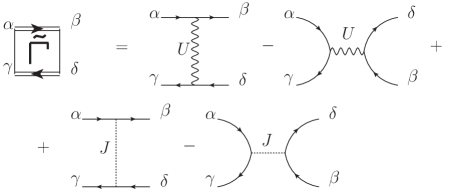
Figure 2: Structure of the particle-hole vertex, ${\tilde{\Gamma}\;}_{\alpha\gamma}^{\beta\delta}$. Here $\alpha$, $\beta$, $\gamma$ and $\delta$ denote composite indices as introduced in Eq. (21)

(a)

(b)

Figure 3: (a) Series of self-energy diagrams generated from $\Phi_{\rm FLEX}$. (b) Diagrammatic definition of the full particle-hole propagator, $\Pi$.

Differentiating the functional $\Phi$ of Fig. 1, one obtains the self-energy diagrams shown in Fig. 3.a. We then observe that all higher order diagrams contain the ladder series, shown in Fig. 3.b. Let us therefore introduce the composite label,

$$(l_{i},\sigma_{i},\kappa_{i})\to\alpha_{i}\;,$$ (21)

and define the particle-hole propagator, $\Pi^{(0)}$ as

$${\Pi^{(0)}}_{\alpha_{1}\beta_{1}}^{\alpha_{2}\beta_{2}}(t-t^{\prime})\equiv i^{2}G_{\alpha_{1}}^{\alpha_{2}}(t-t^{\prime})G_{\beta_{2}}^{\beta_{1}}(t^{\prime}-t)\;.$$ (22)

Then the full particle-hole propagator, $\Pi$, defined by the ladder series in Fig. 3.b. satisfies the following Dyson equation:

$$\Pi_{\alpha\beta}^{\alpha^{\prime}\beta^{\prime}}(t-t^{\prime})={\Pi^{(0)}}_{\alpha\beta}^{\alpha^{\prime}\beta^{\prime}}(t-t^{\prime})$$ (23)

$$-i\sum_{\scriptstyle\alpha_{1},\beta_{1}\atop\alpha_{2},\beta_{2}}\;\int\limits_{-\infty}^{\infty}{\rm d}\tilde{t}\;{\Pi^{(0)}}_{\alpha\beta}^{\alpha_{1}\beta_{1}}(t-\tilde{t})\tilde{\Gamma}_{\alpha_{1},\beta_{1}}^{\alpha_{2},\beta_{2}}\;{\Pi}_{\alpha_{2}\beta_{2}}^{\alpha^{\prime}\beta^{\prime}}(\tilde{t}-t^{\prime})\;.$$

The integral being just a convolution, this equation can be solved in Fourier space. Defining then

$${\Sigma_{\alpha}^{\beta}}_{\rm ladder}(t-t^{\prime})\equiv$$ (24)

$$\phantom{nn}-\sum_{\tilde{\alpha},\tilde{\beta}}\sum_{\scriptstyle\alpha_{1},\beta_{1}\atop\alpha_{2},\beta_{2}}\tilde{\Gamma}_{\alpha\tilde{\alpha}}^{{\alpha}_{1}{\beta}_{1}}{\Pi}_{\alpha_{1}{\beta}_{1}}^{\alpha_{2}\beta_{2}}(t-t^{\prime})\tilde{\Gamma}_{\alpha_{2}\beta_{2}}^{\beta\tilde{\beta}}G_{\tilde{\alpha}}^{\tilde{\beta}}(t-t^{\prime})\;,$$

we can sum up all $n\geq 3$ order self-energy diagrams. The self-energy $\Sigma_{\rm ladder}$ also contains the second order self-energy contribution, but with double weight. Therefore, the total self-energy can be written as

$${\Sigma}=\Sigma_{\rm ladder}+\Sigma^{(1)}-\Sigma^{(2)}\;,$$ (25)

with the first and second order diagrams, $\Sigma^{(1)}$ and $\Sigma^{(2)}$ defined as

$${\Sigma^{(1)}}_{\alpha}^{\beta}=i\;\delta_{\kappa_{\alpha}\kappa_{\beta}}s_{\kappa}\int\limits_{-\infty}^{\infty}\frac{d\omega_{1}}{2\pi}\sum_{\tilde{\alpha}\tilde{\beta}}{{\tilde{\Gamma}}}_{\alpha\beta}^{\tilde{\alpha}\tilde{\beta}}{G_{\tilde{\alpha}}^{\tilde{\beta}}}^{<}(\omega_{1})\;,$$

$${{\Sigma^{(2)}}_{\alpha}^{\beta}}(t-t^{\prime})\;$$

$$= -\frac{1}{2}\sum_{\tilde{\alpha},\tilde{\beta}}\sum_{\scriptstyle\alpha_{1},\beta_{1}\atop\alpha_{2},\beta_{2}}\tilde{\Gamma}_{\alpha\tilde{\alpha}}^{{\alpha}_{1}{\beta}_{1}}{\Pi^{(0)}}_{\alpha_{1}{\beta}_{1}}^{\alpha_{2}\beta_{2}}(t-t^{\prime})\tilde{\Gamma}_{\alpha_{2}\beta_{2}}^{\beta\tilde{\beta}}G_{\tilde{\alpha}}^{\tilde{\beta}}(t-t^{\prime})\;.$$

Solving the equations above turns out to be numerically rather demanding for two reasons: First, to get a good enough time resolution, we have to keep a large number of time (frequency) points in the calculations. Second, the propagator $\Pi$ has too many indices. In fact, even in our simple case, $\Pi$ has $8^{4}$ components. This number can be, however, substantially reduced if we exploit the SU(2) spin symmetry of the problem. Using simple group-theoretical arguments, we can show that the vertex $\tilde{\Gamma}$ assumes a simple form in spin space, and can be expressed in terms of a singlet and a triplet component,

$$\underline{\underline{\tilde{\Gamma}}}_{\sigma_{1}\sigma_{2}}^{\sigma_{3}\sigma_{4}}=\begin{bmatrix}\frac{1}{2}\left(\underline{\underline{\tilde{\Gamma}}}_{\;s}+\underline{\underline{\tilde{\Gamma}}}_{\;t}\right)&0&0&\frac{1}{2}\left(\underline{\underline{\tilde{\Gamma}}}_{\;s}-\underline{\underline{\tilde{\Gamma}}}_{\;t}\right)\\ 0&\underline{\underline{\tilde{\Gamma}}}_{\;t}&0&0\\ 0&0&\underline{\underline{\tilde{\Gamma}}}_{\;t}&0\\ \frac{1}{2}\left(\underline{\underline{\tilde{\Gamma}}}_{\;s}-\underline{\underline{\tilde{\Gamma}}}_{\;t}\right)&0&0&\frac{1}{2}\left(\underline{\underline{\tilde{\Gamma}}}_{s}+\underline{\underline{\tilde{\Gamma}}}_{t}\right)\;\end{bmatrix}\;,$$ (28)

with the four indices ordered as $\{\uparrow\uparrow,\uparrow\downarrow,\downarrow\uparrow,\downarrow\downarrow\}$, and the matrices $\underline{\underline{\tilde{\Gamma}}}_{s,t}$ defined as

$${\underline{\underline{\tilde{\Gamma}}}\;}_{t} = {\underline{\underline{\tilde{\Gamma}}}\;}_{\uparrow\uparrow}^{\uparrow\uparrow}-{\underline{\underline{\tilde{\Gamma}}}\;}_{\downarrow\downarrow}^{\uparrow\uparrow}\;,$$ (29)

$${\underline{\underline{\tilde{\Gamma}}}\;}_{s} = {\underline{\underline{\tilde{\Gamma}}}\;}_{\uparrow\uparrow}^{\uparrow\uparrow}+{\underline{\underline{\tilde{\Gamma}}}\;}_{\downarrow\downarrow}^{\uparrow\uparrow}\;.$$ (30)

Here each entry is a matrix in the remaining orbital ($l$) and Keldysh ($\kappa$) labels: $(\tilde{\Gamma}_{t,s})_{l_{1}\kappa_{1};l_{2}\kappa_{2}}^{l_{3}\kappa_{3};l_{4}\kappa_{4}}\to{\underline{\underline{\tilde{\Gamma}}}\;}_{t,s}$. By the same symmetry argument, we can show that the propagators $\Pi^{(0)}$ and $\Pi$ take on a similar form. Furthermore, it is easy to see that this structure is maintained under multiplication, where the lower indices of a tensor are contracted with the upper indices of another tensor. Therefore the singlet and the triplet components of $\Pi$ can be summed up independently:

$${\underline{\underline{\Pi}}\;}_{s,t}(\omega) = {\underline{\underline{\Pi}}\;}_{s,t}^{(0)}(\omega)\left[\underline{\underline{1}}+i\;{\underline{\underline{\tilde{\Gamma}}}\;}_{s,t}\;{\underline{\underline{\Pi}}\;}_{s,t}^{(0)}(\omega)\right]^{-1}\;,$$ (31)

with the unit matrix $\underline{\underline{1}}$ defined as $(\underline{\underline{1}})_{l_{1}\kappa_{1};l_{2}\kappa_{2}}^{l_{3}\kappa_{3};l_{4}\kappa_{4}}=\delta^{l_{3}}_{l_{1}}\delta^{l_{4}}_{l_{2}}\delta^{\kappa_{3}}_{\kappa_{1}}\delta^{\kappa_{4}}_{\kappa_{2}}\;$. We can then simply express the spin-independent part of $\Sigma_{\rm ladder}$ in terms of ${\underline{\underline{\Pi}}\;}_{s,t}$ as

$$({\Sigma_{\rm ladder}})_{p}^{q}(t)=-\sum_{\tilde{p},\tilde{q}}\frac{3}{2}\left(\underline{\underline{\tilde{\Gamma}}}_{\;t}\;\underline{\underline{\Pi}}_{\;t}(t)\;\underline{\underline{\tilde{\Gamma}}}_{\;t}\right)_{p\tilde{p}}^{q\tilde{q}}{G\;}_{\tilde{p}}^{\tilde{q}}(t)$$

$$\phantom{nnn}-\sum_{\tilde{p},\tilde{q}}\frac{1}{2}\left(\underline{\underline{\tilde{\Gamma}}}_{\;s}\;\underline{\underline{\Pi}}_{\;s}(t)\;\underline{\underline{\tilde{\Gamma}}}_{\;s}\right)_{p\tilde{p}}^{q\tilde{q}}\;{G\;}_{\tilde{p}}^{\tilde{q}}(t)\;,$$ (32)

with $p$ and $q$ denoting composite labels, only including the orbital and the Keldysh indices, $(l,\kappa)\to p,q$.

II.3 Details of the FLEX iteration

The previously defined equations provide a self-consistent set of equations, which we then solve iteratively. In 0’th order, we approximate the full Green’s function $\mathbf{G}$ by $\mathbf{g}$,

$${G^{[0]}}_{\alpha}^{\beta}(\omega) = g_{\alpha}^{\beta}(\omega)\;,$$ (33)

$${\Sigma^{[0]}}_{\alpha}^{\beta}(\omega) = 0\;.$$ (34)

We then start iteration $n\geq 1$, by first computing $\mathbf{G}^{[n-1]}(t)$ from the Green’s function $\mathbf{G}^{[n-1]}(\omega)$ of the previous iteration, by performing a Fast Fourier Transformation (FFT). Next, we construct $({{\underline{\underline{\Pi}}}}_{\;s,t}^{(0)})^{[n-1]}(t)$, obtain from that $({{\underline{\underline{\Pi}}}}_{\;s,t}^{(0)})^{[n-1]}(\omega)$, and then we solve the Dyson equation, Eq. (31) to get ${{\underline{\underline{\Pi}}}}_{\;s,t}^{[n-1]}(\omega)$. From that we obtain ${{\underline{\underline{\Pi}}}}_{\;s,t}^{[n-1]}(t)$ by FFT. We can then use ${\underline{\underline{\Pi}}}_{\;s,t}^{[n-1]}(t)$, $({{\underline{\underline{\Pi}}}}_{\;s,t}^{(0)})^{[n-1]}(t)$, and $\mathbf{G}^{[n-1]}(t)$ to compute $\mathbf{\Sigma}^{[n]}_{\rm ladder}$, $(\mathbf{\Sigma}^{(1)})^{[n]}$, and $(\mathbf{\Sigma}^{(2)})^{[n]}$, and finally the total self-energy, $\mathbf{\Sigma}^{[n]}(t)$, through equations Eq. (24), (II.2), (II.2) and (25). Finally, we obtain our next estimate, $\mathbf{G}^{[n]}(\omega)$, by first computing the Fourier transform, $\mathbf{\Sigma}^{[n]}(\omega)$, and inverting the Dyson equation, Eq. (14). This iteration procedure is repeated until convergence is reached.

In the numerical calculations we represented the Green’s functions using a finite uniform mesh of $N$ frequency points in the range $-\Omega/2<\omega<\Omega/2$. As mentioned above, the numerics was highly demanding; we had to use $2^{16}-2^{18}$ frequency points and $\Omega\approx 1000U$ to reach convergence. The memory demand of the calculation was also much higher than that of the iterative perturbation theory (IPT) procedure of Ref. prev, . With the symmetry-based representation of $\tilde{\Gamma}$ and $\Pi$ propagators, however, we managed to reduce the size of them substantially and were able to run the calculation on simple PC’s.

Although for small interaction parameters the convergence was rather stable, FLEX showed instabilities for high interaction parameters, similar to IPTprev . These instabilities could be partially cured by a gradual increase of the interaction parameters. With this trick, the range of applicability was found to be roughly the same as the one found with IPT.prev

III Results and Discussion

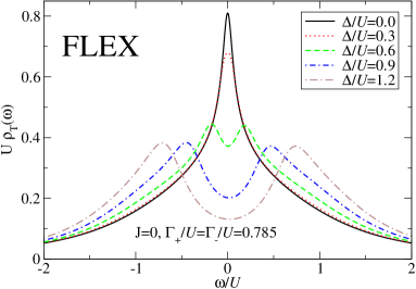
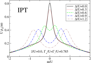
Figure 4: Total spectral function, $\rho_{T}(\omega)=(\rho_{+}(\omega)+\rho_{-}(\omega))/2$ for $J/U=0$ and $\Gamma_{\pm}/U=0.785$ for different values of level splitting, $\Delta/U$. On the top we show the FLEX results, while the bottom shows the IPT results for the same parameters.

Let us now turn to the presentation of the numerical results. For simplicity, excepting Subsection III.3, in this section we shall focus on a completely symmetrical dot with an even ($i=+$) and an odd ($i=-$) level. In this case, the tunneling matrix elements satisfy

$$t_{L\pm} = \pm\;t_{R\pm}\;,$$ (35)

and the tunnelings can be characterized simply by the widths of the levels,

$$\Gamma_{i}\equiv\sum_{\alpha=L,R}\Gamma^{\alpha}_{ii}\;,$$ (36)

both for lateral and for vertical dots. Similar to Ref. prev, , here we shall focus onto the vicinity of the electron-hole symmetrical point, $\tilde{\varepsilon}_{+}=\tilde{\varepsilon}_{-}=0$, and assume that the two levels are symmetrically positioned,

$$\tilde{\varepsilon}_{\pm}=\pm\Delta/2\;.$$ (37)

III.1 The case $\Gamma_{+}=\Gamma_{-}$

III.1.1 Equilibrium spectral functions

In this case, for $\Delta=J=0$, the three singlet and the triplet states of an isolated doubly occupied dot are completely degenerate, and an unusual Kondo state is formed.prev ; avishai Turning on $\Delta$, one separates the singlet state with both electrons on state $i=-$ from the rest of the states, and destroys the Kondo effect once $\Delta$ becomes larger than the Kondo temperature, $T_{K}^{*}$, defined as the halfwidth of the central peak for $\Delta=J=0$. This transition can be observed in the total equilibrium spectral functions,

$$\rho_{T}(\omega)=-\sum_{i=\pm}\frac{1}{2\pi}\mathrm{Im}\;G_{\;i,i}^{R}(\omega)\;,$$ (38)

where the retarded Green’s function is defined as,

$$G_{i,j}^{R}\equiv G^{i1}_{j1}-G^{i1}_{j2}={G}_{i,j}^{T}-{G}_{i,j}^{<}\;,$$ (39)

with ${G}_{i,j}^{T}\equiv{G}^{i1}_{j1}$ the time-ordered Green’s function.

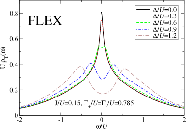
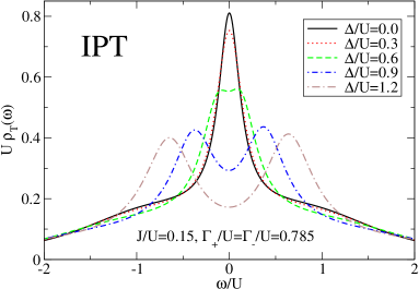
Figure 5: Total equilibrium spectral function, $\rho_{T}(\omega)$ for $J/U=0.15$ and $\Gamma_{\pm}/U=0.785$ for different values of level splitting, $\Delta/U$, as computed by FLEX (top) and by IPT (bottom).

In Fig. 4, we display $\rho_{T}(\omega)$ for $J=0$ for various splittings of the two levels, $\Delta$, as computed by FLEX and by the iterated perturbation theory (IPT) of Ref. prev, . The splitting of the Kondo resonance is remarkably similar in the two figures, however, there are important differences, too. First of all, FLEX gives a smaller Kondo temperature, and provides a more realistic shape for the Kondo resonance both in the absence and in the presence of splitting. However, while the Hubbard peaks at $\omega=\pm U$ are still visible within the simple perturbative calculation, FLEX is unable to capture them correctly.

Similar conclusions are reached for $J\neq 0$ with the exception that now the splitting of the Kondo resonance is shifted to higher values of $\Delta$ (see Fig. 5). However, in this case the central peak has a slightly different interpretation than for $J=0$, since for $J>0$ the isolated dot would be in a triplet state. As a result, the central Kondo resonance at $\Delta=0$ can be interpreted as a result of a triplet Kondo effect, where the spin $S=1$ of the dot is screened by the even and the odd conduction electron channels. In this triplet state the ground state degeneracy of the isolated dot is reduced, and quantum fluctuations are therefore somewhat suppressed. As a consequence, the Kondo temperature $T_{K}$ is also reduced, and the central peak becomes slightly narrower, but also more stable against $\Delta\neq 0$; in this $J>0$ case the splitting of the triplet Kondo resonance occurs roughly when $\Delta\sim 2J+T_{K}$.

III.1.2 Comparison with numerical renormalization group

Before entering the discussion of the non-equilibrium results, it is worth comparing FLEX with other methods such as iterative perturbation theory (IPT), or numerical renormalization group calculations (NRG),Wilson ; Bulla the latter procedure giving us a benchmark for the equilibrium calculations. Fig. 6 compares the results of these three methods for parameters $\Delta=0$, $\Gamma_{\pm}/U=0.785$, and $J/U=0.15$. For the NRG calculations we used the open access Budapest NRG code.BpNRG To reduce computational effort and achieve sufficient accuracy, we made use of the spin SU(2) symmetry of the Hamiltonian, as well as the $U(1)$ symmetries corresponding to the conservation of the total fermion numbers in channels $i=\pm$. The computations were performed with a discretization parameter, $\Lambda=2$, and 2400 kept multiplets. The calibration of the NRG parameters requires special care, since the NRG discretization and iteration procedure renormalizes somewhat the bare parameters of the Hamiltonian.Wilson ; Oliveira We calibrated the level widths $\Gamma_{\pm}$ from the height of the numerically calculated spectral functions. The results obtained this way were in good agreement with the analytical expressions of Ref. Oliveira, .

As shown in Fig. 6 the width of the Kondo resonance is perfectly captured by FLEX for the above parameters, while IPT slightly overestimates the size of the Kondo resonance. (As a comparison, in Fig. 6 we also plotted the shape of the resonance for $U=0$.) However, while FLEX seems to give a better estimate for the Kondo temperature than IPT, IPT seems to capture the high-energy features (Hubbard peaks) better – a well-known shortcoming of FLEX.JAWhite

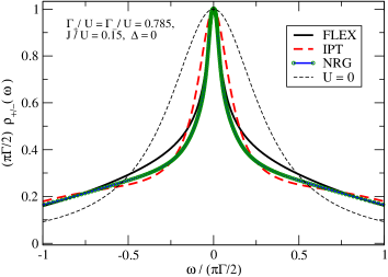
Figure 6: Comparison of the spectral functions for $\Delta=0$, $\Gamma_{\pm}/U=0.785$, and $J/U=0.15$, as computed by FLEX, IPT, and NRG. Clearly, FLEX seems to capture rather accurately the width of the central Kondo resonance.

III.2 The asymmetric case, $\Gamma_{+}\neq\Gamma_{-}$

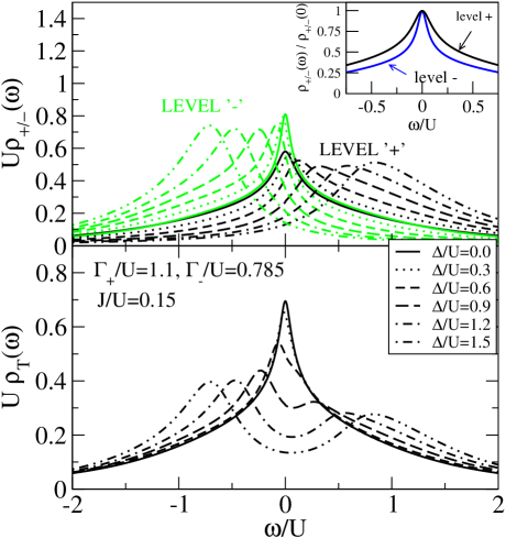
Figure 7: Level-resolved (top) and total (bottom) equilibrium spectral functions for $J/U=0.15$, $\Gamma_{+}/U=1.1$ and $\Gamma_{-}/U=0.785$ for different level splittings, $\Delta/U$, as computed by FLEX. The inset in the upper panel shows the normalized spectral functions $\rho_{\pm}(\omega)/\rho_{\pm}(0)$, demonstrating the presence of the two different Kondo scales.

Let us now turn to the more generic situation, $\Gamma_{+}\neq\Gamma_{-}$, and $J>0$. In this case, for $\Delta\approx 0$, the triplet spin on the dot is screened by a two-stage Kondo effect,Pust and the central resonances in the level-projected spectral functions, $\rho_{\pm}(\omega)$, become different due to the presence of two different Kondo scales, $T_{K}^{\pm}$, corresponding to the screening in the even and in the odd channels, respectively.

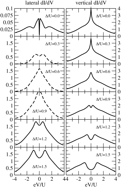
Figure 8: Differential conductance, $G(V)={\rm d}I/{\rm d}V$, in units of $e^{2}/h$ for lateral (l.h.s.) and vertical (r.h.s.) dots, with $J/U=0.15$, $\Gamma_{+}/U=0.785$, and $\Gamma_{-}/U=1.1$ for different level splittings, $\Delta/U$, as obtained by FLEX. On the triplet side ($\Delta=0$), the second Kondo scale emerges as a narrow dip/sharp resonance in $G(V)$ in the lateral/vertical arrangement. For large $\Delta$’s the singlet-triplet splitting gives rise to a wide central dip in $G(V)$. The curves reproduce very nicely all experimentally observed features, however, the cross-over regime is only qualitatively captured in the lateral case.

In Fig. 7 we show the level-projected as well as the full spectral functions, $\rho_{T}(\omega)$, as computed by FLEX for a dot with $J/U=0.15$, $\Gamma_{+}/U=1.1$ and $\Gamma_{-}/U=0.785$ for different level splittings, $\Delta/U$. Unlike for $\Gamma_{+}=\Gamma_{-}$, for $\Delta=0$ the projected spectral functions of the two levels are different, $\rho_{+}(\omega)\neq\rho_{-}(\omega)$. Nevertheless, they are all symmetrical as a consequence of a discrete particle-hole symmetry (see Ref. prev, ). However, this symmetry is violated for any $\Delta\neq 0$, where electron-hole symmetry is destroyed even for the total spectral function, $\rho_{T}(\omega)$. The difference in the Kondo temperatures is clearly visible in the normalized level-projected spectral functions, shown in the inset of Fig. 7.

Similar to the symmetrical case, the Kondo resonances are gradually split by a finite $\Delta$. The splitting of the resonances appears even more strikingly in the differential conductance, $G(V)={\rm d}I/{\rm d}V$, as computed from Eq. (II.2), and shown in Fig. 8. These differential conductance curves were obtained by computing $\mathbf{G}$ and $I(V)$ for each bias voltage $V$ separately, and then carrying out a numerical differentiation.

For a lateral dot at $\Delta=0$, i.e. in the two-stage Kondo effect regime, the ${\rm d}I/{\rm d}V$ curve shows very nicely the build-up of the first Kondo resonance,Wiel ; Granger and then the appearance of a dip at $V=0$ bias. This dip is a result of the destructive interference between the two Kondo effects, and it appears once the bias voltage becomes so small that it cannot destroy even the narrower Kondo resonance of the spectral function. As shown in Fig. 9, increasing $\Delta$, the linear conductance (i.e., the zero bias differential conductance) exhibits a maximum in the cross-over regime, in agreement with the experiments. However, the bias-dependence of the differential conductance in the cross-over regime (dashed lines in Fig. 8) of maximal conductance is not very reliable, and the $G(V)$ only shows the general trends observed experimentally, i.e., the disappearance of the central dip, and the appearance of a state with a single Kondo resonance and a perfect $G=2e^{2}/h$ linear conductance. For even larger $\Delta$’s, however, the ${\rm d}I/{\rm d}V$ curves show very nicely the linear splitting of the Kondo resonance.

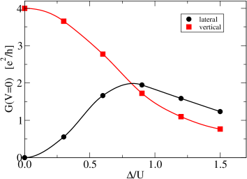
Figure 9: Linear conductance, for lateral and vertical dots, with $J/U=0.15$, $\Gamma_{+}/U=0.785$, and $\Gamma_{-}/U=1.1$ for different level splittings, $\Delta/U$, as obtained by FLEX.

In contrast to the lateral case, in a vertical geometry, the second Kondo effect manifests itself as an additional contribution to the conductance, and thus as a narrow peak at zero bias for $\Delta=0$. In this vertical case, the differential conductance curves reproduce the experimentally observed features even in the cross-over regime: the linear conductance is suppressed with increasing $\Delta$ (see Fig. 9), and the central resonance gets gradually broader, until it splits into two side-peaks, corresponding to the singlet-triplet excitation energy.

Finally, for a comparison, in Fig. 10 we show the ${\rm d}I/{\rm d}V$ curves at $\Delta=0$, as obtained by IPT, for the same parameters as the ones used to produce Fig. 8. The IPT curves are strikingly similar in structure to the ones obtained by FLEX. The most important difference is in the width of the central dip/resonance structure, which is somewhat narrower in the FLEX calculation, and is closer to the real value.

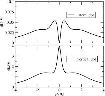
Figure 10: Differential conductance (in units of $e^{2}/h$) of a vertical and a lateral dot with $J/U=0.15$, $\Gamma_{+}/U=1.1$, $\Gamma_{-}/U=0.785$, and $\Delta=0$, as obtained by IPT. The curves compare quite well with the ones in Fig. 8.

III.3 The fully asymmetrical case

So far, we focused on the case of a completely symmetrical quantum dot, and correspondingly, we assumed that one of the states is even while the other state is odd. In general, however, quantum dots are not entirely symmetrical. Such asymmetry leads to the suppression of the maximal conductance, and for lateral quantum dots it may also lead to interference effects.Meden It is out of the scope of the present paper to study such interference effects in detail, however, to demonstrate how FLEX works in this more general case, let us present here some results.

In this general case, we can parametrize the tunneling to the leads using the angles $\phi_{\pm}\in[-\pi/2,\pi/2]$ as

$$(t_{\pm,L},t_{\pm,R})=t_{\pm}\;(\cos(\phi_{\pm}),\sin(\phi_{\pm}))\;.$$ (40)

For an even level, $\phi=\pi/4$, while for an odd level, $\phi=-\pi/4$.

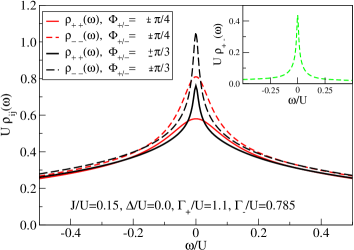
Figure 11: Equilibrium dimensionless spectral functions for $J/U=0.15$ $\Gamma_{+}/U=1.1$, $\Gamma_{-}/U=0.785$, $\Delta/U=0$ for a symmetrical dot with $\phi_{\pm}=\pm\pi/4$ and for an asymmetrical dot with $\phi_{\pm}=\pm\pi/3$, as computed by FLEX. The inset shows the off-diagonal component of the spectral function for $\phi_{\pm}=\pm\pi/3$.

In Fig. 11 we present the equilibrium spectral functions,

$$\rho_{ij}(\omega)\equiv\frac{i}{2\pi}(G_{ij}^{R}(\omega)-G_{ij}^{A}(\omega))\;,$$

for the same level width, $\Gamma_{+}/U=1.1$, and $\Gamma_{-}/U=0.785$ as before, but for a lateral dot with $\phi_{\pm}=\pm\pi/3$. In this case left-right symmetry is absent, and $\rho_{ij}$ has offdiagonal components, too. Interference between the states $\pm$ appears as a resonant structure in $\rho_{+-}$. However, in contrast to the components $\rho_{++}$ and $\rho_{--}$, within numerical accuracy $\rho_{+-}$ and $\rho_{-+}$ integrate to zero according to the corresponding spectral sum rule. For $\Delta=0$ the dot is still electron-hole symmetrical, and the heights of the spectral functions at $\omega=0$ are simply given by

$$\rho_{ij}(0)=\frac{2}{\pi}(\mathbf{\Gamma}^{-1})_{ij}\;,$$ (41)

with $\Gamma_{ij}=\sum_{\alpha=L,R}\Gamma^{\alpha}_{ij}$ the full relaxation rates (see Eq. (36)), as can be checked by an explicit calculation.

Fig. 12 shows and compares the differential conductance computed for asymmetric vertical and lateral dots in the triplet regime ($\Delta=0$). The curves are very similar to the ones obtained for symmetrical dots, excepting two important differences: (a) The conductance of a vertical dot does not reach the unitary conductance but goes only up to the value $2e^{2}/h\;(\sin^{2}(2\phi_{+})+\sin^{2}(2\phi_{-}))=3e^{2}/h$, and similarly, the overall conductance of a lateral dot is also suppressed. (b) The width of the narrower resonance is reduced for a lateral dot. This is due to the fact that the smaller eigenvalues of the $\mathbf{\Gamma}$ matrix are reduced by the interference as

$$\tilde{\Gamma}_{-} = \frac{\Gamma_{+}+\Gamma_{-}}{2}$$

$$- \sqrt{\frac{(\Gamma_{+}-\Gamma_{-})^{2}}{4}+\Gamma_{+}\Gamma_{-}\cos^{2}(\phi_{+}-\phi_{-})}\;,$$

and accordingly, the dip corresponding to the narrow Kondo resonance becomes also narrower. In contrast, the structure of the ${\rm d}I/{\rm d}V$ curve remains essentially unaltered for a vertical dot, where only the amplitude of the signal is reduced.

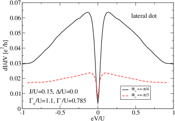
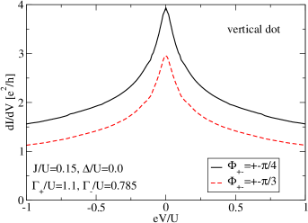
Figure 12: Top: Differential conductance, $G(V)={\rm d}I/{\rm d}V$, for lateral (top) and vertical (bottom) dots with $J/U=0.15$, $\Gamma_{+}/U=0.785$, $\Gamma_{-}/U=1.1$ and $\Delta/U=0$, as obtained by FLEX, for the symmetrical case, $\phi_{\pm}=\pm\pi/4$, and for the asymmetrical case, $\phi_{\pm}=\pm\pi/3$.

IV Conclusions

In the present paper, we developed a general non-equilibrium fluctuation exchange approximation (FLEX) formalism. We tested the performance of this approach on the singlet-triplet transition of a dot with two single-particle levels, driven by a competition between the Hund’s rule coupling and the Kondo screening. This transition exhibits several correlation-induced features, which are typically rather difficult to capture. On the triplet side of the transition a Kondo state develops with two different Kondo scales, while on the other side of the transition the triplet excitation appears as a pseudogap feature. Finally, in the cross-over region an exotic Kondo state appears, and for a lateral dot the linear conductance shows a broad resonance.

Remarkably, within its range of convergence, FLEX was able to capture all these features, excepting the Hubbard peaks, which are rather poorly represented by FLEX. Nevertheless, the low energy features and the ${\rm d}I/{\rm d}V$ curves show behaviors remarkably close to the experimentally observed ones. In our earlier studies, we applied simple (iterative) perturbation theory (IPT) to describe the singlet-triplet transition. FLEX has some clear advantages, but also disadvantages with respect to IPT. On the one hand, it produces apparently more realistic curves in the small bias region than IPT, and – as our comparison with NRG calculations confirms – it captures the Kondo temperature as well as the Kondo effect-related structures better there. In addition, it is a generically conserving approximation, and it scales rather well with the number of orbitals. All these properties make FLEX a viable route to incorporate strong correlation effects in molecular electronics calculations. On the other hand, FLEX is computationally much more demanding. In fact, in this work we had to exploit symmetries to reduce the computational effort. This is, of course, not a major obstacle if one has access to supercomputers or efficient computer clusters, and we believe that the numerical efficiency can most likely be further improved.

Finally, let us comment on the version of FLEX we used here. In the present paper, we used a generating $\Phi$-functional, which only incorporates electron-hole bubble series. FLEX can, however, be extended to include fluctuations in the Cooper channel, too. This may be important in cases, where attractive interactions appear in some scattering channels. In particular, such an extension of FLEX may be necessary to describe transport through superconducting grains. The generalization is relatively straightforward, however, it is certainly beyond the scope of the present work, which solely focused on the demonstration of FLEX as an efficient non-equilibrium impurity solver.

V Acknowledgment

This research has been supported by the Hungarian Scientific Research Funds Nos. K73361, CNK80991, NN76727, TÁMOP-4.2.1/B-09/1/KMR-2010-0002, and the EU-NKTH GEOMDISS project. G.Z. also acknowledges support from the Alexander von Humboldt Foundation. We would also like to thank Pascu Moca for kindly helping us to use special features of the yet unpublished new version of the Budapest NRG code.

Appendix A The hybridized Green’s function, $\mathbf{g}$

For completeness, let us give here the elements of $\mathbf{g}^{-1}(\omega)$. Restricting ourselves to the spin symmetrical case, ${g^{-1}}_{i\sigma\kappa}^{j\sigma^{\prime}\kappa^{\prime}}=\delta_{\sigma}^{\sigma^{\prime}}\;{g^{-1}}_{i\kappa}^{j\kappa^{\prime}}$. The elements of ${g^{-1}}_{i\kappa}^{j\kappa^{\prime}}$ differ for lateral and vertical dots. For lateral dots, they are given by

$${(g^{-1}_{\rm\;lat})}_{i\kappa}^{j\kappa^{\prime}} = {\delta\;}_{i}^{j}s(\kappa)\left(\omega-\tilde{\varepsilon}_{i}\right)\delta_{\kappa}^{\kappa^{\prime}}$$ (42)

$$- \sum_{\alpha\in L,R}N_{\alpha}\;t^{*}_{\alpha i}t_{\alpha j}\;\Delta_{\alpha}^{\kappa\kappa^{\prime}}(\omega)\;,$$

with $s(\kappa)$ the Keldysh sign defined in the main text, and hybridization parameters $\Delta_{\alpha}^{\kappa\kappa^{\prime}}(\omega)$ defined as

$$\Delta_{\alpha}^{11}(\omega) = \pi i(2f_{\alpha}(\omega)-1)\;,$$ (43)

$$\Delta_{\alpha}^{12}(\omega) = -2\pi if_{\alpha}(\omega)\;,$$ (44)

$$\Delta_{\alpha}^{21}(\omega) = -2\pi i(f_{\alpha}(\omega)-1)\;,$$ (45)

$$\Delta_{\alpha}^{22}(\omega) = \pi i(2f_{\alpha}(\omega)-1)\;,$$ (46)

with $f_{\alpha}(\omega)=f(\omega-eV_{\alpha})$ the shifted Fermi function. For vertical dots, on the other hand, ${g^{-1}}_{i\kappa}^{j\kappa^{\prime}}$ is diagonal in $i$ and $j$,

$${(g^{-1}_{\rm\;vert})}_{i\kappa}^{j\kappa^{\prime}} = {\delta\;}_{i}^{j}s(\kappa)\left(\omega-\tilde{\varepsilon}_{i}\right)\delta_{\kappa}^{\kappa^{\prime}}$$ (47)

$$- {\delta\;}_{i}^{j}\sum_{\alpha\in L,R}N_{\alpha\;i}\;|t_{\alpha i}|^{2}\;\Delta_{\alpha}^{\kappa\kappa^{\prime}}(\omega)\;.$$

References

- (1) H. B. Heersche, PhD Thesis, Delft Technical University, Nederland (2006).
- (2) G. D. Scott and D. Natelson, arXiv:cond-mat/1003.1938 (2010).
- (3) N. Roch, S. Florens, V. Bouchiat, W. Wernsdorfer and F. Balestro, Nature 453, 633 (2008).
- (4) H. B. Heersche, Z. de Groot, J. A. Folk, H. S. J. van der Zant, C. Romeike, M. R. Wegewijs, L. Zobbi, D. Barreca, E. Tondello, and A. Cornia, Phys. Rev. Lett. 96, 206801 (2006).
- (5) J. Park, A. N. Pasupathy, J. I. Goldsmith, C. Chang, Y. Yaish, J. R. Petta, M. Rinkoski, J. P. Sethna, H. D. Abruna, P. L. McEuen and D. C. Ralph, Nature 417, 722 (2002).
- (6) W. Liang, M. P. Shores†, M. Bockrath, J. R. Long and H. Park, Nature 417, 725 (2002).
- (7) J. Eckel, F. Heidrich-Meisner, S. G. Jakobs, M. Thorwart, M. Pletyukhov and R. Egger, New. J. Phys. 12, 043042 (2010).
- (8) K.C. Nowack, F.H.L Koppens, Y.V. Nazarov, et al., Science 318, 5855 (2007).
- (9) F.H.L Koppens, J.A. Folk, J.M. Elzerman, et al., Science 309, 1346 (2005).
- (10) R. Hanson, L.H.V. van Beveren, I.T. Vink, et al., Phys. Rev. Lett. 94, 196802 (2005).
- (11) J. E. Han, Phys. Rev. B 81, 245107 (2010).
- (12) P. Mehta and N. Andrei, Phys. Rev. Lett 96, 216802 (2006), see also the correction in: P. Mehta, S. P. Chao and N. Andrei, arXiv:cond-mat/0703426 (2007).
- (13) E. Boulat, H. Saleur and P. Schmitteckert, Phys. Rev. Lett. 101, 140601 (2008).
- (14) Paaske J, Rosch A, Wolfle P, et al., Nature Physics 2, 460 (2006).
- (15) S. G. Jakobs, M. Pletyukhov and H. Schoeller, Phys. Rev. B 81, 195109 (2010).
- (16) M. Moeckel, S. Kehrein, Ann. Phys. 324, 2146 (2009).
- (17) S. Andergassen, V. Meden, H. Schoeller, J. Splettstoesser and M. R. Wegewijs, Nanotechnology 21, 272001 (2010).
- (18) F. B. Anders and A. Schiller, Phys. Rev. Lett. 95, 196801 (2005).
- (19) U. Schollwöck, Rev. Mod. Phys. 77, 259 (2005).
- (20) J. K. Freericks, V. M. Turkowski and V. Zlatic, Phys. Rev. Lett. 97, 266408 (2006).
- (21) J. Eckel, F. Heidrich-Meisner, S. G. Jakobs, M. Thorwart, M. Pletyukhov and R. Egger, New. J. Phys. 12, 043042 (2010).
- (22) K. Yosida and K. Yamada, Prog. Theor. Phys. 46, 244 (1970);
- (23) K. Yamada, Prog. Theor. Phys. 53, 970, (1975); K. Yosida and K. Yamada, Prog. Theor. Phys. 53, 1286 (1975); K. Yamada, Prog. Theor. Phys. 54, 316 (1975).
- (24) B. Horvatic and V. Zlatic, Phys. Status Solidi B 99, 251 (1980).
- (25) B. Horvatic, D. Sokcevic and V. Zlatic, Phys. Rev. B 36, 675 (1987).
- (26) A. C. Hewson, The Kondo Problem to Heavy Fermions (Cambridge University Press, Cambridge, 1993).
- (27) P. Nozieres and A. Blandin, J. Physique 39, 1117 (1978).
- (28) T. A. Costi, L. Bergqvist, A. Weichselbaum, et al., Phys. Rev. Lett. 102, 056802 (2009).
- (29) M. Pustilnik and L. I. Glazman, Phys. Rev. Lett. 85, 2993 (2000).
- (30) M. Pustilnik and L. I. Glazman, Phys. Rev. Lett. 87, 216601 (2001).
- (31) Matthias Vojta, Ralf Bulla, and Walter Hofstetter, Phys. Rev. B 65, 140405 (2002).
- (32) W. Hofstetter and G. Zaránd, Phys. Rev. B 69, 235301 (2004).
- (33) S. Sasaki, S. De Franceschi, J. M. Elzerman, W. G. van der Wiel, M. Eto, S. Tarucha and L. P. Kouwenhoven, Nature 405, 764 (2000).
- (34) W. G. van der Wiel, S. De Franceschi, J. M. Elzerman, S. Tarucha, L. P. Kouwenhoven, J. Motohisa, F. Nakajima, and T. Fukui, Phys. Rev. Lett. 88, 126803. (2002).
- (35) G. Granger, M. A. Kastner, Iuliana Radu, M. P. Hanson and A. C. Gossard, Phys. Rev. B 72, 165309 (2005).
- (36) J. Nygard, D. H. Cobden and P. E. Lindelof, Nature 408, 342 (2000).
- (37) P. R. Bas and A. A. Aligia, J. Phys.: Condens. Matter 22, 025602 (2010).
- (38) B. Horváth, B. Lazarovits and G. Zaránd, Phys. Rev. B 82, 165129 (2010).
- (39) G. Baym and L. P. Kadanoff, Phys. Rev. 124, 287 (1961).
- (40) G. Baym, Phys. Rev. 127, 1391 (1962).
- (41) N. E. Bickers, D. J. Scalapino and S. R. White, Phys. Rev. Lett. 62, 961 (1989); N. E. Bickers and D. J. Scalapino, Ann. Phys. (N.Y.) 193, 206 (1989).
- (42) N. E. Bickers and S. R. White, Phys. Rev. B 43, 8044 (1991).
- (43) J.A. White, Phys. Rev. B 45, 1100 (1992).
- (44) L. V. Pourovskii, M. I. Katsnelson and A. I. Lichtenstein, Phys. Rev. B 72, 115106 (2005).
- (45) A. I. Lichtenstein and M. I. Katsnelson, Phys. Rev. B 57, 6884 (1998).
- (46) M. I. Katsnelson and A. I. Lichtenstein, J. Phys.: Condens. Matter 11, 1037 (1999).
- (47) T. Kuzmenko, K. Kikoin and Y. Avishai, Phys. Rev. B 69, 195109 (2004).
- (48) K. G. Wilson, Rev. Mod. Phys. 47, 773 (1975).
- (49) R. Bulla, T. A. Costi, and T. Pruschke, Rev. Mod. Phys. 80, 395 (2008).
- (50) The open access code can be downloaded from: http://neumann.phy.bme.hu/ dmnrg/. For a description of the code, see: O. Legeza, C. P. Moca, A. I. Tóth, I. Weymann, G. Zaránd, arXiv:0809.3143 (2008); See also A. I. Tóth, C. P. Moca, O. Legeza, and G. Zaránd, Phys. Rev. B 78, 245109 (2008).
- (51) W.C. Oliveira and L.N. Oliveira, Phys. Rev. B 49, 11986 (1994).
- (52) V. Meden and F. Marquardt, Phys. Rev. Lett. 96, 146801 (2006). Levels on the double dot studied here act in a similar way as levels in our case.