Dynamic Defragmentation of Reconfigurable Devices

Abstract

We propose a new method for defragmenting the module layout of a reconfigurable device, enabled by a novel approach for dealing with communication needs between relocated modules and with inhomogeneities found in commonly used FPGAs. Our method is based on dynamic relocation of module positions during runtime, with only very little reconfiguration overhead; the objective is to maximize the length of contiguous free space that is available for new modules. We describe a number of algorithmic aspects of good defragmentation, and present an optimization method based on tabu search. Experimental results indicate that we can improve the quality of module layout by roughly 50% over static layout. Among other benefits, this improvement avoids unnecessary rejections of modules.

1 Introduction

1.1 Reconfiguration and Communication

FPGAs combine the performance of an ASIC implementation with the flexibility of software realizations. Partial runtime reconfiguration is an applicable technique to overcome significant area overhead, monetary cost, higher power consumption, or speed penalties as compared to ASICs (see e.g. [21]). By loading just the required modules to an FPGA at runtime, it is possible to build smaller systems and less power-hungry devices. For instance, an embedded system may start up with some boot-loader and test modules. These modules may be exchanged by a crypto-accelerator to speed up the authentication process of the user. Later, different modules will be loaded to the FPGA by partial runtime reconfiguration with respect to the user demand or the state of the system. Note that many systems provide mutually exclusive functionality (e.g., the record or the play mode of a multimedia device) that is suitable to share some FPGA resources at runtime. Furthermore, modules need to communicate with other modules to accomplish their tasks. Therefore, a suitable communication infrastructure must be applied and the implied costs in terms of time and area resources must be respected. This challenge and possible solutions are discussed in Section 2.

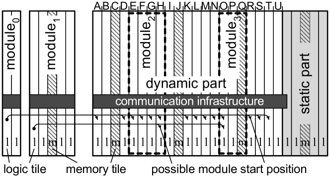
Figure 1: Dynamically reconfigurable, tile-oriented system. The system shares some logic tiles $l$ and memory tiles $m$ among a set of modules within the dynamic part of the system. Some modules require a memory tile at a fixed offset with respect to the start position within the modules (e.g., the third tile of module${}_{\textsf{1}}$ is a memory tile).

When using such systems, an efficient resource management becomes necessary. One problem that has to be solved at runtime is the fragmentation of the tiles due to the time-dependent execution of some modules on the same resource area. It is assumed that for dynamically partially reconfigurable systems, modules are to be vertically aligned column by column, as shown in Fig. 1. Accordingly, a module requiring multiple tiles to implement its logic will demand a consecutive adjacent set of tiles without any gaps. This problem is discussed in this paper.

1.2 Dynamic Storage Allocation on Reconfigurable Devices

The ever-increasing capabilities of modern reconfigurable devices give rise to a large number of new challenges; solving one of them in turn gives rise to new possibilities and challenges. As described above, there are new solutions for dealing with the communication of relocated devices; this opens up new possibilities for dynamic relocation of modules. The resulting challenge is the dynamic allocation of module requests to a reconfigurable device: given an array-shaped reconfigurable device and a sequence of module requests of varying resource requirements (e.g., logic tiles or memory blocks), assign each module to a contiguous set of slots on the device; see Fig. 2(a).

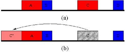
Figure 2: Dynamic storage allocation: (a) Each module occupies a contiguous block of array positions. (b) Moving a module to a new position in order to increase maximum free interval size.

At first glance, this problem has a striking resemblance to one of the classical problems of computing: Dynamic storage allocation considers a memory array and a sequence of storage requests of varying size, looking for an assignment of each request to a contiguous block of memory cells, such that the length of each block corresponds to the size of the request. Once this allocation has been performed, it is static in space: after a block has been occupied, it will remain fixed until the corresponding data is no longer needed and the block is released. As a consequence, a sequence of allocations and releases can result in fragmentation of the memory array, making it hard or even impossible to store new data.

Over the years, a large variety of methods and results for allocating storage have been proposed. The classical sequential fit algorithms, First Fit, Best Fit, Next Fit and Worst Fit can be found in Knuth [15] and Wilson et al. [24].

Buddy systems partition the storage into a number of standard block sizes and allocate a block in a free interval of the smallest standard size sufficient to contain the block. Differing only in the choice of the standard size, various buddy systems have been proposed [5, 12, 13, 14, 23, 15]. Newer approaches that use cache-oblivious structures for allocating space in memory hierarchies include the works by Bender et al. [3, 4].

There are notable differences between the dynamic allocation of modules to a reconfigurable device and dynamic storage allocation. First of all, all modules on a reconfigurable device may execute in parallel, while on a standalone processor, large blocks in memory are not used simultaneously. Reconfigurable devices do not provide techniques such as paging and virtual memory mapping that allow arranging memory blocks next to each other in a virtual way, while they are physically stored at non-adjacent positions. The reconfiguration of a module on a reconfigurable device implies delays, and an inter-module communication infrastructure is required, because the functionality of a reconfigurable device may depend on other modules and external periphery.

Modules on a reconfigurable device can be relocated to a different location on the reconfigurable device, this can even be done at runtime. However, today’s synthesis tools still lack support for placing a module implementation at different positions: these tools often allow placing a module at only one specific position; thus, we cannot use the same implementation binary for different positions on the reconfigurable device. Different techniques have been conceived to tackle this problem. One solution is to equip the reconfigurable device with a special reconfiguration-management unit that handles the modification of the module implementations at runtime such that they can be placed at the desired position. Moreover, in order to relocate a running module, the module must be paused, the state must be temporarily saved, the module must be reconfigured at the new position, the state must be restored, and the module must get a signal to continue its work. Different techniques have been developed for this task, one of them is presented by Koch et al. [18]. In the future, reconfigurable devices may have additional support for task preemption.

In contrast to memory and storage devices, reconfigurable devices often contain heterogeneities such as dedicated memories, DSPs, or CPUs. These units enable or increase performance in important application fields. But heterogeneities increase the complexity of defragmentation considerably: a module implementation possibly depends on a specific pattern of heterogeneous resources at the placement location in order to complete its task. The number of feasible positions of a module on a FPGA can be increased by creating different implementations of the same module (i.e., with different positions for the heterogeneities), but this approach also requires additional storage space for module implementations. Having different implementations of a module also increases the number of possibilities when defragmenting the module placements. Thus, the complexity of the defragmentation problem increases.

There is a huge amount of related work also from within the FPGA community: Becker et al. [1] present a method for enhancing the relocatability of partial reconfigurability of partial bitstreams for FPGA runtime configuration, with a special focus on heterogeneities. They study the underlying prerequisites and technical conditions for dynamic relocation. In the process, a method that circumvents the problem of having to find fully identical regions for the modules is solved by the creation of compatible subsets of resources, enabling a flexible placement of relocatable modules. Gericota et al. [10] present a relocation procedure for Configurable Logic Blocks (CLBs) that is able to carry out online rearrangements, defragmenting the available FPGA resources without disturbing functions currently running. Another relevant approach was given by Compton et al. [7], who present a new reconfigurable architecture design extension based on the ideas of relocation and defragmentation. It is shown that with little run-time effort on the part of the CPU and little additional area-increase over a basic partially reconfigurable FPGA, the reconfiguration overhead can be reduced tremendously. Koch et al. [16] introduce efficient hardware extensions to typical FPGA architectures in order to allow hardware task preemption. Furthermore, the technical aspects of applying hardware task preemption to avoid defragmentation are discussed. These papers do not consider the algorithmic implications and how the relocation capabilities can be exploited to optimize module layout in a fast, practical fashion, which is what we consider in this paper. Koester et al. [20] also address the problem of defragmentation. Different defragmentation algorithms that minimize different types of costs are analyzed. With the help of a simulation model and a benchmark, simulation results and algorithm comparisons are presented. However, the problem description differs in some major points; for example, no heterogeneities in the reconfigurable area are considered.

The general concept of defragmentation is well known, and has been applied to many fields, e.g., it is typically employed for memory management. Our approach is significantly different from defragmentation techniques which have been conceived so far: these require a freeze of the system, followed by a computation of the new layout and a complete reconfiguration of all modules at once. Instead, we just copy one module at a time, and simply switch the execution to the new module as soon as the move is complete. This leads to a seamless, dynamic defragmentation of the module layout, resulting in much better utilization of the available space for modules.

The rest of this paper is organized as follows. In the following Section 2 we give a description of the underlying model and assumptions of the reconfigurable device and application, giving rise to the problem description in Section 3. As it turns out, solving the corresponding optimization problem is NP-hard, as shown in Section 4. However, for moderate module density, it is still possible to compute optimal results, as shown in Section 5. In Section 6, we show that there are instances for which $\Omega(n^{2})$ moves are necessary. This leads to a heuristic optimization method for higher densities, based on tabu search and described in Section 7. Detailed experimental results are presented and discussed in Section 8 showing an increase in the maximal free space in average by $25\%$ when applying our defragmentation techniques for FPGAs with heterogeneities. On some inputs an increase up to $200\%$ is observed. Concluding thoughts are presented in Section 9.

2 Problem Scenario and Technical Challenges

Each partial reconfiguration of a module on a reconfigurable device incurs a certain amount of reconfiguration overhead. The ratio between the reconfiguration time and the actual running time of the corresponding modules is highly application specific. We assume in our scenario that the reconfiguration time is sufficiently small compared to the execution times of modules used. Of course, there are applications in which the reconfiguration overheads must be taken into account, because many different modules are loaded on the reconfigurable device and their execution times are not much higher than their reconfiguration times. However, the possibility of reconfiguring only a part of the reconfigurable device as well as techniques such as prefetching, latency hiding, and bitstream compression can significantly reduce the reconfiguration overheads. Furthermore, even today, for many applications a module’s reconfiguration time is much less than its execution time even today. So far, it is not known whether reconfiguration overheads will still play an important role for the performance of many applications in the future or not. In this paper, we assume that there will be also many applications in the future for which the reconfiguration overheads are no big issue.

In order to take more benefit from runtime reconfiguration, systems should be able to provide the reconfigurable resources in a very flexible way to the modules. Therefore, a communication infrastructure is required, such that modules can communicate with each other, and to peripheral input/output devices. Most related work for reconfigurable communication systems is still based on the assumption that the locations allowed for modules in a partially reconfigurable system are all fixed in size (e.g., Lysaght et al. [22]). Consequently, such approaches do not allow for exchanging a large module with multiple smaller ones. This originates from a lack of adequate communication techniques suitable to connect multiple partially reconfigurable modules within the same resource area to the rest of the system. However, there are notable exceptions: Koch et al. [17, 19] present a system with a reconfigurable area partitioned into 60 tiles, each capable of connecting a tiny 8-bit module to the system using the so-called ReCoBus. This allows it to implement larger interfaces or modules by combining multiple adjacent tiles; e.g., 4 tiles are required for building a 32-bit interface. In addition, the ReCoBus can link I/O pins to the partially reconfigurable modules. Furthermore, this approach of a reconfigurable bus demonstrates that high placement flexibility, low resource overhead, and high throughput can be achieved at the same time.

In some partially reconfigurable computing systems, module communication in a neighbor-to-neighbor-based manner is preferred to using a reconfigurable bus system: for example, FPGAs are also used in streaming applications, such as video processing and packet processing, where each module communicates concurrently with the next module in the pipeline such that the communication costs are kept low. If these systems will also benefit from defragmentation techniques highly depends on the communication constraints of the modules and on the individual reconfigurable computing system. In general, one option is to change the communication infrastructure of the modules to a more flexible system, such as a reconfigurable bus system. This may lead to increased communication costs, but at the same time, defragmentation techniques can place modules more freely, and thus yield better results. If the increase in communication costs is clearly amortized by the improvements due to better defragmentation results, then the reconfigurable system will benefit from this option. In a setting in which some modules in a reconfigurable computing system must be placed closely to each other (e.g., they may strongly rely on a fast neighbor-to-neighbor communication for performance reasons), these modules can be grouped together such that they are considered by the defragmentation strategy as a single module. Therefore, either all these modules are moved to another position for defragmentation, or no module is touched. Thus, defragmentation techniques for reconfigurable devices are flexible enough to accommodate all important technical aspects concerning module communication on FPGAs.

So far, there already exists an enormous and ever-growing number of different reconfigurable devices. Most of their reconfigurable area consists of heterogeneities, special-purpose units such as DSPs, CPUs, or RAMs, which offer a considerable performance improvement for target applications. See, for example, Fig. 1: this FPGA has two different column types, logic tiles ($l$) and memory tiles ($m$). The important challenge with heterogeneities are placement limitations: modules applying special-purpose units may not be freely relocated, but can be placed only at positions offering the same geometry of special purpose units; the placement of a module within the reconfigurable resource area on the FPGA must fit exactly to the particular module. Thus, the number of free tiles is not sufficient to determine whether a module can be placed. For instance, module${}_{\textsf{1}}$ in Fig. 1 has the resource requirement $l\,\,l\,m\,l\,\,l$ and can be placed only at the positions A, H, and O, which are currently occupied by module${}_{\textsf{2}}$ and module${}_{\textsf{3}}$. In the example, the system has 12 free logic tiles and 2 free memory tiles, but we are currently not able to place module${}_{\textsf{1}}$ on the FPGA, which requires just 4 logic tiles and 1 memory tile. Note that our approach does not depend on a specific type of heterogeneity, it can also be applied to future reconfigurable devices with new kinds of heterogeneities.

Our approach is targeted at currently available FPGAs and future reconfigurable devices. In our problem formulation, we assume a device that is capable of column-wise partial reconfiguration, i.e., only whole columns of the reconfigurable area are exchanged. Modern reconfigurable devices offer also the flexibility to reconfigure single cells in the reconfigurable area, but this kind of higher flexibility is not assumed in our problem formulation, because the column-wise reconfiguration is considered as an important case for these studies. Therefore, one reason may be that the applied device cannot provide that kind of higher flexibility, e.g., in order to save unnecessary costs. Many applications for reconfigurable devices work in a pipeline-based manner and employ modules that span over the whole column. They use only modules with the same heights, because allowing a greater level of flexibility concerning the placement would also imply higher resource overheads, e.g., in terms of communication resources. Furthermore, as long as the heights of all modules are equal, our approach can also be applied to cell-based reconfigurable devices using new abstraction layer: we introduce a new type of heterogeneity (the “’separating heterogeneity”) that is not used by any module. Then we simply connect the horizontal lines of cells of the device to form a single row, separated by this new heterogeneity; see Fig. 3. Thus, any placement of a module on the abstract device can be mapped to a placement on the original device.

\begin{picture}(11124.0,2724.0)(889.0,-4573.0)\end{picture}

Figure 3: Defragmenting a two-dimensional device. Left: A two-dimensional device. Right: The corresponding one-dimensional device with separating heterogeneities.

Our studies of the important case of column-based reconfiguration can also be applied to scenarios in which a cell-based reconfiguration and modules with differing heights are needed: the local search techniques applied in our approaches can also be used for finding another suitable place for a module in the two-dimensional space. The decision which steps to choose can also be extended from one to two dimensions. Thus, the proposed approach is not strictly limited to the important case of column-wise reconfiguration.

When modules are relocated for defragmentation, we have to distinguish between moving only the module configuration and the configuration together with the internal state. In the first case, we just make a copy of the reconfiguration data to the new position and start the next computation on the module at the new position (e.g., a discrete cosine transformation on the next frame in a video system). In the second case, both modules have to be interrupted and the state (represented by all internal flip-flop and memory values) will be copied to the target module. It may not be enough to copy the configuration data to a new position, because the configuration bit files often imply a certain position. Therefore, it is either necessary to alter dynamically the bit files, or to generate statically bit files for all possible positions. Relocation of modules and related problems were already addressed in other works. Furthermore, the communication between modules must be stalled during the relocation of the respective modules. Thus, the communication infrastructure should be flexible enough to meet these requirements. As compared to the reconfiguration process, copying the state can be performed with short interruption when using hardware checkpointing (for more details see Koch et al. [18]).

If we allow overlapping regions for the defragmentation, e.g., the source and the target module may overlap, then the interruption time can be dominated by the relocation process: an overlap prevents the possibility to copy the routing information and logic settings to the destination, while the original module is still running. In this case, the module must be stopped, the reconfiguration data and the state of the module must be copied to some (external) memory, and be restored at the destination. This procedure takes longer if the regions overlap. As a consequence, we will prevent our defragmentation algorithms from using overlapping regions to place modules. Thus, switching from the original module to the new one can be optimized in such a way, that no input data is lost, and the downtime of the module is minimized. Thus, a copy of module—without the state—can be reconfigured at the destination while the module is still running. Therefore, switching between the two modules is very fast for modules that have only few state data to be copied. Furthermore, our proposed defragmentation strategies move at most one module at a time to another position on the reconfigurable area. Thus, only a single module is affected at a moment by the defragmentation process, while the remaining set of modules remains untouched.

3 Problem Formulation

In this paper, we consider a reconfigurable device that allows allocating modules in a contiguous manner on an array $L$ of length $\ell$; modules will be denoted by $M_{1},\ldots,M_{n}$. A module $M_{i}$ placed in the array occupies a contiguous interval on the reconfigurable device, denoted by $L_{M_{i}}$. Modules are always placed such that $L_{M_{i}}\cap L_{M_{j}}=\emptyset$ for $i\neq j$; that is, two different modules do not overlap.

Modules placed in the array divide $L$ into sections that are occupied by a module and sections that are not occupied; the latter are called free intervals, denoted by $F_{1},\ldots,F_{k}$. Partially reconfigurable devices allow us to relocate a module $M_{i}$ of size $m_{i}$ from interval $L_{M_{i}}$ to a new position $L^{\prime}_{M_{i}}$ within a free interval $F_{j}$ of size $f_{j}$, provided that the following two conditions are fulfilled:

1. No occupied section is chosen (i.e., $L^{\prime}_{M_{i}}\cap\bigcup_{k=1}^{n}L_{M_{k}}=\emptyset$).

2. The size of the free interval is at least as big as the size of the module: (i.e., $f_{j}\geq m_{i}$).

The Maximum Defragmentation Problem (MDP) asks for a sequence of relocation moves that maximizes the size of the largest free interval on the reconfigurable device. We distinguish between the homogeneous MDP, in which every cell in the array is equivalent, and the heterogeneous MDP, which accounts for heterogeneities in the given FPGA. Clearly, the heterogeneous MDP is more difficult. Thus, we focus on the homogeneous MDP for our complexity results, as their harndess implies hardness of the more complicated, restricted versions.

Figure 4: Reducing 3-Partition to the MDP.

The larger free interval after the defragmentation can allow to place and execute a module that could not be placed before. Moreover, defragmentation helps to place modules at an earlier time. Altogether, the makespan is reduced, i.e., the total time that is needed to satisfy a sequence of requests (i.e., a sequence of modules $M_{1},\ldots,M_{n}$), considering that every module $M_{i}$ needs a certain time, the duration $T_{i}$, to run on the FPGA before it can be removed.

4 Problem Complexity

In this section, we state two complexity results for defragmenting modules on a reconfigurable device: one for deciding whether one contiguous free block can be formed, and one for the maximization version of the (homogeneous) defragmentation problem. We show that the decision version is strongly NP-complete and that no approximation algorithm with a useful approximation factor exists for the maximization version, unless P=NP.

We use a proof technique know as proof by reduction. That is, we take a problem that is known to be hard and show how to transform an instance of the known problem to an instance of our problem. Thus, if we had an efficient method for solving our problem, it could also be used for solving the other, hard problem. The problem 3-Partition is the main ingredient of the reduction. It belongs to the class of strongly NP-complete and can be stated as follows [9]:

Given:

A finite set of $3\cdot k$ elements $C_{1},\ldots,C_{3k}$ with sizes $c_{1},\ldots,c_{3k}$, a bound $B\in\mathbb{N}$ such that $c_{i}$ satisfies $\frac{B}{4}<c_{i}<\frac{B}{2}$ for $i=1,\ldots,3k$ and $\sum_{i=1}^{3k}c_{i}=k\cdot B$.

Question:

Can the elements be partitioned into $k$ disjoint sets $S_{1},S_{2}\ldots,S_{k}$, such that for $1\leq\ell\leq k$, $\sum_{C_{j}\in S_{\ell}}c_{j}=B$?

Because the $c_{i}$ have a lower bound of $\frac{B}{4}$ and an upper bound of $\frac{B}{2}$, each set $S_{j}$ contains exactly three elements. We state our complexity result:

Theorem 1.

The Maximum Defragmentation Problem with free intervals $F_{1},\ldots,F_{k}$ is strongly NP-complete.

Proof.

Given an instance of the problem 3-Partition with input $c_{1},\ldots,c_{3k}$ and bound $B$, we construct an instance of the MDP in the following way: We place $3k$ modules $M_{1},\ldots,$ $M_{3k}$ with $m_{i}=c_{i}$, $1\leq i\leq 3k$, side by side, starting at the left end of $L$. Then starting at the right boundary of $M_{3k}$, we place $k+1$ modules of size $kB+1$, alternating with $k$ free intervals of size $B$. We denote these modules by $M_{3k+1}$ to $M_{4k+1}$ and the free intervals by $F_{1}$ to $F_{k}$. Fig. 4 shows the overall structure of the constructed instance. Now we ask for the construction of a free interval of size $K=k\cdot B$. Because the size of the total free space is equal to $kB$, none of the modules $M_{3k+1},\ldots,M_{4k}$ can ever be moved. Hence, the only way to connect the total space is to move the modules $M_{1}$ to $M_{3k}$ to the free intervals. But any solution of this kind implies a solution to the given instance of 3-Partition, concluding the proof of NP-completeness. ∎

Proving NP-completeness for the decision version of a problem makes it interesting to consider approximating the size of the maximal constructable free intervals: instead of finding the best possible value $f_{\mathrm{opt}}$, we may be content with an approximate value $f_{\mathrm{alg}}$, as long as it can be found in polynomial time and is within a constant factor of $f_{\mathrm{opt}}$. The next theorem shows that the existence of any algorithm with a useful approximation factor is unlikely, even if we only require an asymptotic factor.

Theorem 2.

Let $\mathrm{ALG}$ be a polynomial-time algorithm with $f_{\mathrm{opt}}\leq\alpha\cdot f_{\mathrm{alg}}+\beta$. Unless P=NP, $\alpha$ must be big, i.e., $\alpha\in\Omega((n\cdot\max\{\log f_{\mathrm{max}},\log b_{\mathrm{max}}\})^{1-\varepsilon})$, for any $\varepsilon>0$, where $n$ denotes the number of modules, $f_{\mathrm{max}}$ denotes the size of the largest free interval in the input, and $b_{\mathrm{max}}$ the size of the largest module.

Proof.

Refer to Fig. 5. We will show that if $\mathrm{ALG}$ is an $\alpha$-approximation algorithm for $\alpha\in O((n\cdot\max\{\log f_{\mathrm{max}},\log b_{\mathrm{max}}\})^{1-\varepsilon})$, it can be used to decide whether a 3-Partition instance is solvable. For a given instance with numbers $c_{1},\ldots,c_{3k}$ and a bound $B\in\mathbb{N}$ (recall that $\frac{B}{4}<c_{i}<\frac{B}{2}$), we construct an allocation of modules inside an array, as shown in the figure. Starting at the left end of the array we place $3k$ modules side by side with $b_{i}=c_{i}$, for $i=1,\ldots,3k$. Then, starting at the right boundary of $M_{3k}$, we place $k+1$ modules of size $N=kB+1+rB/2$ (where $r$ is an arbitrary number of sufficient polynomially bounded size; more details will follow), alternating with $k$ free spaces of size $B$. Now, for $i=1,\ldots,r$, we proceed with a free space of size $B/4$, a module of size $b_{4k+2i}=kB+(i-1)B/2$, a free space of size $B/4$, and a module of size $b_{4k+2i+1}=N$.

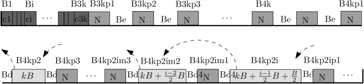
Figure 5: The basic idea for the proof of Theorem 2. Modules are not drawn to scale; in particular, modules of size $N=kB+1+rB/2$ (gray) for an appropriately large integer $r$ are very large, so they can never be moved. The modules $M_{1},\ldots,M_{3k}$ encode an instance of 3-Partition. Module $M_{4k+2}$ of size $k\cdot B$ can be moved if and only if these first $3k$ modules (dark-gray) can be moved to the first $k$ free spaces of size $B$. Only in this case, for $i=2,\ldots,r$, the modules $M_{4k+2i}$ (light-gray) fit exactly between $M_{4k+2i-3}$ and $M_{4k+2i-1}$, increasing the size of the largest free interval by $B/2$ with every move.

Note that the number of modules is $n=5k+4r+1$ and $\max\{\log f_{\mathrm{max}},\log b_{\mathrm{max}}\}=\log b_{\mathrm{max}}$. We claim that $f_{\mathrm{alg}}\geq kB$ if and only if the answer to the 3-Partition instance is “yes”.

If $f_{\mathrm{alg}}\geq kB$, consider the situation in which the first free space of size $kB$ occurs. Because none of the modules $M_{3k+1},\ldots,M_{4k+2r+1}$ could be moved so far, and because the modules $M_{1},\ldots,M_{3k}$ are larger than $B/4$, the only way to create a free space of size $kB$ is to place the first $3k$ modules in the $k$ free spaces of size $B$. This implies a solution to the 3-Partition instance.

If $f_{\mathrm{alg}}<kB$, we show that the instance of 3-Partition cannot be solved. If $f_{\mathrm{alg}}<kB$, then

$$f_{\mathrm{opt}}\leq\alpha\cdot f_{\mathrm{alg}}+\beta<kB\cdot C\cdot(n\log b_{\mathrm{max}})^{1-\varepsilon}+\beta\;,$$

for some constant $C$. The total free space has size $f=kB+rB/2$. Because $n=5k+4r+1$, $b_{\mathrm{max}}=N=kB+1+rB/2$ and $k$, $B$, $C$, and $\beta$ are constant a straightforward computation shows that

$$f_{\mathrm{opt}}<kB\cdot C\cdot\left[(5k+4r+1)\log(kB+1+\frac{rB}{2})\right]^{1-\varepsilon}+\beta\leq kB+\frac{rB}{2}=f\;,$$

for large $r$ (i.e., we choose $r$ such that the second inequality holds). Hence, a free space of size $kB+rB/2$ cannot be constructed.

Conversely, a solution to the 3-Partition instance allows the construction of a free space of size $kB+rB/2$ as follows. The first $3k$ modules are moved to the $k$ free spaces of size $B$. Now, $M_{4k+2}$ is moved to the free space of size $kB$ and then, one after the other, $M_{4k+2i}$ is moved between the modules $M_{4k+2i-3}$ and $M_{4k+2i-1}$, for $i=2,\ldots,r$.

Thus, we can conclude that the existence of a polynomial-time approximation method for the MDP can be used to decide the feasibility of 3-Partition instances, i.e., implies P=NP. ∎

5 Moderate Density

The number of modules, $n$, their sizes, and the amount of free space on the reconfigurable area are highly dependent on the application to be executed and, furthermore, may also vary enormously during the execution of the application on a reconfigurable device. Initially or at some later point in time, only a portion of the reconfigurable device may be used. For a rather moderate density, we conceived an efficient defragmentation routine. We consider a special case in which the homogeneous MDP can be solved with linear computing time in at most $2n$ moves. We define the density of an array, $L$, of length $\ell$ to be $\delta:=\frac{1}{\ell}\sum_{i=1}^{n}m_{i}$. We show that if the density is bound by $\frac{1}{2}(1-$ the fraction of the total area occupied by the largest module), i.e.,

$$\delta\leq\frac{1}{2}-\frac{1}{2}\cdot\frac{\max_{i=1,\ldots,n}\{m_{i}\}}{\ell}$$ (1)

the total free space can always be connected with $2n$ steps by Algorithm 1. The idea of the Algorithm 1 is to start with the leftmost module, and shift all modules as far as possible to the left, one after the other. In the second loop, we start with the rightmost module and shift modules as far as possible to the right, one after the other. As it turns out, this results in one connected free space. (Note that in some cases, a single round of shifts is sufficient, which can easily be detected; however, two rounds may be necessary if the initial configuration has small free intervals on the left.)

Input: A array $L$ with $n$ modules $M_{1},\ldots,M_{n}$ such that (1) is fulfilled.

Output: A placement of $M_{1},\ldots,M_{n}$ such that there is only one free interval at the left end of $L$.

for $i=1$ to $n$ do  Shift $M_{i}$ to the left as far as possible. end for $i=n$ to $1$ do  Shift $M_{i}$ to the right as far as possible. end

Algorithm 1 LeftRightShift

5

5

5

5

5

For proving correctness of Algorithm 1, we need the following two observations. Both follow immediately from the definition of density and from (1); in the following, $f_{i}$ denotes the size of free intervals $F_{i}$.

$$\sum_{i=1}^{k}f_{i}\geq\frac{l}{2}+\frac{1}{2}\cdot\max_{i=1,\ldots,n}\{m_{i}\}$$ (2)

$$\delta<\frac{1}{2}\;\;\mbox{and therefore}\;\;\sum_{i=1}^{n}m_{i}<\sum_{j=1}^{k}f_{j}$$ (3)

Theorem 3.

Algorithm 1 connects the total free space with at most $2n$ moves and uses $O(n)$ computing time.

Proof.

The number of shifts and the computing time are obvious. We will show that at the end of the first loop, the rightmost free interval is greater than any module and therefore all modules can be shifted to the right in the second loop.

Let $F_{1},\ldots,F_{k}$ denote the free intervals in $L$ at the end of the first loop. Then every $F_{i}$, $i\in\{1,\ldots,k-1\}$ is bounded to the right by a module $M_{j}$ with $m_{j}>f_{i}$ (otherwise $m_{j}$ could be shifted). If this holds for $F_{k}$ as well, we can conclude that $\sum_{i=1}^{k}f_{i}<\sum_{i=1}^{n}m_{i}$, which contradicts (3). Hence, there is no module to the right of $F_{k}$, and we get with $m^{\star}=\max_{1,\ldots,n}\{m_{i}\}$

$$\frac{l}{2}+\frac{1}{2}m^{\star}\stackrel{{\scriptstyle(\ref{eq:lowden3})}}{{\leq}}\sum_{i=1}^{k}f_{i}<\sum_{i=1}^{n}m_{i}+f_{k}\stackrel{{\scriptstyle(\ref{eq:lowden2})}}{{\leq}}\frac{l}{2}-\frac{1}{2}m^{\star}+f_{k}$$

implying $m^{\star}<f_{k}$. ∎

6 A Quadratic Lower Bound

As a consequence of the hardness and inapproximability results we focus on developing heuristic approaches for the MDP. In this section, we bound the number of steps needed by any algorithm that constructs a maximum free interval, even in the homogeneous version. In the next sections, we state a heuristic and give experimental results.

Theorem 4.

There is an instance of the maximum defragmentation problem such that any algorithm needs at least $\Omega(n^{2})$ steps to solve it.

Proof.

We construct the instance in the following way. For an even number $n$, we place $n$ modules, indexed from left to right by $1,\ldots,n$. The sizes of the modules are $m_{j}=m_{n+1-j}=n+2-2j$ for $1\leq j\leq\frac{n}{2}$. $M_{1}$ has a free interval of size $1$ to its left and $M_{n}$ has a free interval of size $1$ to its right. In addition, every pair of consecutive modules is separated by a free interval of size one, except for the pair $M_{\frac{n}{2}}$ and $M_{\frac{n}{2}+1}$, which is separated by a distance of two. In this initial configuration we denote the free intervals by $F_{1},\ldots,F_{n+1}$, and their sizes by $f_{1},\ldots,f_{n+1}$. Fig. 6 shows an example for $n=8$.

Figure 6: The instance for $n=8$.

The following properties of this instance are essential for the rest of the proof:

• The module sizes $m_{j}=m_{n+1-j}=n+2-2j$, $1\leq j\leq\frac{n}{2}$, are even.

• $m_{j}=m_{n+1-j}=\sum_{i=j+1}^{n+1-j}f_{i}$ holds for any pair $M_{j}$, $M_{n+1-j}$ (i.e., the total free interval between two modules of equal size is equal to the modules’ sizes).

• Every module has to be moved at least once (because of the small free intervals at the left and right end of $L$).

• For $i<j\leq\frac{n}{2}$, we have $m_{i}=m_{n+1-i}\geq m_{n+1-j}=m_{j}$; in particular, this means that the pair $M_{i}$, $M_{n+1-i}$ can be moved only if $M_{j}$, $M_{n+1-j}$ can be moved.

In the beginning, only the modules $M_{\frac{n}{2}}$ and $M_{\frac{n}{2}+1}$ with $m_{\frac{n}{2}}=m_{\frac{n}{2}+1}=2$ can be moved. Using three moves, a free interval of size four can be constructed. Note that both modules have to be moved and that there can be a free interval of size four only if there is exactly one free interval between $M_{\frac{n}{2}-1}$ and $M_{\frac{n}{2}+2}$. Now we show by induction for $j$ from $\frac{n}{2}$ to $1$ that

• at least $n-2j+2$ steps are necessary to make a pair $M_{j-1}$, $M_{n+1-(j-1)}$ movable after the pair $M_{j}$, $M_{n+1-j}$ became movable and

• in the situation in which $M_{j-1}$, $M_{n+1-(j-1)}$ become movable, there is exactly one free interval between these two modules.

Both properties clearly hold for $j=\frac{n}{2}$ and we assume that $M_{j}$ and $M_{n+1-j}$ for $1\leq j<\frac{n}{2}$ became movable (for the first time) by the last step.

By part (b) of the induction hypothesis, the modules and free intervals in the area between $M_{j-1}$ and $M_{n+1-j}$ are currently arranged in the following order, described from left to right: a free interval of size one, a sequence of modules, a free interval of size $m_{j}$, a sequence of modules, and a free interval of size one (see Fig. 7). The modules in the rest of $L$ are still in their initial position (otherwise $M_{j}$ and $M_{n+1-j}$ could have been moved earlier because of (iv)).

Figure 7: The situation when $M_{j}$ and $M_{n+1-j}$ can be moved for the first time.

Property (b) is a straightforward implication of (ii) and we show that (a) holds as well. Suppose for a contradiction that $M_{j-1}$ and $M_{n+2-j}$ can be made movable without shifting or “jumping” a module $M_{k}$ with $j\leq k\leq n+1-j$, i.e., without moving a modules that lies between $M_{j-1}$ and $M_{n+2-j}$). We assume w.l.o.g. that $M_{k}$ is in the same sequence as $M_{j}$. Thus, the distance from $M_{k}$’s left boundary to the right boundary of $M_{j-1}$ can be calculated as the sum of the sizes of modules lying on the left side of $M_{k}$ plus one. By (i), this is an odd number. The same holds for the distance from $M_{k}$’s right boundary to the left boundary of $M_{n+2-j}$. Again using (i), this implies that none of these intervals can completely be filled with other modules. Hence, by (ii), $M_{j-1}$ and $M_{n+2-j}$ can never be moved without moving $M_{k}$. There are $n-j+2-j-1+1=n-2j+2$ modules initially placed between $M_{j-1}$ and $M_{n+2-j}$ and each of them has to be moved.

Altogether, this implies a lower bound of $\sum_{j=1}^{\frac{n}{2}}(n-2j+2)=\frac{n^{2}}{4}+\frac{3n}{2}$ on the total number of steps. ∎

7 A Heuristic Method

For runtime defragmentation, we propose a tabu search with a tabu list of length $\frac{n}{2}$, see Algorithm 2. In every iteration, all homogeneous modules $M_{i}$ are moved to the left end and to the right end of the free intervals that are greater than or equal to $m_{i}$. All inhomogeneous modules are moved to any feasible position. Each move is evaluated by a fitness function that divides the size of the maximal free interval by the number of free slots. The move yielding the configuration with the highest fitness is chosen. Ties are broken by choosing the first one. The resulting configuration is added to the tabu list.

If the current solution is the best one found so far, it is stored. The heuristic ends if either a fitness of $1.0$ (i.e., optimality) is achieved or $2n^{2}$ iterations have been performed. As seen above, there are instances for which $\Omega(n^{2})$ moves are necessary. Moreover, we conjecture that the number of necessary moves is in $\Theta(n^{2})$.

counter := 0;

tabulist := {};

maxfitness := 0.0;

while (counter $\leq 2n^{2}$) and (maxfitness $<1.0$) do foreach module $M_{i}$ in the array do storedfitness := 0.0 if $M_{i}$ is homogeneous then foreach free interval $F_{j}$ do move $M_{i}$ to the left end of $F_{j}$ evaluate move move $M_{i}$ to the right end of $F_{j}$ evaluate move move $M_{i}$ back to its original position end foreach else foreach position $P$ for $M_{i}$ that is feasible and not blocked by another module do move $M_{i}$ to $P$ evaluate move move $M_{i}$ back to its original position end foreach end if if storedfitness $>$ maxfitness then apply storedmove store storedmove in tabulist maxfitness := storedfitness end if end foreach counter++ end while Procedure evaluate move: if move is not stored in tabulist thisfitness $:=$ size of the maximal free interval / number of free slots if thisfitness $>$ storedfitness then store move in storedmove storedfitness := thisfitness end if end if

Algorithm 2 Tabu Search

3

3

3

8 Experimental Results

8.1 Compacting an FPGA

We performed a series of experiments for defragmentation based on scenarios of FPGAs with and without heterogeneities and different densities (i.e., different ratios of occupied space compared to unoccupied space). Fig. 8 shows the results for two FPGAs, both having 94 slots. The first FPGA does not contain any heterogeneities, while the second one is an FPGA with heterogeneities at positions 3, 24, 45, 50, 71 and 82. Moreover, we compared our heuristic to a simple greedy approach that moves every module to the most promising position (i.e., to the position for which the ratio of the size of the maximal free interval and the size of the total free space is maximal).

Generating the input was done in two steps, depending on the size of the maximal free interval $F^{\star}$. In the first step the module size is chosen with equal probability from the set {$1,\ldots,f^{\star}$}. This ensures that the modules can be inserted. The exact position is chosen again with equal probability among all feasible positions. If the interval occupied by the module contains an heterogeneity, this heterogeneity is assigned to the corresponding position of the module. The size of the first module is shrunk by a factor of $0.6$ in order to ensure that it can be moved.

For the density ranging from $0.3$ to $0.9$ with steps of size $0.05$, we performed 100 runs of the tabu search and the greedy strategy for each value and took the average value of the number of free intervals and the size of the maximal free interval. The results are shown in Fig. 8. The diagrams show the size of the maximal free interval (top row) of the array and the number of free spaces (bottom row) before and after the defragmentation. In the array with no heterogeneities (left column), there is an improvement of up to 40%. On the FPGA (right column) the size of any maximal free interval is limited to $20$ slots due to the heterogeneities. For a density of less than $\frac{1}{2}$, the tabu search achieves this upper bound for almost all instances. For larger densities, it achieves an improvement of approximately 35%.

The change in the number of free intervals before and after defragmentation is displayed in the right charts of Fig. 8. In the array with no heterogeneities there is an increase of 50%. For the FPGA there is almost no improvement for low densities (less than $\frac{1}{2}$) and an improvement of approximately 25% for larger ones.

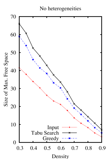
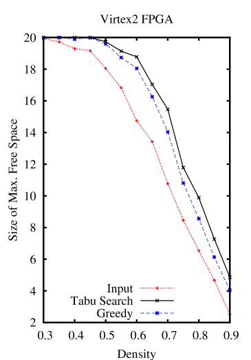
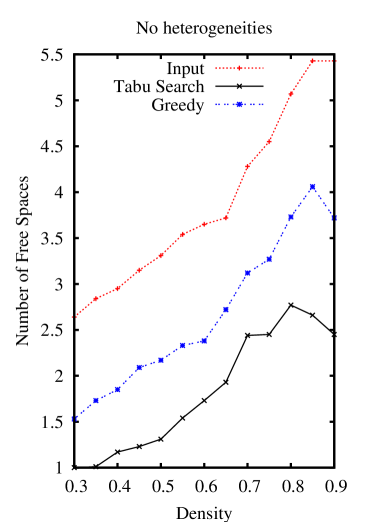
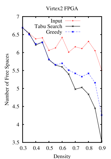
Figure 8: Averages over 100 runs. (Top left) Size of the maximal free interval before and after defragmentation, using our heuristic and a simple greedy approach in an array with no heterogeneities.
(Top right) Size of the maximal free interval before and after defragmentation of the FPGA.
(Bottom left) Number of free intervals before and after defragmentation in an array with no heterogeneities.
(Bottom right) Number of free intervals before and after defragmentation of the FPGA.

8.2 Case Study

In this section, a case study is given that demonstrates the efficiency of the proposed techniques and how they can be applied to a real-world scenario. We assume a dynamically partially reconfigurable device, whose reconfigurable area is separated into $94$ columns, also called slots. Modeling typical FPGAs, some of these slots contain no logic resources, but a heterogeneities such as BlockRAMs. This setting is illustrated in Figure 9.

Furthermore, assume that one or multiple applications with a collection of modules are executed on this device; e.g., these could a video processing and a number cruncher application whose current state can rather easily be saved and restored at a different position on the reconfigurable device with moderate costs. During the execution of the applications, different modules finish and are removed, while new modules need to be placed. Thus, the free space on the reconfigurable device can be scattered over the whole reconfigurable area. This situation is illustrated in the upper part of Figure 10.

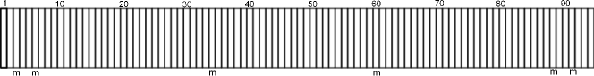
Figure 9: Initial state in example scenario. The reconfigurable device consists of $94$ partially reconfigurable, empty slots. Those containing a heterogeneity, such as BlockRAMs, are marked below with an “m”.

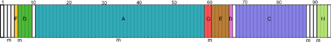
Figure 10: (Top) Fragmented state in example scenario. Free space is scattered over the whole reconfigurable area. (Bottom) Free space after defragmentation with greedy approach.

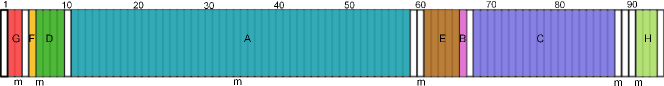
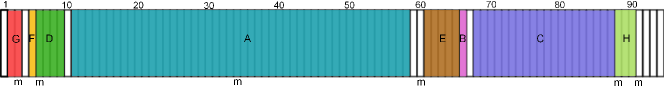
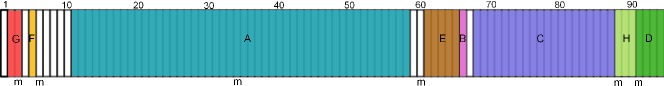
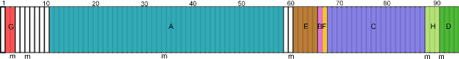
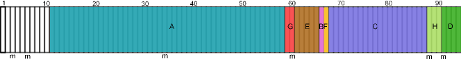
Figure 11: Tabu-search algorithm: defragmentation in four move steps (shown from top to bottom).

The fragmented free space on the reconfigurable area is a common, unavoidable scenario, for which our proposed defragmentation techniques represent an applicable and efficient solution. Our first approach, the greedy algorithm, selects in each setting a step that optimizes the resulting maximal contiguous free space. Based on the state of the example in the upper part of Figure 10, the greedy algorithm moves the module ”G” to position $59$. Thus, a biggest free space is achieved within a single move. The heterogeneity requirements of module ”G” are fulfilled at the time at this position: at position $60$, BlockRAMs are provided for the right part of the module. Afterwards, no single move that provides an improvement on the maximum free contiguous space is possible. Thus, the greedy algorithm terminates. Note that the evaluation of each possible step in the algorithm checks the maximal free space by taking into account all contiguous free slots, no matter if they contain heterogeneities or not.

In our second approach, the maximum free contiguous space is optimized using tabu search, see Figure 11. Based on the state of the same example, module ”H” is relocated to slot position $88$. This step yields a maximal, contiguous free space of four slots including a single BlockRAM heterogeneity slot. In a second step, module ”D” is moved to slot $91$, where module ”H” was located before. Thus, a new maximal free space is created starting at slot $6$ up to $10$. All other steps would have created a free contiguous space with a size less than $5$ slots. Further, this is also the only position to which module ”D” can be moved, due to its heterogeneity constraints. In a third step, module ”F” is moved to the single empty slot without BlockRAMs between module ”B” and module ”C”. In a next step, module ”G” can be either moved to slot position $6$ or to slot position $59$; both satisfy its heterogeneity demands. Finally, it is moved to the latter position, because this results in a maximal free space of $10$ slots. It is also possible that multiple single steps offer the same increase in contiguous free space; in our current implementation, one single move is selected randomly.

When the greedy algorithm is applied to the example input, a contiguous free space of four slots is achieved. In contrast, the tabu search merges all free space and yields one single contiguous block of free space of size $10$. This shows the usefulness of defragmentation techniques, and the importance of the corresponding strategy. Similar scenarios of scattered empty space and heterogeneities on the reconfigurable device are common when executing modules. New modules with big area requirements must unnecessarily be delayed without defragmentation steps, which can be avoided with appropriate defragmentation strategies. How far different strategies can deviate is shown by comparing the results of the greedy and the tabu-search approach for this example.

8.3 Makespan

Figure 12: Comparison of makespans for schedules using tabu search, greedy, and no fragmentation for an array of size $\ell=200$. The average module size is fixed to 10, 50, and 150 columns, the average duration time ranges from 1 to 400 time units. The $y$-axis shows the total makespan in time units.

Figure 13: Comparison of makespans for schedules using tabu search, greedy, and no fragmentation for an array of size $\ell=200$. The average module size is fixed to 10, 50, and 100 columns, the average duration time ranges from 600 to 3000 time units. The $y$-axis shows the total makespan in time units.

We also simulated the impact on the total makespan (i.e., the total execution time) by randomly generating sequences of modules. A sequence consists of 200 modules, for each module we chose size and duration randomly using different distributions. Fig. 12 and Fig. 13 show examples in which the size was chosen by normal distribution and duration according to an exponential distribution. We used the exponential distribution for the duration time, because this distribution models typical life times [2]. We normalized the duration times, i.e., we define the time to write a single FPGA column to be 1 time unit.

For each pair of size and duration values, we shuffled 100 sequences and calculated their makespan by simulating the processing of a sequence using tabu search, greedy, and no defragmentation. More precisely, we successively place the modules into an array that represents the FPGA. If we cannot place a module, because there is no sufficient free space, either the module has to wait (no defragmentation) or we perform the tabu search or the greedy strategy to compact the FPGA. After the duration time for a module elapsed, it is removed from the array. Our simulation takes the times needed to place or move a module into account; the duration time is prolonged accordingly.

It turned out that it pays off to use defragmentation for larger modules or larger duration times. Small modules with small duration time enter and leave the system so quickly that there is no need for defragmentation, see Fig. 12(left) up to an average duration of 50 time units. At smaller module sizes and execution times, greedy’s shorter running time beats the effectiveness of the tabu search (Fig. 12(left) from 75 to 350). However, as the average module size (as a fraction of the total area) or execution length increases, the more compact solution provided by the tabu search provides a better overall execution time, even with increased overhead (Fig. 12(left) from 350 and Fig. 13(left)). For modules of medium size (compared to the size of the FPGA), the tabu search decreases the total makespan (Fig. 12(middle) and Fig. 13(middle)). If the average size of a module approaches or even exceeds half the size of the FPGA, the benefit of compaction disappears (Fig. 12(right) and Fig. 13(right)). Note that in this case, compaction is often not even possible because the modules are too large to be moved.

9 Conclusion

In this paper, we presented a new approach for defragmenting the module layout on a dynamically reconfigurable device, for example a FPGA, in a seamless fashion. As the reconfiguration costs continuously decrease with each new generation of reconfigurable devices and a number of techniques for task preemption and relocation at a different positions are conceived (see Koch et al. [18] for a comparison), task relocation at runtime becomes a new opportunity for improving the performance and efficiency of reconfigurable devices. However, this also poses new challenges, because defragmentation methods developed so far cannot be applied to reconfigurable devices, as they do not take into account their special characteristics. For example, many reconfigurable devices have heterogeneities on their reconfigurable area, such as memory blocks, DSPs, and CPUs. We presented different defragmentation strategies to relocate running modules and achieve a contiguous free space of maximum size.

The presented experiments show in average an increase in the maximal free space by $30\%$ when applying our defragmentation techniques to FPGAs with heterogeneities; on some inputs an increase up to $200\%$ is observed. This additional free space allows earlier execution of later modules, so the total execution time is reduced. This shows that it pays off to prefer a sophisticated heuristic for defragmentation (e.g., tabu search) over a simple heuristic (i.e., greedy), or over no defragmentation at all; provided that the execution times and module sizes are not too extreme (i.e., too large or too small compared to the size of the FPGA).

Obviously, improved algorithmic results can lead to further improvements. One of the possible extensions considers a more controlled overall placement of modules, instead of simply fixing fragmentation. As the necessary algorithmic methods are more involved, we leave this to future work.

References

- [1] T. Becker, W. Luk, and P. Y. Cheung. Enhancing relocatability of partial bitstreams for run-time reconfiguration. In Proc. 15th Annu. Sympos. Field-Programm. Custom Comput. Mach., pages 35–44, 2007.
- [2] K. Behnen and G. Neuhaus. Grundkurs Stochastik. B.G.Teubner-Verlag, 3nd edition, 1995.
- [3] M. A. Bender, E. D. Demaine, and M. Farach-Colton. Cache-oblivious B-trees. SIAM J. Comput., 35:341–358, 2005.
- [4] M. A. Bender, J. T. Fineman, S. Gilbert, and B. C. Kuszmaul. Concurrent cache-oblivious B-trees. In Proc. 17th Annu. ACM Sympos. Parallel. Algor. Architect., pages 228–237, 2005.
- [5] G. Bromley. Memory fragmentation in buddy methods for dynamic storage allocation. Acta Inform., 14:107–117, 1980.
- [6] C. Claus, R. Ahmed, F. Altenried, and W. Stechele. Towards rapid dynamic partial reconfiguration in video-based driver assistance systems. In ARC, pages 55–67, 2010.
- [7] K. Compton, Z. Li, J. Cooley, S. Knol, and S. Hauck. Configuration relocation and defragmentation for run-time reconfigurable systems. IEEE Transact. VLSI, 10:209–220, 2002.
- [8] S. P. Fekete, T. Kamphans, N. Schweer, C. Tessars, J. C. van der Veen, J. Angermeier, D. Koch, and J. Teich. No-break dynamic defragmentation of reconfigurable devices. In Proc. Internat. Conf. Field Program. Logic Appl., pages 113–118, 2008.
- [9] M. R. Garey and D. S. Johnson. Computers and intractability; a guide to the theory of NP-completeness. W.H. Freeman, 1979.
- [10] M. G. Gericota, G. R. Alves, M. L. Silva, and J. M. Ferreira. Run-time defragmentation for dynamically reconfigurable hardware. New Algorithms, Architectures and Applications for Reconfigurable Computing, 2005.
- [11] J. Hagemeyer, B. Kettelhoit, M. Koester, and M. Porrmann. Design of homogeneous communication infrastructures for partially reconfigurable FPGAs. In Proc. Internat. Conf. Eng. Reconf. Syst. Algor., 2007.
- [12] J. A. Hinds. An algorithm for locating adjacent storage blocks in the buddy system. Commun. ACM, 18:221–222, 1975.
- [13] D. S. Hirschberg. A class of dynamic memory allocation algorithms. Commun. ACM, 16:615–618, 1973.
- [14] K. C. Knowlton. A fast storage allocator. Commun. ACM, 8:623–625, 1965.
- [15] D. E. Knuth. The Art of Computer Programming: Fundamental Algorithms, volume 1. Addison Wesley, Reading, Massachusetts, 3rd edition, June 1997.
- [16] D. Koch, A. Ahmadinia, C. Bobda, and H. Kalte. FPGA architecture extensions for preemptive multitasking and hardware defragmentation. In Proc. IEEE Internat. Conf. Field-Programmable Technology, pages 433–436, Brisbane, Australia, 2004.
- [17] D. Koch, C. Beckhoff, and J. Teich. ReCoBusBuilder — A novel tool and technique to build static and dynamically reconfigurable systems for FPGAs. In Proc. 18th Internat. Conf. Field Programm. Logic Appl., pages 119–124, 2008.
- [18] D. Koch, C. Haubelt, and J. Teich. Efficient hardware checkpointing—concepts, overhead analysis, and implementation. In Proc. 15th ACM/SIGDA Internat. Sympos. Field-Programm. Gate Arrays, pages 188–196, Monterey, California, USA, 2007. ACM.
- [19] D. Koch, C. Haubelt, and J. Teich. Efficient reconfigurable on-chip buses for FPGAs. In Proc. 16th Annu. IEEE Sympos. Field-Programm. Custom Comput. Mach., Palo Alto, CA, USA, Apr. 2008.
- [20] M. Koester, H. Kalte, M. Porrmann, and U. Ruckert. Defragmentation algorithms for partially reconfigurable hardware. Internat. Federation for Information Processing Publications (Ifip), 240:41, 2007.
- [21] I. Kuon and J. Rose. Measuring the gap between FPGAs and ASICs. IEEE Trans. CAD Integr. Circuits Systems, 26:203–215, Feb. 2007.
- [22] P. Lysaght, B. Blodget, J. Mason, J. Young, and B. Bridgford. Invited paper: Enhanced architecture, design methodologies and CAD tools for dynamic reconfiguration of Xilinx FPGAs. In Proc. 16th Internat. Conf. Field Programm. Logic Appl., pages 1–6, Aug 2006.
- [23] K. K. Shen and J. L. Peterson. A weighted buddy method for dynamic storage allocation. Commun. ACM, 17:558–562, 1974.
- [24] P. R. Wilson, M. S. Johnstone, M. Neely, and D. Boles. Dynamic storage allocation: A survey and critical review. In H. Baker, editor, Proceedings of International Workshop on Memory Management, volume 986 of Lecture Notes in Computer Science, Kinross, Scotland, Sept. 1995. Springer-Verlag.