Speeding up evolutionary search by small fitness fluctuations

Abstract

We consider a fixed size population that undergoes an evolutionary adaptation in the weak mutuation rate limit, which we model as a biased Langevin process in the genotype space. We show analytically and numerically that, if the fitness landscape has a small highly epistatic (rough) and time-varying component, then the population genotype exhibits a high effective diffusion in the genotype space and is able to escape local fitness minima with a large probability. We argue that our principal finding that even very small time-dependent fluctuations of fitness can substantially speed up evolution is valid for a wide class of models.

1 Introduction

Organisms adapt to their environment by sequential fixation of beneficial mutations. This process is often visualized as motion of a population (specified by multi-dimensional genomic variables corresponding to the dominant genotype in the population) in the fitness landscape, where the height of the landscape corresponds to the reproductive fitness of an average individual in the population Wright1932 . Fitness landscapes are believed to be rough with many local maxima, and a population may get stuck in one, so that every plausible mutation is deleterious. In such cases adaptation to a global fitness maximum requires the fixation of deleterious mutations, which is rare. Even when there is a path of only neutral or weakly selective mutations to the global optimum, it may be difficult to find it, and navigating such paths can be slow due to the low fixation probability ($\approx 1/N$ for a population of $N$ individuals for a neutral mutation Kimura1962 ).

It has been recognized that temporal fluctuations in the fitness landscape can drive the population out of a local fitness maximum. For example, the maximum of fitness at one time may be on a fitness slope at another time, allowing the population to leave the area. Such connections between the fluctuating selective pressure, the population size, and the population-genetics dynamics have been studied extensively Gillespie1994 ; Mustonen2008 , starting with the introduction of the concept of adaptive topography by Wright Wright1932 . More recently the evolutionary dynamics of density regulated populations in fluctuating environments have been elucidated in more ecologically realistic models Heckel1980 ; MacArthur2001 ; Lande2009 , bridging the gap between the classical population dynamics Namba1984 ; Cushing1986 and the population genetics models.

In a recent pioneering numerical evolution experiment Kashtan2007 , these ideas were further developed to show that certain type of fluctuating environmental pressures speed up evolution many times in a particular model. However, it remains unknown to what extent these results generalize. Is the speedup a general property? How does it depend on the spatiotemporal structure of the fluctuating environment? Can a population escape any local maximum? How does the motion in the genotype space depend on time? Do fitness fluctuations have to be dramatic, as in Ref. Kashtan2007 , or can small fluctuations still speed the evolution up?

In this article, we answer some of these questions in the context of a model of evolutionary dynamics that is simple enough to allow a thorough analytical and numerical treatment, but is at the same time general enough so that at least some of our predictions hold for a wide class of evolutionary models. We consider the limit of a weak mutation rate, when the time scales are well separated. The time between successive mutations is slower that the typical fixation time, and the characteristic time scale of the fitness landscape changes is the longest. Further, we assume a constant population size, so that the evolutionary dynamics depends only on the relative fitness differences between the genotypes. We consider adaptation in a highly epistatic genotypic space, such that the evolution takes place on a one dimensional pathway with large, local fitness differences. Under these assumptions, we show that the evolutionary search can be sped up substantially when only a small component of the fitness landscape undergoes temporal variations.

2 The model

Our model of a fluctuating environment is based on an overdamped Langevin particle in a potential. The position $x$ is some generalized coordinate that describes the dominant genotype in the population, and hence a change in $x$ is a fixation event. This genotype changes with the velocity given by

$$\frac{dx}{dt}=-\frac{1}{\gamma}\frac{\partial U(x,t)}{\partial x}+\eta,$$ (1)

where $U$ is the potential, $\gamma$ is the friction, $\eta$ is a white Gaussian noise with the variance $2D$, where $D$ is the intrinsic diffusivity. Notice that in the usual physics language, the process will minimize the potential so that $U$ is the negative fitness.

Motion to minimize $U$ represents fixation of beneficial mutations, while Langevin noise allows low probability fixation of neutral and deleterious mutations. The first phenomenon is called natural selection/drift in evolutionary/physics languages, and the second is unfortunately referred to as drift/diffusion, respectively. To avoid confusion, in the remainder of the article we use the physics terminology.

We write the potential as

$$U(x,t)=U_{0}(x)+\Phi(x)S(t),$$ (2)

and we focus on the following range of parameters:

$${\rm var}\,S(t)\sim 1,$$ (3)

$$\max[\Phi(x)]-\min[\Phi(x)]\ll\max[U_{0}(x)]-\min[U_{0}(x)]$$ (4)

This models the emergence of novel functions in a population. Namely, the fitness is largely independent of time, as described by $U_{0}$. However, small temporal changes in fitness are allowed. For example, acquiring an enzyme that can metabolize a certain chemical is generally advantageous if the chemical is present, but somewhat deleterious if it is absent, so that the investment into production of the enzyme cannot recovered. We model this by adding the small fitness component $\Phi(x)$ that fluctuates as $S(t)$, representing, for example, changes in the availability of the metabolite due to seasonal or geological variations. Finally, we choose to separate the global, almost non-epistatic, fitness from the local, possibly highly-epistatic (but small) effects by making the gradient of $U_{0}$ smaller than that of $\Phi$, even though the scale of $\Phi$ itself is smaller than that of $U_{0}$.

With the conditions above, we can redefine $U_{0}$, $\Phi$, and $S$ without much loss of generality, so that $\langle S\rangle_{t}=0$. We then consider the simplest form of $\Phi(x)$ and $S(t)$ that satisfy these conditions, and we will discuss how our results generalize to other forms of the functions in Section 5. Namely, we choose $\Phi$ to be a zero-mean periodic saw-tooth potential, and $S$ to be a zero-mean periodic telegraph signal. These considerations allow us to write near a particular point $x$ in the genotype space

$$\frac{1}{\gamma}\frac{\partial U}{\partial x}=-v+\phi(x)s(t),$$ (5)

$$\phi(x)\equiv\frac{h}{L}\times{\rm sign}\left[\sin\frac{\pi x}{L}\right],$$ (6)

$$s(t)\equiv{\rm sign}\left[\sin\frac{\pi t}{T}\right],$$ (7)

where $v$ is the intrinsic drift or bias, defined as positive for the drift to the right, see Fig. 1. We always assume that $|h|/L>|v|$, so that the fluctuating component of the potential can actually create local maxima and minima on top of the global landscape $U_{0}(x)$. In what follows we denote by $T$ the time between subsequent potential flips (the half-period of the fluctuations), and $L$ is half of the spatial period.

This model is similar to various stochastic ratchets considered in the literature Magnasco1993 ; Tarlie1998 ; Dubkov2005 ; Sinitsyn2007 . Thus, intuitively, the question of whether the fitness fluctuations can speed up the evolutionary search is a question similar to whether a rectified or a high-variance motion can appear due to ratcheting.

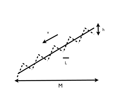
Figure 1: The potential $U(x,t)$ at a fixed time. An oscillatory, symmetric, sawtooth perturbation is added on top of the average linear potential that creates a drift velocity of $v$.

2.1 Rescaling of the equation of motion

Using the choices above, we can rewrite the equation of motion, Eq. (1) as

$$\frac{dx}{dt}=\left[-\phi(x)s(t)+v\right]+\sqrt{2D}\eta.$$ (8)

where $\eta$ is a Gaussian white noise of unit variance. In Eq. (8), the dynamics explicitly depends on five different parameters $L$, $T$, $v$, $h$, and $D$. Nevertheless, by rescaling the time, the space, and the potential as $x/L\to x$, $t/T\to t$, $\frac{L}{h}\phi\to\phi$, $\frac{L}{h}v\to v$, we can reduce the number of parameters to only three: the ratio of the typical diffusion time over half the spatial period to half of the temporal period, $\omega=\frac{L^{2}}{2DT}$, the height of the fluctuating barriers in diffusivity (temperature) units, $\beta=\frac{h}{D}$, and the ratio between the slope of the average, large scale potential to the slope of the fluctuating perturbation, $v$. In physical terms, $\omega$ represents the diffusion time over the distance $L$: if $\omega$ is large, the particle has time to explore the entire valley of $\phi$ before the potential flips. Further, $\beta$ measures the difficulty of crossing the peaks by diffusion. Finally, the condition that the perturbation induces local optima is $|v|<1$

Using the rescaled variables, the dynamics becomes

$$\frac{dx}{dt}=\frac{\beta}{2\omega}\left[-\phi(x)s(t)+v\right]+\sqrt{\frac{1}{\omega}}\eta.$$ (9)

We will use these rescaled variables in the rest of the article, unless noted otherwise. From this equation, it is easy to recover the dynamics in the original, non-scaled units by simple multiplications. In what follows we present simulation results obtained using first order Euler integration scheme of the dynamics defined in rescaled variables, Eq. (9).

3 Fluctuating potentials enhances diffusion and drift

Numerical simulations suggest that the behavior of $x(t)$ at large times is diffusive, and anomalous scaling is not seen Weiss1986 ; Metzler2000 ; Lubelski2008 ; Bel2009 . We can characterize the genotype coordinate motion by an effective drift and a diffusion constant, which depend on the spatial and the temporal periods of the fluctuations and the barrier height. To characterize the enhancement or the suppression of the motion compared to the intrinsic diffusivity and drift, we define

$$r_{D} \equiv\frac{D_{\textrm{eff}}}{D}=\frac{\textrm{var}_{t}(x)}{2t}\frac{L^{2}}{DT}=\frac{\textrm{var}_{t}(x)}{t}\omega,$$ (10)

$$r_{v} \equiv\frac{v_{\textrm{eff}}}{v}=\frac{\langle x(t)\rangle}{t}\frac{L}{vT}=\frac{\langle x(t)\rangle}{t}\frac{2\omega}{v\beta},$$ (11)

where the time-dependent means and variances of the trajectories $x(t)$ are obtained numerically. As seen in the Fig. 2, both the effective drift and the effective diffusion can be enhanced with respect to the intrinsic values, this enhancement having a maximum for fluctuation periods comparable to the average time to travel between two inflection points.

3.1 Building intuition

When $\beta\ll 1$, the sawtooth peaks are very small, and the diffusion has no trouble crossing them. When $\beta$ is larger, the behavior is more interesting. For $\omega\to 0$, the particle has ample time to fall into a minimum of $\phi$ before $s(t)$ flips. Then when the potential flips, the particle can now go either left or right, both with large probabilities, which creates a biased random walk behavior with the effective diffusion coefficient $\approx{L^{2}}/({2T})$, or, equivalently, $r_{D}\approx\omega$, and the system is only weakly sensitive to the value of $v$. The fluctuating potential allows the particle to diffuse against the drift, so that the speed of the evolutionary search is strongly enhanced when the environment oscillates.

For low $\omega$, $r_{D}\approx\omega$ is also small, so the diffusion is suppressed compared to the internal value. However, for $h\gg 1$ and without the changing sign of $s(t)$, the particle would get stuck at a minimum of $\phi$ almost immediately, and the overall diffusion would be, essentially, zero: it is hard to exit a deep potential only well with the help of diffusion. Whether $r_{D}$ is greater or less than 1, the fact that oscillations make it nonzero is our most important finding, suggesting that temporal fluctuations can make fixation of rare-to-fixate mutations a much more common process. Figure 2 demonstrates these findings for different values of $\omega$ and for $\beta=10$ and $v=1/10$.

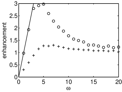
Figure 2: Enhancement of diffusion, $r_{D}=\frac{D_{\rm eff}}{D}$ (circles) and drift, $r_{v}=\frac{v_{\textrm{eff}}}{v}$ (pluses) as a function of the relative flipping frequency $\omega=\frac{L^{2}}{2DT}$, with $\beta=10$ and $v=1/10$. At low $\omega$, the particle has time to reach the minima, and $D_{\rm eff}\approx\frac{L^{2}}{2T}$, or $r_{D}\approx\omega$. Simulations are averaged over 1000 trajectories and 1000 time steps. Solid line indicates $r_{D}=\omega$. Error bars are smaller than the symbols.

When the flipping is fast compared to the diffusion time (large $\omega$ in the Figure), the fluctuating potential ”blurs” together and is effectively zero. The only motion is due to the internal diffusion $D$ and $r_{D}$ goes to one.

3.2 Analytical treatment at $\beta\to\infty$

In the limit $\beta\gg 1$, the peaks are very high, the particle almost never crosses them due to noise, and analytical progress can be made. First consider a particle that starts close to a local minimum $x_{0}$ of the sawtooth. After some time $\sim{D}/{v^{2}}$, which goes to zero as $\beta\rightarrow\infty$, the particle equilibrates near $x_{0}$ with a probability density

$$p(x|x\gtrless x_{0})\propto e^{-(1\mp v)|x|}.$$ (12)

Then the ratio between the probability, $k_{>}$, that a particle is located to the right of $x_{0}$ and will move to the right after the potential flips to the probability, $k_{<}$, that it is to the left of $x_{0}$ and will move to the left is

$$\frac{k_{>}}{k_{<}}=\frac{1-v}{1+v}.$$ (13)

When $s(t)$ changes sign, for a small $D$ the particle then glides down with a constant velocity in its chosen direction, reaching the next minimum to the right ($>$) or to the left ($<$) in

$$\tau_{\gtrless}=\frac{2\omega}{\beta}\frac{1}{(1\mp v)}.$$ (14)

If $\tau_{\gtrless}<1$, then the particle has the time to reach the minimum on either the left or the right hand side (assuming, as always, that the sawtooth actually forms the local minima, i.e., $0<v<1$). Then when the potential flips the next time, the process repeats. This results in a discrete random walk between the extrema of the sawtooth, and (in unscaled variables)

$$D_{\textrm{eff}} =\left[(k_{>}+k_{<})-(k_{>}-k_{<})^{2}\right]\frac{L^{2}}{2T},$$ (15)

$$v_{\textrm{eff}} =\left(k_{>}-k_{<}\right)\frac{L}{T}.$$ (16)

In dimensionless units,

$$r_{D} =\left[(k_{>}+k_{<})-(k_{>}-k_{<})^{2}\right]\omega,$$ (17)

$$r_{v} =\left(k_{>}-k_{<}\right)\frac{2\omega}{v\beta}.$$ (18)

Using Eq. (13) results in:

$$r_{D} =\left(1-v^{2}\right)\omega,$$ (19)

$$r_{v} =\frac{2\omega}{\beta}.$$ (20)

Notably $r_{D}\propto\frac{1}{D}\rightarrow\infty$ when $D\to 0$, but $r_{D}/\beta=D_{\textrm{eff}}/h$ is finite.

In Fig. 3, we compare the analytical results to the numerically estimated $r_{D}$ and $r_{v}$ (here $r_{D}$ is normalized by $\beta/2$). As $\beta\rightarrow\infty$, the agreement is clearly seen for small $\omega$.

When the potential changes faster, and $\tau_{>}>1>\tau_{<}$, the particle fails to make it to the minimum to the right and, after a subsequent flip, always comes back to where it started from. However, it always reaches the left minimum before the flip. When $\tau_{>}>\tau_{<}>1$, it does not reach the left minimum either, but goes the distance $\frac{\beta}{2\omega}(1+v)$ to the left, then reverses and travels $\frac{\beta}{2\omega}(1-v)$ to the right, reverses again and repeats until it reaches the left minimum. After one flip, it moves $\frac{\beta}{2\omega}(1+v)$, after three flips it moves $\frac{\beta}{2\omega}(1+3v)$, and so on. Eventually, when $\beta/(2\omega)[(2n+1)v)+1]>1$, the particle reaches the next minimum. Thus every time $2\omega/(\beta v)$ crosses an odd integer more periods are needed to travel between the nearby extrema, and the diffusive behavior changes, resulting in the discontinuities in Fig. 3. This dynamics can be described by a master equation

$$P_{i}(t+1)=(1-k_{>})P_{i+1}(t-2n)+k_{>}P_{i}(t-1),$$ (21)

where $P_{i}(t)$ stands for being at an extremum $i$ at the end of the flip $t$, and exactly $2n+1$ flips are needed to travel between the $i+1$’th and the $i$’th extrema. Solving this for the drift and the diffusion (see Appendix) gives

$$r_{v} =\frac{1-v}{3+v+2n(1-v)}\frac{2\omega}{v\beta},$$ (22)

$$r_{D} =\frac{8(1-v^{2})}{(3+v+2n(1-v))^{3}}\,\omega.$$ (23)

The analytical results and the numerical simulations verifying them are shown in Fig. 3 with $\omega$ normalized by $\beta/2$.

Figure 3: Effective diffusion (left) and effective drift (right) versus the period of the fluctuations. Notice that $r_{D}$ is normalized by $2/\beta$, and it remains finite even if $D\to 0$ and $\beta\to\infty$. The data are obtained for (in decreasing order of noise strength) $\beta=100$ (squares), $\beta=1000$ (crosses), $\beta=10,000$ (circles), $\beta\rightarrow\infty$ (solid line, analytical result). In the small noise case, the behavior of the diffusing particle is markedly different between Region 1 and Region 2. Region 1 corresponds to small $\omega$ when a particle can always travel between two extrema of the potential, performing an effective biased random walk. Region 2 corresponds to large $\omega$, when the particle spends most of the time traveling between minima but rarely reaching them. Simulations are averaged over 1000 trajectories and 1000 time steps.

4 Fluctuating potential shortens the fitness barrier crossing time

We have shown that the typical diffusive/drift behavior of the system is enhanced by the fluctuating component of the potential. However, what kind of an effect does this enhancement have on the probability of rare, atypical events, such as escape from a suboptimal fitness maximum?

To model a barrier in fitness, we place the overdamped particle in a flipping sawtooth potential and a constant force $v$, and we observe the mean first passage time for the particle to reach an unscaled distance $L\mathcal{M}$, against the drift, with a reflecting boundary at $x=0$, see Fig. 1.

4.1 Fluctuation-activated escape from the minimum is possible even at zero internal diffusion

If during one half period the particle is able to travel between the two extrema, independent of the direction and without the help of the noise, $\tau_{\gtrless}<1$, the probability that the particle travels over multiple periods against the (effective) drift is finite even at a very low noise. As seen in Fig. 4, the escape time over the average barrier in $U_{0}$ depends on the length of the barrier $\mathcal{M}$. In order to understand this dependence, we consider our model in the limit of zero fluctuating potential, which allows us to use an analytical expression for the escape time Redner2001

$$\langle t\rangle_{D}=\frac{\mathcal{M}^{2}}{D}\left[\frac{1}{2Pe}-\frac{1}{4Pe^{2}}\left(1-e^{-2Pe}\right)\right],$$ (24)

where $Pe$ is the Péclet number

$$Pe=\left|\frac{vL{\mathcal{M}}}{2D}\right|.$$ (25)

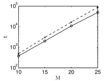
Figure 4: Mean first passage times for crossing a barrier of width $\mathcal{M}$ in our model (simulation, circles) and in a continuous diffusion model with the appropriate effective parameters (crosses). The parameters are $\beta=10$, $\omega=2.5$, $v=-0.1$, and they correspond to the leftmost point in Fig. 3. The exit times from our model are faster than in the diffusion model.

In Fig. 4, we show the simulation results of the exit time for slow fluctuations. We compare the results to what we would have expected under a continuous diffusion with the drift and the diffusion constant given by the values of the effective parameters as obtained in the previous section. We observe that the escape times are well approximated with the “effective” continuous diffusion model. Using a simple discrete space model does not improve the approximation (not shown).

The conclusion is valid even for a very small intrinsic noise $D\rightarrow 0$, which implies that the average time to escape over the global barrier is fluctuation activated (as opposed to noise activated), and is much faster.

4.2 Fluctuations enhance escape even for steep barriers

The qualitative behavior of particle trajectories changes if the fluctuating potential is fast enough such that the particle can only move less than one period in one direction in the absence of the noise. Even though, on average, the variance of the particle position grows linearly, and one can define a proper effective diffusion coefficient, the particle never crosses a barrier against drift in the absence of the intrinsic noise, $\beta\to\infty$. Hence the probability of rare excursions against the effective drift cannot be described using the same effective drift-diffusion model.

Fig. 5 reports results of numerical simulations at different values of the additive noise. The escape time as a function of $\mathcal{M}$ still can be fitted well with a ”drift-diffusion” model, Eq. (24), with a noise dependent effective Péclet number $Pe(\beta)$. We conclude that, for small noises, the effective Péclet number is approximatively inversely proportional to the noise strength (the plot seems to reach a constant for $\beta\to\infty$). This implies that the escape times will become infinite at zero noise. The dependence is consistent with a model without any fluctuating potential, but with some effective parameters. The parameters are such that, with the fluctuations, the escapes are significantly faster. Indeed as shown in Fig. 5, the effective Péclet number, defined as $Pe_{\rm eff}=B\mathcal{M}$, is always smaller than the equivalent quantity in Eq. (24), such that

$$B\ll\left|\frac{vL}{2D}\right|.$$ (26)

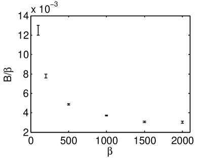
Figure 5: Dependence of the effective Peclet number, $Pe_{\rm eff}=BM$ on the intrinsic noise. We simulate exit times for systems of lengths $\mathcal{M}=1,2,3,4,5$ for different $\beta$. For each dataset with the same $\beta$, we performed a weighted least squares fit for the average escape time of the form $t=A[\exp(B{\cal{M}})-1-B{\cal{M}}]$, fitting for $A$ and $B$. The error bars indicate the confidence bounds of the fits. We show $B/\beta$ versus $\beta$ decreases sublinearly and reaches a constant at $\beta\to\infty$. Thus the mean exit time goes to infinity, but it approaches it much slower than for diffusion with the fluctuating potential, for which $B/\beta=0.1$ for these parameter values, $2\omega/\beta=1$, $v=0.1$.

5 Discussion

Using a one dimensional model of diffusion in the presence of a constant force perturbed by small periodic fluctuations, we have shown that time dependent potentials can significantly speed up the large scale drift, diffusion, and barrier escape times. This conclusion is valid even for a very small intrinsic diffusivity, the long time statistics of the particle trajectories being mainly determined by the properties of the potential fluctuations, but not of the Langevin noise.

Our model is a caricature of evolutionary dynamics in the limit of low mutation rates and constant population sizes. Even in this limit, there are several simplifying assumptions in our model that can be relaxed.

First, the periodicity of the potential time dependence is not crucial. Based on the similarity with Brownian motor models Magnasco1993 ; Tarlie1998 , we expect that our conclusions will still be valid for a nonperiodic $s(t)$: the nonperiodic flipping will mix together and average behaviors from the different regions in Fig. 3. Further, Dubkov et al. Dubkov2005 studied a randomly flipping sawtooth with no drift. Their potential flipped with dichotomous Markovian noise with rate $v$. They found an analytic expression for the diffusion enhancement $r_{D}$: it grows slower than in our model for small $\omega$, and the peak of $r_{D}$ is lower and at larger $\omega$. This is consistent with the averaging over different regions in Fig. 3.

Our model is based on a piecewise linear periodic potential with discontinuous first derivatives (sharp minima and maxima). We expect that our conclusions stay valid as long as the spatially periodic perturbations are sharp enough so that, upon a flip, a particle can leave the vicinity of a maximum in a time much faster than a typical travel time between the extrema. If the potential is not periodic, this will introduce a quenched noise and is likely to result in emergence of regions in $x$ that are very hard to cross, similar to Weiss1986 .

If the assumption of well separated time scales and constant population size are not satisfied, the Langevin microscopic dynamics used here is not valid any more. Then different fitnesses can give rise to different population sizes, and hence to varying fixation rates and to a space dependent $D$ in our language, which would require more complex models with position and time dependent noise strengths. Such models would modify the probability of individual trajectories Gopich2006 ; Bel2009 , and more work is needed in order to identify the regimes in which such diffusion models and their predictions apply to population genetics dynamics.

Appendix A Diffusion and drift in the no-noise limit

If it takes $2n+1$ flips to go from site $i+1$ to site $i$, and, going rightwards, one returns back in two flips, then

$$P_{i}(t+1)=(1-b)P_{i+1}(t-2n)+bP_{i}(t-1).$$ (27)

Multiplying by $i$ and summing over it, we get

$$\langle i(t+1)\rangle=(1-b)[\langle i(t-2n)\rangle+1]+b\langle i(t-1)\rangle.$$ (28)

Assuming that the average can be written as

$$\langle i(t)\rangle=c+v_{\rm eff}t,$$ (29)

we obtain

$$v_{\rm eff}=\frac{1-b}{1+2n(1-b)+b}.$$ (30)

Now multiplying Eq. (27) by $i^{2}$ and summing over $i$, we get

$$\langle i^{2}(t+1)\rangle=(1-b)[\langle i^{2}(t-2n)\rangle+2\langle i(t-2n)\rangle+1]+b\langle i^{2}(t-1)\rangle.$$ (31)

This allows to write for the variance of $i$ at moment $t+1$

$$\sigma^{2}(t+1)=(1-b)+(1-b)\sigma^{2}(t-2n)+b\sigma^{2}(t-1)+2(1-b)\langle i(t-2n)\rangle\\ -(1-b)[\langle i(t-2n)\rangle+\langle i(t+1)\rangle]v(2n+1)\\ -2bv[\langle i(t-2n)\rangle+\langle i(t+1)\rangle].$$ (32)

Now assuming

$$\sigma^{2}(t)=C+D_{\rm eff}t,$$ (33)

we get

$$D_{\rm eff}=\frac{4(1-b)b}{\left(1+b+(1-b)2n\right)^{3}}.$$ (34)

References

- (1) S Wright. The roles of mutation, inbreeding, crossbreeding, and selection in evolution. In Proc Sixth Int Congress Genetics, volume 1, pages 355–366. Blackwell Publishing, 1932.
- (2) M Kimura. On the probability of fixation of mutant genes in a population. Genetics, 47:713–9, 1962.
- (3) J Gillespie. The Causes of Molecular Evolution. Oxford UP, 1994.
- (4) V Mustonen and M Lässig. Molecular evolution under fitness fluctuations. Phys Rev Lett, 100(10):4–7, 2008.
- (5) D Heckel and J Roughgarden. A species near its equilibrium size in a fluctuating environment can evolve a lower intrinsic rate of increase. Proc Natl Acad Sci USA, 77(12):7497–500, 1980.
- (6) R MacArthur and E Wilson. The theory of island biogeography. Princeton UP, 2001.
- (7) R Lande, S Engen, and B-E Saether. An evolutionary maximum principle for density-dependent population dynamics in a fluctuating environment. Phil Trans R Soc, 364(1523):1511–8, 2009.
- (8) T Namba. Competitive Co-existence in a seasonally fluctuating environment. J Theor Biol, 111(2):369–386, 1984.
- (9) J Cushing. Periodic Lotka-Volterra competition equations. J Math Biol, 24(4):381–403, 1986.
- (10) N Kashtan, E Noor, and U Alon. Varying environments can speed up evolution. Proc Natl Acad Sci USA, 104(34):13711–6, 2007.
- (11) M Magnasco. Forced thermal ratchets. Phys Rev Lett, 71(10):1477–1481, 1993.
- (12) M Tarlie and RD Astumian. Optimal modulation of a Brownian ratchet and enhanced sensitivity to a weak external force. Proc Natl Acad Sci USA, 95(5):2039–43, 1998.
- (13) A Dubkov and B Spagnolo. Acceleration of diffusion in randomly switching potential with supersymmetry. Phys Rev E, 72(4):1–8, 2005.
- (14) N Sinitsyn and I Nemenman. Universal Geometric Theory of Mesoscopic Stochastic Pumps and Reversible Ratchets. Phys Rev Lett, 99(22):1–4, 2007.
- (15) G Weiss and S Havlin. Some properties of a random walk on a comb structure. Phys A, 134(2):474–482, 1986.
- (16) R Metzler. The random walk’s guide to anomalous diffusion: a fractional dynamics approach. Phys Rep, 339(1):1–77, 2000.
- (17) Ariel Lubelski, Igor Sokolov, and Joseph Klafter. Nonergodicity Mimics Inhomogeneity in Single Particle Tracking. Phys Rev Lett, 100(25):250602, 2008.
- (18) G Bel and I Nemenman. Ergodic and non-ergodic anomalous diffusion in coupled stochastic processes. New J Phys, 11(8):083009, 2009.
- (19) S Redner. A guide to first-passage processes. Cambridge University Press, 2001.
- (20) I Gopich and A Szabo. Theory of the statistics of kinetic transitions with application to single-molecule enzyme catalysis. J Chem Phys, 124(15):154712, 2006.