Charged Higgs Flavor Changing Current in $\tau^{-}\to\nu_{X}K^{-}\pi^{0}$

Abstract

We study the effect of flavor changing charged current (FCCC) of lepton sector in the hadronic tau decays, $\tau\to\nu_{X}K^{-}\pi^{0}$ $(X=e,\mu)$. In general two Higgs doublet model, the lepton flavor changing neutral current (FCNC) arises in the charged lepton sector and contributes to the process such as $\tau\to\mu\mu^{+}\mu^{-}$ and $\tau\to\mu(e)P^{0}$ where $P^{0}=\pi^{0},\eta,\eta^{\prime}$. We derive a relation between the FCCC in charged Higgs boson and the FCNC due to the neutral Higgs boson. Then by using the recent experimental upper bound on FCNC of $\tau\to l_{X}\eta(\pi^{0})$ ($l_{X}=e,\mu$)processes, we study how large the effect of FCCC could be in the process $\tau\to\nu_{X}K\pi$ decays. We also report the preliminary result on the form factor calculations of $\tau\to K\pi\nu$ decays and the hadronic invariant mass distribution.

1 Introduction

Thanks to the effort on search for lepton flavor violation in B factories (Belle, Babar), the stringent constraints on the upper bounds for branching ratios for $\tau\to\mu P^{0}$ and $\tau\to eP^{0}$ where $P^{0}=\pi^{0},\eta,\eta^{\prime}$ are obtained. They constrain the Flavor Changing Neutral Current (FCNC) couplings of charged lepton sector in various new physics models. The examples of new physics models include super symmetric models, and multi-Higgs doublet models [1, 2, 3].

2 Flavor Changing Charged Higgs interaction

In this talk, we take two Higgs doublet models as example. In type III two Higgs doublet model, there are tree level FCNC in charged lepton sector which neutral Higgs bosons mediate. CP odd Higgs boson ($A$) mediates the process like

$$\tau\to l_{X}A\to l_{X}\bar{q}{q}\quad,(l_{X}=e,\mu),$$ (1)

where we focus on FCNC in lepton sectors. In Eq.(1) $\bar{q}q$ ($q=u,d,s$) forms pseudoscalar bilinear. At the same time, the charged Higgs boson mediates the Flavor Changing Charged Current (FCCC) interaction.

$$\tau^{-}\to\nu_{X}H^{-}\to\nu_{X}K^{-}P^{0}\quad,(X=e,\mu),$$ (2)

where $P^{0}=\pi^{0},\eta,\eta^{\prime}$ and $H^{-}$ is the charged Higgs boson. We study how large the contribution from FCCC can be in the process of $\tau\to K\pi^{0}\nu_{X}$ decay by considering the experimental upper bounds on FCNC in charged lepton sector. In Table 1, we summarize the experimental limits on FCNC from Belle and Babar which are used in our study.

Table 1: The experimental upper limits on branching fractions for $\tau\to l_{X}P^{0}$ decays: The unit is $10^{-7}$.

Process	Belle [4]	Babar [5]
$\tau\to e\pi^{0}$	$0.8$	$1.4$
$\tau\to\mu\pi^{0}$	$1.2$	$1.1$
$\tau\to e\eta$	$0.92$	$1.9$
$\tau\to\mu\eta$	$0.65$	$1.3$
$\tau\to e\eta^{\prime}$	$1.6$	$2.6$
$\tau\to\mu\eta^{\prime}$	$1.3$	$2.0$

In the type III two Higgs doublet Model, both the two vacuum expectation values contribute to the mass of leptons ($m_{l}$),

$$\tilde{H_{1}} = i\tau_{2}H_{1}^{\ast}=e^{-i\frac{\theta_{CP}}{2}}\left(\begin{array}[]{c}-\sin\beta H^{+}\\ -\frac{v_{1}+h_{1}+i\sin\beta A}{\sqrt{2}}\\ \end{array}\right),$$ (5)

$$H_{2} = e^{i\frac{\theta_{CP}}{2}}\left(\begin{array}[]{c}-\cos\beta H^{+}\\ \frac{v_{2}+h_{2}-i\cos\beta A}{\sqrt{2}}\\ \end{array}\right).$$ (8)

Because the Yukawa couplings for leptons are given by,

$$-{\cal L} = y_{1ij}\overline{e_{Ri}}\tilde{H_{1}}^{\dagger}L_{Lj}+y_{2ij}\overline{e_{Ri}}H_{2}^{\dagger}L_{Lj}+{\rm h.c.},$$

one obtains the charged lepton mass as,

$$m_{l}=V_{R}\frac{1}{\sqrt{2}}(-y_{1}v_{1}e^{i\frac{\theta_{CP}}{2}}+y_{2}v_{2}e^{-i\frac{\theta_{CP}}{2}})V_{L}^{\dagger},$$ (10)

where $V_{R}$ and $V_{L}$ are unitary matrices which diagonalize the mass matrix for charged leptons. In general, the neutral Higgs boson ($A,h_{1},h_{2}$) couplings to leptons are not flavor diagonal. One can write the couplings in terms of the following dimensionless matrix $r_{2}$.

$$\frac{g}{\sqrt{2}M_{W}}r_{2ij}m_{lj}={\left(V_{L}y_{2}^{\dagger}V_{R}\right)}_{ij}e^{i\frac{\theta_{\rm CP}}{2}}.$$ (11)

The Yukawa couplings of CP odd Higgs boson to charged lepton and anti-lepton are,

$${\cal L}_{\rm NC}=-iA\frac{g}{2M_{W}}\{\tan\beta\overline{l_{i}}m_{li}\gamma_{5}l_{i}$$

$$+\frac{1}{\cos\beta}\overline{l_{i}}(m_{l}r_{2}^{\dagger}L-r_{2}m_{l}R)_{ij}l_{j}\}$$ (12)

The FCNC couplings denoted by $r_{2ij}$ for $l_{j}\to l_{i}A$ are related to FCCC couplings $l_{j}\to\nu_{i}H^{-}$ as,

$${\cal L}_{\rm FCCC}$$

$$=-\frac{g}{\sqrt{2}M_{W}}H^{+}\overline{\nu_{i}}\{\delta_{ij}\tan\beta-\frac{r_{2ij}}{\cos\beta}\}m_{lj}Rl_{j}.$$

3 Constraints on FCNC couplings from $\tau\to\mu(e)P^{0}$ decays

It is straightforward to obtain the constraints on FCNC couplings from the charged lepton FCNC processes [2].

$$Br(\tau\to l_{X}\pi^{0})=\frac{p_{\pi^{0}}}{8\pi\Gamma_{\tau}}\times$$

$$\left(\frac{fm^{2}_{\pi^{+}}m_{\tau}G_{F}}{\sqrt{2}M_{A}^{2}\cos^{2}\beta}\right)^{2}(\tan\beta\Delta_{d}-\cot\beta\Delta_{u})^{2}$$

$$\{\frac{1+\delta^{2}_{l_{X}}-\delta^{2}_{\pi^{0}}}{2}(|r_{2X\tau}|^{2}+|r_{2\tau X}|^{2}\delta^{2}_{l_{X}}),$$

$$-\delta^{2}_{l_{X}}(r_{2\tau X}r_{2X\tau}+h.c.)\}.$$ (14)

where $\delta_{lX}=\frac{m_{l_{X}}}{m_{\tau}}$, $f$ is pion decay constant and $\Delta_{d(u)}=\frac{2m_{d(u)}}{m_{u}+m_{d}}$. We require that the predictions are smaller than experimental upper limits; $Br(\tau\to l_{X}\pi^{0})\leq Br^{\rm UL}_{\rm exp.}$. We show the constraints on $(|r_{2X\tau}|,|r_{2\tau X}|)$ plane in Fig.1

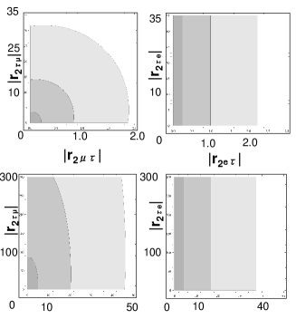
Figure 1: Upper bounds on FCNC couplings $(|r_{2X\tau}|,|r_{2\tau X}|),\quad X=e,\mu$. The top two panels obtained from the decays $\tau\to l_{X}\eta$ and the bottom two panels from $\tau\to l_{X}\pi^{0}$. The dark shaded regions correspond to $M_{A}=100$ GeV and the brightest ones correspond to $M_{A}=300$ GeV. The region in the middle of them corresponds to $M_{A}=200$ GeV. $\tan\beta$ is chosen as $14.1$.

4 Summary of constraints

We summarize the constraints on FCNC couplings.

$$|r_{2\mu\tau}|<0.9(\frac{M_{A}}{200})^{2},|r_{2e\tau}|<1(\frac{M_{A}}{200})^{2}.$$ (15)

The constraints from $\tau\to\eta$ mode are more stringent than those of $\tau\to\pi^{0}$ because the coupling of the strangeness quark with Higgs is much stronger than those of the other light quarks,

$$Br(\tau\to l_{X}\eta)\geq\frac{p_{\eta}}{24\pi\Gamma_{\tau}}\left(\frac{fm^{2}_{\pi^{+}}m_{\tau}G_{F}}{\sqrt{2}M_{A}^{2}\cos^{2}\beta}\right)^{2}$$

$$(\tan\beta(\Delta_{d}-2\Delta_{s})+\cot\beta\Delta_{u})^{2}$$

$$\{\frac{1+\delta^{2}_{l_{X}}-\delta^{2}_{\eta}}{2}(|r_{2X\tau}|^{2}+|r_{2\tau X}|^{2}\delta^{2}_{l_{X}})$$

$$-2\delta^{2}_{l_{X}}|r_{2\tau X}r_{2X\tau}|)\},$$ (16)

where $\Delta_{s}=\frac{2m_{s}}{m_{u}+m_{d}}\sim 26,\Delta_{d}\sim 1.5,\Delta_{u}\sim 0.5$ and we treat $\eta$ meson as a pure octet.

5 Possible effect on FCCC process

Using the constraint determined by FCNC processes and assuming charged Higgs boson mass , one can estimate how large FCCC can be. The hadronic invariant mass ($\sqrt{s}$) distribution for $\tau\to K^{-}\pi^{0}\nu$ decay including the FCCC effect is

$$\sum_{X=e,\mu,\tau}\frac{d{\rm Br}(\tau\to\nu_{X}K^{-}\pi^{0})}{d\sqrt{s}}=$$

$$\frac{1}{\Gamma}\frac{G_{F}^{2}|V_{us}|^{2}}{2^{5}\pi^{3}}\frac{(m_{\tau}^{2}-s)^{2}}{m_{\tau}^{3}}p_{K}$$

$$\left(\frac{m_{\tau}^{2}}{2}\Large|1-\frac{s}{M_{H}^{2}}\tan^{2}\beta(1-\frac{r_{2\tau\tau}}{\sin\beta})\Large|^{2}|F_{s}|^{2}\right.$$

$$\left.+\frac{m_{\tau}^{2}}{2}(\frac{s\tan^{2}\beta}{M_{H}^{2}\sin\beta})^{2}(|r_{2e\tau}|^{2}+|r_{2\mu\tau}|^{2})|F_{s}|^{2}\right),$$

$$\left.+(\frac{2m_{\tau}^{2}}{3s}+\frac{4}{3}){p_{K}}^{2}|F|^{2}\right),$$ (17)

where $F$ is vector form factor and $F_{s}$ is scalar form factor defined by,

$$\langle\pi^{0}K^{+}|\bar{u}\gamma_{\mu}s|0\rangle=$$

$$F(Q^{2})q_{\mu}+(F_{s}(Q^{2})-\frac{\Delta_{K\pi}}{Q^{2}}F(Q^{2}))Q_{\mu},$$ (18)

and $Q_{\mu}=p_{K}+p_{\pi},q=p_{K}-p_{\pi}$. In Fig.2, We show the FCCC contribution normalized by the standard model contribution,

$$R(\sqrt{s})=\frac{\sum_{X=e,\mu}\frac{dB_{r}(\tau\to K^{-}\pi^{0}\nu_{X})}{d\sqrt{s}}}{\frac{dB_{r}(\tau\to K^{-}\pi^{0}\nu_{\tau})}{d\sqrt{s}}{\Huge|}_{\rm S.M.}}.$$ (19)

We found the effect of FCCC is at most O$(10^{-7})\sim O(10^{-4})$ for the charged Higgs mass $M_{H}=215$(GeV) when the flavor changing couplings are chosen as $r_{e\tau}=0.9,r_{\mu\tau}=1$ and $\tan\beta$ is $14.1$.

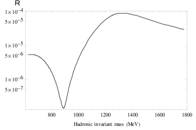
Figure 2: The FCCC contributions to the hadronic mass distribution in $\tau\to\nu_{X}K\pi$ decays ($X=e,\mu$).

6 The form factors of $\tau\to K\pi\nu$

To obtain Fig.2, the form factors for the process have been computed. Using the form factors in Eq.(18), one can compare the theoretical predictions with the experimentally measured one. They are important for study of the hadronic mass distribution and the angular distribution of $\tau\to K\pi\nu$ decay [6]. In experimental side, Belle and Babar measured the hadronic mass distribution [7, 8] for $\tau^{+}\to K_{s}\pi^{+}\overline{\nu}$ and $\tau^{-}\to K^{-}\pi^{0}\nu$ respectively. The former process is identical to $\tau^{+}\to K^{+}\pi^{0}\overline{\nu}$ in the isospin limit with CP violation of $K^{0}\overline{K^{0}}$ mixing neglected. We summarize the results related to $\tau^{\pm}\to K_{s}\pi^{\pm}\nu$ [7].

• The hadronic mass distribution and the branching fraction are measured. $Br(\tau^{-}\to K_{s}\pi^{-}\nu)=0.404\pm 0.002\pm 0.013\%$

• The experimentally measured spectrum is combined with the Breit-Wigner form of the several resonances. The fit to the spectrum leads to $K^{\ast}$ mass larger than the mass measured in hadronic processes. Belle’s result leads to $m_{K^{\ast}}=895.47\pm 0.20\pm 0.44\pm 0.59$ MeV, which is larger than $891.66\pm 0.26$ MeV. The latter value is hadronically produced $K^{\ast}$ mass average of PDG 2010.
  The width of $K^{\ast}$ is measured by the same process. The obtained value $\Gamma_{K^{\ast}}=46.2\pm 0.6\pm 1.0\pm 0.6\pm 0.7$ MeV is also different from the width measured in hadronic reactions which average is $50.8\pm 0.9$ MeV.

• Belle estimated the branching fraction for the process going through the $K^{\ast}$ resonance as, $Br(\tau^{-}\to K^{\ast-}\nu)Br(K^{\ast-}\to K^{-}\pi^{0})=(3.77\pm 0.02\pm 0.12\pm 0.12)\times 10^{-3}$. Combined it with $Br(K^{\ast-}\to K_{s}\pi^{-})=\frac{1}{3}$, PDG 2010 estimated $Br(\tau^{-}\to K^{\ast-}\nu)\sim 1.13\%$.

7 Chiral Lagrangian including vector resonance

To compute the form factors, we use the chiral Lagrangian including vector resonances. A new point of our analysis is that we compute the corrections in one loop level without spoiling the chiral counting. The rigorous one loop amplitude is identical to the one of chiral perturbation. However, in order to reproduce the effect of intermediate resonance contribution, one needs to go beyond the simple O$(p^{4})$ chiral perturbation. For the purpose, we resum the chiral corrections to vector meson self-energy. We perform the resummation so that the procedure does not spoil the O$(p^{4})$ corrections. Therefore our method is consistent with the chiral perturbation at O($p^{4}$) level. This feature is important so that our frame work reproduces the correct behaviour for the hadronic invariant mass distribution at threshold where chiral perturbation is valid. On the other hand, by resumming the self-energy corrections, one can recover the resonance behaviour even far away from the threshold region. To renormalize the one loop amplitudes, we identify the counter terms.

Denoting $V$ as SU(3)_f octet of vector mesons ($K^{\ast},\rho,...$) and $\pi$ as octet pseudoscalars ($\pi,K,\eta_{8}$), the Lagrangian including the counter terms are given as,

$${\cal L}={\cal L}^{CHPT(0)}+M_{V}^{2}{\rm Tr}(V_{\mu}-\frac{\alpha_{\mu}}{g})^{2}+{\cal L}_{c},$$ (20)

where $\alpha_{\mu}\sim\frac{1}{f^{2}}[\pi,\partial_{\mu}\pi].$ $M_{V}$ denotes the chiral limit mass for vector meson. In principle, the value can be extracted from the lattice calculation by extrapolating the vector meson mass with the finite pseudoscalar meson mass to the chiral limit, i.e., $m_{u},m_{d},m_{s}\to 0$. As for the counter terms, we note the following counter terms are needed to subtract the divergences in one loop level.

$${\cal L}_{c} = {\cal L}^{CHPT(2)}-\frac{Z_{V}}{2}{\rm Tr}F_{V\mu\nu}F_{V}^{\mu\nu}$$ (21)

$$+ C_{1}{\rm Tr}\left(\frac{\xi\chi\xi+\xi^{\dagger}\chi^{\dagger}\xi^{\dagger}}{2}\right)(V_{\mu}-\frac{\alpha_{\mu}}{g})^{2}$$

$$+ C_{2}{\rm Tr}\left(\frac{\xi\chi\xi+\xi^{\dagger}\chi^{\dagger}\xi^{\dagger}}{2}\right){\rm Tr}(V_{\mu}-\frac{\alpha_{\mu}}{g})^{2}$$

$$+ iC_{3}{\rm Tr}F_{V}^{\mu\nu}\alpha_{\perp\mu}\alpha_{\perp\nu}$$

$$+ C_{4}{\rm Tr}(\xi F_{V}^{\mu\nu}\xi^{\dagger}F_{L\mu\nu})\quad,\alpha_{\perp}\sim\frac{\partial\pi}{f},$$

where $\chi={\rm diag.}(m_{\pi}^{2},m_{\pi}^{2},2m_{K}^{2}-m_{\pi}^{2})$ and $\xi=e^{i\frac{\pi}{f}}$. $C_{1}\sim C_{4}$ and $Z_{V}$ are coefficients of the counter terms.

8 The strangeness changing charged current in terms of hadrons

In the model in Eq.(21), the strangeness changing charged current is given as,

$$\overline{u_{L}}\gamma_{\mu}s_{L}=\frac{M_{V}^{2}}{\sqrt{2}g}K_{\mu}^{\ast-}$$

$$-i\frac{K^{-}\stackrel{{\scriptstyle\leftrightarrow}}{{\partial}}\pi^{0}}{2\sqrt{2}}\left((1-\frac{M_{V}^{2}}{2g^{2}f^{2}})\sqrt{Z_{K}Z_{\pi}}\right.$$

$$\left.+\frac{2m_{K}^{2}+m_{\pi}^{2}}{f^{2}}(8L_{4}-\frac{C_{2}}{2g^{2}})\right.$$

$$+\left.\frac{2m_{K}^{2}}{f^{2}}(4L_{5}-\frac{C_{1}}{2g^{2}})\right)+\frac{4iL_{5}}{\sqrt{2}f^{2}}\Delta_{K\pi}K^{-}\partial_{\mu}\pi^{0}$$

$$+\frac{\sqrt{2}iL_{9}}{f^{2}}\partial^{\nu}(\partial_{\nu}K^{-}\partial_{\mu}\pi^{0}-\partial_{\mu}K^{-}\partial_{\nu}\pi^{0}).$$ (22)

Within tree level, including the contribution of $K^{*}$ exchange diagram, the result of the low energy theorem is reproduced as the sum of the direct $K\pi$ production process and the $K^{*}$ production process as the intermediate state,

$$<\pi^{0}K^{+}|\bar{u}\gamma_{\mu}s|0>|_{\rm dir.}=-\frac{q_{\mu}}{\sqrt{2}}(1-\frac{M_{V}^{2}}{2g^{2}f^{2}}),$$

(23)

$$<\pi^{0}K^{+}|\bar{u}\gamma_{\mu}s|0>|_{\rm K^{*}}=\frac{M_{V}^{2}q_{\mu}}{4gf^{2}}\frac{-1}{M_{V}^{2}}\frac{\sqrt{2}M_{V}^{2}}{g}.$$

The sum of them leads to,

$$F=-\frac{1}{\sqrt{2}},\quad F_{s}=\frac{\Delta_{K\pi}}{Q^{2}}F.$$ (25)

Beyond the tree level, one needs to compute four topologies of Feynman diagrams.

Figure 3: The one loop diagrams which contribute to $K\pi$ form factors. The crossed circle ($\otimes$) denotes the insertion of the charged current . The solid lines (the dotted lines) correspond to pseudoscalar(vector) meson. The vector meson propagator is $\frac{ig_{\mu\nu}}{M_{V}^{2}}$. The black blob denotes the counter term. In the top line, one loop corrections to $K\pi$ vertex are shown. In the second line, the diagrams with one loop corrections to $K^{\ast}\to K\pi$ vertex are shown. In the bottom line, the diagrams with one loop corrections to the $K^{\ast}$ production amplitude are shown.

The form factors in one-loop level correspond to the Feynman diagrams shown in Fig.3 and the self-energy diagrams shown in Fig.4. By adding the tree and one loop amplitudes, we found the result is the same as that of the one-loop chiral perturbation theory [9] except the point that one needs to replace the counter term $l_{9}$ with $l_{9\rm{eff}}$,

$$l_{9\rm{eff}}=l_{9}+\frac{c_{3}}{8g}-\frac{c_{4}}{2g}+\frac{z_{V}}{4g^{2}},$$ (26)

where $l_{9}$,$c_{3}$, $c_{4}$ and $z_{V}$ are finite parts of the coefficient of the counter terms. Then the vector form factor can be written with the function,

$$f_{+}^{CHPT}(s)=1+\frac{3}{2}(H_{K\pi}(s)+H_{K\eta}(s)),$$ (27)

$$H_{PQ}=\frac{1}{f^{2}}(sM_{PQ}(s)-L_{PQ}(s))+\frac{2}{3f^{2}}l_{9{\rm eff}}s,$$

where the functions $H,M,L$ are defined in [9].

8.1 Form Factors beyond one loop

In our framework, we can resum the self-energy diagrams of the vector meson. The resummed propagator may have the pole at complex plane which corresponds to the resonance ($\rho,K^{\ast}$).

Figure 4: The form factor contribution from the self-energy of $K^{*}$. The self-energy corrections due to $K,\pi,\eta$ mesons loop are summed as the dressed propagator.

The resummed propagator is obtained by inverting the one loop corrected inverse propagator. Denotaing $\delta A$ and $\delta B$ as chiral corrections to vector meson self energy including the counter terms of the Lagrangian $(Z_{V},C_{1},C_{2})$, the relation between the propagator and its inverse is,

$$[(M_{V}^{2}+\delta A)g^{\mu\nu}+\delta BQ^{\mu}Q^{\nu})]D_{\nu\rho}=\delta^{\mu}_{\rho}.$$ (28)

Then the resummed propagator can be easily obtained.

$$D_{\mu\nu}=\frac{1}{M_{V}^{2}+\delta A}(g_{\mu\nu}-\frac{Q_{\mu}Q_{\nu}\delta B}{M_{V}^{2}+\delta A+Q^{2}\delta B}).$$ (29)

The new contribution due to the resummed propagator to the form factor is given as:

$$\delta<\pi^{0}K^{+}|\bar{u}\gamma_{\mu}s|0>=-\frac{M_{V}^{4}}{2\sqrt{2}g^{2}f^{2}}q^{\nu}$$

$$(D_{\nu\mu}-\frac{g_{\nu\mu}}{M_{V}^{2}}+\frac{\delta Ag_{\nu\mu}+Q_{\nu}Q_{\mu}\delta B}{M_{V}^{4}}).$$ (30)

Note that we subtracted the contribution due to the bare propagator and once self-energy insertion. Then the form factors for which the resummation is taken account of are given as,

$$F_{s}=-\frac{\Delta_{K\pi}}{\sqrt{2}Q^{2}}\times$$

$$\left(f_{0}^{\rm CHPT}+\frac{(\delta A_{K}^{\ast}+Q^{2}\delta B_{K}^{\ast})^{2}}{2g^{2}f^{2}(M_{V}^{2}+\delta A_{K}^{\ast}+Q^{2}\delta B_{K}^{\ast})}\right),$$

$$F=\frac{-1}{\sqrt{2}}\left(f_{+}^{\rm CHPT}+\frac{1}{2g^{2}f^{2}}\frac{(\delta A_{K}^{\ast})^{2}}{M_{V}^{2}+\delta A_{K}^{\ast}}\right).$$ (31)

9 Comparison with the Belle Data

The prediction on hadron invariant mass spectrum using our form factors is compared with the data of $\tau\to K_{s}\pi^{-}\nu$ from [7] shown with error bars in Fig.5.

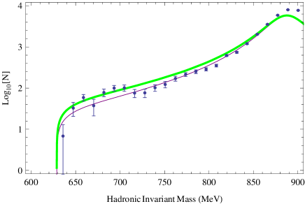
Figure 5: The hadronic invariant mass spectrum for $\tau\to K\pi\nu$ decay at low invariant mass region. The green thick solid line and the thin purple line correspond to predictions based on the theoretical model with $M_{V}=700$ and $850$ (MeV), respectively. The data is taken from [7].

At the low invariant mass region, our result is consistent with the measured spectrum. However, around the resonance region, our result is smaller than the measured spectrum. The improved treatment will be given elsewhere. A previous study with the dispersive approach is shown in [10].

10 Acknowledgement

We would like to thank Prof. George Lafferty and his colleagues for organizing the workshop. We also thank for Dr.D. Epifanov for providing us with the hadronic mass distribution. KYL is supported in part by WCU program through the KOSEF funded by the MEST (R31-2008-000-10057-0) and the Basic Science Research Program through the National Research Foundation of Korea (NRF) funded by the Korean Ministry of Education, Science and Technology (2010-0010916). TM is supported by Grant-in-Aid for Scientific Research (C) (No.22540283) from JSPS.

References

• [1] M. Sher, Phys. Rev. D66, 057301 (2002).
• [2] W. Li, Y. Yang and X. Zhang, Phys. Rev. D73, 073005 (2006).
• [3] C. H. Chen and C. Q. Geng, Phys. Rev. D74, 035010 (2006).
• [4] Y. Miyazaki et.al., Phys. Lett.B648, 341 (2007).
• [5] B. Aubert et.al., Phys. Rev. Lett. 98,061803 (2007).
• [6] D. Kimura, K. Y. Lee, T. Morozumi and
K. Nakagawa, Nucl.Phys.Proc.Suppl.189:84,
(2009), arXiv:0808.0674 (unpublished).
• [7] D. Epifanov et.al., Phys. Lett.B654, 65(2007).
• [8] B. Aubert et.al., Phys.Rev. D76,051104,
(2007).
• [9] J. Gasser and H. Leutwyler, Nucl. Phys.B250, 465(1985), Nucl. Phys.B250,517(1985).
• [10] M. Jamin, A. Pich, and J. Portoles, Phys.Lett.B664,78(2008), Phys.Lett.B640,
176(2006).