Network algorithmics and the emergence of information integration in cortical models

Abstract

An information-theoretic framework known as integrated information theory (IIT) has been introduced recently for the study of the emergence of consciousness in the brain [D. Balduzzi and G. Tononi, PLoS Comput. Biol. 4, e1000091 (2008)]. IIT purports that this phenomenon is to be equated with the generation of information by the brain surpassing the information which the brain’s constituents already generate independently of one another. IIT is not fully plausible in its modeling assumptions, nor is it testable due to severe combinatorial growth embedded in its key definitions. Here we introduce an alternative to IIT which, while inspired in similar information-theoretic principles, seeks to address some of IIT’s shortcomings to some extent. Our alternative framework uses the same network-algorithmic cortical model we introduced earlier [A. Nathan and V. C. Barbosa, Phys. Rev. E 81, 021916 (2010)] and, to allow for somewhat improved testability relative to IIT, adopts the well-known notions of information gain and total correlation applied to a set of variables representing the reachability of neurons by messages in the model’s dynamics. We argue that these two quantities relate to each other in such a way that can be used to quantify the system’s efficiency in generating information beyond that which does not depend on integration, and give computational results on our cortical model and on variants thereof that are either structurally random in the sense of an Erdős-Rényi random directed graph or structurally deterministic. We have found that our cortical model stands out with respect to the others in the sense that many of its instances are capable of integrating information more efficiently than most of those others’ instances.

I Introduction

Explaining the emergence of consciousness out of the massive neuronal interactions that take place in the brain is the greatest unsolved problem in neuroscience. It defies our ability to define what it means for the brain to be in a conscious state and, lacking a definition, also our ability to pinpoint the mechanisms that give rise to such a state and its evolution. The most recent player in the quest for a framework for consciousness studies is the integrated information theory (IIT) Balduzzi and Tononi (2008). This theory is information-theoretic in nature and seeks to characterize consciousness on the formal grounds of how information originating at different parts of the brain gets integrated as neurons interact with one another. IIT has been met with enthusiasm (cf., e.g., Koch (2009)), but substantial further developments are needed to help clarify whether this is justified.

IIT is defined on a directed graph having a node for each of a group of variables. These variables’ values evolve in lockstep (i.e., in discrete time, much as in a cellular automaton Ilachinski (2001)) in such a way that, at time $t+1$, the value of a particular variable is a function of its own value and of those of its in-neighbors in the graph at time $t$. Each node is thus assumed to have a local function that it applies on inputs to get an output per time unit. Typically a variable’s possible values are $0$ or $1$ and a node’s local function is one of the elementary logical operations. The basic tenet of IIT is that consciousness is to be equated with the surplus of information that the system is capable of generating, relative to the total information that is generated by its parts independently of one another, as it evolves from an initial state of maximum uncertainty to a final state. The use of “parts” here refers to a specific partition of the set of variables. The information surplus that IIT considers is the minimum over all possible partitions.

Unless a lot of regularity is present, computing this minimum information surplus requires a number of partitions to be examined that is given in the worst case by the Bell number corresponding to the number of variables. The Bell number for as few as $20$ variables, say, is already of the order of $10^{13}$ Sloane (2010), so the task at hand is computationally intractable even for modestly sized systems. Another potential obstacle to the success of IIT in eventually fulfilling the promise of helping characterize the emergence of consciousness is the apparent oversimplistic character of some of its elements. In our view, these include the use of binary variables and operations (even if probabilistic), and also the assumption that the system evolves in time in a synchronous and memoryless fashion.

Here we study the emergence of information integration while striving both to adhere to the spirit of IIT and to address its potential shortcomings. The main elements of our approach are the following.

(a) We adopt a cortical model with ample provisions for randomness, asynchrony, and neuronal memory. This model is the same we used previously in Nathan and Barbosa (2010), having a structural component and a functional one. The structural component is a random directed graph and attempts to portray, to the fullest possible extent, whatever structural characteristics cortices can at present be said to have. The model’s functional component, in turn, prescribes a randomized distributed algorithm to run on the graph. This algorithm uses message passing to mimic inter-neuron signaling over synapses. It is also fully asynchronous, meaning that local actions are triggered by message arrivals independently of what is happening elsewhere in the graph. At each node, the algorithm is capable of providing enough bookkeeping for some of the node’s history to be influential on current actions.

(b) We adopt two interrelated indicators of information integration. The first is simply information gain, that is, the amount of information the system generates as a single entity from an initial situation of maximum uncertainty. The second is total correlation, which in essence indicates by how much the first indicator surpasses the nodes’ total gain of information when each node’s gain is considered independently of all others’. Unlike IIT, the variables involved in our approach do not bear directly on the fire/hold dichotomy of binary local states but on whether the corresponding nodes are reached by messages as the computation unfolds.

The distributed algorithm in (a) requires at least one node to behave non-reactively at the beginning of a run. That is, at least one node must have the chance to send messages out spontaneously without any incoming message to trigger its actions. The algorithm admits any number of such initiators to act concurrently. Choosing the nodes to do it in each run is a random process. Together with the randomness already present in the graph’s structure and in the algorithm, this random choice of initiators leads to an assessment of the indicators described in (b) that takes place by averaging them over a number of graphs and/or a number of runs on each graph, each run with a new set of initiators. Vis-à-vis the treatment of information integration in IIT, which makes reference to an optimal partition of the set of variables, our approach is to generate a great number of message-flow patterns and to measure information integration as an expected, rather than optimal, quantity.

We regard the present work as being fully in line with several others that have recently attempted to draw on graph-based methods to help solve problems in neuroscience Sporns et al. (2004, 2005); Achard et al. (2006); Bassett and Bullmore (2006); He et al. (2007); Honey et al. (2007); Reijneveld et al. (2007); Sporns et al. (2007); Stam and Reijneveld (2007); Yu et al. (2008). These works are all based on highly abstract models of the underlying biological system, but some researchers believe that a complete understanding of the system’s properties can only come from considering every possible detail, even down to the molecular level. So a sort of methodological chasm is beginning to appear, as documented in the news item found in Lindley (2010). As in the present work’s predecessor Nathan and Barbosa (2010), here we adopt what might be called the artificial-life stance Forbes (2000), which essentially posits the middle alternative of employing only as much modeling detail as required to let some “life as it could be” properties emerge. Vague though this sounds, the cortical model we use has been shown to give rise to some such properties Nathan and Barbosa (2010). Specifically, by relying on the combination of its two main components (one structural, the other functional), our model gives rise, with excellent agreement, to experimentally obtained lognormal distributions of synaptic strengths Song et al. (2005). Moreover, by including enough detail of inter-neuron signaling so that the all-important local histories Barbour et al. (2007) can always be retrieved for careful examination, our model also reveals signs of the very rich dynamics that everyone agrees must underlie all cortical functions.

We proceed according to the following layout. The two components of our cortical model are reviewed in Secs. II and III. Then we move, in Sec. IV, to a description of the information-integration indicators to be used. We give computational results in Sec. V and follow these with discussion and conclusions, in Secs. VI and VII, respectively.

II Network model

The structural portion of our cortical model is the same as in Nathan and Barbosa (2010). It consists of a directed graph $D$ having $n$ nodes, one for each neuron. In $D$, an edge leading from node $i$ to node $j$ indicates that a synapse exists between the axon of the neuron that node $i$ represents and one of the dendrites of the neuron represented by node $j$. The existence of such an edge, therefore, amounts to the possibility of direct causal influence of what happens at node $i$ upon what happens at node $j$. In the same vein, indirect causal influence of what happens at node $i$ upon what happens at farther nodes can also exist, provided those nodes can be reached from $i$ through directed paths of $D$. If $i$ is part of any directed cycle in $D$, then it follows that present events at node $i$ can causally influence future events at the same node also through the indirect mediation of all other nodes in the cycle.

We regard $D$ as a originating from a random-graph model, so completing its definition requires that we specify how the out-degree of a randomly chosen node (its number of out-neighbors) is distributed, and also the probability that one of these out-neighbors is another randomly chosen node (this, indirectly, specifies the distribution of a randomly chosen node’s in-degree, its number of in-neighbors). Still following Nathan and Barbosa (2010), we assume that a randomly chosen node has out-degree $k>0$ with probability proportional to $k^{-1.8}$. The adoption of a scale-free law Newman (2005) with this particular exponent follows the work in Eguíluz et al. (2005); van den Heuvel et al. (2008), but one should mind the caveat given below. If $i$ is the randomly chosen node in question, what is left to specify is the probability that each out-neighbor of $i$ is precisely another randomly chosen node, say $j$. Taking inspiration from the work in Kaiser and Hilgetag (2004a, b), first we assume that the nodes of $D$ are placed uniformly at random on a radius-$1$ sphere. If $d_{ij}$ is the resulting Euclidean distance between $i$ and $j$, then each out-neighbor of $i$ coincides with $j$ with probability proportional to $e^{\lambda d_{ij}}$, with $\lambda<0$ a constant. This constant affects the size of $D$’s giant strongly connected component (GSCC) Dorogovtsev et al. (2001) heavily. The GSCC of $D$ is the largest subgraph of $D$ in which a directed path exists between any two nodes, that is, the largest subgraph in which all nodes have the potential of exerting direct or indirect causal influence upon all others. Similarly to what is explained in Nathan and Barbosa (2010), we choose $\lambda=-1$ so that the expected number of nodes in the GSCC is about $0.9n$. Henceforth, we limit all our information-integration investigations to within the GSCC of $D$.

The aforementioned caveat is the following. Even though the graph-theoretic modeling of cortices has made great progress Bullmore and Sporns (2009) since the earliest attempts (as represented, e.g., by Abeles (1991), where the random graphs of Erdős and Rényi Erdős and Rényi (1959) were used directly), our adoption of a scale-free structure is far from any form of consensus. This is not to say that cortices have no scale-free properties: in fact, it has been argued that they do indeed have such properties Yu et al. (2008); Freeman et al. (2009); Sporns (2011), including the so-called small-world characteristics Amaral et al. (2000), the presence of hubs (nodes with a great number of out-neighbors), and many others Freeman (2007). What is meant, instead, is that there exist results pointing in contradictory directions. The recent growth model in Freeman et al. (2009), for example, gives rise to an out-degree distribution that is not scale-free. If, on the other hand, we concede that this model is not fully justified biologically and look instead for topological characteristics derived from measurements on real cortices, what we find is not at the level of detail that we need (i.e., the level of neuronal wiring). Our sources for the $k^{-1.8}$ power law Eguíluz et al. (2005); van den Heuvel et al. (2008), for example, adopt the granularity of functional parts of the cortex. The latest available mapping Modha and Singh (2010) (in fact the most comprehensive to date), in contrast, adopts structural (rather than functional) granularity and leads to the conclusion of an exponential (rather than a power-law) distribution.

Another problem with these measurement-based characterizations is that all the reported distributions are in fact distributions of degrees, not out-degrees. That is, what counts for each node is its total number of neighbors (in- and out-neighbors combined). While in Nathan and Barbosa (2010) we ignored this and adopted the power law of Eguíluz et al. (2005); van den Heuvel et al. (2008) as the only measurement-based distribution available at the time, the more recent results in Modha and Singh (2010) lend, somewhat surprisingly, new support to our choice of this power law. In fact, we have found empirically that the degree distribution that results from our assumed out-degree distribution and distance-based deployment of directed edges can be approximated by an exponential over a significant range of degrees. This can be seen in Fig. 1, where the distribution of the combined in- and out-degrees of the nodes of $D$ is shown. In our view, this provides all the justification we can have at this point regarding our choice of the random-graph model. Further justification (or, more likely, adaptation) will depend on wiring-level measurements, whose availability, to the best of our knowledge, is still not foreseeable.

Figure 1: Distribution of a node’s number of neighbors (in- and out-neighbors combined) in our cortical model for $n=100$ (a) and $n=1\,000$ (b). Probabilities are shown for the complementary cumulative distribution; that is, given a number $k>0$ of neighbors, we show the probability that a randomly chosen node has strictly more than $k$ neighbors. Data are averages over $1\,000$ graphs for each value of $n$.

III Network algorithmics

In order to fully describe the cortical model we use in the present study, the structural properties of graph $D$ given in Sec. II need to be complemented with further, functional properties of the graph’s nodes and edges. A goal of the resulting model is to provide an algorithmic abstraction of cortical functioning that can mimic, to some extent, the buildup of potential at each neuron as its dendrites are reached by action potentials traveling down other neurons’ axons, as well as the eventual firing that this buildup entails with the accompanying action potential that travels down the neuron’s own axon. Another goal is to simulate the dynamics of synaptic strengths as they vary in the wake of neuronal firing.

We provide the necessary functional component of the model in the form of an asynchronous distributed algorithm Barbosa (1996). In general, such an algorithm assumes that the nodes of $D$ are capable of receiving messages from their in-neighbors in the graph, of performing local computation on the information that is thus received, and finally of sending messages to their out-neighbors. This processing may occur concomitantly at several of the graph’s nodes and edges and this is what gives the algorithm its distributed character. What gives it its asynchronous character, in turn, is the underlying assumption that the local computation at each node makes no reference to temporal quantities of a global nature. Such inherent locality gives asynchronous distributed algorithms a clear connection to most complex-network studies of the past decade, as evinced by the various contributions collected in Bornholdt and Schuster (2003); Newman et al. (2006); Bollobás et al. (2009). Surprisingly, though, to the best of our knowledge the interplay of structure and function, and its role in giving rise to global network properties, has seldom been explored. One notable example is the work in Stauffer and Barbosa (2006), where efficient information dissemination is shown to emerge from strictly local decisions. Another example is provided by the present study and its predecessor Nathan and Barbosa (2010).

The algorithm we use is the one introduced in Nathan and Barbosa (2010). As mentioned in Sec. I, here we assume that algorithm to be sufficiently certified for use in the cortical model we study because it is in Nathan and Barbosa (2010) shown to be capable of giving rise, among other things, to experimentally observed distributions of synaptic strengths. This algorithm, henceforth referred to simply as $A$, uses $v_{j}$ to represent the potential of node $j$ and $w_{ij}$ to represent the synaptic strength of the edge directed from node $i$ to node $j$. As customary, we refer to each $w_{ij}$ as a synaptic weight. We also assume that all nodes share the same rest and threshold potentials, denoted by $v^{0}$ and $v^{\mathrm{t}}$ (with $v^{0}<v^{\mathrm{t}}$), respectively, and that every synaptic weight lies in the interval $[0,1]$. Finally, nodes can be excitatory or inhibitory and $D$ contains no edge connecting two inhibitory nodes Abeles (1991).

Our specification of algorithm $A$ is based on the following procedure, called Fire, which gives a probabilistic rule for node $j$ to fire, that is, to send messages to its out-neighbors and reset its potential to the rest potential. Each of these messages is to be interpreted as the signaling by $j$ to one of its out-neighbors, through the corresponding synapse, that results from node $j$’s firing and the ensuing action potential. Procedure Fire uses a probability parameter, $p$.

Procedure Fire:

Fire with probability $p$:

1. Send a message to each out-neighbor of node $j$.

2. Set $v_{j}$ to $v^{0}$.

Node $j$ participates in a run of algorithm $A$ through a series of calls to procedure Fire with suitable $p$ values. In the first call in this series node $j$ may be one of the so-called initiators of the run. In this case its participation is restricted to calling Fire with $p=1$. All calls in which $j$ is not an initiator are reactive, in the sense that node $j$ only computes upon receiving a message from some in-neighbor. In this case, the call to Fire is part of a larger set of rules, as given next when node $i$ is the in-neighbor in question. In this larger set, the call to procedure Fire is preceded by an alteration to the potential $v_{j}$ and followed, possibly, by an alteration to the synaptic weight $w_{ij}$.

Algorithm $A$ (reactive mode):

1. If $i$ is excitatory, then set $v_{j}$ to $\min\{v^{\mathrm{t}},v_{j}+w_{ij}\}$.

2. If $i$ is inhibitory, then set $v_{j}$ to $\max\{v^{0},v_{j}-w_{ij}\}$.

3. Call procedure Fire with $p=(v_{j}-v^{0})/(v^{\mathrm{t}}-v^{0})$.

4. If firing did occur during the execution of Fire, then set $w_{ij}$ to $\min\{1,w_{ij}+\delta\}$.

5. If firing did not occur during the execution of Fire but the previous message received by node $j$ from any of its in-neighbors did cause $j$ to fire, then set $w_{ij}$ to $(1-\alpha)w_{ij}$.

In steps 4 and 5 of algorithm $A$, $\delta>0$ and $\alpha$ such that $0<\alpha<1$ are parameters meant to let the algorithm follow, though only to a limited extent, the principles of spike-timing-dependent plasticity Song et al. (2000); Abbott and Nelson (2000). These principles dictate, as a general rule, that the synaptic weight is to increase if firing occurs, decrease otherwise, always as a function of how close in time the relevant firings by nodes $i$ and $j$ are. Moreover, increases are to occur by a fixed amount, decreases by proportion Bi and Poo (1998, 2001); Kepecs and van Rossum (2002). As explained in Nathan and Barbosa (2010), $\delta$ and $\alpha$ must be such that $\delta\leq\alpha$.

Clearly, any nontrivial run of algorithm $A$ (i.e., one in which at least one message is sent) requires at least one node to behave as an initiator in the first of its calls to procedure Fire. Henceforth, we let $m\leq n$ be the number of nodes that do this, that is, the number of initiators in the run. It should also be clear, by steps 1 and 2 of algorithm $A$, that setting the initial value of $v_{j}$ to some number in the interval $[v^{0},v^{\mathrm{t}}]$ ensures that $v_{j}$ remains in this interval perpetually (this guarantees that the value to which probability $p$ is set in step 3 is always legitimate). Likewise, it follows from steps 4 and 5 that, if initialized to some number in the interval $[0,1]$, weight $w_{ij}$ remains constrained to lie in this interval for the whole run.

Any run of algorithm $A$ terminates eventually with probability $1$. That is, there necessarily comes a time during the run at which no more messages are sent and, from then on, no further processing occurs at the nodes. When graph $D$ is strongly connected (i.e., a directed path exists from any of its nodes to any other), then any firing during the run causes messages to be sent. Similarly, any firing by a node that is not acting as initiator is preceded by accumulating and/or depleting alterations to the node’s potential, as messages arrive, relative to the value it had initially or when the node last fired. Message traffic, therefore, provides the essential backdrop against which to conduct our study of information integration.

IV Information integration

We consider $N$ discrete random variables, denoted by $X_{1},X_{2},\ldots,X_{N}$, each taking values from the set $\{0,1\}$. All of our study on how information gets integrated in a directed graph running the distributed algorithm $A$ of Sec. III is based on attaching meaning to these variables, of which there is one for each of $N\leq n$ nodes of graph $D$, and to their distributions. We do this later in this section and also in Sec. V. First, though, we establish the two indicators of information integration that will be used.

For the sake of notational conciseness, we use $\mathbf{X}$ to denote the whole sequence $X_{1},X_{2},\ldots,X_{N}$ of variables, and likewise $\mathbf{x}\in\{0,1\}^{N}$ to denote one of the possible $2^{N}$ sequences of values $x_{1},x_{2},\ldots,x_{N}\in\{0,1\}$, each for the corresponding variable. Unambiguously, then, $\mathbf{X}=\mathbf{x}$ means that $X_{1}=x_{1},X_{2}=x_{2},\ldots,X_{N}=x_{N}$. If $P(\mathbf{x})$ is the joint probability that $\mathbf{X}=\mathbf{x}$, then we use $P_{i}(x_{i})$ to denote the marginal probability that $X_{i}=x_{i}$ for all $i\in\{1,2,\ldots,N\}$. Clearly, $P_{i}(x_{i})$ is given by the sum of $P(\mathbf{x})$ over all $2^{N-1}$ possibilities for $\mathbf{x}$ that leave the value of $X_{i}$ fixed at $x_{i}$.

Ultimately, our indicators of information integration are expressible in terms of the Shannon entropy associated with the sequence $\mathbf{X}$ of variables given the joint distribution $P$, or with each individual variable $X_{i}$ given the corresponding marginal distribution $P_{i}$. This entropy gives, in (information-theoretic) bits, a measure of how much unpredictability the distribution embodies regarding the values of the variables. We denote the joint entropy by $H(\mathbf{X})$ and each marginal entropy by $H_{i}(X_{i})$. They are given by the well-known formulae

$$H(\mathbf{X})=-\sum_{\mathbf{x}\in\{0,1\}^{N}}P(\mathbf{x})\log_{2}P(\mathbf{x})$$ (1)

and

$$H_{i}(X_{i})=-\sum_{x_{i}\in\{0,1\}}P_{i}(x_{i})\log_{2}P_{i}(x_{i}).$$ (2)

Recall that entropy is a function of the distribution and is maximized when the distribution is uniform over its domain. Thus, $0\leq H(\mathbf{X})\leq N$ and $0\leq H_{i}(X_{i})\leq 1$.

The way our indicators become expressed as combinations of entropies is through another fundamental information-theoretic notion, that of the relative entropy, or Kullback-Leibler (KL) divergence, of two distributions Weisstein (2010). Given two joint distributions $P$ and $Q$ over the same set of $N$ variables as above, the KL divergence of $P$ relative to $Q$, here denoted by $D(P,Q)$, is given by

$$D(P,Q)=\sum_{\mathbf{x}\in\{0,1\}^{N}}P(\mathbf{x})\log_{2}\frac{P(\mathbf{x})}{Q(\mathbf{x})},$$ (3)

provided $Q(\mathbf{x})>0$ whenever $P(\mathbf{x})>0$. We have $D(P,Q)=0$ if and only if $P$ and $Q$ are the same distribution. Otherwise $D(P,Q)>0$, so the KL divergence functions as a measure of how different the two distributions are [though, in general, $D(P,Q)\neq D(Q,P)$].

IV.1 Information gain

The first of our two indicators, information gain, is the KL divergence of $P$ relative to $Q$ when the latter reflects a state of maximum unpredictability regarding the values of the $N$ variables. That is, we use $Q(\mathbf{x})=1/2^{N}$ for all $\mathbf{x}\in\{0,1\}^{N}$. We denote information gain by $G(\mathbf{X})$ and it follows from Eq. (3) that

$$G(\mathbf{X})=N-H(\mathbf{X}).$$ (4)

Evidently, $0\leq G(\mathbf{X})\leq N$.

A marginal version of information gain for $X_{i}$ can also be defined by recognizing that $Q_{i}(0)=Q_{i}(1)=0.5$. Denoting this marginal information gain by $G_{i}(X_{i})$, we have $G_{i}(X_{i})=D(P_{i},Q_{i})$, whence

$$G_{i}(X_{i})=1-H_{i}(X_{i})$$ (5)

and $0\leq G_{i}(X_{i})\leq 1$.

Our use of information gain will be based on letting $N$ be the number of nodes in the graph’s GSCC, that is, one variable per node in the GSCC of graph $D$. Moreover, $P_{i}(1)$ will be the probability that node $i$ receives at least one message during a run of algorithm $A$ on $D$. Similarly, $P(\mathbf{x})$ will be the probability that every node $i$ for which $x_{i}=1$ (and no other node) receives at least one message during the run.

IV.2 Total correlation

Our second indicator uses $Q(\mathbf{x})=\prod_{i=1}^{N}P_{i}(x_{i})$ for all $\mathbf{x}\in\{0,1\}^{N}$. That is, it addresses the question of how far the variables $X_{1},X_{2},\ldots,X_{N}$ are from being independent from one another relative to $P$. Given this choice for the joint distribution $Q$, the KL divergence $D(P,Q)$ becomes what is known as the total correlation among the $N$ variables Watanabe (1960), henceforth denoted by $C(\mathbf{X})$. It follows from Eq. (3) that

$$C(\mathbf{X})=\sum_{i=1}^{N}H_{i}(X_{i})-H(\mathbf{X})$$ (6)

. Like entropy, total correlation is expressed in bits and is a function of the joint distribution $P$. It is maximized whenever $P$ assigns zero probability to all but two of the members of $\{0,1\}^{N}$: if $\mathbf{x}$ and $\mathbf{y}$ are the two exceptions, then maximization occurs if $\mathbf{x}$ and $\mathbf{y}$ are complementary value assignments to the variables (that is, for all $i$ it holds that $x_{i}=0$ if and only if $y_{i}=1$) and moreover $P(\mathbf{x})=P(\mathbf{y})=0.5$. Under these conditions, clearly $H_{i}(X_{i})=1$ for all $i$ and $H(\mathbf{X})=1$. Therefore, $0\leq C(\mathbf{X})\leq N-1$.

By Eqs. (4)–(6), we have $C(\mathbf{X})=G(\mathbf{X})-\sum_{i=1}^{N}G_{i}(X_{i})$. That is, total correlation is the amount of information gain that surpasses the total gain provided by the variables separately. Equivalently, information gain comprises total correlation and the total marginal gain $\sum_{i=1}^{N}G_{i}(X_{i})$, i.e.,

$$G(\mathbf{X})=C(\mathbf{X})+\sum_{i=1}^{N}G_{i}(X_{i}).$$ (7)

Our use of total correlation will also be based on letting $N$ be the number of nodes in the GSCC of graph $D$. Moreover, both $P_{i}(1)$ and $P(\mathbf{x})$ will have the same meanings as given above for information gain. We will also use the ratio

$$r(\mathbf{X})=\frac{C(\mathbf{X})}{G(\mathbf{X})}$$ (8)

as an indicator of how conducive graph $D$ is, under algorithm $A$, to generating information in the form of total correlation.

IV.3 Expected values

Running the distributed algorithm $A$ of Sec. III on graph $D$ from a set of initiators alters the edges’ synaptic weights and, along with them, the joint distribution $P$. As $P$ changes, so do $G(\mathbf{X})$ and $C(\mathbf{X})$ and, in interpreting the results of Sec. V, it will be useful to have $G(\mathbf{X})$ and $C(\mathbf{X})$ values against which to gauge the values that we obtain. Using the maximum values given above for each quantity is of little meaning, since they occur only at finitely many possibilities for $P$ while $P$ itself varies over a continuum of possibilities.

We then look at the expected value of either quantity as $P$ varies. To do so, we first note that specifying $P$ is equivalent to specifying $2^{N}$ numbers in the interval $[0,1]$, provided they add up to $1$. In other words, $P$ can be identified with each and every point of the standard simplex in $2^{N}$-dimensional real space. Calculating the expected value of either $G(\mathbf{X})$ or $C(\mathbf{X})$ over this simplex requires the choice of a density function and then an integration over the simplex. Given the complexity of both the distributed algorithm and the structure of $D$, it seems unlikely that a suitable density function can be derived. Moreover, even if we assume the uniform density instead, there is still the task of integrating $G(\mathbf{X})$ and $C(\mathbf{X})$ over the simplex, which to the best of our knowledge can be done analytically for $G(\mathbf{X})$, through the expected value of $H(\mathbf{X})$ (cf. Campbell (1995) and references therein), but not for $C(\mathbf{X})$.

For sufficiently large $N$, it follows from the formula in Campbell (1995) that the expected value of $H(\mathbf{X})$ over the simplex using the uniform density tends to $N-(1-\gamma)/\ln 2$, where $\gamma\approx 0.57722$ is the Euler constant Weisstein (2010). Therefore, by Eq. (4) the expected value of $G(\mathbf{X})$ tends to the constant $(1-\gamma)/\ln 2\approx 0.6$. Similarly, it follows from Eq. (6) that $0.6$ can also be taken as an approximate upper bound on the expected value of $C(\mathbf{X})$. We also know from Campbell (1995) that, under these same conditions, $H(\mathbf{X})$ is tightly clustered about the mean, and thus so is $G(\mathbf{X})$.

V Computational results

The methodology we follow in our computational experiments is entirely analogous to the one introduced in Nathan and Barbosa (2010). The central entity in this methodology is a run of algorithm $A$ of Sec. III, using $v^{0}=-15$, $v^{\mathrm{t}}=0$, $\delta=0.0002$, and $\alpha=0.04$ at all times. A run is started by $m=50$ initiators chosen uniformly at random and progresses until termination. These values of $\delta$ and $\alpha$ are the same that in Nathan and Barbosa (2010) were shown to allow the synaptic weights to become distributed as observed experimentally. As for $v^{0}$, $v^{\mathrm{t}}$, and $m$, their values only regulate the traffic of causally disconnected messages in the graph and therefore only influence how early in a sequence of runs global properties can be expected to emerge.

For a fixed graph $D$, first we decide for each of the $N$ nodes in the graph’s GSCC whether it is to be excitatory or inhibitory. This is done uniformly at random, provided no two inhibitory nodes are directly connected to each other. We use the widely accepted proportion of $20\%$ for the number of inhibitory nodes in $D$ Abeles (1991); Ananthanarayanan and Modha (2007). All runs on graph $D$ operate on this fixed set of inhibitory nodes. Then we choose initial node potentials and synaptic weights uniformly at random from the intervals $[v^{0},v^{\mathrm{t}}]$ and $[0,1]$, respectively. We group all runs on graph $D$ into sequences. The first run in a sequence starts from the initial node potentials and synaptic weights that were chosen for the graph. Each subsequent run starts from the node potentials and synaptic weights left by the previous run. We use $50\,000$ sequences for each graph $D$, each sequence comprising $10\,000$ runs. We adopt eleven observational checkpoints along the course of each sequence. The first one occurs right at the beginning of the sequence, before any run takes place, so node potentials and synaptic weights are still the ones chosen randomly. The remaining ten checkpoints occur each after $1\,000$ additional runs in the sequence.

The purpose of each checkpoint is to allow the joint distribution $P$ of the variables $X_{1},X_{2},\ldots,X_{N}$ to be estimated and, based on it, the calculation of information gain $G(\mathbf{X})$ and total correlation $C(\mathbf{X})$. Since the marginal $P_{i}(1)$ is to reflect the probability that node $i$ receives at least one message during a run, what is done at each checkpoint is to observe the message propagation patterns that take place on graph $D$ as algorithm $A$ is executed on it. We do this by resorting to $100$ side runs of the algorithm, each beginning with the choice of a new set of $m$ initiators uniformly at random and starting from the node-potential and synaptic-weight values that are current at the checkpoint. At the end of all side runs, the main sequence of runs is resumed from these same values. For $c=1,2,\ldots,11$, the joint distribution $P$ corresponding to the $c$th checkpoint can then be estimated from the overall number of side runs, which is $5\times 10^{6}$. For the purpose of averaging the resulting $G(\mathbf{X})$ and $C(\mathbf{X})$ values, multiple instances of graph $D$ are needed. This is so in order to account for structural variations and variations in the excitatory/inhibitory character of each node (in case the graphs come from sampling from a random-graph model), and for variations in the initial node potentials and synaptic weights (in all cases, including the single case in which the structure of $D$ is deterministic; cf. below).

Estimating $P$ at the $c$th checkpoint proceeds as follows. After each side run of $A$, the point $\mathbf{x}\in\{0,1\}^{N}$ such that $x_{i}=1$ if and only if node $i$ received at least one message during the run has its number of occurrences increased by $1$. Straightforward normalization yields $P(\mathbf{x})$ after all sequences have reached that checkpoint on the graph in question and the corresponding side runs have terminated. This poses a somewhat severe storage problem, since for each $D$ we execute the sequences one after the other while handling the graphs in parallel (on different processors). Therefore, the accumulators corresponding to the various members of $\{0,1\}^{N}$ that are actually observed have to be stored concomitantly for all eleven checkpoints. There is no choice but to use external (i.e., disk-based) storage in this case, which is heavily taxing with respect to how long it takes to complete everything. So the number $5\times 10^{6}$ of side runs per checkpoint per graph cannot in practice be made substantially larger. This number, after multiplied by the number of graphs in use, is also an upper bound on how many members of $\{0,1\}^{N}$ can be observed per checkpoint, so not being able to increase it means that the number of nodes $n$ cannot be too large, either. All the results we give henceforth are then for $n=100$.

We consider three different types of graph. They are referred to as type-(i)–(iii) graphs, as follows:

(i) First is the random-graph model introduced in Sec. II as the structural component of our cortical model. Generating $D$ from this random-graph model starts with placing the $n$ nodes on the surface of a radius-$1$ sphere uniformly at random and then selecting, for each node, its out-degree and its out-neighbors. The choice of $\lambda=-1$ explained in Sec. II is specific of the $n=100$ case and yields $N\approx 90$. Also, for this value of $n$ the expected in- or out-degree in $D$ is about $3.7$. Out-degrees are by construction distributed as a power law, whereas the distribution of in-degrees has been found to be similar to the Poisson distribution (i.e., concentrated near the mean) Nathan and Barbosa (2010).

(ii) Another random-graph model that we use is the generalization of the Erdős-Rényi model to the directed case Karp (1990). Given the desired expected in- or out-degree, denoted by $z$, generating $D$ places a directed edge from node $i$ to node $j\neq i$ with probability $z/(n-1)$. The resulting in- and out-degree distributions approach the Poisson distribution of mean $z$. If $z>1$, the graph’s GSCC encompasses nearly all the graph with high probability; that is, $N\approx 100$. For consistency with our cortical model, we use $z=3.7$.

(iii) At the other extreme from our cortical model are the graphs whose structure is deterministic. We use what seems to be the simplest possible structure that ensures a strongly connected $D$ with a fixed in- or out-degree equal to $\lceil 3.7\rceil=4$ for every node, the directed circulant graph Lonc et al. (2001) generated by the integers in the interval $[1,4]$. If we assume that the nodes are numbered $0$ through $n-1$, then node $i$ has four out-neighbors, nodes $i+1$ through $i+4$, where addition is modulo $n$. For $n=100$, the $20$ inhibitory nodes are necessarily equally spaced around the directed cycle that traverses the nodes in the order $0,1,\ldots,n-1,0$, lest there be a connection between two inhibitory nodes. We have $N=100$.

All our results are given for $50$ graphs of each of types (i)–(iii) and appear in Figs. 2–4, respectively. The (a) panels in these figures give the probability distributions for the number of occurrences of those members of $\{0,1\}^{N}$ that do appear in at least one side run on at least one of the $50$ graphs for each graph type at the eleventh checkpoint. After averaging over the appropriate $50$ graphs for each type, these members number $1\,733$ for type-(i) graphs, $4\,756$ for type-(ii) graphs, and $1\,033$ for type-(iii) graphs. These illustrate the point, raised above, that the need to limit the total number of side runs per graph does indeed have an impact on how capable our methodology is to probe inside the set of all $2^{N}$ value assignments to the $N$ variables. In fact, the absolute majority of assignments are never encountered. As for the others, the probability of encountering them an increasing number of times decays as a power law [less so for type-(iii) graphs].

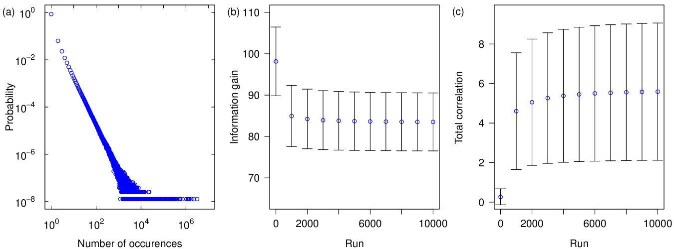
Figure 2: (Color online) Results for type-(i) graphs: (a) the probability that a randomly chosen member of $\{0,1\}^{N}$ appearing in the side runs of the last checkpoint for some graph occurs a certain number of times; (b) the average value of $G(\mathbf{X})$ at each of the checkpoints; (c) the average value of $C(\mathbf{X})$ at each of the checkpoints.

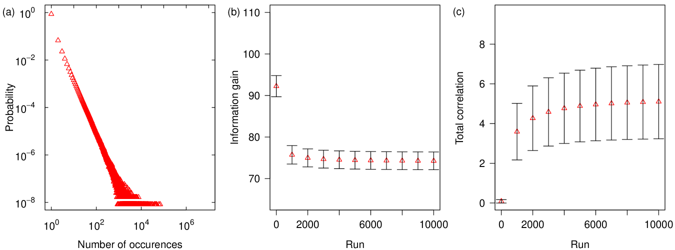
Figure 3: (Color online) Results for type-(ii) graphs: (a) the probability that a randomly chosen member of $\{0,1\}^{N}$ appearing in the side runs of the last checkpoint for some graph occurs a certain number of times; (b) the average value of $G(\mathbf{X})$ at each of the checkpoints; (c) the average value of $C(\mathbf{X})$ at each of the checkpoints.

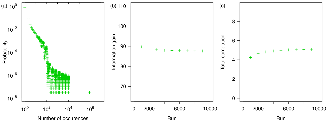
Figure 4: (Color online) Results for type-(iii) graphs: (a) the probability that a randomly chosen member of $\{0,1\}^{N}$ appearing in the side runs of the last checkpoint for some graph occurs a certain number of times; (b) the average value of $G(\mathbf{X})$ at each of the checkpoints; (c) the average value of $C(\mathbf{X})$ at each of the checkpoints.

The (b) and (c) panels in the three figures are used to show the average information gain $G(\mathbf{X})$ and total correlation $C(\mathbf{X})$, respectively, over the $50$ graphs of the corresponding graph type at each of the eleven checkpoints. Error bars are omitted from the (b) and (c) panels of Fig. 4 because the corresponding standard deviations are negligible. Because neither $G(\mathbf{X})$ nor $C(\mathbf{X})$ can surpass the number $N$ of nodes in the graph’s GSCC, and considering that not all graphs across the three graph types have the same GSCC size, all the data plotted in the (b) and (c) panels of Figs. 2–4 are normalized to this size. The latter, in turn, can be taken as $0.9n$ for type-(i) graphs and $n$ for type-(ii) and type-(iii) graphs. Our normalization procedure, therefore, has been to divide all $G(\mathbf{X})$ and $C(\mathbf{X})$ values for type-(i) graphs by $0.9$, leaving them unchanged for graphs of the other two types.

A different perspective on the results shown in Figs. 2–4 is given in Fig. 5, which presents a scatter plot of all $150$ graphs of the three types, each represented by its information gain and its total correlation at the last checkpoint. In this figure, the same normalization described above has also been used.

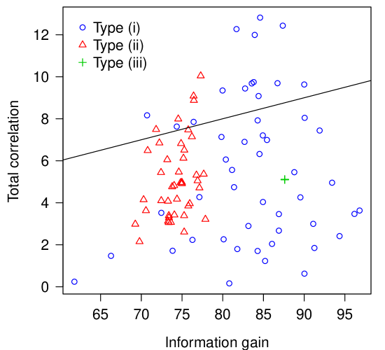
Figure 5: (Color online) A scatter plot of the $150$ different graphs used, $50$ for each of types (i)–(iii). Each graph is represented by its information gain $G(\mathbf{X})$ and its total correlation $C(\mathbf{X})$ at the last checkpoint. The straight line below which most type-(ii) and all type-(iii) graphs are found goes through the origin with slope $0.1$.

VI Discussion

The (b) panels in Figs. 2–4 demonstrate that the $G(\mathbf{X})$ averages, after a sharp decrease from the first checkpoint to the second, keep on decreasing steadily along the runs until stability is eventually reached. A similar trend is seen in the (c) panels with regard to the $C(\mathbf{X})$ averages, now with increases. (We note that reaching stability in either case is on a par with what, in Nathan and Barbosa (2010), we showed to happen with the distribution of synaptic weights under the same cortical model. That is, despite the continual modification of the weights as the dynamics goes on, their distribution reaches a steady state.) With the exception of Fig. 4, standard deviations can be significant all along the runs, particularly with regard to total correlation.

Given this variability, the plot in Fig. 5 is important and also quite revealing. First of all, it helps corroborate what the (b) and (c) panels of Figs. 2–4 already say about algorithm $A$, which essentially is what drives the system toward the eventual joint distribution $P$ over the variables $X_{1},X_{2},\ldots,X_{N}$ that is used to compute $G(\mathbf{X})$ and $C(\mathbf{X})$ for each graph. As we discussed in Sec. IV.3, should all possibilities for $P$ be equally likely, $G(\mathbf{X})$ would have a mean value of about $0.6$ over all these possibilities and would moreover be tightly clustered about this mean. The $G(\mathbf{X})$ values appearing in Fig. 5 demonstrate that algorithm $A$, independently of which graph type is used, completely subverts the uniformity hypothesis for $P$ and leads the system to generate information in amounts that surpass the $0.6$ mark very significantly. This holds also with regard to the $C(\mathbf{X})$ values in Fig. 5, whose mean under uniformly weighted $P$’s is also bounded from above by $0.6$.

Figure 5 also allows us to investigate, for each graph at the last checkpoint, how its information gain $G(\mathbf{X})$ and total correlation $C(\mathbf{X})$ are related to each other. The simplest case is that of type-(iii) graphs, whose topology and inhibitory-node positions are fixed at all times. In this case, the stochasticity of initial node potentials and synaptic weights, as well as of the functioning of algorithm $A$, are insufficient to yield any significant variation in $G(\mathbf{X})$ or $C(\mathbf{X})$ values. Next are the type-(ii) graphs, for which neither topology nor the placement of inhibitory nodes is the same for all graphs. What we see as a result is significantly more variation in $G(\mathbf{X})$ and $C(\mathbf{X})$ values, but with very few exceptions all $50$ graphs are still discernibly clustered relative to one another. Type-(i) graphs, finally, with their dependence of topology upon both a power-law-distributed out-degree and the random placement of nodes on a sphere, display $G(\mathbf{X})$ and $C(\mathbf{X})$ values that are spread over a significantly larger domain.

Aside from such broad qualitative statements, it seems hard to discriminate among the three graph types by examining either $G(\mathbf{X})$ or $C(\mathbf{X})$ values alone, even though there are type-(i) graphs for which $G(\mathbf{X})$ is greater than for any graph of the other two types, the same holding for $C(\mathbf{X})$. One simple, though effective, alternative is to resort to the ratio $r(\mathbf{X})$ defined in Eq. (8). This ratio gives the fraction of all the information generated by the system that corresponds to total correlation, that is, the fraction that corresponds to information that depends on integration among the variables. Once we adopt this metric, then the meaning of Fig. 5 becomes clearer: although all three types of graph are capable of providing significant information gain and total correlation, only type-(i) graphs (those at the basis of our cortical model) seem capable of providing an abundance of instances for which $r(\mathbf{X})$ is higher than for most type-(ii) graphs and all type-(iii) graphs.

By its very definition, the ratio $r(\mathbf{X})$ for a given graph can be regarded as an indicator of how efficient that graph is, under algorithm $A$, at integrating information. Graphs for which $r(\mathbf{X})$ is higher than for others do a better job in the sense that, of all the information that they generate, a higher fraction corresponds to information that emerges out of the integration among their constituents. What our results indicate is that type-(i) graphs, based as they are on a random-graph model, can be instantiated to specific graphs that are often more efficient than those of the other two types. The straight line drawn across Fig. 5 has slope $0.1$ and can be used as an example discriminator on the $150$ graphs represented in the figure with respect to efficiency. Specifically, all graphs above it are such that $r(\mathbf{X})>0.1$. The overwhelming majority of them are type-(i) graphs.

Justifying this behavior in terms of graph structure is still something of an open problem, though. We believe the justification has to do with the existence of hubs in type-(i) graphs, since one of their effects is to shorten distances, but whatever it is remains to be made precise. One might also think that the way in- and out-degrees get mixed in type-(i) graphs could also constitute a line of explanation, especially because these graphs have markedly different in- and out-degree distributions. If this were the case then it might be reflected in the statistical properties of these graphs’ assortativity coefficient Newman (2003), which is the Pearson correlation coefficient of the edges’ remaining out-degrees on the tail sides and remaining in-degrees on the head sides. Recall, however, that generating type-(i) graph instances, just like generating type-(ii) instances, makes no reference whatsoever to node degrees when deciding which nodes are to be joined by a given edge, so the expected assortativity coefficient of graphs of either type is zero in the limit of a formally infinite number of nodes , quite unlike the fixed structure of a type-(iii) graph (for which the assortativity coefficient is $1$). We have verified that this holds by resorting to $1\,000$ independent instances of type-(i) graphs for $n=100$ and keeping the calculations inside each graph’s GSCC. In this experiment we also found that the standard deviation of the assortativity coefficient is of the order of $10^{-2}$, so there is little variation from graph to graph.

A possible route to analyzing the role of hubs in giving rise to efficient information integration predominantly in type-(i) graphs may be to study the joint distributions of in- and out-degrees. These distributions are shown in Fig. 6, in the form of contour plots, for type-(i) and type-(ii) graphs with $n=100$. In the figure, all data are averages over the inside of each graph’s GSCC, so in- and out-degrees are expected to be no larger than $90$. While for type-(ii) graphs, in reference to part (b) of the figure, we expect no nodes to exist whose in- and out-degrees differ from each other significantly, the case of type-(i) graphs is substantially different. First of all, the data in part (a) of the figure reveal that the most common combination of in- and out-degree at a node is that in which the node has a small number of in-neighbors (between $2$ and $4$) and an even smaller number (in fact, no more than $2$) of out-neighbors. Such nodes function somewhat as type of concentrator, meaning that whenever they fire in the wake of the accumulation of signaling from its in-neighbors the resulting signal affects at most two other nodes. Hubs occur in the opposing end of this spectrum. If we take a node to be a hub when it has, say, at least $50\%$ of the other nodes as out-neighbors, then we see that, though hubs are very rare, when they occur they function as a type of disseminator: when they fire, they affect substantially more nodes than the handful of in-neighbors whose accumulated signals led to the firing itself. Perhaps it is the combination of these two types of behavior, viz. an abundance of concentrators and the occasional occurrence of a disseminator, that explains the information-integration behavior we have observed for type-(i) graphs . We expect that more research will clarify whether this is the case.

Figure 6: Contour plots of the joint distribution of a node’s in- and out-degree for type-(i) (a) and type-(ii) (b) graphs. Data are averages over $1\,000$ graphs of each type for $n=100$, always restricted to each graph’s GSCC.

VII Concluding remarks

We have introduced a network-algorithmic framework to study the emergence of information integration in directed graphs. Our original inspiration was the IIT of Balduzzi and Tononi (2008), but the resulting framework departs significantly from IIT in several aspects, most notably the adoption of the asynchronous distributed algorithm of Nathan and Barbosa (2010) to simulate neuronal processing and signaling, and the use of binary variables, one for each node in the graph’s GSCC, to signify whether nodes are reached by at least one message during a run of the algorithm. These variables have been the basis on which two information-theoretic quantities can be computed, namely information gain $G(\mathbf{X})$ and total correlation $C(\mathbf{X})$. Given the graph’s structure, the former of these indicates how much information the system generates, under the distributed algorithm, from an initial state of total uncertainty. The latter, in turn, indicates how much of this information is integrated, as opposed to the information that each node generates locally, independently of all others, denoted by $G_{i}(X_{i})$ for node $i$. For $N$ the number of variables, these quantities are related by Eq. (7). This equation, with hindsight, can nowadays be seen to have been present, at least qualitatively, in most information-theoretic views of system organization and structure (cf. Rothstein (1952) for an early example). If we stick with the basic premise of IIT, that consciousness and some form of information integration are to be equated, then what the equation says is that, of all the information that the system generates [$G(\mathbf{X})$], some reflects conscious processing [$C(\mathbf{X})$] and some unconscious processing [$\sum_{i=1}^{N}G_{i}(X_{i})$].

We have studied the behavior of information gain and total correlation for a variety of graphs. These have included (i) the random graphs that, as we know from our earlier study in Nathan and Barbosa (2010), reproduces some experimentally observed cortical properties; (ii) random graphs with Poisson-distributed in- and out-degrees; and (iii) the deterministically structured circulant graphs. While we have found that many instances of these graphs are capable of generating comparable amounts of both information gain and total correlation, those that do so efficiently (i.e., with a comparatively high $C(\mathbf{X})/G(\mathbf{X})$ ratio) are very predominantly of type (i). In the context of regarding information integration as consciousness, this seems to provide further evidence that the cortical model introduced in Nathan and Barbosa (2010) can indeed be useful as a framework for the study of cortical dynamics. Another interesting aspect, now related to the actual $G(\mathbf{X})$ and $C(\mathbf{X})$ values we have observed, is that the latter are much lower than the former. Once again, though, the association of consciousness with integrated information seems illuminating, since the overwhelming majority of all processing in the brain is believed to occur unconsciously Damasio (1999).

As it stands, our framework is only capable of handling relatively small graphs. The main difficulty is that we need to organize statistics of the frequency of occurrence of the various members of $\{0,1\}^{N}$ that appear in the runs as they elapse and this requires huge amounts of input/output operations on external storage. With current technology, the results presented in Sec. V can require up to three weeks to complete for each graph. And while the potential for parallelism is very great, normally one is also limited on the number of processors one can count on. An important direction in which to continue this research is to address these computational limitations. Success here will immediately facilitate important further research on crucial aspects of our conclusions, for example those related to how our finds scale with increasing system size. We also find our underlying cortical model, with its structural and algorithmic components, to be suitable for the undertaking of investigations on entirely different fronts. One possibility of interest to us is how to look for, and characterize, the emergence of certain oscillatory patterns of cortical activity Canolty et al. (2010). It seems that the central issue is how to reconcile such oscillations with the inherently asynchronous character of our model. This, however, remains open to further research.