Bounds on the maximum multiplicity
of some common geometric graphs

Abstract

We obtain new lower and upper bounds for the maximum multiplicity of some weighted and, respectively, non-weighted common geometric graphs drawn on $n$ points in the plane in general position (with no three points collinear): perfect matchings, spanning trees, spanning cycles (tours), and triangulations.

(i) We present a new lower bound construction for the maximum number of triangulations a set of $n$ points in general position can have. In particular, we show that a generalized double chain formed by two almost convex chains admits $\Omega(8.65^{n})$ different triangulations. This improves the bound $\Omega(8.48^{n})$ achieved by the previous best construction, the double zig-zag chain studied by Aichholzer et al.

(ii) We obtain a new lower bound of $\Omega(12.00^{n})$ for the number of non-crossing spanning trees of the double chain composed of two convex chains. The previous bound, $\Omega(10.42^{n})$, stood unchanged for more than 10 years.

(iii) Using a recent upper bound of $30^{n}$ for the number of triangulations, due to Sharir and Sheffer, we show that $n$ points in the plane in general position admit at most $O(68.62^{n})$ non-crossing spanning cycles.

(iv) We derive lower bounds for the number of maximum and minimum weighted geometric graphs (matchings, spanning trees, and tours). We show that the number of shortest tours can be exponential in $n$ for points in general position. These tours are automatically non-crossing. Likewise, we show that the number of longest non-crossing tours can be exponential in $n$. It was known that the number of shortest non-crossing perfect matchings can be exponential in $n$, and here we show that the number of longest non-crossing perfect matchings can be also exponential in $n$. It was known that the number of longest non-crossing spanning trees of a point set can be exponentially large, and here we show that this can be also realized with points in convex position. For points in convex position we obtain tight bounds for the number of longest and shortest tours. We also give a combinatorial characterization of longest tours, which yields an $O(n\log n)$ time algorithm for computing them.

Keywords: Geometric graph, non-crossing property, Hamiltonian cycle, perfect matching, triangulation, spanning tree.

1 Introduction

Let $P$ be a set of $n$ points in the plane in general position, i. e., no three points lie on a common line. A geometric graph $G=(P,E)$ is a graph drawn in the plane so that the vertex set consists of the points in $P$ and the edges are drawn as straight line segments between the corresponding points in $P$. All graphs we consider in this paper are geometric graphs. We call a graph non-crossing if its edges intersect only at common endpoints.

Determining the maximum number of non-crossing geometric graphs on $n$ points in the plane is a fundamental question in combinatorial geometry. We follow common conventions (see for instance [24]) and denote by ${\tt pg}(P)$ the number of non-crossing geometric graphs that can be embedded over the planar point set $P$, and by ${\tt pg}(n)=\max_{|P|=n}{\tt pg}(P)$ the maximum number of non-crossing graphs an $n$-element point set can admit. Analogously, we introduce shorthand notation for the maximum number of triangulations, perfect matchings, spanning trees, and spanning cycles (i. e., Hamiltonian cycles); see Table 1. For example, ${\tt tr}(n)=O(f(n))$ means that any $n$-element point set can have at most $O(f(n))$ triangulations, and ${\tt tr}(n)=\Omega(g(n))$ means that there exists some $n$-element point set that admits $\Omega(g(n))$ triangulations.

Abbr.	Graph class	Lower bound	Upper bound
pg(n)	graphs	$\Omega(41.18^{n})$ [1, 15]	$O(207.84^{n})$ [16, 26]
cf(n)	cycle-free graphs	$\mathbf{\Omega(12.26^{n})}$ [new, Theorem 2]	$O(164.49^{n})$ [16, 26]
pm(n)	perfect matchings	$\Omega^{*}(3^{n})$ [15]	$O(10.07^{n})$ [24]
st(n)	spanning trees	$\mathbf{\Omega(12.00^{n})}$ [new, Theorem 2]	$O(146.37^{n})$ [16, 26]
sc(n)	spanning cycles	$\Omega(4.64^{n})$ [15]	$\mathbf{O(68.62^{n})}$ [new, Theorem 3]
tr(n)	triangulations	$\mathbf{\Omega(8.65^{n})}$ [new, Theorem 1]	$O(30^{n})$ [26]

Table 1: Classes of non-crossing geometric (straight line) graphs, current best upper and lower bounds.

In the past 30 years numerous researchers have tried to estimate these quantities. In a pivotal result, Ajtai et al. [2] showed that ${\tt pg}(n)=O(c^{n})$ for an absolute, but very large constant $c>0$. The constant $c$ has been improved several times since then. The best bound today is $c<207.84$, which follows from a combination of a result of Sharir and Sheffer [26] with a result of Hoffmann et al. [16]. Interestingly, this upper bound, as well as the currently best upper bounds for ${\tt st}(n)$, ${\tt sc}(n)$, and ${\tt cf}(n)$, are derived from an upper bound on the maximum number of triangulations, ${\tt tr}(n)$. This underlines the importance of the bound for ${\tt tr}(n)$ in this setting. For example, the best known upper bound for ${\tt st}(n)$ is the combination of ${\tt tr}(n)\leq 30^{n}$ [26] with the ratio ${\tt sc}(n)/{\tt tr}(n)=O^{*}\left(4.879^{n}\right)$ [16]; see also previous work [22, 23, 24, 25]. To our knowledge, the only upper bound derived via a different approach is that for the number of perfect matchings by Sharir and Welzl [24], ${\tt pm}(n)=O(10.07^{n})$.

So far, we recalled various upper bounds on the maximum number of geometric graphs in certain classes. In this paper we mostly conduct our offensive from the other direction, on improving the corresponding lower bounds. Lower bounds for unweighted non-crossing graph classes were obtained in [1, 8, 15]. García, Noy, and Tejel [15] were the first to recognize the power of the double chain configuration in establishing good lower bounds for the number of matchings, triangulations, spanning cycles and trees. It was widely believed for some time that the double chain gives asymptotically the highest number of triangulations, namely $\Theta^{*}(8^{n})$. This was until 2006, when Aichholzer et al. [1] showed that another configuration, the so-called double zig-zag chain, admits $\Theta^{*}(\sqrt{72}^{n})=\Omega(8.48^{n})$ triangulations. The double zig-zag chain consists of two flat copies of a zig-zag chain. A zig-zag chain is the simplest example of an almost convex polygon. Such polygons have been introduced and first studied by Hurtado and Noy [18]. In this paper we further exploit the power of almost convex polygons and establish a new lower bound ${\tt tr}(n)=\Omega(8.65^{n})$. For matchings, spanning cycles, and plane graphs the double chain still holds the current record.

Less studied are multiplicities of weighted geometric graphs. The weight of a geometric graph is the sum of its (Euclidean) edge lengths. This leads to the question: how many graphs of a certain type (e. g., matchings, spanning trees, or tours) with minimum or maximum weight can be realized on an $n$-element point set. The notation is analogous; see Table 2. Dumitrescu [9] showed that the longest and shortest matchings can have exponential multiplicity, $2^{\Omega(n)}$, for a point set in general position. Furthermore, the longest and shortest spanning trees can also have multiplicity of $2^{\Omega(n)}$. Both bounds count explicitly geometric graphs with crossings; however these minima are automatically non-crossing. The question for the maximum multiplicity for non-crossing geometric graphs remained open for most classes of geometric graphs. Since we lack any upper bounds that are better than those for the corresponding unweighted classes, the “Upper bound” column is missing from Table 2.

Abbr.	Graph class	Lower bound
${\tt pm}_{\rm min}(n)$	shortest perfect matchings	$\Omega(2^{n/4})$ [9]
${\tt pm}_{\rm max}(n)$	longest perfect matchings	$\mathbf{\Omega(2^{n/4})}$ [new, Theorem 4]
${\tt st}_{\rm min}(n)$	shortest spanning trees	$\Omega(2^{n/2})$ [9]
${\tt st}_{\rm max}(n)$	longest spanning trees	$\mathbf{\Omega(2^{n})}$ [new, Theorem 5]
${\tt sc}_{\rm min}(n)$	shortest spanning cycles	$\mathbf{\Omega(2^{n/3})}$ [new, Theorem 7]
${\tt sc}_{\rm max}(n)$	longest spanning cycles	$\mathbf{\Omega(2^{n/3})}$ [new, Theorem 6]

Table 2: Classes of weighted non-crossing geometric graphs: exponential lower bounds.

Our results.

• A new lower bound, $\Omega(8.65^{n})$, for the maximum number of triangulations a set of $n$ points can have. We first re-derive the bound given by Aichholzer et al.  [1] with a simpler analysis, which allows us to extend it to more complex point sets. Our estimate might be the best possible for the type of construction we consider.

• A new lower bound, $\Omega(12.00^{n})$, for the maximum number of non-crossing spanning trees a set of $n$ points can have. This is obtained by refining the analysis of the number of such trees on the “double chain” point configuration. The previous bound was $\Omega(10.42^{n})$. Our analysis of the construction improves also the lower bound for cycle-free non-crossing graphs due to Aichholzer et al. [1], from $\Omega(11{.}62^{n})$ to $\Omega(12{.}23^{n})$.

• A new upper bound, $O(68.62^{n})$, for the number of non-crossing spanning cycles on $n$ points in the plane. This improves the latest upper bound of $O(70.22^{n})$ that follows from a combination of the results of Buchin et al. [6] and a recent upper bound ${\tt tr}(n)\leq 30^{n}$ by Sharir and Sheffer [26].

• New bounds on the maximum multiplicity of various weighted geometric graphs on $n$ points (weighted by Euclidean length). We show that the maximum number of longest non-crossing perfect matchings, spanning trees, spanning cycles, as well as shortest tours are all exponential in $n$. We also derive tight bounds, as well as a combinatorial characterization of longest tours (with crossings allowed) over $n$ points in convex position. This yields an $O(n\log n)$ algorithm to compute a longest tour for such sets.

The main results of this paper were presented at the 28th International Symposium on Theoretical Aspects of Computer Science (STACS) in March 2011, in Dortmund, Germany. An extended abstract (without all the proofs) appeared in the corresponding conference proceedings [13]. Since then we were able to further refine the analysis in two of our main theorems. In particular, we improved the bounds in Theorems 2 and 3.

1.1 Preliminaries

Asymptotics of multinomial coefficients.

Denote by $H(q)=-q\log q-(1-q)\log(1-q)$ the binary entropy function, where $\log$ stands for the logarithm in base 2. (By convention, $0\log{0}=0$.) For a constant $0\leq\alpha\leq 1$, the following estimate can be easily derived from Stirling’s formula for the factorial:

$${n\choose{\alpha n}}=\Theta(n^{-{1/2}}2^{H(\alpha)n}),$$ (1)

We also need the following bound on the sum of binomial coefficients; see [5] for a proof and [10, 11] for an application. If $0<\alpha\leq{1\over 2}$ is a constant,

$$\sum_{k=0}^{k\leq\alpha n}{n\choose k}\leq 2^{H(\alpha)n}.$$ (2)

Define similarly the generalized entropy function of $k$ parameters $\alpha_{1},\ldots,\alpha_{k}$, satisfying

$$\sum_{i=1}^{k}\alpha_{i}=1,\ \ \alpha_{1},\ldots,\alpha_{k}\geq 0,\$$ (3)

$$H_{k}(\alpha_{1},\ldots,\alpha_{k})=-\sum_{i=1}^{k}\alpha_{i}\log{\alpha_{i}}.$$

Clearly, $H(q)=H_{2}(q,1-q)$. Recall, the multinomial coefficient

$${n\choose n_{1},n_{2},\ldots,n_{k}}=\frac{n!}{n_{1}!n_{2}!\ldots n_{k}!},$$

where $\sum_{i=1}^{k}n_{i}=n$, counts the number of distinct ways to permute a multiset of $n$ elements, $k$ of which are distinct, with $n_{i}$, $i=1,\ldots,k$, being the multiplicities of each of the $k$ distinct elements.

Assuming that $n_{i}=\alpha_{i}n$, $i=1,\ldots,k$, for constants $\alpha_{1},\ldots,\alpha_{k}$, satisfying (3), again by using Stirling’s formula for the factorial, one gets an expression analogous to (1):

$${n\choose n_{1},n_{2},\ldots,n_{k}}=\Theta(n^{-(k-1)/2})\cdot\left(\prod_{i=1}^{k}\alpha_{i}^{-\alpha_{i}}\right)^{n}=\Theta(n^{-(k-1)/2})\cdot 2^{H_{k}(\alpha_{1},\ldots,\alpha_{k})n}.$$ (4)

Notations and conventions.

For a polygonal chain $P$, let $|P|$ denote the number of vertices. If $1<c_{1}<c_{2}$ are two constants, we frequently write $\Omega^{*}(c_{2}^{n})=\Omega(c_{1}^{n})$. A geometric graph $G=(V,E)$ is called a (geometric) thrackle, if any two edges in $E$ either cross or share a common endpoint; see e. g., [21].

2 Lower bound on the maximum number of triangulations

Hurtado and Noy [18] introduced the class $P(n,k^{r})$ of almost convex polygons. A simple polygon is in this class if it has $n$ vertices, and it can be obtained from a convex $r$-gon by replacing each edge with a “flat” reflex chain having $k$ interior vertices (thus there are $r$ reflex chains altogether), such that any two vertices of the polygon can be connected by an internal diagonal unless they belong to the same reflex chain. For example, $P(n,0^{r})$ is the class of convex polygons with $n=r$ vertices. Note that, for $r\geq 3$ and $k\geq 0$, every polygon in $P(n,k^{r})$ has $n=r(k+1)$ vertices, $r$ of which are convex.

Following the notation from [18], we denote by $t(n,k^{r})$ the number of triangulations of a polygon $P(n,k^{r})$. According to [18, Theorem 3],

$$t(n,k^{r})=\Theta\left(\left(\frac{1+k/2}{2^{k}}\right)^{r}\cdot t(n,0^{n})\right)=\Theta\left(\left(\frac{k+2}{2^{k+1}}\right)^{r}\cdot 4^{r(k+1)}\right)=\Theta\left(\left((k+2)^{\frac{1}{k+1}}\cdot 2\right)^{n}\right).$$

In particular,

• for $k=1$, $t(n,1^{r})=\Theta((2\sqrt{3})^{n})=\Theta(\sqrt{12}^{n})$. This estimate was used by Aichholzer et al.  [1] to show that the double zig-zag chain has $\Omega(8.48^{n})$ triangulations.

• for $k=2$, $t(n,2^{r})=\Theta((2^{5/3})^{n})$.

• for $k=3$, $t(n,3^{r})=\Theta((5^{1/4}\cdot 2)^{n})$.

• for $k=4$, $t(n,4^{r})=\Theta((6^{1/5}\cdot 2)^{n})$.

Analogously we define the class $P^{+}(n,k^{r})$ of almost convex (polygonal) chains. An $x$-monotone polygonal chain in this class has $n=r(k+1)+1$ vertices, and it can be obtained from an $x$-monotone convex chain with $r+1$ vertices by replacing each edge with a “flat” reflex chain with $k$ interior vertices, such that any two vertices of the chain can be connected by a segment lying above the chain unless they are incident to the same reflex chain. See Fig. 1 for a small example. To further simplify notation, we denote by $P^{+}(n,k^{r})$ any polygonal chain in this class; note they are all equivalent in the sense that they have the same visibility graph. Note that the simple polygon bounded by an almost convex chain $P^{+}(n,k^{r})$ and the segment between its two extremal vertices has $\Theta^{*}(t(n,k^{r}))$ triangulations.

Figure 1: Two (flat) mutually visible copies of $P^{+}(19,2^{6})$ with opposite orientations that form $D(38,2^{12})$. Two consecutive hull vertices of $P^{+}(19,2^{6})$ with a reflex chain of two vertices in between are indicated in both the upper and the lower chain.

In establishing our new lower bound for the maximum number of triangulations, we go through the following steps: We first describe the double zig-zag chain from [1] in our framework, and re-derive the $\Omega^{*}(\sqrt{72}^{n})$ bound of [1] for the number of its triangulations. Our simpler analysis extends to some variants of the double zig-zag chain, and leads to a new lower bound on ${\tt tr}(n)=\Omega(8.65^{n})$.

Two $x$-monotone polygonal chains $L$ and $U$ are said to be mutually visible if every pair of points, $p\in L$ and $q\in U$, are visible from each other (that is, the segment $pq$ crosses neither $U$ nor $L$).

Let us call $D(n,k^{r})$ the generalized double chain of $n$ points formed by the set of vertices in two mutually visible $x$-monotone chains, each with $n/2=r(k+1)+1$ vertices, where the upper chain is a $P^{+}(n,k^{r})$ and the lower chain is a horizontally reflected copy of $P^{+}(n,k^{r})$, as in Fig. 1. Generalized double chains are a family of point configurations, containing, among others, the double chain and double zig-zag chain configurations. In particular, $D(n,1^{r})$ is the double zig-zag chain used by Aichholzer et al. [1].

Theorem 1.

The point set $D(n,3^{r})$ with $n=8r+2$ points admits $\Omega(8.65^{n})$ triangulations. Consequently, ${\tt tr}(n)=\Omega(8.65^{n})$.

Proof.

The following estimate is used in all our triangulation bounds. Consider two mutually visible flat polygonal chains, $L$ and $U$, with $m$ vertices each ($L$ is the lower chain and $U$ is the upper chain). As in the proof of [15, Theorem 4.1], the region between the two chains consists of $2m-2$ triangles, such that exactly $m-1$ triangles have an edge along $L$ and the remaining $m-1$ triangles have an edge adjacent to $U$. It follows that the number of distinct triangulations of this middle region is

$${2m-2\choose m-1}=\Theta(m^{-1/2}\cdot 4^{m}).$$ (5)

The old $\Omega(8.48^{n})$ lower bound in a new perspective.

We estimate from below the number of triangulations of $D(n,1^{r})$ as follows. Recall that $|L|=|U|=n/2=2r+1$. Include all edges of $L$ and $U$ in any of the triangulations we construct. Now construct different triangulations as follows. Independently select a subset of $\alpha_{1}r$ short edges of ${\rm conv}(U)$ and similarly, a subset of $\alpha_{1}r$ short edges of ${\rm conv}(L)$. Here $\alpha_{1}\in(0,1)$ is a constant to be chosen later. According to (1), this can be done in

$${r\choose\alpha_{1}r}=\Theta(r^{-1/2}\cdot 2^{H(\alpha_{1})r})$$

ways in each of the two chains. Include these edges in the triangulation. Observe that after adding these short edges the middle region between the (initial) chains $L$ and $U$ is sandwiched between two mutually visible shorter chains, say $L^{\prime}\subset L$ and $U^{\prime}\subset U$, where

$$|L^{\prime}|=|U^{\prime}|=2r-\alpha_{1}r=(2-\alpha_{1})r.$$ (6)

Triangulate this middle regions in all of the possible ways, as outlined in the paragraph above (5). Let $N$ denote the total number of triangulations of $D(n,1^{r})$ obtained in this way. By the above estimate, we have $t(n,1^{r})=\Theta((2\sqrt{3})^{n})$. Combining this with (5) and (6),

$$N =\Omega^{*}\left(\left[(2\sqrt{3})^{2r}2^{H(\alpha_{1})r}\right]^{2}4^{(2-\alpha_{1})r}\right)=\Omega^{*}\left(\left[2^{2r}3^{r}2^{(2-\alpha_{1})r}2^{H(\alpha_{1})r}\right]^{2}\right)=$$

$$=\Omega^{*}\left(\left[2^{2}\cdot 3\cdot 2^{(2-\alpha_{1})}2^{H(\alpha_{1})}\right]^{2r}\right)=\Omega^{*}\left(\left[2^{4-\alpha_{1}+H(\alpha_{1})}\cdot 3\right]^{n/2}\right)=\Omega^{*}\left(a^{n}\right),$$

where

$$a=\left[2^{4-\alpha_{1}+H(\alpha_{1})}\cdot 3\right]^{(1/2)}.$$

By setting $\alpha_{1}=1/3$, as in [1], this yields $a=6\sqrt{2}=8.485\ldots$, and $N=\Omega^{*}(8.485^{n})=\Omega(8.48^{n})$.

Applying a similar analysis for a generalized double chain with reflex chains of length $3$ implies Theorem 1. To simplify the presentation we describe the next step using almost convex polygonal chains with reflex chains of length $2$.

The next step: using $D(n,2^{r})$.

Notice that in this case $n=6r+2$. In the upper chain $U$, each reflex chain of two points together with the two hull vertices next to it form a convex $4$-chain, as viewed from below. In each such $4$-chain, independently, we proceed with one of the following three choices: (0) we leave it unchanged; (1) we add one edge, so that the chain length is reduced by $1$ (from $4$ to $3$); (2) we add two edges, so that the chain length is reduced by $2$ (from $4$ to $2$). We refer to these changes and corresponding length reductions as reductions of type 0, 1 and 2, respectively. For $i=0,1,2$, let $a_{i}$ count the number of distinct ways such reductions can be performed on a convex $4$-chain of $U$. See Fig. 2(left). Clearly, we have $a_{0}=1$ and $a_{1}=a_{2}=2$.

Figure 2: Left: Length reductions for the chains of $D(n,2^{r})$: two of type $1$ and two of type $2$. Right: Length reductions for $D(n,3^{r})$: three of type $1$, five of type $2$, and five of type $3$.

For $i=0,1,2$, make $\alpha_{i}r$ reductions of type $i$ in $U$, for some suitable (constant) values $\alpha_{i}$ to be determined, with

$$\sum_{i=1}^{3}\alpha_{i}=1,\ \ \alpha_{0},\alpha_{1},\alpha_{2}\geq 0,$$

According to (4), choosing one of the three reduction types for each of the $4$-chains in $U$ can be done in

$$\Theta^{*}\left(2^{H_{3}(\alpha_{0},\alpha_{1},\alpha_{2})r}\right)$$

distinct ways. Once a reduction type $i$ has been chosen for a specific $4$-chain, it can be implemented in $a_{i}$ distinct ways. It follows that the number of distinct resulting chains $U^{\prime}$ is

$$\Theta^{*}\left(2^{H_{3}(\alpha_{0},\alpha_{1},\alpha_{2})r}\right)\prod_{i=1}^{2}a_{i}^{\alpha_{i}r}=\Theta^{*}\left(2^{H_{3}(\alpha_{0},\alpha_{1},\alpha_{2})r}\cdot 2^{\alpha_{1}r}\cdot 2^{\alpha_{2}r}\right).$$

So there are that many distinct chains $U^{\prime}$ which will occur. Proceed similarly for the lower chain $L$. Observe that once the $\alpha_{i}$ are fixed, the two resulting sub-chains $U^{\prime}\subset U$ and $L^{\prime}\subset L$ have the same length

$$|L^{\prime}|=|U^{\prime}|=3r-\alpha_{1}r-2\alpha_{2}r=(3-\alpha_{1}-2\alpha_{2})r.$$ (7)

Triangulate the middle part (between $U^{\prime}$ and $L^{\prime}$) in any of the possible ways, according to (5). Let $N$ denote the total number of triangulations obtained in this way. Recall the estimate $t(n,2^{r})=\Theta((2^{5/3})^{n})$, which yields $t(3r,2^{r})=\Theta((2^{5/3})^{3r})=\Theta(2^{5r})$. By (5) and (7), we obtain

$$N =\Omega^{*}\left(\left[(2^{5r})^{2}\cdot 2^{2H_{3}(\alpha_{0},\alpha_{1},\alpha_{2})r}\cdot 2^{2\alpha_{1}r}\cdot 2^{2\alpha_{2}r}\cdot 4^{(3-\alpha_{1}-2\alpha_{2})r}\right]\right)$$

$$=\Omega^{*}\left(\left[2^{5}\cdot 2^{H_{3}(\alpha_{0},\alpha_{1},\alpha_{2})}\cdot 2^{\alpha_{1}}\cdot 2^{\alpha_{2}}\cdot 2^{(3-\alpha_{1}-2\alpha_{2})}\right]^{2r}\right)=\Omega^{*}\left(a^{n}\right),$$

where

$$a=\left[2^{8-\alpha_{2}+H_{3}(\alpha_{0},\alpha_{1},\alpha_{2})}\right]^{1/3}.$$

The values $\alpha_{0}=\alpha_{1}=0.4$ and $\alpha_{2}=0.2$ yield $a=8.617\ldots$, and $N=\Omega^{*}(8.617^{n})=\Omega(8.61^{n})$.

The new $\Omega(8.65^{n})$ lower bound: using $D(n,3^{r})$.

We only briefly outline the differences from the previous calculation. We have $n=|D(n,3^{r})|=8r+2$. For $i=0,1,2,3$, let $a_{i}$ count the number of distinct ways reductions can be performed on a convex $5$-chain of $U$. As illustrated in Fig. 2(right), we have $a_{0}=1$, $a_{0}=3$, and $a_{2}=a_{3}=5$. The analogue of (7) is

$$|L^{\prime}|=|U^{\prime}|=4r-\alpha_{1}r-2\alpha_{2}r-3\alpha_{3}r=(4-\alpha_{1}-2\alpha_{2}-3\alpha_{3})r.$$

The estimate $t(n,3^{r})=\Theta((5^{1/4}\cdot 2)^{n})$ now yields $t(4r,3^{r})=\Theta((5^{1/4}\cdot 2)^{4r})=\Theta(5^{r}\cdot 2^{4r})$. The resulting lower bound is

$$N =\Omega^{*}\left(\left[5\cdot 2^{4}\cdot 2^{H_{4}(\alpha_{0},\alpha_{1},\alpha_{2},\alpha_{3})}\cdot 3^{\alpha_{1}}\cdot 5^{\alpha_{2}}\cdot 5^{\alpha_{3}}\cdot 2^{(4-\alpha_{1}-2\alpha_{2}-3\alpha_{3})}\right]^{2r}\right)$$

$$=\Omega^{*}\left(\left[5\cdot 2^{8-\alpha_{1}-2\alpha_{2}-3\alpha_{3}+H_{4}(\alpha_{0},\alpha_{1},\alpha_{2},\alpha_{3})}\cdot 3^{\alpha_{1}}\cdot 5^{\alpha_{2}}\cdot 5^{\alpha_{3}}\right]^{n/4}\right)=\Omega^{*}\left(a^{n}\right),$$

where

$$a=\left[5\cdot 2^{8-\alpha_{1}-2\alpha_{2}-3\alpha_{3}+H_{4}(\alpha_{0},\alpha_{1},\alpha_{2},\alpha_{3})}\cdot 3^{\alpha_{1}}\cdot 5^{\alpha_{2}}\cdot 5^{\alpha_{3}}\right]^{1/4}.$$

The values $\alpha_{0}=0.23$, $\alpha_{1}=0.34$, $\alpha_{2}=0.29$, $\alpha_{3}=0.14$, yield $a=8.6504\ldots$, and $N=\Omega^{*}(8.6504^{n})=\Omega(8.65^{n})$. The proof of Theorem 1 is now complete. ∎

Remark.

The next step in this approach, using $D(n,4^{r})$, where $n=10r+2$, seems to bring no further improvement in the bound. Omitting the details, it gives (with the obvious extended notation):

$$N \geq\Omega^{*}\left(\left[6\cdot 2^{10-\alpha_{1}-2\alpha_{2}-3\alpha_{3}-4\alpha_{4}+H_{5}(\alpha_{0},\alpha_{1},\alpha_{2},\alpha_{3},\alpha_{4})}\cdot 4^{\alpha_{1}}\cdot 9^{\alpha_{2}}\cdot 14^{\alpha_{3}}\cdot 14^{\alpha_{4}}\right]^{n/5}\right)=\Omega^{*}\left(a^{n}\right),$$

where

$$a=\left[6\cdot 2^{10-\alpha_{1}-2\alpha_{2}-3\alpha_{3}-4\alpha_{4}+H_{5}(\alpha_{0},\alpha_{1},\alpha_{2},\alpha_{3},\alpha_{4})}\cdot 4^{\alpha_{1}}\cdot 9^{\alpha_{2}}\cdot 14^{\alpha_{3}}\cdot 14^{\alpha_{4}}\right]^{1/5}.$$

Numerical experiments suggest that the maximum value of $a$ is smaller than $8.65$, with the corresponding $\alpha$-tuple near $\alpha_{0}=0.127$, $\alpha_{1}=0.254$, $\alpha_{2}=0.286$, $\alpha_{3}=0.222$, $\alpha_{4}=0.111$, which only yields $a=8.6485\ldots$. Similarly, when taking reflex chains one unit longer (using $D(n,4^{r})$, where $n=12r+2$), numerical experiments suggest that the maximum value of $a$ is smaller than $8.64$.

3 Lower bound on the maximum number of non-crossing spanning trees and forests

In this section we derive a new lower bound for the number of non-crossing spanning trees on the double-chain $D(n,0^{r})$, hence also for the maximum number of non-crossing spanning trees an $n$-element planar point set can have. The previous best bound, $\Omega(10.42^{n})$, is due to Dumitrescu [9]. By refining the analysis of [9] we obtain a new bound $\Omega(12.00^{n})$.

Theorem 2.

For the double chain $D(n,0^{r})$, we have

$$\Omega(12.00^{n})<{\tt st}(D(n,0^{r})) <O(24.68^{n}),\text{ and}$$

$$\Omega(12.26^{n})<{\tt cf}(D(n,0^{r})) <O(24.68^{n}).$$

Consequently, ${\tt st}(n)=\Omega(12.00^{n})$ and ${\tt cf}(n)=\Omega(12.26^{n}).$

Proof.

Similarly to [9], instead of spanning trees, we count (spanning) forests formed by two trees. One of the trees is associated with the lower chain $L$ and is called lower tree, while the other tree is associated with the upper chain $U$ and is called upper tree. Since the two trees can be connected in at most $O(n^{2})$ ways, it suffices to bound from below the number of forests of two such trees.

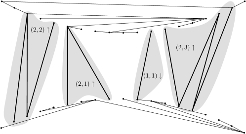
Figure 3: A double chain with lower and upper tree and four bridges.

Fig. 3 shows an example. We count only special kinds of forests: no edge of the lower tree connects two vertices of the upper chain, and similarly, no edge of the upper tree connects two vertices of the lower chain. We call the connected components of the edges between $U$ and $L$ bridges. For the class of forests we consider, bridges are subtrees of the lower or the upper tree. A bridge is called an $(i,j)$-bridge if it has $i$ vertices in $L$ and $j$ vertices in $U$. Every bridge is part of either the upper or the lower tree. In the first case we say that the bridge is oriented upwards and in the latter case that it is oriented downwards. Since edges cannot cross, the bridges have a natural left-to-right order. Fig. 3 shows four bridges, where the first bridge is an upward oriented $(2,2)$-bridge. We consider only bridges $(i,j)$, with $1\leq i,j\leq z$, for some fixed positive integer $z$. For $z=1$, our analysis coincides with the one in [9], and we first re-derive the lower bound of $\Omega(10.42^{n})$ given there. Successive improvements are achieved by considering lager values of $z$.

Let $m=n/2$ be the number of points in each chain. The distribution of bridges is specified by a set of parameters $\alpha_{ij}$, to be determined later, where the number of $(i,j)$-bridges is $\alpha_{ij}m$. To simplify further expressions we introduce the following wildcard notation:

$$\alpha_{i*}=\sum_{k=1}^{z}\alpha_{ik},\quad\alpha_{*j}=\sum_{k=1}^{z}\alpha_{kj},\quad\text{and}\quad\alpha_{**}=\sum_{k=1}^{z}\alpha_{*k}=\sum_{k=1}^{z}\alpha_{k*}.$$

A vertex is called a bridge vertex, if it is part of some bridge, and it is a tree vertex otherwise. We denote by $\alpha_{L}m$ the number of bridge vertices along $L$, and by $\alpha_{U}m$ the number of bridge vertices along $U$, we have

$$\alpha_{L}=\sum_{k=1}^{z}k\alpha_{k*},\quad\text{and}\quad\alpha_{U}=\sum_{k=1}^{z}k\alpha_{*k}.$$

To count the forests we proceed as follows. We first count the distributions of the vertices that belong to bridges on the lower ($N_{L}$) and upper chain ($N_{U}$). We then count the number of different ways in which the bridges can be realized ($N_{\text{bridges}}$) and the number of ways in which the bridges can be connected to the two trees ($N_{\text{links}}$). Finally, we estimate the number of the trees within the two chains ($N_{\text{trees}}$). All these numbers are parameterized by the variables $\alpha_{ij}$.

Consider the feasible locations of bridge vertices at the lower chain. We have ${m\choose\alpha_{L}m}$ ways to choose the bridge vertices that are in $L$. Every bridge vertex belongs to some $(i,j)$-bridge. The vertices of the bridges cannot interleave, thus we can describe the configuration of bridges by a sequence of $(i,j)$ tuples that denotes the appearance of the $\alpha_{**}m$ bridges from left to right on $L$. There are ${\alpha_{**}m\choose\alpha_{11}m,\alpha_{12}m,\dotsc,\alpha_{zz}m}$ such sequences. This give us a total of

$$N_{L}:={m\choose\alpha_{L}m}{\alpha_{**}m\choose\alpha_{11}m,\alpha_{12}m,\dotsc,\alpha_{zz}m}=\Theta^{*}\left(2^{H(\alpha_{L})m+\alpha_{**}H_{\left(z^{2}\right)}(\alpha_{11}/\alpha_{**},\dotsc,\alpha_{zz}/\alpha_{**})m}\right)$$

such “configurations” of bridge vertices along $L$.

We now determine how many options we have to place the bridge vertices on $U$. Since we have already specified the sequence of the $(i,j)$-bridges at the lower chain, all we can do is to select the bridge vertices in $U$. This gives

$$N_{U}:={m\choose\alpha_{U}m}=\Theta^{*}\left(2^{H(\alpha_{U})m}\right)$$

possibilities for the configuration on $U$.

We now study in how many ways the bridges can be added to the two trees. Since all bridges are subtrees, we can link one of the bridge vertices with the lower or upper tree. From this perspective the whole bridge acts like a super-node in one of the trees. The orientation of each bridge determines the tree it belongs to: upwards bridges to the upper tree, and downwards bridges to the lower tree. For every pair $(i,j)$ we orient half of the $(i,j)$-bridges upwards and half of them downwards. To glue the bridges to the trees we have to specify a vertex that will be linked to one of the trees. Depending on the orientation of the $(i,j)$-bridge, we have $i$ candidates for a downwards oriented bridge and $j$ candidates for an upward oriented bridge. In total we have

$$N_{\text{links}}:=\prod_{i,j}\binom{\alpha_{i,j}m}{\alpha_{i,j}m/2}\left(i^{\alpha_{ij}/2}j^{\alpha_{ij}/2}\right)^{m}=\prod_{i,j}\Theta^{*}\left(2^{\alpha_{i,j}m}\right)\left(ij\right)^{\alpha_{ij}m/2}=\Theta^{*}\left(2^{\alpha_{**}m}\right)\prod_{i,j}\left(ij\right)^{\alpha_{ij}m/2}$$

ways to link the bridges with the trees.

Until now we have specified which vertices belong to which type of bridges, the orientation of the bridges, and the vertex where the bridge will be linked to its tree. It remains to count the number of ways to actually “draw” the bridges. Let us consider an $(i,j)$-bridge. All of its edges have to go from $L$ to $U$ and the bridge has to be a tree. The number of such trees equals the number of triangulations of a polygon with point set $\{(k,0)\;|\;0\leq k\leq i\}\cup\{(k,1)\;|\;0\leq k\leq j\}$. By deleting the edges along the horizontal lines $y=0$ and $y=1$, we define a bijection between these triangulations and the combinatorial types of $(i,j)$-bridges. The number of triangulations is now easy to express similarly to Equation (5): We have $i+j-2$ triangles, and each triangle is adjacent to a horizontal edge along either $y=0$ or $y=1$, where exactly $i-1$ triangles are adjacent to line $y=0$. In total we have $B_{ij}:={i+j-2\choose i-1}$ different triangulations and therefore we can express the number of different bridges by

$$N_{\text{bridges}}=\Big{(}\prod_{ij}B_{ij}^{\alpha_{ij}}\Big{)}^{m}.$$

Figure 4: All $B_{34}=10$ combinatorial types of $(3,4)$-bridges. If an edge differs from its predecessor at the top we write a 0, otherwise a 1. We obtain a bijection between the bridges and sequences with three 1s and two 0s.

Observe that the upper and the lower trees are trees on a convex point set. By considering the bridges as super-nodes, we treat the lower chain as a convex chain of $n_{L}$ vertices. Similarly, we think of the upper chain as a convex chain with $n_{U}$ vertices. We have

$$n_{U}=\Big{(}1-\sum_{k=1}^{n}\frac{2k-1}{2}\alpha_{k*}\Big{)}m,\qquad\text{and}\qquad n_{L}=\Big{(}1-\sum_{k=1}^{n}\frac{2k-1}{2}\alpha_{*k}\Big{)}m.$$

(Notice that the bridges take away all of its vertices, except one, depending on the orientation.) Since the number of non-crossing spanning trees on an $n$-element convex point set equals $\Theta^{*}((27/4)^{n})$ [14], the number of spanning trees within the two chains is given by

$$N_{\text{trees}}=O^{*}\Big{(}\Big{(}27/4\Big{)}^{n_{L}+n_{U}}\Big{)}.$$

To finish our analysis we have to find the optimal parameters $\alpha_{ij}$ such that

$${\tt st}(D(n,0^{r}))=\Omega^{*}\left(N_{L}\cdot N_{U}\cdot N_{\text{bridges}}\cdot N_{\text{links}}\cdot N_{\text{trees}}\right)$$ (8)

is maximized.

Assume that we picked all $\alpha_{ij}$ values, except one $\alpha_{uv}$, and let $g_{uv}(\cdot)$ be the bound of (8) in terms of this only unspecified parameter. It can be observed that $g_{uv}\equiv g_{vu}$. Hence we can replace all occurrences of $\alpha_{uv}$ in (8) with $u>v$ by $\alpha_{vu}$. To solve the optimization problem we restrict ourselves to a few small values of $z$. Let us start with the case $z=1$. Here our analysis coincides with the one in [9]. We have only one parameter $\alpha_{11}$, which maximizes (8) at $4/(4+3\sqrt{6})=0.35\ldots$ and yields a lower bound of $\Omega(10.42^{n})$. A first improvement is achieved by considering $z=2$. In this case (8) is bounded by $\Omega(11.61^{n})$, which is attained at $\alpha_{11}=0{.}18,\alpha_{12}=0{.}055$, $\alpha_{22}=0{.}032$. For the next step $z=3$, we obtain a lower bound of $\Omega(11.89^{n})$, attained at $\alpha_{11}=0{.}15$, $\alpha_{12}=0{.}043$, $\alpha_{13}=0{.}010$, $\alpha_{22}=0{.}023$, $\alpha_{23}=0{.}0085$, and $\alpha_{33}=0{.}0040$. The optimal solution for $z=4$ are listed in Table 3. The induced bound equals $\Omega(12.00^{n})$. By further increasing $z$ we get improved bounds. The best bound was computed for $z=8$, namely $\Omega(12.0026^{n})$. The parameters realizing this bound can be found in Table 4. For larger $z$ we were not able to complete the numeric computations and got stuck at a local maximum, whose induced bound was smaller than $\Omega(12.0026^{n})$. All optimization problems were solved with computer algebra software.

$\alpha_{ij}$	$j=1$	$j=2$	$j=3$	$j=4$
$i\!=\!1$	$0.149$	$0.0403$	$0.00945$	$0.00208$
$i\!=\!2$	-	$0.0218$	$0.00767$	$0.00226$
$i\!=\!3$	-	-	$0.00359$	$0.00132$
$i\!=\!4$	-	-	-	$0.00058$

$\alpha_{ij}$	$j=1$	$j=2$	$j=3$	$j=4$
$i\!=\!1$	$0.151$	$0.0382$	$0.00835$	$0.00172$
$i\!=\!2$	-	$0.0192$	$0.00632$	$0.00226$
$i\!=\!3$	-	-	$0.00276$	$0.00094$
$i\!=\!4$	-	-	-	$0.00039$

Table 3: On the left: Parameters that attain the maximum $\Omega(12.00^{n})$ for ${\tt st}(D(n,0^{r}))$ for $z=4$. On the right: Parameters that attain the maximum $\Omega(12.26^{n})$ for ${\tt cf}(D(n,0^{r}))$ for $z=4$.

$\alpha_{ij}$	$i=1$	$i=2$	$i=3$	$i=4$	$i=5$	$i=6$	$i=7$	$i=8$
$j=1$	0.144	0.0389	0.00908	0.001994	0.000422	0.0000856	0.0000152	$1.76\cdot 10^{-6}$
$j=2$	-	0.0209	0.00733	0.00214	0.000569	0.000140	0.0000313	$5.12\cdot 10^{-6}$
$j=3$	-	-	0.00342	0.00125	0.000397	0.000113	0.0000290	$5.50\cdot 10^{-6}$
$j=4$	-	-	-	0.000548	0.000202	0.0000655	0.0000181	$3.34\cdot 10^{-6}$
$j=5$	-	-	-	-	0.0000845	0.0000298	$8.33\cdot 10^{-6}$	$1.25\cdot 10^{-6}$
$j=6$	-	-	-	-	-	0.0000107	$2.44\cdot 10^{-6}$	$5.10\cdot 10^{-7}$
$j=7$	-	-	-	-	-	-	$1.09\cdot 10^{-6}$	$1.31\cdot 10^{-7}$
$j=8$	-	-	-	-	-	-	-	$6.97\cdot 10^{-8}$

Table 4: Parameters that realize the maximum $\Omega(12.0026^{n})$ for ${\tt st}(D(n,0^{r}))$ for $z=8$.

Cycle-free graphs.

The same approach can be used to bound the number of cycle-free graphs (i. e., forests) on the double chain. To this end, we update Equation (8) by substituting the quantity $N_{\text{trees}}$ with

$$N_{\text{forests}}=\Omega^{*}\left(8.22469^{n_{L}+n_{U}}\right),$$

which is obtained from the bound for the number of forests on a convex point set [14]. Since we picked the bridges such that they introduce no cycles, all graphs considered by our scheme are cycle-free graphs. When the super-node (that represents a bridge) is a singleton in the forest of the chain, the combined forest could be constructed by different gluings of that bridge. For this reason we have to ignore the possibilities that were covered by $N_{\text{links}}$ to avoid over-counting. Thus we end up with

$${\tt cf}(D(n,0^{r}))=\Omega^{*}\left(N_{L}\cdot N_{U}\cdot N_{\text{bridges}}\cdot N_{\text{forests}}\right).$$

For $z=2$, our method yields the bound $\Omega(11.94^{n})$ attained at $\alpha_{11}=0{.}18$, $\alpha_{12}=0{.}039$, and $\alpha_{22}=0{.}021$; and for $z=3$ the bound $\Omega(12.16^{n})$ attained at $\alpha_{11}=0{.}12$, $\alpha_{12}=0{.}031$, $\alpha_{13}=0{.}0080$, $\alpha_{22}=0{.}016$, $\alpha_{23}=0{.}0061$, and $\alpha_{33}=0{.}0031$. The bound for $z=4$, namely $\Omega(12.26^{n})$, is attained at the parameters listed in Table 3. The best bound was obtained for $z=9$. In this case the parameters in Table 5 imply a bound of $\Omega(12.2618^{n})$. Numeric computations for larger numbers of $z$ gave no improvement on the bound for ${\tt cf}(D(n,0^{r}))$. The previous best lower bound by Aichholzer et al. was $\Omega(11.62^{n})$.

$\alpha_{ij}$	$i=1$	$i=2$	$i=3$	$i=4$	$i=5$	$i=6$	$i=7$	$i=8$	$i=9$
$j=1$	0.11	0.028	0.0069	0.0017	0.00042	0.00010	0.000024	$5.3\cdot 10^{-6}$	$1.2\cdot 10^{-6}$
$j=2$	-	0.014	0.0051	0.0017	0.00052	0.00015	0.000042	0.000011	$2.7\cdot 10^{-6}$
$j=3$	-	-	0.0025	0.0010	0.00038	0.00013	0.000042	0.000012	$3.4\cdot 10^{-6}$
$j=4$	-	-	-	0.00051	0.00022	0.000086	0.000030	0.000010	$3.1\cdot 10^{-6}$
$j=5$	-	-	-	-	0.00011	0.000047	0.000018	$6.5\cdot 10^{-6}$	$2.2\cdot 10^{-6}$
$j=6$	-	-	-	-	-	0.000024	$9.4\cdot 10^{-6}$	$3.7\cdot 10^{-6}$	$1.4\cdot 10^{-6}$
$j=7$	-	-	-	-	-	-	$5.6\cdot 10^{-6}$	$1.8\cdot 10^{-6}$	$7.5\cdot 10^{-7}$
$j=8$	-	-	-	-	-	-	-	$1.5\cdot 10^{-6}$	$3.9\cdot 10^{-7}$
$j=9$	-	-	-	-	-	-	-	-	$4.4\cdot 10^{-7}$

Table 5: Parameters that realize the maximum $\Omega(12.0026^{n})$ for ${\tt cf}(D(n,0^{r}))$ for $z=9$.

Notice that our analysis relies on numeric computations. We were able to compute the optimal parameters up to $z=8$ (for spanning trees) and up to $z=9$ (for cycle-free graphs). Table 6 lists the computed bounds with respect to the chosen parameter $z$. No significant improvements can be expected by solving the induced maximizations problems for larger values of $z$.

	$z=1$	$z=2$	$z=3$	$z=4$	$z=5$	$z=6$	$z=7$	$z=8$	$z=9$
${\tt st}$	10.424	11.611	11.899	12.004	11.952	11.998	12.002	12.002	-
${\tt cf}$	11.092	11.944	12.169	12.260	12.251	12.258	12.260	12.261	12.261

Table 6: Bases of the asymptotic exponential bounds for the number of spanning trees ${\tt st}$ and the number of cycle-free graphs ${\tt cf}$ for the point set $D(n,0^{r}))$ in terms of the parameter $z$.

For comparison, we compute an easy upper bound for both ${\tt st}(D(n,0^{r}))$ and ${\tt cf}(D(n,0^{r}))$. Every forest $F$ on the double chain splits into three parts: the induced subgraph on $L$ ($F_{L}$), the induced subgraph on $U$ ($F_{U}$) and the remaining part given by the bridge edges ($F_{B}$). The graphs $F_{L}$, $F_{U}$, and $F_{B}$ are non-crossing forests. Since the number of forests on $n$ points in convex position is $O(8.225^{n})$, there are $O(8.225^{n})$ different graphs $F_{L}\cup F_{U}$ (we rounded up to avoid the $O^{*}$ notation). It remains to bound the number of graphs $F_{B}$. Every graph counted in $F_{B}$ can be turned into a triangulation by deleting the “non-bridge vertices” and adding the appropriate edges on $L$ and $U$. Let $k$ be the number of bridge vertices on each chain. We have ${m\choose k}^{2}$ ways to select the bridge vertices. By Equation (5) we have $\Theta^{*}(4^{k})$ triangulations of the bridge vertices. In total we can bound the number of graphs $F_{B}$ from above by $\sum_{k=0}^{m}{m\choose k}^{2}4^{k}.$ To bound the exponential growth of this sum we find the dominating summand. Notice that ${m\choose k^{\prime}}^{2}4^{k^{\prime}}$ is maximized when ${m\choose k^{\prime}}2^{k^{\prime}}$ is maximized. Since $\sum_{k=0}^{m}{m\choose k}2^{k}=3^{m}$, we have ${m\choose k^{\prime}}2^{k^{\prime}}<3^{m}$, and so

$${m\choose k}^{2}4^{k}\leq{m\choose k^{\prime}}^{2}4^{k^{\prime}}<9^{m}=3^{n}.$$

Therefore the number of cycle-free non-crossing graphs on $D(n,0^{r})$ is bounded from above by $O(n\cdot 3^{n}\cdot 8.225^{n})=O(24.68^{n})$, which is also an upper bound for the number of non-crossing spanning trees on $D(n,0^{r})$. ∎

4 Upper bound for the number of non-crossing spanning cycles

Newborn and Moser [20] asked what is the maximum number of non-crossing spanning cycles for $n$ points in the plane, and they proved that $\Omega((10^{1/3})^{n})\leq{\tt sc}(n)\leq O(6^{n}\lfloor\frac{n}{2}\rfloor!)$. The first exponential upper bound ${\tt sc}(n)\leq 10^{13n}$, obtained by Ajtai et al. [2], has been followed by a series of improved bounds, e. g., see [6, 8, 24]; a more comprehensive history can be found in [7]. The current best lower bound ${\tt sc}(n)\geq 4.462^{n}$ is due to García et al. [15]. The previous best upper bound $O(70.22^{n})$ follows from combining the upper bound $30^{n/4}$ of Buchin et al.  [6] on the number of spanning cycles in a triangulation with a new upper bound of ${\tt tr}(n)\leq 30^{n}$ on the number of triangulations by Sharir and Sheffer [26] ($30^{5/4}=70.21\ldots$). The bound by Buchin et al. [6] cannot be improved much further, since they also present triangulations with $\Omega(2.0845^{n})$ spanning cycles. However, the approach of multiplying ${\tt tr}(n)$ with the maximum number of spanning cycles in a triangulation seems rather weak, since it potentially counts some spanning cycles many times.

Let $C$ be a spanning cycle. We say that $C$ has a support of $x$, and write ${\rm supp}(G)=x$ if $C$ is contained in $x$ triangulations of the point set.

Observe that a spanning cycle $C$ will be counted ${\rm supp}(C)$ times in the preceding bound. To overcome this inefficiency, we use the concept of pseudo-simultaneously flippable edges (ps-flippable edges, for short), introduced in [16]. A set $F$ of edges in a triangulation is ps-flippable if after deleting all edges in $F$, the bounded faces are convex and jointly tile the convex hull of the points. One can obtain a lower bound for the support of a spanning cycle $C$ in terms of the number of ps-flippable edges that are not in $C$. The following two properties of ps-flippable edges derived in [16] are relevant to us:

1. Every triangulation on $n$ points contains at least $\frac{n}{2}-2$ ps-flippable edges.

2. Let $C$ be a spanning cycle. Consider a triangulation $T$ that contains $C$, and has a set $F$ of ps-flippable edges. If $j$ or more edges of $F$ are not contained in $C$, then ${\rm supp}(C)\geq 2^{j}$.

We now use ps-flippable edges to improve the upper bound for the number of spanning cycles.

Theorem 3.

$\displaystyle{\tt sc}(n)=O\left(68.62^{n}\right).$

Proof.

Let $P$ be a set of $n$ points in the plane. Assume first that $n$ is even. The exact value of ${\tt sc}(P)$ is

$${\tt sc}(P)=\sum_{T}\sum_{C\subset T}\frac{1}{{\rm supp}(C)},$$ (9)

where the first sum is taken over all triangulations of $P$, and the second sum is taken over all spanning cycles contained in $T$.

Consider a triangulation $T$ over the point set $P$. By property (i), there is a set $F$ of $n/2-2$ ps-flippable edges in $T$. We wish to bound the number of spanning cycles that are contained in $T$ and use exactly $k$ edges from $F$. The support of any such cycle is at least $2^{|F|-k}$ by property (ii). There are $\binom{|F|}{k}<\binom{n/2}{k}$ ways to choose $k$ edges from $F$.

Since $n$ is even, every spanning cycle in $T$ is the union of two disjoint perfect matchings in $T$. Instead of spanning cycles containing exactly $k$ edges of $F$, we count the number of pairs of disjoint perfect matchings, $M_{1}$ and $M_{2}$, that jointly contain exactly $k$ edges of $F$. Assume, without loss of generality, that $M_{2}$ contains at least as many edges from $F$ as $M_{1}$. That is, $M_{1}$ contains at most $k/2$ edges from $F$, and $M_{2}$ at least $k/2$.

As observed by Buchin et al.  [6], a plane graph with $v$ vertices and $e$ edges contains at most $O((2e/v)^{v/4})$ perfect matchings. By Euler’s formula, a triangulation on $n$ points has at most $3n-6$ edges. Moreover, we know that both, $M_{1}$ and $M_{2}$, have to avoid the $|F|-k$ edges from $F$ that were not selected, thus it is safe to remove $|F|-k$ edges from the triangulation. Since

$$(3n-6)-(n/2-2-k)=5n/2+k-4\leq 5n/2+k,$$

the remaining graph has at most $5n/2+k$ edges and by the previous expression of Buchin et al. , there are $O\left((5+2k/n)^{(n/4)}\right)$ ways to choose $M_{1}$.

After choosing $M_{1}$, we know of at least $k/2$ edges of $F$ which participate in $M_{2}$ (the edges that were chosen from $F$ and do not participate in $M_{1}$). We can remove the endpoints of these edges (together with all incident edges). The resulting graph has at most $n-k$ vertices. We can also remove all remaining edges of $F$ and $M_{1}$, since they cannot be in $M_{2}$. It can be easily checked that overall we removed $n-2-k/2$ edges (recall that $|M_{1}|=n/2$, and that it can hold at most $k/2$ edges of $F$). Thus, given a matching $M_{1}$, the number of candidates for $M_{2}$ is

$$O\left(\left(\frac{2(3n-(n-k/2))}{n-k}\right)^{(n-k)/4}\right)=O\left(\left(\frac{4n+k}{n-k}\right)^{(n-k)/4}\right).$$

We conclude that the number of spanning cycles containing exactly $k$ edges of $F$ is

$$O\left(\binom{n/2}{k}\cdot(5+2k/n)^{(n/4)}\cdot\left(\frac{4n+k}{n-k}\right)^{(n-k)/4}\right).$$

When $k$ is small, i. e., $k\leq an$, for some $a\in(0,1/2)$, it is better to use the bound $30^{n/4}$ instead (which bounds the total number of spanning cycles in $T$). Substituting these bounds into (9) yields

$${\tt sc}(P)=\sum_{T}\left(\sum_{k=0}^{an}O\left(\frac{30^{(n/4)}}{2^{n/2-k}}\right)+\sum_{k=an}^{n/2}O\left(\binom{n/2}{k}\cdot\left(\frac{4n+k}{n-k}\right)^{(n-k)/4}\cdot\frac{(5+2k/n)^{(n/4)}}{2^{n/2-k}}\right)\right).$$

The maximum is attained for $a\approx 0.466908$, which implies

$${\tt sc}(P)=\sum_{T}O\left(2.28728^{n}\right)={\tt tr}(P)\cdot O\left(2.28728^{n}\right).$$

The upper bound ${\tt sc}(n)=O(68.62^{n})$ is immediate by substituting the upper bound ${\tt tr}(P)<30^{n}$ from [26] into the above expression.

Finally, the case where $n$ is odd can be handled as follows. Create a new point $p$ outside of ${\rm conv}(P)$, and put $P^{\prime}=P\cup\{p\}$. It can be shown that ${\tt sc}(P)\leq{\tt sc}(P^{\prime})$ by mapping every spanning cycle of $P$ to a distinct spanning cycle of $P^{\prime}$. Given a non-crossing cycle $C$ of $P$, $p$ can be connected to the two endpoints of some edge of $C$ without crossings [17, Lemma 2.1]. We can then apply the above analysis for $P^{\prime}$, obtaining the same asymptotic bound. ∎

5 Weighted geometric graphs

In this section we derive bounds on the maximum multiplicity of various weighted geometric graphs (weighted by Euclidean length).

5.1 Longest perfect matchings

Let $n$ be even, and consider perfect matchings on a set of $n$ points in the plane. It is easy to construct $n$-element point sets (no three of which are collinear) with an exponential number of longest perfect matchings: [9] gives constructions with $\Omega(2^{n/4})$ such matchings. Moreover, the same lower bound can be achieved with yet another restriction, convex position, imposed on the point set; see [9]. Here, we present constructions with an exponential number of maximum (longest) non-crossing perfect matchings.

Theorem 4.

For every even $n$, there exist $n$-element point sets with at least $2^{\lfloor n/4\rfloor}$ longest non-crossing perfect matchings. Consequently, ${\tt pm}_{\rm max}(n)=\Omega(2^{n/4})$.

Proof.

Assume first that $n$ is a multiple of $4$. Let $S_{4}=\{a,b,c,d\}$ be a $4$-element point set such that segment $ab$ is vertical, $cd$ lies on the orthogonal bisector of $ab$ (hence, $|ac|=|bc|$ and $|ad|=|bd|$), $|ab|=|cd|=\frac{1}{n}$ and $\min\{|ac|,|ad|\}=|ac|=|bc|=2n$. Then $S_{4}$ has two maximum matchings, $\{ac,bd\}$ and $\{ad,bc\}$, each of which has length at least $4n$. Let the $n$-element point set $P$ be the union of $n/4$ translated copies of $S_{4}$ lying in disjoint horizontal strips such that the copies of $a$ are almost collinear, all the copies of points $a$ and $b$ lie in a disk of unit diameter, and all the copies of points $c$ and $d$ lie in a disk of unit diameter; see Fig. 5.

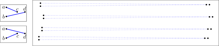
Figure 5: Left: Two possible maximum matchings for the point set $S_{4}=\{a,b,c,d\}$. Right: A set of $n=16$ points that admit $2^{4}$ maximum non-crossing perfect matchings.

If we combine the maximum matchings of all copies of $S_{4}$, then we obtain $2^{n/4}$ non-crossing perfect matchings of $P$. All these matchings have the same length, which is at least $\frac{n}{4}\cdot 4n=n^{2}$. We show that this is the maximum possible length of a non-crossing perfect matching of $P$. Let $L$ be the set of the translated copies of points $a$ and $b$; and let $R$ be the set of the translated copies of points $c$ and $d$. Then the diameter of $L$ (resp., $R$) is at most $1$, by construction. The length of any edge between $L$ and $R$ is at most $2n+1$, while all other edges have length at most $1$. If a matching has $k$ edges between $L$ and $R$, then its length is at most $k(2n+1)+(\frac{n}{2}-k)=2kn+\frac{n}{2}$, which is less than $n^{2}$ for $k<n/2$. Hence a maximum matching on $P$ is a bipartite graph between $L$ and $R$. To avoid crossings, every edge in such a bipartite graph must connect points in the same copy of $S_{4}$.

If $n$ is a multiple of $4$ plus $2$, the above construction is modified by adding a pair of points at distance $2n$, placed horizontally above all copies of $S_{4}$. This pair of points must be matched in any maximum non-crossing perfect matching of $P$. In both cases, $P$ admits at least $2^{\lfloor n/4\rfloor}$ longest non-crossing perfect matchings, as required. ∎

5.2 Non-crossing spanning trees

For minimum spanning trees, [9] gives constructions for $n$-element point sets that admit $\Omega(2^{n/4})$ such trees, and moreover, this lower bound can be attained with points in convex position. All these constructions give non-crossing spanning trees. For maximum spanning trees, [9] gives the following construction: start with two points, $a$ and $b$, and suitably place the remaining $n-2$ points on the perpendicular bisector of segment $ab$. While this configuration admits $\Omega(2^{n})$ maximum non-crossing spanning trees (which have maximum weight over all spanning trees), it uses (a large number of) collinear points. Next we show that an exponential bound, $\Omega(2^{n})$, can be achieved without allowing collinear points, and moreover, with points in convex position.

Theorem 5.

The vertex set of a regular convex $n$-gon admits $\Omega(2^{n})$ longest non-crossing spanning trees. Consequently, ${\tt st}_{\rm max}(n)=\Omega(2^{n})$.

Before proving the theorem we introduce some notation, which we will also use in Section 6. For a point set in convex position the span of an edge $xy$ is the smallest number of convex hull edges one has to traverse when going from $x$ to $y$ along the convex hull (in clockwise or counterclockwise direction). The weight of a tree $T$, denoted as $L(T)$, is the sum of its edge lengths.

Proof of Theorem 5.

Let $P$ be the vertex set of a regular $n$-gon inscribed in a circle of unit radius. Let $p\in P$ be an arbitrary element of $P$, and let $S_{p}$ be the star centered at $p$ (consisting of segments connecting $p$ to the other $n-1$ points). We first prove a counterpart for spanning trees (Lemma 1) of Alon et al. [3, Lemma 2.2], established for non-crossing matchings. Our argument is similar to that used in [3].

Lemma 1.

A longest non-crossing spanning tree on $P$ has weight $L(S_{p})$.

Proof.

Write $n=2k$ if $n$ is even, or $n=2k+1$ if $n$ is odd. Consider an arbitrary non-crossing spanning tree $T$ of $P$. Notice that the span of any edge is an integer between $1$ and $k$. For $i=1,\ldots,k$, let $N_{i}$ denote the number of edges of $T$ whose span is at least $i$. We need the following claim.

Claim. For every $i=1,\ldots,k$, we have $N_{i}\leq n-2i+1$.

Proof of Claim: The claim trivially holds for $N_{i}\leq 1$, so we can assume that $N_{i}\geq 2$. One can easily check (since $T$ is non-crossing) that there exist two edges $p_{1}p_{2}$ and $p_{3}p_{4}$ in $T$ (where $p_{2}$ could coincide with $p_{3}$), each of span at least $i$, with the following properties: (a) $p_{1},p_{2},p_{3},p_{4}$ appear in this (clockwise) order on the circle, and (b) no other edge of $T$ with span at least $i$ has an endpoint among the points between $p_{1}$ and $p_{2}$ or between $p_{3}$ and $p_{4}$. There are at least $i-1$ points on each of the two open circular arcs defined by $p_{1}p_{2}$ and $p_{3}p_{4}$. Hence all edges of $T$ with span at least $i$ are induced by at most $n-2(i-1)$ points. Since this set of edges forms a forest, it has no more than $n-2(i-1)-1=n-2i+1$ elements, as required. ∎

To finalize the proof of the lemma, we show that $L(T)\leq L(S_{p})$. For $i=1,\ldots,k$, let $\ell_{i}$ denote the (Euclidean) length of an edge with span $i$. Note that $\ell_{1}<\ell_{2}<\ldots<\ell_{k}$, and define $\ell_{0}=0$. Put also $N_{k+1}=0$, and observe that the number of edges of span $i$ is equal to $N_{i}-N_{i+1}$. Consider first the case $n=2k+1$. Straightforward algebraic manipulation gives

$$L(T) =\sum_{i=1}^{k}(N_{i}-N_{i+1})\ell_{i}=\sum_{i=1}^{k}N_{i}(\ell_{i}-\ell_{i-1})$$

$$\leq\sum_{i=1}^{k}(n-2i+1)(\ell_{i}-\ell_{i-1})=2\sum_{i=1}^{k}\ell_{i}=L(S_{p}).$$

Similarly, for $n=2k$ we get

$$L(T)\leq 2\sum_{i=1}^{k-1}\ell_{i}+\ell_{k}=L(S_{p}).$$

This concludes the proof of the lemma. ∎

To finalize the proof of Theorem 5, it remains to show that $P$ admits $\Omega(2^{n})$ non-crossing spanning trees of weight $L(S_{p})$. Denote the points in $P$ by $p_{1},p_{2},\ldots,p_{n}$ in clockwise order. We construct a family of non-crossing spanning trees on $P$. Start each tree with the same edge $T:=p_{1}p_{2}$. Repeatedly augment $T$ with one edge at a time, such that the clockwise arc spanned by the latest edge increases by one, either from its “left” (encode this choice by $0$), or from its “right” endpoint (encode this choice by $1$). Notice that regardless of the choice, the latest edge has always the same length. As a result, the clockwise arc spanning the new tree $T$ now includes one more point: either its right endpoint moves clockwise by one position, or its left endpoint moves counter-clockwise by one position. After $n-2$ steps, $T$ is a non-crossing spanning tree of $P$. If $n=2k+1$, the sequence of edge lengths (including the first edge, $p_{1}p_{2}$) is

$$\ell_{1},\ldots,\ell_{k-1},\ell_{k},\ell_{k-1},\ldots,\ell_{1}.$$

If $n=2k$, the sequence of edge lengths (including the first edge, $p_{1}p_{2}$) is

$$\ell_{1},\ldots,\ell_{k-1},\ell_{k},\ell_{k},\ell_{k-1},\ldots,\ell_{1}.$$

In both cases, the weight of each tree is $L(S_{p})$. All 0-1 sequences of length $n-2$ yield different trees, so there are at least $2^{n-2}$ longest non-crossing spanning trees, as required. This completes the proof of Theorem 5. ∎

5.3 Longest non-crossing tours

We show here that the maximum number of longest non-crossing spanning cycles is also exponential in $n$. In the next section we also show that the maximum number of shortest non-crossing spanning cycles on $n$ points is exponential in $n$ (Theorem 7).

Theorem 6.

Let ${\tt sc}_{\rm max}(n)$ denote the maximum number of longest non-crossing spanning cycles that an $n$-element point set can have. Then we have $\Omega(2^{n/3})\leq{\tt sc}_{\rm max}(n)\leq O(68.62^{n})$.

Proof.

Since we are counting non-crossing tours, we have ${\tt sc}_{\rm max}(n)=O(68.62^{n})$ by Theorem 3. It remains to show the lower bound. For every $k\in\mathbb{N}$, we construct a set $Q$ of $4k+1$ points that admits $2^{k}=\Omega(2^{n/4})$ longest non-crossing tours. We start by constructing an auxiliary set $P$ of $2k$ points. The auxiliary point set $P$ may contain collinear triples, however our final set $Q$ does not. Recall that two segments cross if and only if their relative interiors intersect. We construct $P=\{c_{i},x_{i}:i=1,2,\ldots,k\}$ with the following properties:

• for every $x_{i}$, the farthest point in $P$ is $c_{i}$;

• the perfect matching $M=\{c_{i}x_{i}:i=1,2,\ldots,k\}$ is non-crossing; and

• the convex hull of $P$ is ${\rm conv}(P)=(x_{1},c_{1},c_{2},\ldots,c_{k})$.

Note that property (i) implies that $M$ is the maximum matching of $P$.

For $k\in\mathbb{N}$, let $\alpha=\frac{\pi}{3k}$. We construct $P=\{c_{i},x_{i}:i=1,2,\ldots,k\}$ iteratively. During the iterative process, we maintain the properties that

$$|x_{i}c_{i}|>\max_{j<i}|x_{i}c_{j}|\hskip 28.45274pt\mbox{\rm and}\hskip 28.45274pt|x_{i+1}c_{i}|>\max_{j<i}|x_{i+1}c_{j}|.$$

Initially, let $c_{1}=(0,0)$, $x_{1}=(2,0)$, and $x_{2}=(2-\frac{1}{k},0)$. Let $\vec{\ell}_{1}$ be a ray emitted by $x_{1}$ and incident to $c_{1}$. Refer to Fig. 6. If $c_{i}$, $x_{i}$ and $x_{i+1}$ are already defined, we construct points $c_{i+1}$ and $x_{i+2}$ (in the last iteration, only $c_{i+1}$) as follows. Let $\vec{\ell}_{i+1}$ be a ray emitted by $x_{i+1}$ such that $\angle(\vec{\ell}_{i+1},\vec{\ell}_{i})=\alpha$. Compute the intersections of ray $\vec{\ell}_{i+1}$ with the circle centered at $x_{i}$ of radius $|x_{i}c_{i}|$ and the circle centered at $x_{i+1}$ of radius $|x_{i+1}c_{i}|$. Let $c_{i+1}\in\vec{\ell}_{i+1}$ be the midpoint of the segment between these two intersection points. This choice guarantees that $|x_{i+1}c_{i+1}|>|x_{i+1}c_{j}|$ and $|x_{j}c_{i+1}|<|x_{j}c_{j}|$ for all $j\leq i$. Now let $x_{i+2}\in c_{i+1}x_{i+1}$ be a point at distance at most $\frac{1}{k}$ from $x_{i+1}$ such that we have $|x_{i+2}c_{i+1}|>|x_{i+2}c_{j}|$ for all $j\leq i$. This completes the description of $P$.

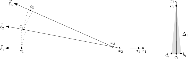
Figure 6: Left: The auxiliary point set $P$ for $k=3$. Right: A long and skinny deltoid $\Delta_{i}=(a_{i},b_{i},c_{i},d_{i})$.

Note that $|x_{i}x_{i+1}|\leq\frac{1}{k}$ for $i=1,\ldots,k-1$, and so the points $x_{1},\ldots,x_{k}$ lie in a disk of diameter $1$. Hence, for every point $x_{i}$, the farthest point in $P$ is in $\{c_{j}:j=1,\ldots,k\}$. By the above construction, the farthest point from $x_{i}$ in $\{c_{j}:j=1,\ldots,k\}$ is $c_{i}$. This proves that $P$ has property (i). It is easy to verify that $P$ has properties (ii) and (iii), as well.

We now construct the point set $Q$ based on $P$. Let $\delta>0$ be a sufficiently small constant. For every segment $c_{i}x_{i}$ we construct a skinny deltoid $\Delta_{i}=(a_{i},b_{i},c_{i},d_{i})$, see Fig. 6, such that $a_{i}\in c_{i}x_{i}$ is at distance $\delta$ from $x_{i}$, we have $|b_{i}c_{i}|=|c_{i}d_{i}|=\delta$, and $|a_{i}b_{i}|=|a_{i}c_{i}|=|a_{i}d_{i}|=|c_{i}x_{i}|-\delta$. Since the segments $c_{i}x_{i}$ are pairwise non-crossing and $\delta>0$ is small, the deltoids $\Delta_{i}$ are pairwise interior disjoint. Let $Q$ be the set of vertices of all deltoids $\Delta_{i}$, $i=1,\ldots,k$, and the point $x_{1}$. Since ${\rm conv}(P)=(c_{1},c_{2},\ldots,c_{k},x_{1})$, we have ${\rm conv}(Q)=(b_{1},c_{1},d_{1},b_{2},c_{2},d_{2},\ldots,b_{k},c_{k},d_{k},x_{1})$, and the points $\{a_{i}:i=1,\ldots,k\}$ lie in the interior of ${\rm conv}(Q)$. If $\delta>0$ is sufficiently small, then the farthest points from $a_{i}$ in $Q$ are $b_{i}$, $c_{i}$, and $d_{i}$, for every $i=1,2,\ldots,k$.

Every non-crossing tour of $Q$ visits the convex hull vertices in the cyclic order determined by ${\rm conv}(Q)$. We obtain a non-crossing tour by replacing some edges of ${\rm conv}(Q)$ with non-crossing paths visiting the points lying in the interior of ${\rm conv}(Q)$. If we replace either edge $b_{i}c_{i}$ or $c_{i}d_{i}$ with the path $(b_{i},a_{i},c_{i})$ or $(c_{i},a_{i},d_{i})$, respectively, for every $i=1,2,\ldots,k$, then we obtain a tour. Let $\mathcal{H}$ be the set of $2^{k}$ tours obtained in this way. These tours are non-crossing, since for every $i$, we exchange an edge of $\Delta_{i}$ with a path lying in $\Delta_{i}$, and the deltoids $\Delta_{i}$ are interior disjoint. The tours in $\mathcal{H}$ have the same length, $L=|{\rm conv}(Q)|-k\delta+2\sum_{i=1}^{k}|a_{i}c_{i}|$, since $|a_{i}b_{i}|=|a_{i}d_{i}|=|a_{i}c_{i}|$. It remains to show that this length is maximal. Note that a non-crossing tour cannot have an edge between two non-consecutive vertices of ${\rm conv}(Q)$. Hence, every edge that intersects the interior of ${\rm conv}(Q)$ must be incident to some point $a_{i}$ lying in the interior of ${\rm conv}(Q)$. Each $a_{i}$ is incident to two edges of a tour: The total length of these two edges is at most $2|a_{i}c_{i}|$, which is attained if $a_{i}$ is connected to $b_{i}$, $c_{i}$, or $d_{i}$. In any other case, it is less than $2|a_{i}c_{i}|-k\delta$ if $\delta>0$ is sufficiently small. The total length the edges on the boundary of the convex hull is less than $|{\rm conv}(Q)|$. So any non-crossing tour in which some point $a_{i}$ is not connected to $b_{i},c_{i}$ or to $c_{i},d_{i}$ must have length less than $L$. This implies ${\tt sc}_{\rm max}(n)=\Omega(2^{n/4})$.

To obtain the asserted bound, we use a skinny hexagon (instead of deltoid $\Delta_{i}$) with five equidistant vertices on a circle centered at $a_{i}$. We now have four possible ways to insert each $a_{i}$ into the tour, which implies ${\tt sc}_{\rm max}(n)=\Omega(4^{n/6})=\Omega(2^{n/3})$. ∎

Typically for the longest matching, spanning tree or spanning cycle, one expects to see many crossings. Somewhat surprisingly, we show that this is not always the case.

Corollary 1.

For every even $n\geq 2$, there exists an $n$-element point set (in general position) whose longest perfect matching is non-crossing.

Proof.

For every $k\geq 1$, consider the set $\{a_{i},c_{i}:i=1,2,\ldots,k\}$ of $2k$ points, and its perfect matching $\{a_{i}c_{i}:i=1,2,\ldots,k\}$ in the proof of Theorem 6. This is the longest perfect matching (over all perfect matchings of the point set, crossing or non-crossing), and moreover, it is non-crossing. ∎

6 Tours

In this section we derive estimates on the maximum multiplicity of the shortest (minimum) and, respectively, the longest (maximum) Hamiltonian tour on $n$ points (crossings allowed). While the shortest tour has the non-crossing attribute for free, the longest tour typically has crossings.

6.1 Shortest tours

Theorem 7.

Let ${\tt sc}_{\rm min}(n)$ denote the maximum number of shortest tours that an $n$-element point set can have.

• For points in convex position, there is exactly one shortest spanning cycle, i. e., ${\tt sc}_{\rm min}(n)=1$.

• For points in general position, ${\tt sc}_{\rm min}(n)$ is exponential in $n$. More precisely, $2^{\lfloor n/3\rfloor}\leq{\tt sc}_{\rm min}(n)\leq O(68.62^{n})$.

Proof.

(i) It is well known (and easy to prove) that a shortest tour of a convex point set does not admit any crossings, thus the vertices have to be visited in clockwise or counterclockwise order.

(ii) Consider now a set $S$ of $n$ points in general position. Since any minimum tour of $S$ is a non-crossing spanning cycle of $S$, by Theorem 3 we have ${\tt sc}_{\rm min}(n)\leq{\tt sc}(n)=O(68.62^{n})$.

A lower bound of $2^{\lfloor n/3\rfloor}$ is given by the following construction. Assume first that $n$ is a multiple of $3$. Consider an isosceles triangle $\Delta{abc}$ with sides $\varepsilon$, $\varepsilon$ and $\varepsilon/4$, see Fig. 7 (left).

Figure 7: Lower bound for shortest tours.

Let $S$ consist of $n/3$ rotated copies of $\Delta$ along a circle of unit radius, as in Fig. 7 (right). If $\varepsilon$ is small enough, the shortest tour of $S$ must visit the three vertices in each copy of $\Delta$ in their order along the circle. We can assume w.l.o.g. that the groups (copies) are visited in clockwise order. Then the first point visited in each group is (a rotated copy of) $a$. Since each group of three points can be minimally traversed in two ways, $a,b,c$, or $a,c,b$, the number of shortest tours is $2^{n/3}$. The construction can be easily modified for any $n$, by removing one or two points from one of the groups. ∎

6.2 Longest tours for points in convex position

In the following we give tight bounds for the number of maximum tours on $n$ points in convex position (allowing crossings) and outline how to compute such tours efficiently. The result for odd $n$ seems to have been first discovered by Ito et al. [19]. Nevertheless we present our own simpler proof here for completeness.

Theorem 8.

Let ${\tt tc}_{\rm max}(n)$ denote the maximum number of longest tours that an $n$-element point set in convex position can have. For $n$ odd we have ${\tt tc}_{\rm max}(n)=1$ and the (unique) longest tour is a thrackle. For $n$ even we have ${\tt tc}_{\rm max}(n)=n/2$.

Proof.

Let $P$ be a set of $n$ points in convex position. Assume that $n=2k$ if $n$ is even, and $n=2k-1$ if $n$ is odd. We pick an orientation for every possible tour arbitrarily. According to this orientation we denote an edge $xy$ of a tour as $x\rightarrow y$ if $x$ is the predecessor of $y$ in the tour. We call two edges $x\rightarrow y$ and $u\rightarrow v$ parallel if they are disjoint (including their endpoints) and the segments $xu$ and $yv$ are disjoint. For instance, the edges $a_{3}\rightarrow a_{2}$ and $b_{2}\rightarrow b_{3}$ in Fig. 8(b) are parallel. Two disjoint edges that are not parallel are called anti-parallel. We say two vertices of $P$ are consecutive if they define a convex hull edge. To prove the theorem we first prove three simple observations.

Observation (a): The longest tour does not contain a pair of anti-parallel edges.
Suppose the longest tour does contain anti-parallel edges $x\rightarrow y$ and $u\rightarrow v$. We delete both edges and construct a new tour by adding $x\rightarrow u$ and $y\rightarrow v$ and re-orienting the part of the old tour between $u$ and $y$. The new tour is longer since in a convex quadrilateral the sum of the diagonals exceeds the sum of two opposing side lengths.

Observation (b): In a longest tour with parallel edges $x\rightarrow y$ and $u\rightarrow v$, the vertices $x,u$ and the vertices $y,v$ are consecutive. In particular, a longest tour contains no triplet of pairwise parallel edges.
Assume that there exists a vertex $w$ “in between” $x$ and $u$ with predecessor $w^{\prime}$. Then the edge $w^{\prime}\rightarrow w$ would determine a pair of anti-parallel edges with either $x\rightarrow y$ or $u\rightarrow v$, in contradiction to Observation (a). By a similar argument one can show that $y$ and $v$ have to be consecutive.

Observation (c): The span of every edge in a longest tour is at least $k-1$.
Suppose, to the contrary, that the longest tour contains an edge $x\rightarrow y$ with span at most $k-2$. By the pigeonhole principle there is at least one edge $u\rightarrow v$ that does not cross $x\rightarrow y$. Due to Observation (b), $uv$ has to be an edge of span at least $n-k$. Let $\{L,R\}$ be the partition of $P\setminus\{x,y\}$ induced by $x\rightarrow y$ (that is, points left and right relative to $x\rightarrow y$). Assume further that $|R|>|L|$, that is, $\{u,v\}\subseteq R$. By Observation (b), a longest tour cannot contain three pairwise parallel edges. Hence, in the longest tour the points in $R\setminus\{u\}$ have to have a successor from $L\cup\{x\}$. But, again due to the pigeonhole principle, this is impossible, since $|R|-1\geq k-1$, but $|L|+1\leq k-2$.

We now proceed with the proof of Theorem 8. Assume first that $n=2k-1$ is odd. Due to observation (c), the longest tour does not have any edge of span at most $k-2$, hence the span of every edge is $k-1$, which is the largest possible span for $n$ odd. This determines the longest geometric tour. For every vertex we have only two possible edges with span $k-1$, hence the longest tour is unique.

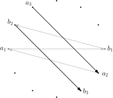
(a)		(b)

Figure 8: (a) A configuration that does not allow an extension to a longest tour, since the possible 5 “outgoing” edges have only 4 candidates to connect with. (b) A valid extension. The edges $a_{i+1}\rightarrow a_{i}$ and $b_{i}\rightarrow b_{i+1}$ form a pair of parallel edges.

Now assume that $n=2k$ is even. Notice that we have to use at least one edge of span $k$, since otherwise (using edges with span $k-1$ only) there would be two anti-parallel edges. Assume that a longest tour contains the edge $a_{1}\rightarrow b_{1}$ of span $k$. Let $a_{2}$ denote the predecessor of $a_{1}$, and $b_{2}$ denote the successor of $b_{1}$ in the longest tour. The edges $a_{2}\rightarrow a_{1}$ and $b_{1}\rightarrow b_{2}$ need to have span $k-1$. There are two possibilities for the relative position of $a_{2}a_{1}$ and $b_{2}b_{1}$. In case they cross, all outgoing edges from the vertices on the arc between $a_{1}$ and $b_{1}$ (in cyclic order of $P$, opposite from $a_{2}$ and $b_{2}$) have to cross $b_{1}\rightarrow b_{2}$. This yields a contradiction by the pigeonhole principle (see Fig. 8(a)). Thus we can assume that $a_{2}$ and $b_{2}$ are located on opposite sides of $a_{1}\rightarrow b_{1}$, as in Fig. 8(b). We extend the partial tour step by step, choosing new edges $a_{i+1}\rightarrow a_{i}$, $b_{i}\rightarrow b_{i+1}$ with span $k-1$ appropriately. If we would use an edge with span $k$ we would “close” the spanning cycle before all vertices have been visited. We stop after we found $n-1$ edges and add the final edge $b_{n/2}\rightarrow a_{n/2}$ with span $k$. To see that this scheme works correctly, notice that the edges added in every step form a pair of parallel edges with span $k-1$, which “rotates” around $P$. The construction can be characterized by the location of the edges with span $k$. Since $a_{1}$ and $b_{n/2}$ are consecutive, as well as $a_{n/2}$ and $b_{1}$, we have at most $n/2$ choices to select these two edges.

If $P$ is the vertex set of a regular $n$-gon, then $P$ has $n/2$ longest tours by rotational symmetry. The 5 longest tours for $n=10$ are depicted in Fig. 9. ∎

Figure 9: The 5 longest tours on the vertex set of a regular 10-gon. The two edges with span $5$ are drawn with bold lines.

As an immediate algorithmic corollary of Theorem 8, the longest tours on a set of $n$ points in convex position can be computed in $O(n\log{n})$ time. If $n$ is odd and the convex polygon $P=p_{0},p_{1},\ldots,p_{n-1}$ is given, the tour can be computed in $O(n)$ time: start with $i=0$, and iteratively set $i\leftarrow i+\frac{n-1}{2}$, where the indices are taken modulo $n$. If $n$ is even, we have $n/2$ candidates for the longest tour. Given a candidate, we can construct the next candidate by exchanging only 4 edges of the tour. Thus, after computing the weight of the first candidate, all other candidates can be evaluated in $O(1)$ per tour. As in the case of odd $n$, we can compute the longest tours in $O(n)$ time if the cyclic order of $P$ is given, and in $O(n\log n)$ time otherwise.

7 Conclusion

Our investigations leave some questions open:

1. We used a special point configuration, $D(n,3^{r})$, to prove a new lower bound on ${\tt tr}(n)$, the maximum number of triangulations. The question arises if this (or a similar) configuration could also give better lower bounds for other quantities we studied, such as ${\tt cf}(n)$, ${\tt st}(n)$, or ${\tt sc}(n)$. However, no analysis for other geometric graph classes has been done so far, not even for the simpler-to-analyze double zig-zag chain $D(n,1^{r})$,.

2. While for the maximum number of triangulations, the upper and lower bounds are reasonably close, this is not the case for non-crossing spanning cycles. Recall that the current best lower bound, offered by the double chain configuration is $\Omega(4.462^{n})$, and our new upper bound is only $O(68.62^{n})$. Most likely, the lower bound is closer to the truth, however the arguments are missing to justify this belief. Clearly a large gap remains to be covered.

3. Is it possible to obtain upper bounds for the maximum multiplicity of weighted configurations, better than those for the corresponding unweighted structures? For example, is ${\tt sc}_{\rm max}(n)$ significantly smaller than ${\tt sc}(n)$, or ${\tt pm}_{\rm min}(n)$ significantly smaller than ${\tt pm}(n)$?

4. For points in convex position, we devised an $O(n\log n)$-time algorithm for computing the longest tour. However, for points in general position it is not known whether this problem is NP-hard. Barvinok et al. [4] showed that the problem is solvable in $O(n)$ time under the $L_{1}$ metric [4]. On the negative side, they also show that the problem is NP-complete under the $L_{2}$ metric for points in 3-space. Nothing is known about the complexity of computing the longest non-crossing spanning tour, spanning path, perfect matching or spanning tree. However, constant ratio approximations are available for the last three problems; see [3, 12].

References

- [1] O. Aichholzer, T. Hackl, B. Vogtenhuber, C. Huemer, F. Hurtado and H. Krasser, On the number of plane geometric graphs, Graphs and Combinatorics 23(1) (2007), 67–84.
- [2] M. Ajtai, V. Chvátal, M. Newborn and E. Szemerédi, Crossing-free subgraphs, Annals Discrete Math. 12 (1982), 9–12.
- [3] N. Alon, S. Rajagopalan, and S. Suri, Long non-crossing configurations in the plane, Fundamenta Informaticae 22 (1995), 385–394. A preliminary version in Proc. 9th ACM Symp. on Comput. Geom., ACM Press, 1993, pp. 257–263.
- [4] A. I. Barvinok, S. P. Fekete, D. S. Johnson, A. Tamir, G. J. Woeginger, and R. Woodroofe, The geometric maximum traveling salesman problem, J. ACM 50(5) (2003), 641–664.
- [5] P. Beame, M. Saks and J. Thathachar, Time-space tradeoffs for branching programs, Proc. 39th Annual Symposium on Foundations of Computer Science, 1998, pp. 254–263.
- [6] K. Buchin, C. Knauer, K. Kriegel, A. Schulz, and R. Seidel, On the number of cycles in planar graphs, Proc. 13th Annual International Conference on Computing and Combinatorics, volume 4598 of LNCS, Springer, 2007, pp. 97–107.
- [7] E. Demaine, Simple polygonizations, http://erikdemaine.org/polygonization/ (version of November, 2010).
- [8] A. Dumitrescu, On two lower bound constructions, Proc. 11th Canadian Conf. on Computational Geometry, 1999, pp. 111–114.
- [9] A. Dumitrescu, On the maximum multiplicity of some extreme geometric configurations in the plane, Geombinatorics 12(1) (2002), 5–14.
- [10] A. Dumitrescu and R. Kaye, Matching colored points in the plane: some new results, Computational Geometry: Theory and Applications 19(1) (2001), 69–85.
- [11] A. Dumitrescu and W. Steiger, On a matching problem in the plane, Discrete Mathematics 211(1-3) (2000), 183–195.
- [12] A. Dumitrescu and Cs. D. Tóth, Long non-crossing configurations in the plane, Discrete and Computational Geometry 44(4) (2010), 727–752.
- [13] A. Dumitrescu, A. Schulz, A. Sheffer and Cs. D. Tóth, Bounds on the maximum multiplicity of some common geometric graphs, Proc. 28th International Symposium on Theoretical Aspects of Computer Science, Leibniz International Proceedings in Informatics (LIPIcs) 9, 2011, pp. 637–648.
- [14] P. Flajolet and M. Noy, Analytic combinatorics of non-crossing configurations, Discrete Mathematics 204 (1999), 203–229.
- [15] A. García, M. Noy and A. Tejel, Lower bounds on the number of crossing-free subgraphs of , Computational Geometry: Theory and Applications 16(4) (2000), 211–221.
-
[16]
M. Hoffmann, M. Sharir, A. Sheffer, Cs. D. Tóth, and E. Welzl,
Counting plane graphs: flippability and its applications,
Proc. Algorithms and Data Structure Symposium (WADS),
vol. 6844 of LNCS, Springer, 2011, pp. 524–535.
Also at
arxiv.org/abs/1012.0591 - [17] F. Hurtado, M. Kano, D. Rappaport, and Cs. D. Tóth: Encompassing colored planar straight line graphs, Computational Geometry: Theory and Applications 39 (1) (2008), 14–23.
- [18] F. Hurtado and M. Noy, Counting triangulations of almost-convex polygons, Ars Combinatoria 45 (1997), 169–179.
- [19] H. Ito, H. Uehara, and M. Yokoyama, Lengths of tours and permutations on a vertex set of a convex polygon, Discrete Applied Mathematics 115(1-3) (2001), 63–71.
- [20] M. Newborn and W. O. J. Moser, Optimal crossing-free Hamiltonian circuit drawings of , J. Combin. Theory Ser. B 29 (1980), 13–26.
- [21] J. Pach and P. K. Agarwal, Combinatorial Geometry, John Wiley, New York, 1995.
- [22] A. Razen, J. Snoeyink, and E. Welzl, Number of crossing-free geometric graphs vs. triangulations, Electronic Notes in Discrete Mathematics 31 (2008), 195–200.
- [23] F. Santos and R. Seidel, A better upper bound on the number of triangulations of a planar point set, Journal of Combinatorial Theory Ser. A 102(1) (2003), 186–193.
- [24] M. Sharir and E. Welzl, On the number of crossing-free matchings, cycles, and partitions, SIAM J. Comput. 36(3) (2006), 695–720.
- [25] M. Sharir and E. Welzl, Random triangulations of point sets, Proc. 22nd Annual ACM-SIAM Symposium on Computational Geometry, ACM Press, 2006, pp. 273–281.
- [26] M. Sharir and A. Sheffer, Counting triangulations of planar point sets, Electronic Journal of Combinatorics 18 (2011), P70.