Conditional symmetries and exact solutions
of the diffusive Lotka-Volterra system

Roman Cherniha^†,‡ and Vasyl’ Davydovych^†

^† Institute of Mathematics, Ukrainian National Academy of Sciences,
Tereshchenkivs’ka Street 3, Kyiv 01601, Ukraine
^‡ Department of Mathematics, National University ‘Kyiv Mohyla Academy’
2, Skovoroda Street, Kyiv 01601, Ukraine

Q-conditional symmetries of the classical Lotka-Volterra system in the case of one space variable are completely described and a set of such symmetries in explicit form is constructed. The relevant non-Lie ansätze to reduce the classical Lotka-Volterra systems with correctly-specified coefficients to ODE systems and examples of new exact solutions are found. A possible biological interpretation of some exact solutions is presented.

Keywords: Lotka-Volterra system, reaction-diffusion system, Lie symmetry, $Q$-conditional symmetry, non-classical symmetry, exact solution.

1.Introduction.

Since 1952 when A.C. Turing published the remarkable paper [1], which a revolutionary idea about mechanism of morphogenesis (the development of structures in an organism during the life) has been proposed in, nonlinear reaction-diffusion systems of the form

$$\begin{array}[]{l}\lambda_{1}u_{t}=u_{xx}+F(u,v),\\ \lambda_{2}v_{t}=v_{xx}+G(u,v),\end{array}$$ (1)

have been extensively studied by means of different mathematical methods, including group-theoretical methods (see [2, 3, 4] and the papers cited therein). In system (1), $F$ and $G$ are arbitrary smooth functions, $u=u(t,x)$ and $v=v(t,x)$ are unknown functions of the variables $t,x$, while the subscript $t$ and $x$ denotes differentiation with respect to this variable. Notably nonlinear system (1) generalizes many well-known nonlinear second-order models used to describe various processes in physics [5], biology [6, 7] and ecology [8].

In the present paper, we shall consider the diffusive Lotka-Volterra (DLV) system

$$\begin{array}[]{l}\lambda_{1}u_{t}=u_{xx}+u(a_{1}+b_{1}u+c_{1}v),\\ \lambda_{2}v_{t}=v_{xx}+v(a_{2}+b_{2}u+c_{2}v),\end{array}$$ (2)

which is the most common particular case of reaction-diffusion (RD) system (1). System (1) is the simplest generalization of the classical Lotka-Volterra system that takes into account the diffusion process for interacting species (see terms $u_{xx}$ and $v_{xx}$). Nevertheless the classical Lotka-Volterra system was introduced by A.J.Lotka and V.Volterra more than 80 years ago, its natural generalization (2) is still studied because this is one of the most important mathematical models. Lie symmetries of (2) have been completely described in [9] (note those can be extracted from more general results presented in [2, 3]).

The problem of construction of $Q$-conditional symmetries (non-classical symmetries) for (1) is still not solved even in the case of DLV system (2). Moreover, to our best knowledge, there are only a few papers devoted to the search of conditional symmetries of systems of PDEs. Notably, some general results about $Q$-conditional symmetries of RD systems with power diffusivities of the form

$$\begin{array}[]{l}u_{t}=(u^{k}u_{x})_{x}+F(u,v),\\ v_{t}=(v^{l}v_{x})_{x}+G(u,v)\end{array}$$ (3)

have been obtained in the recent paper [10]. However, the results obtained in [10] cannot be adopted for any system of the form (1) because the case $l=k=0$ is a very special and wasn’t studied therein.

It should be noted that there are many papers devoted to the construction of such symmetries for the scalar non-linear reaction-diffusion (RD) equations of the form [11, 12, 13, 14, 15, 16]

$$U_{t}=\left[D(U)U_{x}\right]_{x}+F(U)$$ (4)

and (4) with the convective term $B(U)U_{x}$ (here $B(U),D(U)$ and $F(U)$ are arbitrary smooth functions) [17, 18, 19].

It is well-known that conditional symmetries can be applied for finding exact solutions of the relevant equations, which are not obtainable by the classical Lie method. Moreover the solutions obtained in such a way may have a physical or biological interpretation (see, e.g., examples in [18, 19, 20, 21]) what is of fundamental importance.

The paper is organized as follows. In Section 2, we present two definitions of $Q$-conditional symmetry in the case of RD system (2) and show how they are connected with non-classical symmetry. In Section 3, we present a complete description of $Q$-conditional symmetries of the DLV system (2), i.e. the system of the determining equations for constructing $Q$-conditional symmetries of system (1) is derived and analyzed. Here the main theorems presenting these symmetries in explicit form are proved. In Section 4, the $Q$-conditional symmetries obtained are applied to reduce the corresponding DLV systems to the systems of ordinary differential equations (ODEs) and constructing exact solutions. The properties of an exact solution are examined with the aim to provide the relevant interpretation for population dynamics.

Finally, we present some conclusions.

2. Definitions of conditional symmetry for systems of PDEs.

Here we present new definitions of $Q$-conditional symmetry which naturally arise for systems of PDEs. To avoid possible difficulties that can occur in the case of arbitrary system of PDEs, we restrict ourself on the RD systems of the form (1).

It is well-known that to find Lie invariance operators, one needs to consider system (1) as the manifold ${\cal{M}}=\{S_{1}=0,S_{2}=0\}$ where

$$\begin{array}[]{l}S_{1}\equiv\lambda_{1}u_{t}-u_{xx}-F(u,v)=\,0,\\ S_{2}\equiv\lambda_{2}v_{t}-v_{xx}-G(u,v)=\,0,\end{array}$$ (5)

in the prolonged space of the variables: $t,x,u,v,u_{t},v_{t}$,$u_{x},v_{x},u_{xx},v_{xx},u_{xt},v_{xt},u_{tt},v_{tt}.$ According to the definition, system (1) is invariant under the transformations generated by the infinitesimal operator

$$Q=\xi^{0}(t,x,u,v)\partial_{t}+\xi^{1}(t,x,u,v)\partial_{x}+\eta^{1}(t,x,u,v)\partial_{u}+\eta^{2}(t,x,u,v)\partial_{v},$$ (6)

if the following invariance conditions are satisfied:

$$\begin{array}[]{l}\mbox{\raisebox{-4.73611pt}{$\stackrel{{\scriptstyle\displaystyle Q}}{{\scriptstyle 2}}$}}S_{1}\equiv\mbox{\raisebox{-4.73611pt}{$\stackrel{{\scriptstyle\displaystyle Q}}{{\scriptstyle 2}}$}}(\lambda_{1}u_{t}-u_{xx}-F(u,v))\Big{|}_{\cal{M}}=0,\\[8.5359pt] \mbox{\raisebox{-4.73611pt}{$\stackrel{{\scriptstyle\displaystyle Q}}{{\scriptstyle 2}}$}}S_{2}\equiv\mbox{\raisebox{-4.73611pt}{$\stackrel{{\scriptstyle\displaystyle Q}}{{\scriptstyle 2}}$}}(\lambda_{2}v_{t}-v_{xx}-G(u,v))\Big{|}_{\cal{M}}=0.\end{array}$$ (7)

The operator $\stackrel{{\scriptstyle\displaystyle Q}}{{\scriptstyle 2}}$ is the second prolongation of the operator $Q$, i.e.

$$\mbox{\raisebox{-4.73611pt}{$\stackrel{{\scriptstyle\displaystyle Q}}{{\scriptstyle 2}}$}}=Q+\rho_{t}^{1}\frac{\partial}{\partial u_{t}}+\rho_{t}^{2}\frac{\partial}{\partial v_{t}}+\rho^{1}_{x}\frac{\partial}{\partial u_{x}}+\rho^{2}_{x}\frac{\partial}{\partial v_{x}}+\sigma_{xx}^{1}\frac{\partial}{\partial u_{xx}}+\sigma_{xx}^{2}\frac{\partial}{\partial v_{xx}},$$ (8)

where the coefficients $\rho$ and $\sigma$ with relevant subscripts are expressed via the functions $\xi^{0},\xi^{1},\eta^{1}$ and $\eta^{2}$ by well-known formulae (see, e.g., [11, 22, 23]).

The crucial idea used for introducing the notion of $Q$-conditional symmetry (non-classical symmetry) is to change the manifold ${\cal{M}}$, namely: the operator $Q$ is used to reduce ${\cal{M}}$. It can be noted that there are two essentially different possibilities to realize this idea in the case of system (1).

Definition 1. Operator (6) is called the $Q$-conditional symmetry of the first type for the RD system (1) if the following invariance conditions are satisfied:

$$\begin{array}[]{l}\mbox{\raisebox{-4.73611pt}{$\stackrel{{\scriptstyle\displaystyle Q}}{{\scriptstyle 2}}$}}S_{1}\equiv\mbox{\raisebox{-4.73611pt}{$\stackrel{{\scriptstyle\displaystyle Q}}{{\scriptstyle 2}}$}}(\lambda_{1}u_{t}-u_{xx}-F(u,v))\Big{|}_{{\cal{M}}_{1}}=0,\\[8.5359pt] \mbox{\raisebox{-4.73611pt}{$\stackrel{{\scriptstyle\displaystyle Q}}{{\scriptstyle 2}}$}}S_{2}\equiv\mbox{\raisebox{-4.73611pt}{$\stackrel{{\scriptstyle\displaystyle Q}}{{\scriptstyle 2}}$}}(\lambda_{2}v_{t}-v_{xx}-G(u,v))\Big{|}_{{\cal{M}}_{1}}=0,\end{array}$$ (9)

where the manifold ${\cal{M}}_{1}$ is either $\{S_{1}=0,S_{2}=0,Q(u)=0\}$ or $\{S_{1}=0,S_{2}=0,Q(v)=0\}$.

Definition 2. Operator (6) is called the $Q$-conditional symmetry of the second type, i.e., the standard $Q$-conditional symmetry (non-classical symmetry) for the RD system (1) if the following invariance conditions are satisfied:

$$\begin{array}[]{l}\mbox{\raisebox{-4.73611pt}{$\stackrel{{\scriptstyle\displaystyle Q}}{{\scriptstyle 2}}$}}S_{1}\equiv\mbox{\raisebox{-4.73611pt}{$\stackrel{{\scriptstyle\displaystyle Q}}{{\scriptstyle 2}}$}}(\lambda_{1}u_{t}-u_{xx}-F(u,v))\Big{|}_{{\cal{M}}_{2}}=0,\\[8.5359pt] \mbox{\raisebox{-4.73611pt}{$\stackrel{{\scriptstyle\displaystyle Q}}{{\scriptstyle 2}}$}}S_{2}\equiv\mbox{\raisebox{-4.73611pt}{$\stackrel{{\scriptstyle\displaystyle Q}}{{\scriptstyle 2}}$}}(\lambda_{2}v_{t}-v_{xx}-G(u,v))\Big{|}_{{\cal{M}}_{2}}=0,\end{array}$$ (10)

where the manifold ${\cal{M}}_{2}$ = $\{S_{1}=0,S_{2}=0,Q(u)=0,Q(v)=0\}$.

It is easily seen that ${\cal{M}}_{2}\subset{\cal{M}}_{1}\subset{\cal{M}}$, hence, each Lie symmetry is automatically a $Q$-conditional symmetry of the first and second type, while $Q$-conditional symmetry of the first type is one of the second type. From the formal point of view is enough to find all the $Q$-conditional symmetry of the second type. Having the full list of $Q$-conditional symmetries of the second type, one may simply check which of them is Lie symmetry or/and $Q$-conditional symmetry of the first type.

On the other hand, to construct $Q$-conditional symmetries of both types for a system of PDEs, one needs to solve new nonlinear system, so called system of determining equations, which usually is much more complicated than one for searching Lie symmetries. This problem arises even in the case of linear single PDE and it was the reason why G.Bluman and J.Cole in their pioneering work [24] were unable to describe all $Q$-conditional symmetries in explicit form even for the linear heat equation. Thus, both definition are important from theoretical and practical point of view.

It should be noted that Definition 2 was only used in papers [10, 25, 26] devoted to the search $Q$-conditional symmetries for the systems of PDEs. Moreover, to our best knowledge, nobody has noted that a hierarchy of conditional symmetry operators can be defined for systems involving, say, $m$ PDEs. In fact, different definitions can be formulated for such systems in quite similar way to Definitions 1 and 2 (see [27] for details).

3. Conditional symmetries of the DLV system (2)

First of all, we construct the system of determining equations(DEs) to construct $Q$-conditional symmetries of the second type (nonclassical symmetries) of system (2). The most general form of such operators is the first-order operator

$${Q}=\ \xi^{0}(t,x,u,v)\partial_{t}+\xi^{1}(t,x,u,v)\partial_{x}+\eta^{1}(t,x,u,v)\partial_{u}+\eta^{2}(t,x,u,v)\partial_{v},$$ (11)

where the functions $\xi^{i}(t,x,u,v)$ and $\eta^{k}(t,x,u,v)$ should be determined from the relevant system of DEs . In the case $\xi^{0}(t,x,u,v)\not=0$, this system can be reduced to that with $\xi^{0}(t,x,u,v)=1$ [27] so that we are looking for the operators

$${Q}=\ \partial_{t}+\xi(t,x,u,v)\partial_{x}+\eta^{1}(t,x,u,v)\partial_{u}+\eta^{2}(t,x,u,v)\partial_{v}.$$ (12)

Note we examine system (2) only in those case when one is a real system of coupled equations, i.e., $b^{2}_{2}+c^{2}_{1}\neq 0$, and contain non-linear equations (otherwise the system is rather artificial).

Let us apply Definition 2 to construct the system of DEs for finding operator (12). According to the definition the following invariance conditions must be satisfied:

$$\begin{array}[]{l}\mbox{\raisebox{-4.73611pt}{$\stackrel{{\scriptstyle\displaystyle Q}}{{\scriptstyle 2}}$}}\left(\lambda_{1}u_{t}=u_{xx}+u(a_{1}+b_{1}u+c_{1}v)\right)\Big{|}_{{\cal{M}}}=0,\\ \mbox{\raisebox{-4.73611pt}{$\stackrel{{\scriptstyle\displaystyle Q}}{{\scriptstyle 2}}$}}\left(\lambda_{2}v_{t}=v_{xx}+v(a_{2}+b_{2}u+c_{2}v)\right)\Big{|}_{{\cal{M}}}=0,\end{array}$$ (13)

where the manifold

$${\cal{M}}=\{S_{1}=0,\ S_{2}=0,\ u_{t}+\xi u_{x}=\eta^{1},\ v_{t}+\xi v_{x}=\eta^{2}\}$$ (14)

(here the left-hand-sides of (2) are denoted as $S_{1}$ and $S_{2}$) while

$$\begin{array}[]{l}\vskip 6.0pt plus 2.0pt minus 2.0pt\mbox{\raisebox{-4.73611pt}{$\stackrel{{\scriptstyle\displaystyle Q}}{{\scriptstyle 2}}$}}=Q+\rho^{1}_{t}\frac{\partial}{\partial u_{t}}+\rho^{2}_{t}\frac{\partial}{\partial v_{t}}+\rho^{1}_{x}\frac{\partial}{\partial u_{x}}+\rho^{2}_{x}\frac{\partial}{\partial v_{x}}\\ \qquad+\sigma^{1}_{tx}\frac{\partial}{\partial u_{tx}}+\sigma^{2}_{tx}\frac{\partial}{\partial v_{tx}}+\sigma^{1}_{tt}\frac{\partial}{\partial u_{tt}}+\sigma^{2}_{tt}\frac{\partial}{\partial v_{tt}}+\sigma^{1}_{xx}\frac{\partial}{\partial u_{xx}}+\sigma^{2}_{xx}\frac{\partial}{\partial v_{xx}}\end{array}$$

is the second order prolongation of the operator $Q$ and its coefficients are expressed via the functions $\xi,\eta^{1}$, and $\eta^{2}$ by well-known formulae (see, e.g.,[11, 22, 23]).

Now we apply the rather standard procedure for obtaining system of DEs, using the invariance conditions (13). From the formal point of view, the procedure is the same as for Lie symmetry search, however, four (not two !) different derivatives, say $u_{xx},v_{xx},u_{t}$ and $v_{t}$, can be excluded using the manifold ${\cal{M}}$. After straightforward calculations, one arrives at the nonlinear system of DEs

$$\xi_{uu}=\xi_{vv}=\xi_{uv}=0,$$ (15)

$$\eta^{1}_{vv}=0,$$ (16)

$$\eta^{2}_{uu}=0,$$ (17)

$$\ 2\lambda_{1}\xi\xi_{u}+\eta^{1}_{uu}-2\xi_{xu}=0,$$ (18)

$$\ 2\lambda_{2}\xi\xi_{v}+\eta^{2}_{vv}-2\xi_{xv}=0,$$ (19)

$$(\lambda_{1}+\lambda_{2})\xi\xi_{v}+2\eta^{1}_{uv}-2\xi_{xv}=0,$$ (20)

$$(\lambda_{1}+\lambda_{2})\xi\xi_{u}+2\eta^{2}_{uv}-2\xi_{xu}=0,$$ (21)

$$(\lambda_{1}-\lambda_{2})\xi\eta^{1}_{v}+2\eta^{1}_{xv}+2u(a_{1}+b_{1}u+c_{1}v)\xi_{v}-2\lambda_{1}\xi_{v}\eta^{1}=0,$$ (22)

$$(\lambda_{2}-\lambda_{1})\xi\eta^{2}_{u}+2\eta^{2}_{xu}+2v(a_{2}+b_{2}u+c_{2}v)\xi_{u}-2\lambda_{2}\xi_{u}\eta^{2}=0,$$ (23)

$$\begin{array}[]{l}\lambda_{1}(2\xi_{u}\eta^{1}-\xi_{t}-\xi_{v}\eta^{2}-2\xi\xi_{x})+\lambda_{2}\xi_{v}\eta^{2}-3\xi_{u}u(a_{1}+b_{1}u+c_{1}v)-\\ -\xi_{v}v(a_{2}+b_{2}u+c_{2}v)-2\eta^{1}_{xu}+\xi_{xx}=0,\end{array}$$ (24)

$$\begin{array}[]{l}\lambda_{2}(2\xi_{v}\eta^{2}-\xi_{t}-\xi_{u}\eta^{1}-2\xi\xi_{x})+\lambda_{1}\xi_{u}\eta^{1}-3\xi_{v}v(a_{2}+b_{2}u+c_{2}v)-\\ -\xi_{u}u(a_{1}+b_{1}u+c_{1}v)-2\eta^{2}_{xv}+\xi_{xx}=0,\end{array}$$ (25)

$$\begin{array}[]{l}\lambda_{1}(\eta^{1}_{t}+\eta^{2}\eta^{1}_{v}+2\xi_{x}\eta^{1})-\lambda_{2}\eta^{2}\eta^{1}_{v}-\eta_{1}(a_{1}+2b_{1}u+c_{1}v)-c_{1}\eta_{2}v+\\ +\eta^{1}_{u}u(a_{1}+b_{1}u+c_{1}v)-2\xi_{x}u(a_{1}+b_{1}u+c_{1}v)+\eta^{1}_{v}v(a_{2}+b_{2}u+c_{2}v)-\eta^{1}_{xx}=0,\end{array}$$ (26)

$$\begin{array}[]{l}\lambda_{2}(\eta^{2}_{t}+\eta^{2}\eta^{2}_{u}+2\xi_{x}\eta^{2})-\lambda_{1}\eta^{1}\eta^{2}_{u}-\eta_{2}(a_{2}+b_{2}u+2c_{2}v)-b_{2}\eta_{1}v+\\ +\eta^{2}_{u}u(a_{1}+b_{1}u+c_{1}v)-2\xi_{x}v(a_{2}+b_{2}u+c_{2}v)+\eta^{2}_{v}v(a_{2}+b_{2}u+c_{2}v)-\eta^{2}_{xx}=0.\end{array}$$ (27)

It turns out, the functions $\eta^{1}$ and $\eta^{2}$ can be at maximum linear functions with respect to $u$ and $v$. In fact, the differential consequences of (20) and (21) with respect to these variables lead to the expressions

$$(\lambda_{1}+\lambda_{2})\xi^{2}_{v}=0,(\lambda_{1}+\lambda_{2})\xi^{2}_{u}=0$$

so that $\xi_{u}=\xi_{v}=0$. Having $\xi=\xi(t,x)$ equations (16)–(21) can be easily solved and one arrives at

$$\begin{array}[]{l}\eta^{1}=q^{1}(t,x)v+r^{1}(t,x)u+p^{1}(t,x)\\ \eta^{2}=q^{2}(t,x)u+r^{2}(t,x)v+p^{2}(t,x),\end{array}$$ (28)

hence, the most general form of operator (12) for system (2) is as follows

$${Q}=\partial_{t}+\xi\partial_{x}+(q^{1}v+r^{1}u+p^{1})\partial_{u}+(q^{2}u+r^{2}v+p^{2})\partial_{v},$$ (29)

where the functions $q^{k},r^{k},p^{k}\ (k=1,2)$ should be found from other equations. Substituting (28) and $\xi_{u}=\xi_{v}=0$ into equations (22)–(27), those can be splitted with respect to $u,v,u^{2},v^{2},uv$. Finally, one obtains the system of DEs

$$(c_{1}-c_{2})q^{1}=0,$$ (30)

$$(b_{1}-b_{2})q^{2}=0,$$ (31)

$$c_{1}q^{2}+b_{1}(r^{1}+2\xi_{x})=0,$$ (32)

$$b_{2}q^{1}+c_{2}(r^{2}+2\xi_{x})=0,$$ (33)

$$(2b_{1}-b_{2})q^{1}+c_{1}(r^{2}+2\xi_{x})=0,$$ (34)

$$(2c_{2}-c_{1})q^{2}+b_{2}(r^{1}+2\xi_{x})=0,$$ (35)

$$(\lambda_{1}-\lambda_{2})\xi q^{1}+2q^{1}_{x}=0,$$ (36)

$$(\lambda_{2}-\lambda_{1})\xi q^{2}+2q^{2}_{x}=0,$$ (37)

$$\lambda_{1}(\xi_{t}+2\xi\xi_{x})+2r^{1}_{x}-\xi_{xx}=0,$$ (38)

$$\lambda_{2}(\xi_{t}+2\xi\xi_{x})+2r^{2}_{x}-\xi_{xx}=0,$$ (39)

$$\lambda_{1}(r^{1}_{t}+2r^{1}\xi_{x})+(\lambda_{1}-\lambda_{2})q^{1}q^{2}-c_{1}p^{2}-2b_{1}p^{1}-2a_{1}\xi_{x}-r^{1}_{xx}=0,$$ (40)

$$\lambda_{2}(r^{2}_{t}+2r^{2}\xi_{x})+(\lambda_{2}-\lambda_{1})q^{1}q^{2}-b_{2}p^{1}-2c_{2}p^{2}-2a_{2}\xi_{x}-r^{2}_{xx}=0,$$ (41)

$$\lambda_{1}(q^{1}_{t}+2q^{1}\xi_{x})+(\lambda_{1}-\lambda_{2})q^{1}r^{2}-(a_{1}-a_{2})q^{1}-c_{1}p^{1}-q^{1}_{xx}=0,$$ (42)

$$\lambda_{2}(q^{2}_{t}+2q^{2}\xi_{x})+(\lambda_{2}-\lambda_{1})q^{2}r^{1}+(a_{1}-a_{2})q^{2}-b_{2}p^{2}-q^{2}_{xx}=0,$$ (43)

$$\lambda_{1}(p^{1}_{t}+2p^{1}\xi_{x})+(\lambda_{1}-\lambda_{2})q^{1}p^{2}-a_{1}p^{1}-p^{1}_{xx}=0,$$ (44)

$$\lambda_{2}(p^{2}_{t}+2p^{2}\xi_{x})+(\lambda_{2}-\lambda_{1})q^{2}p^{1}-a_{2}p^{2}-p^{2}_{xx}=0$$ (45)

to find $Q$-conditional symmetry operator (29) of system (2).

Theorem 1

In the case $\lambda_{1}\neq\lambda_{2}$, DLV system (2) is $Q$-conditionally invariant under operator (29) if and only if $b_{1}=b_{2}=b,c_{1}=c_{2}=c.$ Moreover, if $bc=0,b^{2}+c^{2}\neq 0$ then system (2) and $Q$-conditional symmetries of the second type (up to local transformations $u\rightarrow bu,\ v\rightarrow\exp(\frac{a_{2}}{\lambda_{2}}t)v,\ b\neq 0$ and $u\rightarrow\exp(\frac{a_{1}}{\lambda_{1}}t)v,\ cv\rightarrow u,\ c\neq 0$ ) have the forms

$$\begin{array}[]{l}\lambda_{1}u_{t}=u_{xx}+u(a_{1}+u),\\ \lambda_{2}v_{t}=v_{xx}+vu,\\ \end{array}$$ (46)

and

$${Q}=\partial_{t}+\frac{2\alpha_{1}}{\lambda_{1}-\lambda_{2}}\,\partial_{x}+\Big{(}\exp(\alpha_{1}x+\frac{\alpha^{2}_{1}}{\lambda_{2}}t)\big{(}(\alpha_{3}+\alpha_{4}\exp(-\frac{a_{1}}{\lambda_{2}}t))u+\alpha_{3}a_{1}\big{)}+\alpha_{2}v\Big{)}\partial_{v},$$ (47)

where $\alpha_{k},\ k=\overline{1,4}$ are arbitrary constants with the restriction $\alpha^{2}_{3}+\alpha^{2}_{4}\neq 0.$

If $bc\neq 0$ and the additional restrictions $q^{1}_{x}=q^{2}_{x}=0$ take place then exactly three cases (up to local transformations $u\rightarrow bu,\ v\rightarrow cv$ and $u\rightarrow v,\ v\rightarrow u$ ) exist when system (2) admits $Q$-conditional symmetry operators. They are listed as follows:

$$(i)\begin{array}[]{l}\quad\ \lambda_{1}u_{t}=u_{xx}+u(a_{1}+u+v),\\ \quad\ \lambda_{2}v_{t}=v_{xx}+v(a_{2}+u+v),\\ \end{array}$$ (48)

$$\quad\ {Q_{1}}=(\lambda_{1}-\lambda_{2})\partial_{t}-(a_{1}v+a_{2}u+a_{1}a_{2})(\partial_{u}-\partial_{v}),\ a^{2}_{1}+a^{2}_{2}\neq 0,$$ (49)

$$\quad\ {Q_{2}}=(\lambda_{1}-\lambda_{2})\partial_{t}+(a_{1}-a_{2})u(\partial_{u}-\partial_{v}),\ a_{1}\neq a_{2},$$ (50)

$$\quad\ {Q}_{3}=(\lambda_{1}-\lambda_{2})\partial_{t}-(a_{1}-a_{2})v(\partial_{u}-\partial_{v}),\ a_{1}\neq a_{2}.$$ (51)

$$(ii)\begin{array}[]{l}\quad\ \lambda_{1}u_{t}=u_{xx}+u(a+u+v),\\ \quad\ \lambda_{2}v_{t}=v_{xx}+v(a+u+v),\\ \end{array}$$ (52)

$$\quad\ {Q_{1}}=(\lambda_{1}-\lambda_{2})\partial_{t}-a(v+u+a)(\partial_{u}-\partial_{v}),\ a\neq 0,$$ (53)

$$\quad\ {Q_{2}}=(\lambda_{1}-\lambda_{2})t\partial_{t}-(\lambda_{1}v+\lambda_{2}u)(\partial_{u}-\partial_{v}).$$ (54)

$$(iii)\begin{array}[]{l}\quad\ \lambda_{1}u_{t}=u_{xx}+u(a\lambda_{1}+u+v),\\ \quad\ \lambda_{2}v_{t}=v_{xx}+v(a\lambda_{2}+u+v),\quad a\neq 0,\\ \end{array}$$ (55)

$$\quad\ {Q_{1}}=(\lambda_{1}-\lambda_{2})\partial_{t}-a(\lambda_{1}v+\lambda_{2}u+a\lambda_{1}\lambda_{2})(\partial_{u}-\partial_{v}),$$ (56)

$$\quad\ {Q_{2}}=\partial_{t}+au(\partial_{u}-\partial_{v}),$$ (57)

$$\quad\ {Q_{3}}=\partial_{t}-av(\partial_{u}-\partial_{v}),$$ (58)

$$\quad\ {Q_{4}}=(e^{-at}-\alpha(\lambda_{1}-\lambda_{2}))\partial_{t}+a\alpha(\lambda_{1}v+\lambda_{2}u+a\lambda_{1}\lambda_{2})(\partial_{u}-\partial_{v}),\ \alpha\neq 0.$$ (59)

Proof. Using equations (30)–(31) from the system of DEs, one notes that three cases can only take place: 1.1 $b_{1}\not=b_{2}$ and/or $c_{1}\not=c_{2};$ 1.2 $b_{1}=b_{2}=b\not=0,\ c_{1}=c_{2}=0,$ and 1.3 $b_{1}=b_{2}=b\not=0,\ c_{1}=c_{2}=c\not=0.$ Note the fourth possible case $b_{1}=b_{2}=0,\ c_{1}=c_{2}=c\neq 0$ is reduced to the second case by the renaming $u\rightarrow v,\rightarrow u$.

It turns out that case 1.1 produces the restrictions

$$q^{1}=0,\quad q^{2}=0,$$ (60)

which lead only to Lie symmetry operators of system (2). Let us show this.

If $b_{1}\neq b_{2}$ and $c_{1}\neq c_{2}$ then restrictions (60) immediately follow from (30)– (31). If $b_{1}=b_{2}=b$ and $\ c_{1}\neq c_{2}$ then $q^{1}=0$ follows from (30), furthermore, equations (32) and (35) lead to $(c_{2}-c_{1})q^{2}=0\Leftrightarrow q^{2}=0$ (the subcase $b_{1}\neq b_{2},\ c_{1}=c_{2}=c$ leads to the same result).

Having restrictions (60), we immediately obtain $c_{1}p^{1}=0,\ b_{2}p^{2}=0$ from (42) and (43). Obviously, if $c_{1}b_{2}\neq 0$, then

$$p^{1}=p^{2}=0.$$ (61)

If $c_{1}b_{2}=0$, say, $c_{1}=0,\ b_{2}\neq 0$ ( subcase $c_{1}\neq 0,\ b_{2}=0$ can be treated in the same way ) then $p^{2}=0$. Simultaneously system (2) reduced to one with an autonomous equation, which is nothing else but the Fisher equation

$$\lambda_{1}u_{t}=u_{xx}+u(a_{1}+u),\quad a_{1}\neq 0.$$ (62)

Now we assume that such system is $Q$-conditionally invariant under an operator of the form (29). However, the Fisher equation doesn’t admit any $Q$-conditional symmetry [17] but only Lie symmetry

$${Q}=\partial_{t}+\alpha\partial_{x},\ \alpha=const,$$ (63)

hence, setting $\xi=\alpha$ into (32) – (45), we arrive at (61). The special value $a_{1}=0$ in (62) leads to the additional Lie symmetry $2t\partial_{t}+x\partial_{x}-2u\partial_{u}$ but there aren’t $Q$-conditional symmetry operators [17]. So, the restrictions (61) are still obtained.

Restrictions (60) and (61) simplify essentially the system of DEs (30) – (45), which takes the form

$$b_{1}(r^{1}+2\xi_{x})=0,$$ (64)

$$b_{2}(r^{1}+2\xi_{x})=0,$$ (65)

$$c_{1}(r^{2}+2\xi_{x})=0,$$ (66)

$$c_{2}(r^{2}+2\xi_{x})=0,$$ (67)

$$\lambda_{1}(\xi_{t}+2\xi\xi_{x})+2r^{1}_{x}-\xi_{xx}=0,$$ (68)

$$\lambda_{2}(\xi_{t}+2\xi\xi_{x})+2r^{2}_{x}-\xi_{xx}=0,$$ (69)

$$\lambda_{1}(r^{1}_{t}+2r^{1}\xi_{x})-2a_{1}\xi_{x}-r^{1}_{xx}=0,$$ (70)

$$\lambda_{2}(r^{2}_{t}+2r^{2}\xi_{x})-2a_{2}\xi_{x}-r^{2}_{xx}=0.$$ (71)

Now one may easily check that any solution of system (64)–(71) leads to a $Q$-conditional symmetry operator which will be equivalent to Lie symmetry operator obtained in [9]. Consider, for example, the most general case $b_{2}c_{1}\neq 0.$ Obviously, (65) and (66) with $b_{2}c_{1}\neq 0$ lead to

$$r^{1}=r^{2}=-2\xi_{x}.$$ (72)

So, having (72) and $\lambda_{1}\neq\lambda_{2},$ we obtain the system

$$\begin{array}[]{l}\xi_{t}+2\xi\xi_{x}=0,\\ \xi_{xx}=0,\\ \end{array}$$ (73)

from (68), (69) and (72). Substituting the general solution of (73)

$$\xi(t,x)=\frac{x+\alpha_{1}}{2t+\alpha_{2}}$$ (74)

into (72), we can solve equations (70)-(71). Finally, the operator

$${Q}=\partial_{t}+\frac{x+\alpha_{1}}{2t+\alpha_{2}}\partial_{x}-\frac{2}{2t+\alpha_{2}}(u\partial_{u}+v\partial_{v})$$ (75)

is obtained if $a_{1}=a_{2}=0$. However, operator (75) is nothing else but a linear combination of Lie symmetry operators of (2) [9] (see table 1, case 1.) multiplied by $\frac{1}{2t+\alpha_{2}}$. If $a_{1}^{2}+a_{2}^{2}\neq 0$ then operator (63) occurs, which is Lie symmetry operator. Thus, case 1.1 is completely examined.

Consider case 1.2. Here system (2) can be reduced to one (46) by the substitution $u\rightarrow bu,\ v\rightarrow\exp(\frac{a_{2}}{\lambda_{2}}t)v,$ because $c_{1}=c_{2}=0$. Since the first equation of (46) is the Fisher equation (62) the same approach can be used as above. Thus, using operator (63), we again substitute $\xi=\alpha$ into (32) – (45), what leads to the restrictions $q^{1}=p^{1}=r^{1}=0$ and operator (29) takes the form

$${Q}=\partial_{t}+\alpha\partial_{x}+(q^{2}u+r^{2}v+p^{2})\partial_{v}.$$ (76)

Simultaneously, the system of DEs (30) – (45) reduces to

$$r^{2}_{x}=r^{2}_{t}=0,$$ (77)

$$(\lambda_{2}-\lambda_{1})\xi q^{2}+2q^{2}_{x}=0,$$ (78)

$$\lambda_{2}q^{2}_{t}+a_{1}q^{2}-p^{2}-q^{2}_{xx}=0,$$ (79)

$$\lambda_{2}p^{2}_{t}-p^{2}_{xx}=0.$$ (80)

The general solution of this system can be straightforwardly constructed and it reads as follows

$$r^{2}=\alpha_{2},$$ (81)

$$q^{2}=c(t)\exp\Big{(}\frac{\alpha}{2}(\lambda_{1}-\lambda_{2})x\Big{)},$$ (82)

$$p^{2}=\exp\Big{(}\frac{\alpha}{2}(\lambda_{1}-\lambda_{2})x\Big{)}\Big{(}\lambda_{2}c^{\prime}(t)+a_{1}c(t)-\big{(}\frac{\alpha_{1}}{2}(\lambda_{1}-\lambda_{2})\big{)}^{2}\Big{)},$$ (83)

where

$$c(t)=\alpha_{3}\exp\Big{(}\frac{\alpha^{2}}{4\lambda_{2}}(\lambda_{1}-\lambda_{2})^{2}t\Big{)}+\alpha_{4}\exp\Big{(}\frac{1}{\lambda_{2}}\big{(}-a_{1}+\frac{\alpha^{2}}{4}(\lambda_{1}-\lambda_{2})^{2}\big{)}t\Big{)},$$ (84)

and $\alpha_{k},\ k=2,3,4$ are arbitrary constants. Finally, introducing the notation $\alpha=\frac{2}{\lambda_{1}-\lambda_{2}}\alpha_{1}$ and substituting the function $r^{2},q^{2},\ p^{2}$ into (76), we arrive at the $Q$-conditional symmetry operator (47).

Consider case 1.3. Here the DLV system (2) is reduced to system (48), i.e. (2) with $b=c=1$, by the substitution $u\rightarrow bu,\ v\rightarrow cv$. Now we take into account the restrictions $q^{1}_{x}=q^{2}_{x}=0,$ hence, the system of DEs reads as follows

$$(\lambda_{1}-\lambda_{2})\xi q^{1}=0,$$ (85)

$$(\lambda_{2}-\lambda_{1})\xi q^{2}=0,$$ (86)

$$q^{1}+r^{2}+2\xi_{x}=0,$$ (87)

$$q^{2}+r^{1}+2\xi_{x}=0,$$ (88)

$$\lambda_{1}(\xi_{t}+2\xi\xi_{x})+2r^{1}_{x}-\xi_{xx}=0,$$ (89)

$$\lambda_{2}(\xi_{t}+2\xi\xi_{x})+2r^{2}_{x}-\xi_{xx}=0,$$ (90)

$$\lambda_{1}(r^{1}_{t}+2r^{1}\xi_{x})+(\lambda_{1}-\lambda_{2})q^{1}q^{2}-p^{2}-2p^{1}-2a_{1}\xi_{x}-r^{1}_{xx}=0,$$ (91)

$$\lambda_{2}(r^{2}_{t}+2r^{2}\xi_{x})+(\lambda_{2}-\lambda_{1})q^{1}q^{2}-p^{1}-2p^{2}-2a_{2}\xi_{x}-r^{2}_{xx}=0,$$ (92)

$$\lambda_{1}(q^{1}_{t}+2q^{1}\xi_{x})+(\lambda_{1}-\lambda_{2})q^{1}r^{2}-(a_{1}-a_{2})q^{1}-p^{1}=0,$$ (93)

$$\lambda_{2}(q^{2}_{t}+2q^{2}\xi_{x})+(\lambda_{2}-\lambda_{1})q^{2}r^{1}+(a_{1}-a_{2})q^{2}-p^{2}=0,$$ (94)

$$\lambda_{1}(p^{1}_{t}+2p^{1}\xi_{x})+(\lambda_{1}-\lambda_{2})q^{1}p^{2}-a_{1}p^{1}-p^{1}_{xx}=0,$$ (95)

$$\lambda_{2}(p^{2}_{t}+2p^{2}\xi_{x})+(\lambda_{2}-\lambda_{1})q^{2}p^{1}-a_{2}p^{2}-p^{2}_{xx}=0.$$ (96)

If $q^{1}=q^{2}=0$ then we again obtain only Lie’s operators (see the case 1.1). So, non-trivial results are obtainable only under restriction $(q^{1})^{2}+(q^{2})^{2}\neq 0$. Equations (85)–(86) under this restrictions produce $\xi=0$, hence, we obtain

$$q^{1}=-r^{2}=-\psi(t),\ q^{2}=-r^{1}=-\varphi(t)$$ (97)

from (87)–(90) (here $\varphi(t)$ and $\psi(t)$ are arbitrary smooth functions at the moment). Substituting (97) into (93)–(94), we find

$$\begin{array}[]{l}\vskip 6.0pt plus 2.0pt minus 2.0ptp^{1}=(a_{1}-a_{2})\psi(t)+(\lambda_{2}-\lambda_{1})\psi^{2}(t)-\lambda_{1}\psi^{\prime}(t),\\ p^{2}=(a_{2}-a_{1})\varphi(t)+(\lambda_{1}-\lambda_{2})\varphi^{2}(t)-\lambda_{2}\varphi^{\prime}(t).\end{array}$$ (98)

Having (97) and (98), equations (91)–(92) can be rewritten as ODEs for the functions $\varphi(t)$ and $\psi(t)$:

$$\varphi^{\prime}(t)=-\frac{1}{(\lambda_{1}-\lambda_{2})^{2}}\big{(}a_{2}-a_{1}+(\lambda_{1}-\lambda_{2})(\varphi+\psi)\big{)}\big{(}(3\lambda_{1}-\lambda_{2})\varphi+2\lambda_{2}\psi\big{)}$$ (99)

$$\psi^{\prime}(t)=\frac{1}{(\lambda_{1}-\lambda_{2})^{2}}\big{(}a_{2}-a_{1}+(\lambda_{1}-\lambda_{2})(\varphi+\psi)\big{)}\big{(}2\lambda_{1}\varphi+(3\lambda_{2}-\lambda_{1})\psi\big{)}.$$ (100)

Finally, using formulae (97)–(100), the last two equations, (95)–(96), can be rewritten as two algebraic equations to find $\varphi(t)$ and $\psi(t)$. The difference of those leads to the classification equation

$$\begin{array}[]{l}\vskip 6.0pt plus 2.0pt minus 2.0pt\Big{(}a_{1}-a_{2}-(\lambda_{1}-\lambda_{2})(\varphi+\psi)\Big{)}(\lambda_{1}\varphi+\lambda_{2}\psi)\Big{(}a_{1}(4\lambda_{1}+5\lambda_{2})-a_{2}(5\lambda_{1}+4\lambda_{2})-\\ -4(\lambda_{1}-\lambda_{2})((2\lambda_{1}+\lambda_{2})\varphi+(\lambda_{1}+2\lambda\lambda_{2})\psi)\Big{)}=0.\end{array}$$ (101)

Thus, three subcases follow from (101):

1.3.1 $\varphi=-\psi+\frac{a_{1}-a_{2}}{\lambda_{1}-\lambda_{2}};$

1.3.2 $\varphi=-\frac{\lambda_{2}}{\lambda_{1}}\psi;$

1.3.3 $\varphi=\frac{1}{4(\lambda_{1}-\lambda_{2})(2\lambda_{1}+\lambda_{2})}\Big{(}(4a_{1}-5a_{2})\lambda_{1}+(5a_{1}+4a_{2})\lambda_{2}-4(\lambda_{1}-\lambda_{2})(\lambda_{1}+2\lambda_{2})\psi\Big{)}.$

In subcase 1.3.1, both equations, (95) and (96), are equivalent to the equation

$$\Big{(}a_{1}-(\lambda_{1}-\lambda_{2})\psi\Big{)}\psi\Big{(}a_{1}-a_{2}-(\lambda_{1}-\lambda_{2})\psi\Big{)}=0.$$ (102)

If $\psi=\frac{a_{1}}{\lambda_{1}-\lambda_{2}},$ then $\varphi=-\frac{a_{2}}{\lambda_{1}-\lambda_{2}}$ and using (97) and (98) we arrive at operator (49).
If $\psi=0$, then $\varphi=\frac{a_{1}-a_{2}}{\lambda_{1}-\lambda_{2}}\$, so that operator (50) is obtained( the restriction $a_{1}\neq a_{2}$ guarantees that it is no Lie’s operator ).
If $\psi=\frac{a_{1}-a_{2}}{\lambda_{1}-\lambda_{2}}\$, then $\varphi=0$, what leads to the operator $Q_{3}$ (51) and the same restriction $a_{1}\neq a_{2}$. Thus, the proof of item (i) is completed.

In subcase 1.3.2, both equations, (95) and (96), are equivalent to the equation

$$\psi(t)(a_{1}-a_{2})(a_{1}\lambda_{2}-a_{2}\lambda_{1})=0.$$ (103)

Since $\psi(t)\neq 0$ (otherwise one arrives at the Lie operator $Q=\partial_{t}$) two possibilities occur: $a_{1}=a_{2}$ and $a_{1}=\frac{\lambda_{1}}{\lambda_{2}}a_{2}$.

If $a_{1}=a_{2}$, then we obtain

$$\psi(t)=\frac{\lambda_{1}}{(\lambda_{1}-\lambda_{2})t+\lambda_{1}\alpha},\ \alpha=const$$

from (100). Note we set $\alpha=0$ without losing generality. Now the functions $p^{1},\ p^{2},$ can be found from (98), hence, we obtain operator (54). Operator (53) follows from (48) if one sets $a_{1}=a_{2}=a$. Thus, the proof of item (ii) is completed.

If $a_{1}=\frac{\lambda_{1}}{\lambda_{2}}a_{2}$ (here $a_{2}\not=0$ otherwise item (ii) is obtained) then equation (100) produces

$$\psi(t)=-\frac{\alpha_{0}a_{2}\lambda_{1}}{\exp(-\frac{a_{2}}{\lambda_{2}}t)-\alpha_{0}(\lambda_{1}-\lambda_{2})\lambda_{2}},$$

where $\alpha_{0}$ is a non-vanish constant. Thus, using equations (98) and notations $a_{2}=a\lambda_{2},\ \lambda_{2}\alpha_{0}=\alpha,$ we obtain the most complicated operator (59). Finally, operators (56), (57) and (58) are nothing else but those (49), (50) and (51) with $a_{1}=a\lambda_{1},a_{2}=a\lambda_{2}$, respectively. Thus, all operators arising in item (iii) are constructed.

It turns out that the detailed analysis of subcase 1.3.3 doesn’t lead to any new operators.

The proof is now completed. $\blacksquare$

Remark 1. If the restrictions $q^{1}_{x}=q^{2}_{x}=0$ don’t take place we were not able to solve the corresponding nonlinear system of DEs, hence, DLV system (2) may admit $Q$-conditional symmetries of the form (29) with $q^{1}_{x}\not=0$ and/or $q^{2}_{x}\not=0$.

Theorem 2

In the case $\lambda_{1}=\lambda_{2}$, DLV system (2) admits only such operators of the form (29), which are equivalent to the Lie symmetry operators.

Theorem 3

In the case $\lambda_{1}\neq\lambda_{2}$, DLV system (2) is invariant under $Q$-conditional operators of the first type only in two cases. The corresponding systems and $Q$-conditional symmetries (up to local transformations $u\rightarrow bu,\ v\rightarrow\exp(\frac{a_{2}}{\lambda_{2}}t)v,\ b\neq 0$ and $u\rightarrow\exp(\frac{a_{1}}{\lambda_{1}}t)v,\ cv\rightarrow u,\ c\neq 0$) have the forms

$$(i)\begin{array}[]{l}\quad\ \lambda_{1}u_{t}=u_{xx}+u(a_{1}+u+v),\\ \quad\ \lambda_{2}v_{t}=v_{xx}+v(a_{2}+u+v),\quad a_{1}\neq a_{2},\\ \end{array}$$ (104)

$$\quad{Q_{1}}=(\lambda_{1}-\lambda_{2})\partial_{t}+(a_{1}-a_{2})u(\partial_{u}-\partial_{v}),$$ (105)

$$\quad{Q}_{2}=(\lambda_{1}-\lambda_{2})\partial_{t}-(a_{1}-a_{2})v(\partial_{u}-\partial_{v}).$$ (106)

$$(ii)\begin{array}[]{l}\quad\ \lambda_{1}u_{t}=u_{xx}+u(a_{1}+u),\\ \quad\ \lambda_{2}v_{t}=v_{xx}+vu,\\ \end{array}$$ (107)

$$\quad\ \ {Q}=\partial_{t}+\frac{2\alpha_{1}}{\lambda_{1}-\lambda_{2}}\,\partial_{x}+\Big{(}\exp(\alpha_{1}x+\frac{\alpha^{2}_{1}}{\lambda_{2}}t)\big{(}(\alpha_{3}+\alpha_{4}\exp(-\frac{a_{1}}{\lambda_{2}}t))u+\alpha_{3}a_{1}\big{)}+\alpha_{2}v\Big{)}\partial_{v},$$ (108)

where $\alpha_{k},\ k=1,\dots,4$ are arbitrary constants with the restriction $\alpha^{2}_{3}+\alpha^{2}_{4}\neq 0.$ There are no any other $Q$-conditional operators of the first type.

In the case $\lambda_{1}=\lambda_{2}$, DLV system (2) is invariant only under such $Q$-conditional operators of the first type, which coincide with the Lie symmetry operators.

Proofs of Theorems 2 and 3 are similar to one presented above for Theorem 1 and omitted here because their bulk. It should be noted that both manifolds arising in Definition 1 and the most general form (11) of the operator in question were used.

Remark 2. Theorems 2 and 3 give a complete description of $Q$-conditional symmetries of the first type in explicit form because there aren’t any additional restrictions on the form of those operators (in contrary to the $Q$-conditional symmetries of the second type).

4. Reductions to ODEs’ systems, exact solutions and their application

First of all, we note that DLV system (2) is invariant under time and space translations, hence, its arbitrary solution $u_{0}(t,x),\ v_{0}(t,x)$ generates a two-parameter family of solutions of the form $u_{0}(t-t_{0},x-x_{0}),\ v_{0}(t-t_{0},x-x_{0}).$ Having this in mind, we set $t_{0}=x_{0}=0$ in the solutions obtained below.

It is well-known that using $Q$-conditional symmetries one can reduce the given two-dimensional PDE (system of PDEs) to an ODE (system of ODEs) via the same procedure as for classical Lie symmetries. Thus, to construct an ansatz corresponding to the operator $Q$, the system of the linear first-order PDEs

$$\begin{array}[]{l}{Q}u=0,\\ {Q}v=0\end{array}$$ (109)

should be solved. Substituting the ansatz obtained into DLV system with correctly-specified coefficients, one obtains an system of ODEs, i.e., the reduced system of equations. Since this procedure is the same for all operators, we consider only operator (49) in details. In this case system (109) takes the form

$$\begin{array}[]{l}(\lambda_{1}-\lambda_{2})u_{t}=-(a_{1}v+a_{2}u+a_{1}a_{2}),\\ (\lambda_{1}-\lambda_{2})v_{t}=a_{1}v+a_{2}u+a_{1}a_{2}.\end{array}$$ (110)

To solve (110) we immediately note that $u_{t}=-v_{t}$, hence,

$$u(t,x)=-v(t,x)+\varphi_{1}(x).$$ (111)

Substituting (111) into the second equation of (110), we arrive at the equation

$$(\lambda_{1}-\lambda_{2})v_{t}=(a_{1}-a_{2})v+a_{2}\varphi_{1}(x)+a_{1}a_{2}.$$

If $a_{1}\neq a_{2},$ then this equation has the general solution

$$v(t,x)=\frac{1}{a_{1}-a_{2}}\big{(}\exp(\frac{a_{1}-a_{2}}{\lambda_{1}-\lambda_{2}}t)\varphi_{2}(x)-a_{2}\varphi_{1}(x)-a_{1}a_{2}\big{)},$$

therefore the ansatz

$$\begin{array}[]{l}\vskip 6.0pt plus 2.0pt minus 2.0ptu(t,x)=\frac{1}{a_{1}-a_{2}}\big{(}-\exp(\frac{a_{1}-a_{2}}{\lambda_{1}-\lambda_{2}}t)\varphi_{2}(x)+a_{1}\varphi_{1}(x)+a_{1}a_{2}\big{)},\\ v(t,x)=\frac{1}{a_{1}-a_{2}}\big{(}\exp(\frac{a_{1}-a_{2}}{\lambda_{1}-\lambda_{2}}t)\varphi_{2}(x)-a_{2}\varphi_{1}(x)-a_{1}a_{2}\big{)}\end{array}$$ (112)

is obtained. Here $\varphi_{1}$ and $\varphi_{2}$ are to be found functions.

If $a_{1}=a_{2}=a,$ then the ansatz

$$\begin{array}[]{l}\vskip 6.0pt plus 2.0pt minus 2.0ptu(t,x)=\varphi_{1}(x)-\varphi_{2}(x)-\frac{a}{\lambda_{1}-\lambda_{2}}(\varphi_{1}(x)+a)t,\\ v(t,x)=\varphi_{2}(x)+\frac{a}{\lambda_{1}-\lambda_{2}}(\varphi_{1}(x)+a)t\end{array}$$ (113)

is obtained.

To construct the reduced system, we substitute ansatz (112) into (48). It means that we simply calculate the derivatives $u_{t},\ v_{t},\ u_{xx},\ v_{xx},$ and insert them into (48). After the relevant simplifications one arrives at the ODEs system

$$\begin{array}[]{l}\vskip 6.0pt plus 2.0pt minus 2.0pt\varphi^{\prime\prime}_{1}+\varphi^{2}_{1}+(a_{1}+a_{2})\varphi_{1}+a_{1}a_{2}=0,\\ \varphi^{\prime\prime}_{2}+\frac{a_{2}\lambda_{1}-a_{1}\lambda_{2}}{\lambda_{1}-\lambda_{2}}\varphi_{2}+\varphi_{1}\varphi_{2}=0\end{array}$$ (114)

to find the functions $\varphi_{1}$ and $\varphi_{2}$. Similarly, ansatz (113) leads to the reduced system of equations

$$\begin{array}[]{l}\vskip 6.0pt plus 2.0pt minus 2.0pt\varphi^{\prime\prime}_{1}+(a+\varphi_{1})^{2}=0,\\ \varphi^{\prime\prime}_{2}+(\varphi_{2}-\frac{a\lambda_{2}}{\lambda_{1}-\lambda_{2}})(a+\varphi_{1})=0.\end{array}$$ (115)

In a quite similar way other operators listed in Theorem 1 were used to find ansätze and reduced systems of ODEs. They are presented in Table 1.

Now we construct exact solutions of DLV system using the ansätze and the reduced systems obtained above. It should be stressed that all the ODE systems listed in Table 1 are nonlinear and none of them can be easily integrated.

Let us consider system (114) obtained by application of ansatz (112). Since the general solution of this nonlinear ODE systems cannot be found in an explicit form, we look for particular solutions. Setting $\varphi_{1}=\alpha=const,$ we find

$$\alpha^{2}+(a_{1}+a_{2})\alpha+a_{1}a_{2}=0\ \Rightarrow\alpha_{1}=-a_{1},\ \alpha_{2}=-a_{2}$$

from the first equation of system (114). Now we take $\varphi_{1}=-a_{1}$ (the case $\varphi_{1}=-a_{2}$ leads to the solution with the same structure) and substitute into the second equation of system (114):

$$\varphi^{\prime\prime}_{2}-\beta\lambda_{1}\varphi_{2}=0,$$ (116)

where $\beta=\frac{a_{1}-a_{2}}{\lambda_{1}-\lambda_{2}}\not=0.$ Depending on sign of the parameter $\beta$ the linear ODE (116) generates two families of the general solutions. Using those solutions and ansatz (112), we obtain the following two families of exact solutions of the DLV system (48):

$$\begin{array}[]{l}\vskip 6.0pt plus 2.0pt minus 2.0ptu(t,x)=-a_{1}+\frac{1}{a_{2}-a_{1}}\big{(}C_{1}\exp(\sqrt{\beta\lambda_{1}}x)+C_{2}\exp(-\sqrt{\beta\lambda_{1}}x)\big{)}e^{\beta t},\\ v(t,x)=\frac{1}{a_{1}-a_{2}}\big{(}C_{1}\exp(\sqrt{\beta\lambda_{1}}x)+C_{2}\exp(-\sqrt{\beta\lambda_{1}}x)\big{)}e^{\beta t},\end{array}$$ (117)

if $\beta>0,$ and

$$\begin{array}[]{l}\vskip 6.0pt plus 2.0pt minus 2.0ptu(t,x)=-a_{1}+\frac{1}{a_{2}-a_{1}}\big{(}C_{1}\cos(\sqrt{-\beta\lambda_{1}}x)+C_{2}\sin(\sqrt{-\beta\lambda_{1}}x)\big{)}e^{\beta t},\\ v(t,x)=\frac{1}{a_{1}-a_{2}}\big{(}C_{1}\cos(\sqrt{-\beta\lambda_{1}}x)+C_{2}\sin(\sqrt{-\beta\lambda_{1}}x)\big{)}e^{\beta t},\end{array}$$ (118)

if $\beta<0$ (hereafter $C_{1},C_{2}$ are arbitrary constants).

Table 1. Ansätze and reduced systems of ODEs for DLV system (2)

	$Q_{i}$	Ansätze	Systems of ODEs
1	(47)	$u(t,x)=\varphi_{1}(\omega),\ \omega=x-C_{1}t$	$\varphi^{\prime\prime}_{1}+C_{1}\lambda_{1}\varphi^{\prime}_{1}+(a_{1}+\varphi_{1})\varphi_{1}=0$
		$v(t,x)=\varphi_{2}(\omega)e^{C_{2}t}+\exp\big{(}\frac{\lambda_{1}-\lambda_{2}}{2}C_{1}\omega+At\big{)}\times$	$\varphi^{\prime\prime}_{2}+C_{1}\lambda_{2}\varphi^{\prime}_{2}+\varphi_{2}(\varphi_{1}-C_{2}\lambda_{2})=0$
		$\Big{(}(C_{3}+C_{4}\exp(\frac{a_{1}}{\lambda_{2}}t))\varphi_{1}(\omega)+a_{1}C_{4}\exp(\frac{a_{1}}{\lambda_{2}}t)\Big{)}$
2	(49)	$u(t,x)=\frac{1}{a_{1}-a_{2}}\big{(}-\exp(\frac{a_{1}-a_{2}}{\lambda_{1}-\lambda_{2}}t)\varphi_{2}(x)+$	$\varphi^{\prime\prime}_{1}+\varphi^{2}_{1}+(a_{1}+a_{2})\varphi_{1}+a_{1}a_{2}=0$
		$a_{1}\varphi_{1}(x)+a_{1}a_{2}\big{)}$
		$v(t,x)=\frac{1}{a_{1}-a_{2}}\big{(}\exp(\frac{a_{1}-a_{2}}{\lambda_{1}-\lambda_{2}}t)\varphi_{2}(x)-$	$\varphi^{\prime\prime}_{2}+\frac{a_{2}\lambda_{1}-a_{1}\lambda_{2}}{\lambda_{1}-\lambda_{2}}\varphi_{2}+\varphi_{1}\varphi_{2}=0$
		$a_{2}\varphi_{1}(x)-a_{1}a_{2}\big{)}$
3	(50)	$u(t,x)=\varphi_{2}(x)\exp(\frac{a_{1}-a_{2}}{\lambda_{1}-\lambda_{2}}t)$	$\varphi^{\prime\prime}_{1}+\varphi^{2}_{1}+a_{2}\varphi_{1}=0$
		$v(t,x)=\varphi_{1}(x)-\varphi_{2}(x)\exp(\frac{a_{1}-a_{2}}{\lambda_{1}-\lambda_{2}}t)$	$\varphi^{\prime\prime}_{2}+\frac{a_{2}\lambda_{1}-a_{1}\lambda_{2}}{\lambda_{1}-\lambda_{2}}\varphi_{2}+\varphi_{1}\varphi_{2}=0$
4	(51)	$u(t,x)=\varphi_{1}(x)-\varphi_{2}(x)\exp(\frac{a_{1}-a_{2}}{\lambda_{1}-\lambda_{2}}t)$	$\varphi^{\prime\prime}_{1}+\varphi^{2}_{1}+a_{1}\varphi_{1}=0$
		$v(t,x)=\varphi_{2}(x)\exp(\frac{a_{1}-a_{2}}{\lambda_{1}-\lambda_{2}}t)$	$\varphi^{\prime\prime}_{2}+\frac{a_{2}\lambda_{1}-a_{1}\lambda_{2}}{\lambda_{1}-\lambda_{2}}\varphi_{2}+\varphi_{1}\varphi_{2}=0$
5	(53)	$u(t,x)=\varphi_{1}(x)-\varphi_{2}(x)-\frac{a}{\lambda_{1}-\lambda_{2}}(\varphi_{1}(x)+a)t$	$\varphi^{\prime\prime}_{1}+(a+\varphi_{1})^{2}=0$
		$v(t,x)=\varphi_{2}(x)+\frac{a}{\lambda_{1}-\lambda_{2}}(\varphi_{1}(x)+a)t$	$\varphi^{\prime\prime}_{2}+(\varphi_{2}-\frac{a\lambda 2}{\lambda_{1}-\lambda_{2}})(a+\varphi_{1})=0$
6	(54)	$u(t,x)=\frac{1}{\lambda_{1}-\lambda_{2}}\big{(}\lambda_{1}\varphi_{1}(x)-t\varphi_{2}(x)\big{)}$	$\varphi^{\prime\prime}_{1}+\varphi_{2}+\varphi_{1}(a+\varphi_{1})=0$
		$v(t,x)=\frac{1}{\lambda_{1}-\lambda_{2}}\big{(}-\lambda_{2}\varphi_{1}(x)+t\varphi_{2}(x)\big{)}$	$\varphi^{\prime\prime}_{2}+\varphi_{2}(a+\varphi_{1})=0$
7	(56)	$u(t,x)=\frac{1}{a(\lambda_{1}-\lambda_{2})}\big{(}-e^{at}\varphi_{2}(x)+$	$\varphi^{\prime\prime}_{1}+\varphi^{2}_{1}+a(\lambda_{1}+\lambda_{2})\varphi_{1}+a^{2}\lambda_{1}\lambda_{2}=0$
		$a\lambda_{1}\varphi_{1}(x)-a^{2}\lambda_{1}\lambda_{2}\big{)}$
		$v(t,x)=\frac{1}{a(\lambda_{1}-\lambda_{2})}\big{(}e^{at}\varphi_{2}(x)-$	$\varphi^{\prime\prime}_{2}+\varphi_{1}\varphi_{2}=0$
		$a\lambda_{2}\varphi_{1}(x)-a^{2}\lambda_{1}\lambda_{2}\big{)}$
8	(57)	$u(t,x)=e^{at}\varphi_{2}(x)$	$\varphi^{\prime\prime}_{1}+\varphi^{2}_{1}+a\lambda_{2}\varphi_{1}=0$
		$v(t,x)=\varphi_{1}(x)-e^{at}\varphi_{2}(x)$	$\varphi^{\prime\prime}_{2}+\varphi_{1}\varphi_{2}=0$
9	(58)	$u(t,x)=\varphi_{1}(x)-e^{at}\varphi_{2}(x)$	$\varphi^{\prime\prime}_{1}+\varphi^{2}_{1}+a\lambda_{1}\varphi_{1}=0$
		$v(t,x)=e^{at}\varphi_{2}(x)$	$\varphi^{\prime\prime}_{2}+\varphi_{1}\varphi_{2}=0$
10	(59)	$u(t,x)=\frac{1}{\lambda_{1}-\lambda_{2}}\big{(}\lambda_{1}\varphi_{1}(x)+a\lambda_{1}\lambda_{2}-$	$\varphi^{\prime\prime}_{1}+\varphi^{2}_{1}-a\varphi_{2}+$
		$\varphi_{2}(x)(1-\alpha(\lambda_{1}-\lambda_{2})e^{at})\big{)}$	$a(\lambda_{1}+\lambda_{2})\varphi_{1}+a^{2}\lambda_{1}\lambda_{2}=0$
		$v(t,x)=\frac{1}{\lambda_{1}-\lambda_{2}}\big{(}\varphi_{2}(x)(1-\alpha(\lambda_{1}-\lambda_{2})e^{at})-$	$\varphi^{\prime\prime}_{2}+\varphi_{1}\varphi_{2}=0$
		$\lambda_{2}\varphi_{1}(x)-a\lambda_{1}\lambda_{2}\big{)}$

Remark 3. In Table 1, the parameter $A=\frac{\lambda^{2}_{1}-\lambda^{2}_{2}}{4\lambda_{2}}C^{2}_{1}-\frac{a_{1}}{\lambda_{2}},$ while $C_{k},\ k=1,\dots,4$ are arbitrary constants.

Let construct solutions of (114) with some restrictions on $\lambda_{1}$ and $\lambda_{1}$. Firstly, we note that the substitution

$$\varphi_{1}=\varphi-a_{1}$$ (119)

simplifies the first equation of (114) to the form

$$\varphi^{\prime\prime}+\varphi^{2}+(a_{2}-a_{1})\varphi=0.$$ (120)

Of course, (120) can be reduced to the first-order ODE

$$\Big{(}\frac{d\varphi}{dx}\Big{)}^{2}=-\frac{2}{3}\ \varphi^{3}+(a_{1}-a_{2})\varphi^{2}+C\$$ (121)

with the general solution containing special functions, Weierstrass functions [28]. To avoid cumbersome formulae, we set $C=0$, hence, the general solution is

$$\varphi=\frac{3}{2}(a_{1}-a_{2})\big{(}1-\tanh^{2}(\frac{1}{2}\sqrt{a_{1}-a_{2}}\,x)\big{)},$$ (122)

$$\varphi=\frac{3}{2}(a_{1}-a_{2})\big{(}1-\coth^{2}(\frac{1}{2}\sqrt{a_{1}-a_{2}}\,x)\big{)},$$ (123)

if $a_{1}>a_{2}$, and

$$\varphi=\frac{3}{2}(a_{1}-a_{2})\big{(}1+\tan^{2}(\frac{1}{2}\sqrt{a_{2}-a_{1}}\,x)\big{)},$$ (124)

if $a_{1}<a_{2}.$

Thus, we can apply each of formulae (122)–(124) to solve the second equation of (114). In the case of solution (122), this ODE takes the form

$$\varphi_{2}^{\prime\prime}+\varphi_{2}(a_{1}-a_{2})\Big{(}\frac{\lambda_{1}-3\lambda_{2}}{2(\lambda_{1}-\lambda_{2})}-\frac{3}{2}\tanh^{2}(\frac{1}{2}\sqrt{a_{1}-a_{2}}\,x)\Big{)}=0.$$ (125)

Nevertheless, the general solution of (125) is still unknown, its particular solutions can be found [29]:

$$\varphi_{2}=\cosh^{3}(\frac{1}{2}\sqrt{a_{1}-a_{2}}\,x),$$ (126)

if $\lambda_{1}=\frac{9}{5}\lambda_{2}$, and

$$\varphi_{2}=\sinh(\frac{1}{2}\sqrt{a_{1}-a_{2}}\,x)\cosh^{3}(\frac{1}{2}\sqrt{a_{1}-a_{2}}\,x),$$ (127)

if $\lambda_{1}=\frac{4}{3}\lambda_{2}$.

Thus, substituting the functions $\varphi_{1}(x)$ and $\varphi_{2}(x)$ given by formulae (119), (122) and (126) into ansatz (112), we find the exact solution of DLV system (48)

$$\begin{array}[]{l}\vskip 6.0pt plus 2.0pt minus 2.0ptu(t,x)=\frac{1}{2}a_{1}-\frac{3}{2}a_{1}\tanh^{2}(\frac{1}{2}\sqrt{a_{1}-a_{2}}\,x)-\\ \vskip 6.0pt plus 2.0pt minus 2.0pt\quad\quad\quad-\frac{1}{a_{1}-a_{2}}\cosh^{3}(\frac{1}{2}\sqrt{a_{1}-a_{2}}\,x)\exp(\frac{5(a_{1}-a_{2})}{4\lambda_{2}}t),\\ \vskip 6.0pt plus 2.0pt minus 2.0ptv(t,x)=-\frac{3}{2}a_{2}(1-\tanh^{2}(\frac{1}{2}\sqrt{a_{1}-a_{2}}\,x))+\\ \quad\quad\quad+\frac{1}{a_{1}-a_{2}}\cosh^{3}(\frac{1}{2}\sqrt{a_{1}-a_{2}}\,x)\exp(\frac{5(a_{1}-a_{2})}{4\lambda_{2}}t).\end{array}$$ (128)

if $\lambda_{1}=\frac{9}{5}\lambda_{2}$, $a_{1}>a_{2}$.

Similarly, solution (127) leads to the exact solution

$$\begin{array}[]{l}\vskip 6.0pt plus 2.0pt minus 2.0ptu(t,x)=\frac{1}{2}a_{1}-\frac{3}{2}a_{1}\tanh^{2}(\frac{1}{2}\sqrt{a_{1}-a_{2}}\,x)-\\ \vskip 6.0pt plus 2.0pt minus 2.0pt\quad\quad\quad-\frac{1}{a_{1}-a_{2}}\sinh(\frac{1}{2}\sqrt{a_{1}-a_{2}}x)\cosh^{3}(\frac{1}{2}\sqrt{a_{1}-a_{2}}\,x)\exp(\frac{3(a_{1}-a_{2})}{\lambda_{2}}t),\\ \vskip 6.0pt plus 2.0pt minus 2.0ptv(t,x)=-\frac{3}{2}a_{2}(1-\tanh^{2}(\frac{1}{2}\sqrt{a_{1}-a_{2}}\,x))+\\ \quad\quad\quad+\frac{1}{a_{1}-a_{2}}\sinh(\frac{1}{2}\sqrt{a_{1}-a_{2}}\,x)\cosh^{3}(\frac{1}{2}\sqrt{a_{1}-a_{2}}\,x)\exp(\frac{3(a_{1}-a_{2})}{\lambda_{2}}t)\end{array}$$ (129)

of DLV system (48) with $\lambda_{1}=\frac{4}{3}\lambda_{2}$, $a_{1}>a_{2}$.

In a quite similar way solutions (123) and (124) were also used to construct three new solutions of DLV system (48). Omitting straightforward calculations we present only the result:

$$\begin{array}[]{l}\vskip 6.0pt plus 2.0pt minus 2.0ptu(t,x)=\frac{1}{2}a_{1}-\frac{3}{2}a_{1}\coth^{2}(\frac{1}{2}\sqrt{a_{1}-a_{2}}\,x)-\\ \vskip 6.0pt plus 2.0pt minus 2.0pt\quad\quad\quad-\frac{1}{a_{1}-a_{2}}\sinh^{3}(\frac{1}{2}\sqrt{a_{1}-a_{2}}\,x)\exp(\frac{5(a_{1}-a_{2})}{4\lambda_{2}}t),\\ \vskip 6.0pt plus 2.0pt minus 2.0ptv(t,x)=-\frac{3}{2}a_{2}(1-\coth^{2}(\frac{1}{2}\sqrt{a_{1}-a_{2}}\,x))+\\ \vskip 6.0pt plus 2.0pt minus 2.0pt\quad\quad\quad+\frac{1}{a_{1}-a_{2}}\sinh^{3}(\frac{1}{2}\sqrt{a_{1}-a_{2}}\,x)\exp(\frac{5(a_{1}-a_{2})}{4\lambda_{2}}t),\end{array}$$ (130)

if $\lambda_{1}=\frac{9}{5}\lambda_{2}$, $a_{1}>a_{2};$

$$\begin{array}[]{l}\vskip 6.0pt plus 2.0pt minus 2.0ptu(t,x)=\frac{1}{2}a_{1}-\frac{3}{2}a_{1}\coth^{2}(\frac{1}{2}\sqrt{a_{1}-a_{2}}\,x)-\\ \vskip 6.0pt plus 2.0pt minus 2.0pt\quad\quad\quad-\frac{1}{a_{1}-a_{2}}\cosh(\frac{1}{2}\sqrt{a_{1}-a_{2}}\,x)\sinh^{3}(\frac{1}{2}\sqrt{a_{1}-a_{2}}\,x)\exp(\frac{3(a_{1}-a_{2})}{\lambda_{2}}t),\\ \vskip 6.0pt plus 2.0pt minus 2.0ptv(t,x)=-\frac{3}{2}a_{2}(1-\coth^{2}(\frac{1}{2}\sqrt{a_{1}-a_{2}}\,x))+\\ \vskip 6.0pt plus 2.0pt minus 2.0pt\quad\quad\quad+\frac{1}{a_{1}-a_{2}}\cosh(\frac{1}{2}\sqrt{a_{1}-a_{2}}\,x)\sinh^{3}(\frac{1}{2}\sqrt{a_{1}-a_{2}}\,x)\exp(\frac{3(a_{1}-a_{2})}{\lambda_{2}}t),\end{array}$$ (131)

if $\lambda_{1}=\frac{4}{3}\lambda_{2}$, $a_{1}>a_{2};$

$$\begin{array}[]{l}\vskip 6.0pt plus 2.0pt minus 2.0ptu(t,x)=\frac{1}{2}a_{1}+\frac{3}{2}a_{1}\tan^{2}(\frac{1}{2}\sqrt{a_{2}-a_{1}}\,x)-\\ \vskip 6.0pt plus 2.0pt minus 2.0pt\quad\quad\quad-\frac{1}{a_{1}-a_{2}}\cos^{3}(\frac{1}{2}\sqrt{a_{2}-a_{1}}\,x)\exp(\frac{5(a_{1}-a_{2})}{4\lambda_{2}}t),\\ \vskip 6.0pt plus 2.0pt minus 2.0ptv(t,x)=-\frac{3}{2}a_{2}(1+\tan^{2}(\frac{1}{2}\sqrt{a_{2}-a_{1}}\,x))+\\ \vskip 6.0pt plus 2.0pt minus 2.0pt\quad\quad\quad+\frac{1}{a_{1}-a_{2}}\cos^{3}(\frac{1}{2}\sqrt{a_{2}-a_{1}}\,x)\exp(\frac{5(a_{1}-a_{2})}{4\lambda_{2}}t),\end{array}$$ (132)

if $\lambda_{1}=\frac{9}{5}\lambda_{2}$, $a_{1}<a_{2}$.

In a similar way one may use other ansätze and reduced systems of ODEs for constructing exact solutions of DLV system (2) with the correctly-specified coefficients. Let us consider the most cumbersome ansatz and reduced system, which correspond to the $Q$-conditional operator (59). Nevertheless the reduced system of ODEs (see case 10 of Table 1) is again non-integrable, its particular solutions can be derived by setting

$$\varphi_{2}=\lambda_{1}\varphi_{1}+a\lambda_{1}\lambda_{2}.$$ (133)

The reduced system under condition (133) takes the form

$$\varphi_{1}^{\prime\prime}+\varphi^{2}_{1}+a\lambda_{2}\varphi_{1}=0.$$ (134)

Since ODE (134) has the same structure as (120), we immediately obtain its solutions (122)–(124) with $a_{2}-a_{1}=a\lambda_{2}$. Thus, substituting (133) and (122)–(124) with $a_{2}-a_{1}=a\lambda_{2}$ into the ansatz listed in the last case of Table 1, we find the exact solutions of DLV system (55)

$$\begin{array}[]{l}\vskip 6.0pt plus 2.0pt minus 2.0ptu(t,x)=\alpha a\lambda_{1}\lambda_{2}\big{(}-\frac{1}{2}+\frac{3}{2}\tanh^{2}(\frac{1}{2}\sqrt{-a\lambda_{2}}\,x)\big{)}e^{at},\\ \vskip 6.0pt plus 2.0pt minus 2.0ptv(t,x)=-\frac{3}{2}a\lambda_{2}\big{(}1-\tanh^{2}(\frac{1}{2}\sqrt{-a\lambda_{2}}\,x)\big{)}-\\ \qquad\qquad-\alpha a\lambda_{1}\lambda_{2}(-\frac{1}{2}+\frac{3}{2}\tanh^{2}\big{(}\frac{1}{2}\sqrt{-a\lambda_{2}}\,x)\big{)}e^{at},\end{array}$$ (135)

$$\begin{array}[]{l}\vskip 6.0pt plus 2.0pt minus 2.0ptu(t,x)=\alpha a\lambda_{1}\lambda_{2}\big{(}-\frac{1}{2}+\frac{3}{2}\coth^{2}(\frac{1}{2}\sqrt{-a\lambda_{2}}\,x)\big{)}e^{at},\\ \vskip 6.0pt plus 2.0pt minus 2.0ptv(t,x)=-\frac{3}{2}a\lambda_{2}\big{(}1-\coth^{2}(\frac{1}{2}\sqrt{-a\lambda_{2}}x)\big{)}-\\ \vskip 6.0pt plus 2.0pt minus 2.0pt\qquad\quad\quad-\alpha a\lambda_{1}\lambda_{2}\big{(}-\frac{1}{2}+\frac{3}{2}\coth^{2}(\frac{1}{2}\sqrt{-a\lambda_{2}}\,x)\big{)}e^{at},\end{array}$$ (136)

if $a<0$ and

$$\begin{array}[]{l}\vskip 6.0pt plus 2.0pt minus 2.0ptu(t,x)=-\alpha a\lambda_{1}\lambda_{2}\big{(}\frac{1}{2}+\frac{3}{2}\tan^{2}(\frac{1}{2}\sqrt{a\lambda_{2}}\,x)\big{)}e^{at},\\ v(t,x)=-\frac{3}{2}a\lambda_{2}\big{(}1+\tan^{2}(\frac{1}{2}\sqrt{a\lambda_{2}}\,x)\big{)}+\alpha a\lambda_{1}\lambda_{2}\big{(}\frac{1}{2}+\frac{3}{2}\tan^{2}(\frac{1}{2}\sqrt{a\lambda_{2}}\,x)\big{)}e^{at},\end{array}$$ (137)

if $a>0.$

It should be noted that all the solutions obtained above cannot be constructed using Lie symmetries. In fact DLV systems (48) and (55) don’t admit any non-trivial Lie symmetry, hence, the standard plane wave solutions only can be found by Lie symmetry reductions.

Finally, we present an example that demonstrates remarkable properties of some solutions presented above.

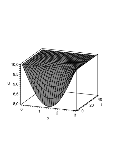
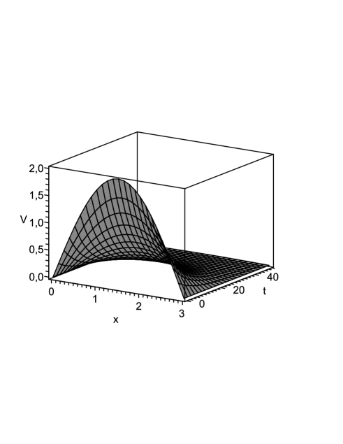
Figure 1: Solution (139) of system (138) with $a_{1}=1,\ a_{2}=2,\ \lambda_{1}=11,\ \lambda_{2}=1,\ b=0.1,\ c=0.1,\ \ C_{2}=0.2,\ \beta=~{}-0.1.$

Example. Consider solution (118) with $C_{1}=0$. Using substitution $u=-bU,\ v=-cV\ (b>0,\ c>0),$ one transforms DLV system (48) to the system describing the competition of two species

$$\begin{array}[]{l}\lambda_{1}U_{t}=U_{xx}+U(a_{1}-bU-cV),\\ \lambda_{2}V_{t}=V_{xx}+V(a_{2}-bU-cV)\end{array}$$ (138)

and solution (118) to the form

$$\begin{array}[]{l}\vskip 6.0pt plus 2.0pt minus 2.0ptU(t,x)=\frac{a_{1}}{b}+\frac{1}{(a_{1}-a_{2})b}\ C_{2}\sin(\sqrt{-\beta\lambda_{1}}x)e^{\beta t},\\ V(t,x)=\frac{1}{(a_{2}-a_{1})c}\ C_{2}\sin(\sqrt{-\beta\lambda_{1}}x)e^{\beta t},\end{array}$$ (139)

where the coefficient restrictions $\beta\equiv\frac{a_{1}-a_{2}}{\lambda_{1}-\lambda_{2}}<0,\ a_{1}>0,\ a_{2}>0$ are assumed. Using this solution one may formulate the following theorem giving the classical solution for the BVP with the constant Dirichlet conditions on the boundaries.

Theorem 4

The classical solution of boundary-value problem for the competition system (138) and the initial profile

$$\begin{array}[]{l}\vskip 6.0pt plus 2.0pt minus 2.0ptU(0,x)=\frac{a_{1}}{b}+\frac{1}{(a_{1}-a_{2})b}\ C_{2}\sin(\sqrt{-\beta\lambda_{1}}x),\\ V(0,x)=\frac{1}{(a_{2}-a_{1})c}\ C_{2}\sin(\sqrt{-\beta\lambda_{1}}x),\end{array}$$ (140)

and boundary conditions

$$\begin{array}[]{l}x=0:\ U=\frac{a_{1}}{b},\ V=0,\\ x=\frac{\pi}{\sqrt{-\beta\lambda_{1}}}:\ U=\frac{a_{1}}{b},\ V=0,\end{array}$$ (141)

in domain $\Omega=\{(t,x)\in(0,+\infty)\times\Bigl{(}0,\frac{\pi}{\sqrt{-\beta\lambda_{1}}}\Bigr{)}\}$ is given by formulae (139).

The solution (139) with $\beta<0$ has the time asymptotic

$$(U,\ V)\rightarrow(\frac{a_{1}}{b},\ 0),\quad t\rightarrow+\infty.$$ (142)

Thus, this solution describes the competition between the two species when the species $U$ eventually dominate while the species $V$ die. An example of this competition with the correctly-specified coefficients is presented on Fig.1.

5. Conclusions

In this paper $Q$-conditional symmetries of the diffusive Lotka-Volterra system (2) and their application for finding exact solutions are studied. Following the recent paper [27], two different definitions of such symmetries are used to derive systems of DEs and to construct them in the explicit form. It turns out that $Q$-conditional operators of the first type can be derived much easier than those of the second type (nonclassical symmetries), hence, Theorem 3 was proved, which completes description of $Q$-conditional operators of the first type. Nevertheless Theorem 1 presents a wider list of $Q$-conditional operators (because all the operators of the first type are automatically among those of the second type), the result is still incomplete. In fact, the additional restriction on the form of operators in question was used.

All the $Q$-conditional operators obtained were used to construct non-Lie ansätze and to reduce DLV system (2) to the corresponding systems of ODEs. As result, a wide range of new exact solutions in explicit form was found. These solutions possess a complicated structure and cannot be found by the classical Lie algorithm. In the particular case, they differs from the standard plane wave solutions obtained in [9, 30]. Note plane wave solutions can be derived from some ansätze listed in Table 1 under additional restrictions (see, e.g., ansätze with $\varphi_{1}=const$ in 3-rd and 4-th cases of the table).

Finally, a realistic interpretation for competing species has been provided for exact solution (139). In fact, this solution describes the competition between two populations of species when one of them eventually leads to the extinction of other.

The work is in progress to construct $Q$-conditional symmetries and exact solutions of a multicomponent DLV system.

References

• [1] A.M. Turing, The chemical basis of morphogenesis, Phil. Trans. Roy. Soc. Lond. 237 (1952) 37-72.
• [2] R. Cherniha, J.R. King, Lie Symmetries of Nonlinear Multidimensional Reaction-Diffusion Systems I, J. Phys. A 33 (2000) 267-282, 7839–7841.
• [3] R. Cherniha, J.R. King, Lie Symmetries of Nonlinear Multidimensional Reaction-Diffusion Systems II, J. Phys. A 36 (2003) 405-425.
• [4] A.G. Nikitin, Group classification of systems of non-linear reaction-diffusion equations, Ukrainian Math. Bull 2 (2005) 153-204.
• [5] W.F. Ames, Nonlinear Partial Differential Equations in Engineering, Academic Press, New York, 1972.
• [6] J.D. Murray, Mathematical Biology, Springer, Berlin, 1989.
• [7] N.F. Britton, Essential Mathematical Biology, Springer, Berlin, 2003.
• [8] A. Okubo, S.A. Levin, Diffusion and Ecological Problems, Modern Perspectives, second ed., Springer, Berlin, 2001.
• [9] R. Cherniha, V. Dutka, A diffusive Lotka-Volterra system: Lie symmetries, exact and numerical solutions, Ukrainian Math. J. 56 (2004) 1665-1675.
• [10] R. Cherniha, O. Pliukhin, New conditional symmetries and exact solutions of reaction-diffusion systems with power diffusivities, J. Phys. A 41 (2008) 185208-185222.
• [11] W.I. Fushchych, W.M. Shtelen, M.I. Serov, Symmetry analysis and exact solutions of equations of nonlinear mathematical physics, Kluwer, Dordrecht, 1993.
• [12] M.C. Nucci, Symmetries of linear, $C$-integrable, $S$-integrable and nonintegrable equations and dynamical systems, Nonlinear evolution equations and dynamical systems, World Sci. Publ., River Edge, (1992) 374-381.
• [13] P.A. Clarkson, E.L. Mansfield, Symmetry reductions and exact solutions of a class of nonlinear heat equations, Phys. D 70 (1993) 250-288.
• [14] D.J. Arrigo, P. Broadbridge, J.M. Hill, Nonclassical symmetry reductions of the linear diffusion equation with a nonlinear source, IMA J.Appl.Math. 52 (1994) 1-24.
• [15] D.J. Arrigo , J.M. Hill, Nonclassical symmetries for nonlinear diffusion and absorption Stud. Appl.Math. 94 (1995) 21-39.
• [16] E. Pucci, G. Saccomandi, Evolution equations, invariant surface conditions and functional separation of variables, Phys. D 139 (2000) 28-47.
• [17] R. Cherniha, M.I. Serov, Symmetries, Ansätze and Exact Solutions of Nonlinear Second-order Evolution Equations with Convection Term, Euro. J. Appl. Math. 9 ( 1998) 527–542.
• [18] R. Cherniha, New $Q$-conditional Symmetries and Exact Solutions of Some Reaction-Diffusion-Convection Equations Arising in Mathematical Biology, J. Math. Anal. Appl. 326 (2007) 783–799.
• [19] R. Cherniha, O. Pliukhin, New conditional symmetries and exact solutions of nonlinear reaction-diffusion-convection equations, J. Phys. A 40 (2007) 10049-10070.
• [20] J.M. Dixon, J.A. Tuszynski, P.A. Clarkson, From Nonlinearity to Coherence, Clarendon Press, Oxford, 1997.
• [21] B.H. Bradshaw-Hajek, P. Broadbridge, A robust cubic reaction-diffusion system for gene propagation, Math. Comput. Modelling 39 (2004) 1151-1163.
• [22] P. Olver, Applications of Lie Groups to Differential Equations, Springer, Berlin, 1986.
• [23] G.W. Bluman, S. Kumei, Symmetries and Differential Equations, Springer, Berlin, 1989.
• [24] G.W. Bluman, J.D. Cole, The general similarity solution of the heat equation, J. Math. Mech. 18 (1969) 1025-1042.
• [25] S. Murata, Non-classical symmetry and Riemann invariants, Internat. J. Non-Linear Mech. 41 (2006) 242-246.
• [26] R. Cherniha, M. Serov, Nonlinear Systems of the Burgers-type Equations: Lie and $Q$- conditional Symmetries, Ansätze and Solutions, J. Math. Anal. Appl. 282 ( 2003) 305-328.
• [27] R. Cherniha, Conditional symmetries for systems of PDEs: new definition and its application for reaction-diffusion systems. ArXiv:1005.3736v1[math-ph] 20 May 2010.
• [28] H. Beteman, Higher transcendental functions, Vol. III, McGraw-Hill, New York, 1955.
• [29] A.D. Polyanin , V.F. Zaitsev, Handbook of exact solutions for ordinary differential equations, CRC Press Company, Boca Raton, 2003.
• [30] M. Rodrigo, M. Mimura, Exact solutions of a competition-diffusion system, Hiroshima Math. J. 30 (2000) 257–270.