0cm part [0cm] chapter [1.25cm] []1.25cm  *[.5pc].  section [1.25cm] []1.25cm subsection [1.25cm] []1.25cm  *[.5pc].  figure [1.25cm]      *[.5pc].  table [1.25cm]      *[.5pc].  lchapter [0em] []1.25cm  *[.5pc].  lsection [0em] []1.25cm lsubsection [.5em] []1.25cm

Copyright © 2022 Amir Shachar

Published by Amir Shachar

https://www.amirshachar.com

All rights reserved. No portion of this book may be reproduced in any form without permission from the publisher, except as permitted by U.S. copyright law.

For permissions contact: contact@amirshachar.com

Cover by Trio Studio

First printing, April 2022

To my loved parents:Sarit, who always believed;Yaron, who used to doubt;Both ingredients were equally essential.

Part I Prologue

Chapter 1 Introduction

In the past couple of decades, trends calculations have become increasingly valuable across the scientific literature. Scientists, engineers, mathematicians, and teachers often find the derivative sign a good enough measurement of the local monotonicity. They knowingly and deliberately spare the complete information in the tangent slope and focus on its trend. Is the function ascending, descending, or constant? Humans and computer algorithms alike are increasingly asking this simple question at the core of several cutting-edge applications in multiple fields of study. For example, AI researchers are increasingly applying emerging “sign” back propagation techniques that rely solely on the loss function’s derivative sign, mathematicians are extensively investigating locally monotone operators, and chemical engineers are using Qualitative Trend Analysis to classify process monotonicity across intervals.

Unfortunately, while it is a reasonable enough estimate in most real-life and engineering applications, the derivative sign comes with inherent differentiation caveats that sometimes render it suboptimal. In continuous domains, for instance, differentiability is a must. We cannot apply the derivative at singularity points like cusps and discontinuities. Furthermore, the derivative sign often does not describe the local trend coherently at a local extremum point, where it is zeroed, but the function is not necessarily constant. Also, there is an inherent redundancy in calculating the derivative sign of functions’ quotient.

The acknowledgment of the importance of trends calculation motivates us to explore what seems to be a trend of exploiting the trend - where new theories emerge that inherently involve merely the information about functions’ trends. We take a close look at workarounds that scientists have applied to differentiation caveats in multiple scenarios. We show that researchers often spare the division operator and directly calculate the sign of the one-sided difference when evaluating trends based on discrete derivatives. We argue that avoiding the division may spare up to 20% of the runtime in this discrete implementation while maintaining the trend value. Next, we will introduce a new Calculus operator (“Detachment”) designated to measure trends, which we believe is a natural step toward modeling the workarounds that engineers have already been applying that would further improve trends estimates. Finally, we will propose a mathematical theory emerging from the novel trend operator: Semi-discrete Calculus.

1.1 How to Read This Book

The book is comprised of three main parts: Part II introduces "Trendland", where we review previous works on local trends in the form of cherry-picked articles from the relevant scientific literature. For each paper, we highlight the application of the trend within the algorithmic or scientific framework. Part III discusses several scientific aspects of the papers reviewed in Trendland, along with a review of known issues in the definition of trend as the derivative sign and emerging workarounds. Part IV defines some of the recent workarounds as a standalone mathematical operator and proposes a mathematical theory based on it.

Note that part II (Trendland) is meant to convey the message that trends calculations are becoming excessive in the scientific literature. It is not meant to be read as-is but rather skim through and focus on the reader’s interest areas. For instance, AI researchers will probably find most interest in subsection 2.1.1, which is part of the engineering Trendland, chemical physicists are likely to find more valuable information in subsubsection 3.6.1.1, which is part of the scientific Trendland, and teachers will likely find interest in the educational Trendland portrayed in chapter 5. While part III is intended for scientists, engineers and mathematicians alike, it is likely that the mathematical discussion in part IV will be of particular interest to mathematicians and scientists.

Nomenclature

The indicator function of the set $A$

The partial derivative of $f$ (with respect to $x$)

The multiple integral of $f$ in the domain $D$

The definite integral of $f$ in the interval $\left[a,b\right]$

The signum of $x$: $-1$ if $x<0$, $0$ if $x=0$, $+1$ if $x>0$

The first derivative of $f$ (with respect to $x$)

An antiderivative of $f$

The detachment of $f$

The $n^{\text{th}}$ derivative of $f$

Complex numbers

Natural numbers

Rational numbers

Real numbers

Integers

Part II Previous Work - Trendland

Chapter 2 The Engineering Trendland

In this chapter, we will see several examples of the use of the derivative sign in computer science and engineering, as well as electrical, systematic, mechanical, civil, agricultural, quantum, and aerospace engineering.

2.1 Computer Science and Engineering

2.1.1 Machine Learning

2.1.1.1 Machine Learning Optimization

While the gradient is the fundamental concept in many optimization algorithms, it turns out that its sign is an essential stand-alone component in some of them. Recently, several papers pointed out this trend in the literature and surveyed several algorithms that incorporate the derivative sign while analyzing their mathematical and convergence properties ([992, 683]). Let us study examples of optimization algorithms in which the derivative’s sign was found lucrative to researchers due to its relative stability.

Researchers often treat the RProp ([815]) algorithm as a basis for other optimization approaches relying on the derivative sign. Although originated in 1993, researchers still cite the approach proposed by Riedmiller and Braun as one of the recommended optimization frameworks, alongside its modern alternatives - even when it comes to deep learning optimization. For example, [93] recommends it, and [994] states that this unique formalization allows the gradient method to overcome some cost curvatures that we may not solve quickly with today’s dominant methods.

The two-decade-old method is still worthy of our consideration. We can formulate the algorithm as follows:

$$\theta^{t+1}=\theta^{t}-\eta_{+}I\left(sgn\left(\frac{\partial L}{\partial\theta}\left(\theta^{t}\right)\right)>0\right)+\eta_{-}I\left(sgn\left(\frac{\partial L}{\partial\theta}\left(\theta^{t}\right)\right)<0\right),$$

Where $I(\cdot)$ is the indicator function. Based on the gradient sign, we decide to proceed with a growing or shrinking step size in each iteration. In other words, in case the optimizee trends upwards, then to reach the minimum, our step should be of size $\eta^{+}$ to the left, and vice versa. The sizes of the steps vary exponentially, allowing for efficient exploration and a binary search based exploitation.

Let us gain some intuition regarding this algorithm’s efficiency. We can think of optimization as a prediction task in which we impose an intelligent guess of a lucrative step towards an optimum. Intuitively, the magnitude of the gradient seems like a reasonable consideration. However, often – for example, in cases where the function’s rate of change plunges – a simple binary search may land on the optimum faster. Another way to think about it is that the gradient’s magnitude might ’overfit’ the optimizer’s prediction relative to the sign alone. In other words, as a function increases, a step in the negative direction is guaranteed to promote us towards a local minimum. However, one can only speculates about a correct way to rely on the gradient’s magnitude for the step size, and speculations are often inaccurate and give rise to challenging scientific debate.

In [93], for instance, RProp mitigates the challenge of vanishing gradients, as it overlooks their magnitude. However, RProp entails a considerable challenge. It renders the optimization method discontinuous upon conducting SGD. For example, imagine that some mini-batches dictate a gradual deterioration of the gradient. Suppose we proceed with a mini-batch whose gradient cancels the previous ones. The researcher would expect the steps themselves to balance out and that the optimization process would end up where it began, which is the case in Stochastic Gradient Descent methods. In contrast, the described case renders RProp proceed without canceling out the accumulated gradients.

Other optimization algorithms leverage the gradient’s sign only implicitly, including AdaGrad ([616]), AdaDelta ([1042]) and RMSProp ([435]). In such algorithms, we divide by the weighted root of the mean squares of the previous gradients. We can think of this standardization as a generalization of RProp in that it considers the sign of the current gradient while doing it smoothly relative to the process thus far, which is evident when we restrict the window size to include only the most recent gradient. The gradient’s magnitude in the numerator then cancels out with its absolute value in the denominator, resulting in the gradient’s sign.

An alternative to this type of algorithms is an emerging family of machine learning (ML) algorithms that use the derivative sign explicitly. They are referred to in the literature as the “Sign” algorithms. Thus, researchers often refer to RProp as the signed gradient descent; SignSGD is a version of stochastic gradient descent that applies its sign, SignAdam is the analog of Adam, and so on.

Several proposals on how to further improve the RProp algorithm have been made, including the work of [462], which focuses on the loss function’s local trends and proposes a modifications of the original algorithm that improves its learning speed.[42] introduces an efficient modification of the Rprop algorithm for training neural networks and proposes three conditions that any algorithm that employs information of the sign of partial derivative should fulfill to update the weights.

Quickprop ([827]) proposes looking at the evolution of the sign of the gradient with respect to one parameter for successive iterations; if it is the same, one should follow the gradient descent direction; if it is different, a minimum is likely to exist in between the preceding and current values and one should expect to be in a situation where the second-order approximation is reasonable.

[240] introduces the normalized and signed gradient descent flows associated with a differential function. The flows characterize their convergence properties via non-smooth stability analysis. They also identify general conditions under which these flows attain the set of critical points of the function in a finite time. To do this, they extend the results on the stability and convergence properties of general non smooth dynamical systems via locally Lipschitz and regular Lyapunov functions.

[1037, 790, 691] discuss the pros and cons of RProp and compare several approaches for backpropagation that leverage the derivative sign. Among them are "Sign Changes," "Delta-bar-delta," "RProp," "SuperSAB," and "QuickProp."

A key challenge in applying model-based Reinforcement Learning and optimal control methods to complex dynamical systems, such as those arising in many robotics tasks, is the difficulty of obtaining an accurate system model. These algorithms perform very well when they are given or can learn an accurate dynamics model. However, it is often very challenging to build an accurate model by any means: effects such as hidden or incomplete state, dynamic or unknown system elements, and other effects, can render the modeling task very difficult.

[540] presents methods for dealing with such situations by proposing algorithms that can achieve good performance on control tasks even using only inaccurate system models. In particular, one of the algorithmic contributions that exploit inaccurate system models is an approximate policy gradient method, based on an approximation called the Signed Derivative, which can perform well when only the sign of specific model derivative terms are known.

In a study focusing on the associations between the fields of active learning and stochastic convex optimization, [803] proposes an algorithm that solves stochastic convex optimization using only noisy gradient signs by repeatedly performing Active Learning, achieves optimal rates, and is adaptive to all unknown convexity and smoothness parameters.

[1044] proposes an algorithm which utilizes a greedy coordinate ascent algorithm that maximizes the average margin over all training examples, leveraging the derivative sign in an interval.

[363] introduces, Gradient reverse layer (GRL), an identity transformation in forward propagation that changes the sign of the gradient in backward propagation.

[1038] proposes that we update the weights by only using sign information of the classical backpropagation algorithm in the Manhattan Rule training. Equations 3.4, 3.5 in [998] state that the partial derivatives of $y^{\prime}$ equal the sign of the derivatives of $w$ and $x$, respectively.

Parallel implementations of stochastic gradient descent (SGD) have received significant research attention, thanks to its excellent scalability properties. A fundamental barrier when parallelizing SGD is the high bandwidth cost of communicating gradient updates between nodes; consequently, researchers have proposed several lossy compression heuristics, by which nodes only communicate quantized gradients. Although effective in practice, these heuristics do not always converge.

An interesting example of parallel implementations of SGD is the work of [31], who propose Quantized SGD (QSGD), a family of compression schemes with convergence guarantees and good practical performance. The "ternarize" operation in Eq. 1 of [1007] splits the gradient to its sign and magnitude ingredients. The parameter in TernGrad is upgraded in turn by Eq. 8, where the gradient sign is applied. Theorem 1 then proves a convergence property of this gradient sign-based algorithm.

Backpropagation provides a method for telling each layer how to improve the loss. Conversely, in hard-threshold networks, target propagation offers a technique for telling each layer how to adjust its outputs to enhance the following layer’s loss. While gradients cannot propagate through hard-threshold units, one may still compute the derivatives within a layer. As illustrated in [351], an effective and efficient heuristic for setting the target activation layer is to use the (negative) sign of the partial derivative of the next layer’s loss.

Training large neural networks requires distributing learning across multiple workers, where the cost of communicating gradients can be a significant bottleneck. SignSGD alleviates this problem by transmitting just the sign of each minibatch stochastic gradient. [115] proves that it can get the best of both worlds: compressed gradients and SGD-level convergence rate. The relative $\ell_{1}$ or $\ell_{2}$ geometry of gradients, noise, and curvature informs whether signSGD or SGD is theoretically better suited to a particular problem. On the practical side, the authors find that the momentum counterpart of signSGD can match the accuracy and convergence speed of ADAM on deep Imagenet models.

[71] interprets ADAM as a combination of two aspects: for each weight, the update direction is determined by the sign of stochastic gradients, whereas an estimate of their relative variance determines the update magnitude; they disentangle these two aspects and analyze them in isolation, gaining insight into the mechanisms underlying ADAM.

[1049] propose an algorithm based on the derivative sign of the backpropagation error. [114] further studies the base theoretical properties of this simple yet powerful SignSGD. The authors establish convergence rates for signSGD on general non-convex functions under transparent conditions. They show that the rate of signSGD to reach first-order critical points matches that of SGD in terms of the number of stochastic gradient calls but loses out by roughly a linear factor in the dimension for general non-convex functions.

[1000] explores the usage of a highly low-precision gradient descent algorithm called SignSGD. The original algorithm still requires complete gradient computation and therefore does not save energy. The authors propose a novel "predictive" variant to obtain the sign without computing the full gradient via low-cost, bit-level prediction. Combined with a mixed-precision design, this approach decreases both computation and data movement costs.

[683] studied the properties of the sign gradient descent algorithms involving the sign of the gradient instead of the gradient itself. This article provides two convergence results for local optimization, the first one for nominal systems without uncertainty and a second one for uncertainties. New sign gradient descent algorithms, including the dichotomy algorithm DICHO, are applied on several examples to show their effectiveness in terms of speed of convergence. As a novelty, the sign gradient descent algorithms can converge in practice towards other minima than the closest minimum of the initial condition, making this new metaheuristic method suitable for global optimization as a new metaheuristic method.

[992] applies the sign operation of stochastic gradients (as in sign-based methods such as signSGD) into ADAM, called signADAM. This approach is easy to implement and can speed up the training of various deep neural networks. From a computational point of view, choosing the sign operation is appealing for the following reasons:

• Tasks based on deep learning, such as image classification, usually have a large amount of training data. "Training" on such a data set may take a week, even a month, to shrink calculation in every step, enhancing efficiency.

• The algorithm can induce sparsity of gradients by not updating some of the gradients. One of the ADAM’s drawbacks is that it ignores these gradients by using the exponential average algorithm. SignAdam++ can prevent this issue by giving small gradients shallow confidence (e.g., $0$).

• Nowadays, learning from samples in deep learning is always stochastic due to the massive amount of data and models. The confidence of some gradients produced by loss functions should be small. From the perspective of the maximum entropy theory, each feature should have the equal right to make efforts in a deep neural network.

• The incorrect samples cause large gradients which may hurt the models’ generalization and learning ability. signADAM++ addresses this issue by using moving averages after applying confidence for unprocessed gradients and an adaptive confidence for some large gradients; hence, improving the performance in some models.

As illustrated in [502], sign changes in the directional derivative along a search direction may appear and disappear stochastically as the oracle updates the mini-batches. In addition to the sign change of each mini-batch loss function, additional sampling-induced sign changes may manifest along a search direction. This occurs when the oracle switches between a negative and positive directional derivative for essentially the same step along a search direction. [791] argues that only the signs of the gradients would amplify small noisy gradients, making the conformity score not useful. Instead, CProp measures the conformity by asking the following:" Does the past gradients conform enough to show a clear sign, positive or negative collectively?"

[207] argues in favor of the Gradient Sign Dropout (GradDrop) method, noting that when multiple gradient values try to update the same scalar within a deep network, conflicts arise through differences in sign between the gradient values. Following these gradients blindly leads to gradient tugs-of-war and to critical points where constituent gradients can still be significant,making some tasks perform poorly. [207] demand that all gradient updates are pure in sign at every update position to alleviate this issue. Given a list of (possibly) conflicting gradient values, the method proposed algorithmically selects one sign (positive or negative) based on the distribution of gradient values and mask out all gradient values of the opposite sign.[493] applies directional derivative signs strategically placed in the hyperparameter search space to seek a more complex model than the one obtained with small data.

[14] explored whether one can generate an imperceptible gradient noise to fool the deep neural networks. For this, the authors analyzed the role of the sign function in the gradient attack and the role of the direction of the gradient for image manipulation. When one manipulates an image in the positive direction of the gradient, they generate an adversarial image. On the other hand, if they utilize the opposite direction of the gradient for image manipulation, one observes a reduction in the classification error rate of the CNN model.

In [617], the signSGD flow, which is the limit of Adam when taking the learning rate to $0$ while keeping the momentum parameters fixed, is used to explain the fast initial convergence.

Sign-based optimization methods have become popular in machine learning also due to their favorable communication cost in distributed optimization and their surprisingly good performance in neural network training. [72], for instance, finds sign-based methods to be preferable over gradient descent if the following conditions are met:

• The Hessian is to some degree concentrated on its diagonal

• Its maximal eigenvalue is much larger than the average eigenvalue

  Both properties are common in deep networks

[837] analyzed sign-based methods for non-convex optimization in three key settings: Standard single node, parallel with shared data, and distributed with partitioned data. Single machine cases generalize the previous analysis of signSGD, relying on intuitive bounds on success probabilities and allowing even biased estimators. Furthermore, this work extended the analysis to parallel settings within a parameter server framework, where exponentially fast noise reduction is guaranteed with respect to the number of nodes, maintaining 1-bit compression in both directions and using small mini-batch sizes. Next, they identified a fundamental issue with signSGD to converge in a distributed environment. To resolve this issue, they propose a new sign-based method, Stochastic Sign Descent with Momentum (SSDM), which converges under standard bounded variance assumption with the optimal asymptotic rate.

Due to its simplicity, the sign gradient descent is popular among memristive neuromorphic systems. When implementing it with memristor synapses, as in [279], the LB sends a single UP (or DOWN) pulse to instruct an increase (or decrease) of the synaptic weights. Hence, a single SET pulse is applied to the PCM device, determined by the gradient sign. However, the effective value of $\delta$ is not constant due to the WRITE noise and is not symmetric because SET operation in PCM is gradual, whereas RESET is abrupt.

[600] investigated faster convergence for a variant of sign-based gradient descent, called scaled signSGD, in three cases:

• The objective function is firmly convex

• The objective function is non-convex but satisfies the Polyak-Łojasiewicz (PL) inequality

• The gradient is stochastic, called scaled signSGD in this case.

  [1061] studied the optimization behavior of signSGD and then extend it to Adam using their similarities; Adam behaves similarly to sign gradient descent when using sufficiently small step size or the moving average parameters $\beta_{1}$,$\beta_{2}$ are nearly zero.

2.1.1.2 Adversarial Learning

One of the simplest methods to generate adversarial images (FGSM) is motivated by linearizing the cost function and solving for the perturbation that maximizes the cost subject to an $\ell_{\infty}$ constraint. Based on the gradient sign, one may accomplish this in closed form for the cost of one call to back-propagation. In [560], this approach is referred to as "fast" because it does not require an iterative procedure to compute adversarial examples and thus it is much faster than other considered methods.

Several other approaches have been proposed for fast adversial learning.[560], for instance, introduce a straightforward way to extend the "fast" method — they apply it multiple times with small step size and clip pixel values of intermediate results after each step to ensure that they are in an $\varepsilon$-neighbourhood of the original image.

To achieve a rapid generation of adversarial examples in the "Fast Gradient Sign" algorithm,[391]applies the sign of loss function’s derivative with respect to the input.

[672] add a perturbation to Neural networks to fool them with the DeepFool algorithm. The authors used the sign of the derivative in the iterative update rule with the supremum norm. They also apply the fast gradient sign method, wherein the absence of general rules to choose the parameter $\varepsilon$, they chose the smallest $\varepsilon$ such that $90\%$ of the data are misclassified after perturbation.

[747]crafts an adversarial sequence for the Long Short-Term Memory (LSTM) model. The algorithm iteratively modifies words in the input sentence to produce an adversarial sequence. The LSTM architecture then misclassifies it. The optimization step applies the sign of the gradient $J$.

[952] visualizes the “gradient-masking” effect by plotting the loss of $v_{adv}^{3}$ on examples $x^{\ast}=x+\varepsilon_{1}\cdot g+\varepsilon_{2}\cdot g^{\bot}$, where $g$ is the signed gradient of model $v_{adv}^{3}$ and $g^{\bot}$ is the assigned vector orthogonal to $g$. In Section 4.1, they chose $g^{\bot}$ to be the signed gradient of another Inception model, from which adversarial examples transfer to $v_{adv}^{3}$. In appendix E, properties regarding the gradient-aligned adversarial subspaces for the $\ell_{\infty}$ norm utilize the signed gradient (lemmas 6, 7).

[622] lays the foundation of a widespread attack method - the PGD (projected gradient descent) attack described in section 2.1. This method uses just the sign of the gradient. Since its discovery, the superiority of signed gradients to raw gradients for producing adversarial examples has puzzled the robustness community. Still, these strong gradient signal fluctuations could help the attack escape suboptimal solutions with a low gradient.

The sign of the partial derivative of $J^{\prime}$ in [618] is defined as a standalone operator in equation 6 and applied to solve the second problem using a bounded update approach. In turn, lemma 1 proves a bound on a number defined based on the derivative sign.

Selecting $\mu=0$ in Eq. 6 of [295] yields, in turn, the I-FGSM, with the gradient sign as the update direction. Otherwise, the sign is applied to an approximation of the gradient.

The fast gradient sign method is tweaked in several aspects. One of them is that the algorithm in [846], which performs backward pass using the classification loss function. Each gradient accumulation layer Gc stores the gradient signal backpropagated to that layer via its sign (Eq. 5 there).

[1020] surveys the performance of extensions of the fast gradient sign method and proposes the method $M-DI^{2}-FGSM$, whose special cases are $DI^{2}-FGSM$ and $MI-FGSM$ - all of which leverage the gradient sign for some constellations of parameters.

Cheng et al. propose an approach for hard-label black-box attack which models hard-label attack as an optimization problem where the objective function can be evaluated by binary search with additional model queries. Thereby, a zeroth-order optimization algorithm can be applied. In [212], the authors adopt the same optimization formulation; however, they suggest to directly estimate the sign of the gradient in any direction instead of the gradient itself, which benefits a single query. By using this single query oracle for retrieving the sign of directional derivative, they develop a novel query-efficient Sign-OPT approach for a hard-label black-box attack.

Combined with the fast sign gradient method, [365] proposes the Patch-wise Iterative Fast Gradient Sign Method (PI-FGSM) to generate strongly transferable adversarial examples. The authors surveyed the development of the gradient sign-based attack method in section 3.1 and their algorithm also applies the loss function’s gradient sign.

The adversarial bracketed exposure fusion-based attack in Eq. 6 of [214] is optimized with the sign gradient descent (Eq. 9 there).

In [604], given a clean input image and a pre-trained DNN, Differential Evolution first derives a gradient sign population, children candidates competes with their parents using the corresponding perturbed inputs and, finally, the authors perturbed the inputs with the approximate gradient signs.

In the proof of the proposition in [346], it is only required to look at the sign of the derivative of "$\alpha$" for some arbitrary perturbation $\Delta_{j}^{\ast}$. Then, because the crafting algorithm uses signed gradient descent (either Adam or SGD), the perturbations crafted using the online vs. non-online method will be identical.

In [373], it is possible to optimize the adversarial perturbation through projected descent (PGD) for all attacks. The authors found Signed Adam, with a step size of 0.1, a robust first-order optimization tool to this end. While perturbation bounds were weakly enforced in the original version by an additional penalty, the authors optimized the objective directly by projected (signed) gradient descent in line with other attacks. They find this approach to be at least equally effective. The proposed method implements specific adversarial training at training steps, starting from a randomly initialized perturbation and maximizing cross-entropy for five steps via signed descent. Further, it optimizes the surrogate attacks via signed Adam descent with the same parameters described in the attack section.

The stronger the anti-adversary layer solver for Problem (2) in [29] is, the more robust $g$ is against all attacks. To that end, the anti-adversary layer solves Problem (2) with $K$ signed gradient descent iterations, zero initialization, and $L$ is the cross-entropy loss. Algorithm 1 summarizes the forward pass of $g$.

[366] suggests integrating the attack method into any gradient-based additive-perturbation attack methods, e.g., FGSM, BIM, MIFGSM. The authors use the sign gradient descent optimization with the step size $\lambda=\frac{\varepsilon}{T}$. $T$ denoting the iteration number, and they fix it as ten as a typical setup in adversarial attacks.

Algorithm 1 in [739] defines the adversarial direction in the Individual AGI based on the sign of the $f$ gradient.

The “fast derivative sign” method has become so prevalent, that an analogous “derivative magnitude” method was introduced in [830], emphasizing that it is the magnitude and not merely the sign that is being exploited.

2.1.1.3 Meta-Learning

[44] presents LSTMs that can learn to conduct Gradient Descent automatically. Their model learns how to learn; it builds a favorable optimization method per each domain separately and outperforms hand-crafted optimization algorithms such as Adam. The authors mention a crucial challenge in training the optimizers: different input coordinates can have different magnitudes, which can make training an optimizer difficult because neural networks naturally disregard small variations in input signals and concentrate on bigger input values. To tackle it, the authors decided to replace the gradients by two other features: $\left(\log\left|\nabla L\right|,sgn\left(\nabla L\right)\right)$. In other words, to overcome the instability of the gradient operator, they scaled it down exponentially to a positive number and added its sign.

This approach is adopted by [806] in their prominent MAML few-shot learning framework.

2.1.1.3.1   Neural Networks

Section 6.3 of [93] discusses supervised learning for recurrent networks. The difficulty of gradient computation in recurrent networks makes it necessary to employ algorithms that use only the gradient sign to update the weights. For example, the magnitudes of the backpropagated errors may vary significantly. For this reason, it is challenging to determine a constant learning rate for gradient descent that allows for both stable learning and fast convergence. Since the RProp algorithm does not use the magnitude of the gradient, it is not affected by very small or substantial gradients. Hence, it is advisable to combine this algorithm with backpropagation through time. This training method for recurrent neural networks have been experimentally shown to avoid the stability problems of fixed-rate gradient descent while at the same time being one of the most efficient optimization methods.

[270] partitions the State-space into regions with a unique derivative sign pattern. It is shown that a qualitative abstraction yields a state transition graph that provides the discrete picture of continuous dynamics.

[844] proposed an explicitation method of gradual rules, which allows the extraction of rules starting from the ASP units. To build a MGR, the sign of the output’s derivative is analyzed, among others.

Several backpropagation methods such as SSAB, RPROP and GNFAM are characterized by using the derivative sign to increase or decrease the learning rate (LR) exponentially. These methods are surveyed in [34], who show that different problems require different learning rate adaptive methods.

Failure modes 5 & 6 in [561] refer to scenarios where the SCANN function’s derivative sign is positive or negative, which prevents the opposite of what was intended in output changes over input changes (for example, the output must increase if the input increases). The safety argument for adhering to these bounds focuses upon assuring that the derivative sign (rule function gradient) as expressed by Eq. 50 is limited during generalization and learning. The solution to this argument is that parameter $a_{i}\left(1\right)$ will always be positive to reflect increasing output and negative to define decreasing output. In addition, the gradient, in any case, can be zero as a result of the saturation performed by the rule output bounds.

[87] introduces a hyperrectangular partition of the state space that forms the basis for a discrete abstraction preserving the sign of the derivatives of the state variables. The approach defines a fine-grained partition of the state space which underlies a discrete abstraction preserving more substantial properties of the qualitative dynamics of the system, i.e., the derivative sign pattern.

Among the hand-chosen features in a work on fast classification and anomaly measurement, [1014], the Normalized Decay describes the chance-corrected fraction of data that is decreasing or increasing based on the sign of the discrete derivative.

The lecture in [435] introduces the RMSProp algorithm. The gradient is divided by the (weighted) root of the mean squares of the gradients in the proceeding steps. One may view this standardization as a generalization of RProp in that it considers the sign of the current gradient smoothly with respect to the process thus far. The gradient’s magnitude in the numerator cancels out with its absolute value in the denominator, resulting in the gradient’s sign.

At the deep neural net studied in [782],the number of times a single neuron has a sign change in the derivative across the parameters serves as a crucial upper bound for exponential expressivity.

To identify whether a given data point $x$ is a critical sample, [51] searches for an adversarial example within a box of a given radius. To perform this search, the authors use Langevin dynamics applied to the fast gradient sign method as shown in algorithm 14. They refer to this method as Langevin adversarial sample search (LASS). While the FGSM search algorithm can get stuck at a point with zero gradients, LASS explores the box more thoroughly. Specifically, a problem with first-order gradient search methods (like FGSM) is that there might exist training points where the gradient is $0$, but with a large $2^{nd}$ derivative corresponding to a significant change in prediction in the neighborhood. The noise added by the LASS algorithm during the search enables escaping from such points.

[994] argues that RProp’s (signed gradient descent) unique formalization allows the gradient method to overcome some cost curvatures that may not be easily solved with today’s dominant methods, depending on the problem’s geometry.

[455] introduce a method to train Quantized Neural Networks (QNNs) — neural networks with extremely low precision (e.g., 1-bit) weights and activations at run-time. At train-time, the quantized weights and activations are used for computing the parameter gradients. QNNs drastically reduce memory size and accesses during the forward pass and replaces most arithmetic operations with bit-wise operations. As a result, power consumption is expected to be drastically reduced.

[324] applies the sign of the loss function’s gradient to prove theorem 16. The results are reflected in the update in algorithm 3.

As explained in [359], if the loss function’s derivative is positive, then an increase or decrease in the weight increases or decreases the error, respectively; the opposite effects occur if the derivative is negative.

In [378], the gradient sign of the dissimilarity function that measures the change between the interpretations of two images is applied to iterative feature importance attacks.

[397] analyzes the sensitivity of the cause-and-effect relations. The first partial derivative of the regression function is computed with respect to each input parameter. A significant value of the partial derivative indicates a considerable influence of the corresponding input parameter, i.e., small changes in the input will lead to substantial changes in the output. Furthermore, the sign of the partial derivative is essential. A positive partial derivative indicates that an increase in the input leads to a rise in output. A negative sign means that an increase in the input leads to a decrease in the output.

To overcome the vanishing gradient problem, [7] introduced a new anti-vanishing back-propagated learning algorithm called oriented stochastic loss descent (OSLD). OSLD updates a random-initialized parameter iteratively in the opposite direction of its partial derivative sign by a small positive random number, which is scaled by a tuned ratio of the model loss.

In [421], the backward gain w.r.t w is $\beta=\frac{\partial y^{\prime}}{\partial w}=\sigma x$ where $\sigma$ is the gain of the activation function $\sigma$. If input $x$ is negative or $\sigma$ is negative, $\beta$ is negative, and $A\beta$ becomes negative, which is unstable. To make the system stable for negative backward gain, the forward gain $A$ needs to be negative so that $A\beta$ becomes positive. The output of the backward function for negative $\beta$ can be expressed as (10). We can transfer the negative sign to the error $e$ and keep $A$ positive. Since the negative sign is there because of the negative backward gain $\beta$, the sign can be replaced by the signum function as in (12). For negative backward gain, we can continue using positive forward gain with the error $e$ augmented by the sign of the backward gain. For positive backward gain, no negative sign is necessary. Thus (12) is consistent for both positive and negative values of $\beta$.

2.1.1.3.2   Federated Learning

In the online learning algorithm presented by [416], we see an example of the use of an estimated sign of the derivative of the objective function which gives a regret bound that is asymptotically equal to the case where the exact derivative is available. Encrypting and decrypting all elements of the model gradients have several shortcomings. First, performing encryption on local clients is computationally extremely expensive, causing a big barrier for real-world applications since the distributed edge devices usually do not have abundant computational resources. Second, uploading model gradients in terms of cipher text incur high communication costs. Finally, the first two issues will become computationally prohibitive when the model is large and complex, e.g., DNNs.

To tackle the above challenges, [1058] introduces ternary gradient quantization (TernGrad) into their federated learning framework. TernGrad compresses the original model gradients into ternary precision gradients with values $\in\left\{-1,0,1\right\}$ as described in Eq. (13)..

In the signed gradient scenario of [623], computing the gradient of the objective in (7) involves finding the sign of the gradient with respect to $\left\{w_{1},w_{2},\ldots,w_{N}\right\}$ instead of the full gradient, and the full gradient with respect to $\alpha$; this provides a function of a relatively lesser dimensional information. The gradient with respect to the importance coefficients $\alpha$ does not depend on the neural network weights but on the discrepancy and the losses. The method involves sending $O\left(N\right)$ parameters while the gradient with respect to neural network weights $w$ can potentially involve millions $\left(>O\left(N\right)\right)$ of parameters. The signed gradient of the objective function (7) with respect to the weight of the device $k$ includes the sign function within the summation, as shown in (9).

The algorithm in [766] provides decentralized optimization in wireless device-to-device networks of pervasive devices such as sensors or 5G handsets. The signs of the stochastic gradient are used for descent steps.

Averaging masked gradients in [943] is equivalent to averaging the gradients directly when all the client gradients being considered are of the same sign.

2.1.1.3.3   Reinforcement Learning

In a work on policy search for reinforcement learning [541], the approximation is based on the intuition that it is often straightforward to guess the direction in which control inputs affect future state variables, even if we do not have an accurate system model.

The reward function, defined in Eq. 1 of [543], can be thought of as the sign of the discrete numerical derivative of the Intersection-over-Union (IoU) function.

The initial reward in [939] is defined as the sign of the discrete derivative of the probability function that predicts the video as belonging to a specific class across consecutive iterations.

While an optimal policy is deterministic (gradient ascent searches among all threshold policies), the gradient is discontinuous at such policies. Plain Gradient Ascent suffers from this problem. Therefore [637] suggests taking integer steps to explore just integer policies, calculate both one-sided gradients, and use them in the update step. In turn, the gradient sign is then used within this optimization method.

As shown in Algorithm 3 in [1048], when generating adversarial samples, the adversary computes the perturbation with $g_{i}=sgn\left(\frac{\partial J\left(G,y\right)}{\partial V}\right)$. $V$ is the feature matrix, each row of which describes instructions in a basic block $v_{i}$ of the graph $G$, and $y$ is the label of the CFG. The attacker heuristically inserts a semantic Nop that is closest to the gradient $g_{i}$ into the corresponding basic block of the CFG. In each iteration, the attacker injects the closet semantic nops to the sign gradient descent. The attacker then repeats this procedure until a maximum number of iterations $T$.

2.1.1.3.4   Regression

[468] derives a necessary and sufficient condition for identifying the sign of the derivative of an unknown monotonic function by the method of weighted average derivatives. While OLS has a weighted average derivative representation, it does not necessarily satisfies the condition except in restrictive cases.

As portrayed in [857], the orthant-wise learning algorithm of Andrew et al. uses a direct approach. In particular, they computed and set any value $d_{i}$ in $d$ to zero if its sign does not agree with $-\nabla f(x_{k})$, as in Eq. 2.8 . However, this algorithm does not satisfy the property of reducing to Newton’s method because of the PS sign projection. The problem with this projection is that it may set elements of the Newton direction to zero for a large portion of the zero and non-zero variables. However, to lie in the correct orthant (to guarantee descent), the only requirement is that the zero-valued variables in the search direction agree with the negative pseudo-gradient sign. Thus, in the PSS sign projection (PSSsp) variant, the authors apply the orthant-wise learning iteration but use a less constrained version of the PSsign projection, denoted by $P_{s}^{*}$.

Corollary 1 in [741] claims that if we have two roots for $f\left(x\right)=0$ on an interval and the tangent lines on the two endpoints have the same derivative direction, there must be another root between the two with a different derivative sign.

In the proof of part a of theorem 2 in [1023], it is sufficient to prove sign properties regarding the partial derivatives of $Q$ with respect to $\beta_{j}$.

2.1.1.3.5   Classification

[43] introduces a new class of sign-based schemes based on the composite nonlinear Jacobi process. An algorithm of this class that applies the bisection method to locate subminimizer approximations along each weight direction has been derived.

[332] presents a conceptually simple and computationally efficient family of texture descriptors. Three different methods have been proposed, namely single-loop, double-loop and triple-loop binary gradient contours, based on pairwise comparisons of pixel intensities all along the periphery of a $3*3$ window. These models have been comparatively analyzed from a theoretical standpoint. The Binary Gradient Contours are based on the sign of the discrete derivative of the image in different directions (Eq. 11).

Given that the traditional gradient descent algorithm suffers from long-term dependency problems, a refined BP algorithm named Rprop, which leverages the gradient’s sign solely, is extended in [206] to train multi-instance multi-label image classification (MIMLNN) effectively.

2.1.1.3.6   Computer Vision

There are many papers detailing the use of the discrete derivative sign in computer vision. The circuit in [433], for instance, is nonlinear in the sense that it produces a fairly narrow current pulse at the change of the derivative sign both for sharp and smooth inputs due to the nonlinear feedback.

[981, 999] apply the discrete derivative sign implicitly. The authors distinguish between different rectangles’ corners in the plane in efficiently calculating the integral, assigning different weights based on the corner type. Classification of corners leverages the curve’s derivative sign at its corners.

[398] found a textured print by counting the number of changes in the derivative sign in the gray level intensity function by rows and columns.

The algorithm in [701] optimizes the signal-to-noise ratio of the saliency map by scrutinizing its derivative’s sign at each iteration (Eq. 11-13).

In a work on topological mapping using spectral clustering and classification [146], one of the features used for the submap classifiers is the number of second derivative sign flips (a measure of bumpiness).

In a work on orientation-selective edge detection and enhancement using the irradiance transport equation, [343] distinguishes the sign of the derivative of the intensity pattern along an arbitrarily selected direction.

In [765], the detection of the $\left(2n+1\right)$-neighborhood maxima on a 1D scan-line is shown in detail in Figure 3a . If $g$ is the sign of the finite difference of $f,g$ is either $-1,0,$ or $1$ depending on the local slope of $f$. $g$’s finite difference $h$, therefore, equals $-2$ at local peaks, $+2$ at local troughs, and $0$ elsewhere. 1D peak and trough detection, therefore, requires only one comparison per pixel. Next, each 1D peak is compared against its $\left(2n+1\right)$-neighborhood with the knowledge of the extremum detector $h$. Neighboring pixels that are on a consecutive downward slope from the local peak are by definition more minor than the current peak. Hence they don’t need to be recompared and only pixels outside the enclosing troughs of the current peak need an extra comparison. The number of extra comparisons to obtain $\left(2n+1\right)$-neighborhood maxima from an initial list of 3-neighborhood maxima is very small for a smooth function $f$.

The method in [985], used for objects description and extraction by the use of straight line segments in digital images, includes directional filtering and searching for straight edge segments in every direction and scale, taking into account edge gradient signs.

The algorithm in [599] applies the second derivative sign to distinguish between the requirement to use Newton’s method or a line search in the optimization process while matching images observed in different camera views.

In contrast to existing approaches, the proposed cost-effective descriptors in [52] render fine orientation binning and consideration of gradient sign affordable. Experiments revealed that these descriptors achieve a significantly better trade-off between cost and performance in the vehicle verification task than standard HOG. The HOG technique was initially proposed for pedestrian detection, for which the authors claimed that including the gradient sign results in no performance gain. In effect, for humans, the wide range of clothing and background colors renders the sign of contrast uninformative. In contrast, when it comes to vehicles, the sign information might well be significant.

[809] use the sign of the numeric discrete derivative of the Euclidean distance function applied to frames to define a stop motion measure.

The derivative sign is used explicitly in a global minimization algorithm of [959] that establishes a meaningful distance between essential matrices during pose averaging.

[450] propose an iterative process to detect light streaks in the input image automatically with the sign of the derivatives of the latent image.

The computation of the second-order derivative in [1026] only considers a signed binary version of the first-order derivative.

[454] presents a computationally efficient yet powerful binary framework for robust facial representation based on image gradients (see Eq. 1,2 there)referred to as structural binary gradient patterns (SBGP). To discover underlying local structures in the gradient domain, image gradients are computed from multiple directions and simplified into a set of binary strings. The SBGP is derived from certain types of these binary strings that have meaningful local structures and resembled essential textural information. It is shown that the SBGP can detect micro-orientational edges and possess strong orientation and locality capabilities, thus enabling significant discrimination. The SBGP also benefits from the advantages of the gradient domain and exhibits profound robustness against illumination variations. The binary strategy realized by pixel correlations in a small neighborhood substantially simplifies the computational complexity and achieves extremely efficient processing.

In a study of study the problem of single-image depth estimation for images in the wild, [203] shows that adding normals improves ordinal error, but only from the angle-based normal loss, not the depth-based normal loss because depth-based normal loss emphasizes getting the same steep slopes, but this does not make any difference to ordinal error as long as the sign of the slope is correct.

In a proposed foreground-background separation [581] uses an optical phenomenon where bundles of rays from the background are flipped on their conjugate planes. Using the Lambertian assumption and gradient constraint, the foreground and background of a scene can be converted to a binary map by voting the gradient signs in every angular patch. Using light field reparameterization, the disparity map can be obtained by accumulating the binary maps.

In [566], an image is binarized using Eq. 5 . One can view it as an "or" between the signs of its partial derivatives. The process repeats seven times before the final image $g$ is calculated as a weighted average of the eight images.

According to [558], the essential part in the derivative approximation is its sign and not the amplitude because the error in the amplitude can be compensated during optimization. The algorithm in [899], for example, detects a head-turning movement in a video by assuming a frame within a short camera motion interval if the sign of all curves’ derivatives is constant at a point.

The LBDE component in [1016] describes the amplitude change among the neighborhood pixels. In Eq. 7 , the authors define the local binary gradient orientation (LBGO) to characterize the orientation information. The proposed LBGO is designed to extract gradient orientation from center-symmetric pixel pairs. Compared to the original WLD, LBGO uses the neighboring pixels and retains more local structure information.

The method proposed by [289] is interested in the general orientation of the gradient and not in the exact gradient vector. Therefore, this approach uses only the sign of the gradient as representative of the general orientation of the gradient. Each edge point $p_{i}$ is assigned with either a positive or negative direction by Eq. 1 . The function $X\left(p_{i}\right)$ becomes zero when the Sobel derivatives $dx$ or $dy$ are zero, i.e., the gradients are along the vertical or horizontal directions. Thus, after the classification of curves, an edge pixel $p_{i}$ whose gradient sign function is zero is removed from the edge image.

Canny edge detector with auto-thresholding is applied in [290] to obtain the edge image from an input image, as shown in Fig. 2(B) there. The coordinates and gradient at an edge pixel $p_{i}$ are expressed as $\left\{x_{i},y_{i},\eta_{i}\right\}$, respectively. Since $\eta_{i}$ cannot be calculated accurately in digital images, only the orientation of the gradient is used, denoted by its sign, rather than the actual value of $\eta_{i}$. The gradient sign function $X\left(p_{i}\right)$ at the pixel $p_{i}$ is defined as in Eq. 1. The edge pixels corresponding to horizontal and vertical gradients, whose gradient signs are undefined, are discarded. The authors define $\mathscr{Q}\left(e_{k}\right)$ as the direction of the arc that lies in a quadrant. Consequently, the arcs of the positive gradient direction rest on the first or third quadrants ($\mathscr{Q}(e_{k})\in\left\{I\bigcup III\right\}$) while the arcs of the negative gradient direction belong to the second or fourth quadrants ($\mathscr{Q}(e_{k})\in\left\{II\bigcup IV\right\}$) as illustrated in Fig. 2(C, D). $I,II,III$ and $IV$ represent the number of four quadrants. This property shall be used in section II(C) again for arc classification.

In a work on computational modelling for human 3D shape perception from a single specular image, [889], finds a strong relationship between vertical polarity and the surface second derivative signs.

2.1.1.3.7   Image Processing

The signed differences $g_{p}-g_{c}$ in [719] are not affected by changes in mean luminance. Hence the joint difference distribution is invariant against grayscale shifts. The authors achieve invariance with respect to the scaling of the grayscale by considering just the signs of the differences instead of their exact values as in Eq. 5 there.

A modified derivative sign binary method is proposed in [1046] to extract fringe skeletons from interferometric fringe patterns.

The velocity and acceleration signs are used as features in classifying the signatures in [431]. Unfortunately, the sign of the derivative vector is sometimes unknown on an equiluminant edge and is set arbitrarily in the current theory. However, choosing the wrong sign can lead to unnatural contrast gradients (not apparent in the original color). In [296], this sign problem is ameliorated using a generalized definition of luminance and a Markov relaxation.

[349] reports an automated method for segmenting blood vessels in retinal images using a unique combination of differential filtering and morphological processing. The centerlines are extracted by applying the first-order derivative of Gaussian in four orientations, followed by the evaluation of derivative signs and average derivative values . The shape and orientation map of the blood vessel is obtained by applying a multidirectional morphological top-hat operator followed by bit plane slicing of a vessel enhanced grayscale image.

After constructing the derivative sign binary image, [682] efficiently extracted the fringe center lines.

In [960], both the parameters $m$ and $n$ are defined based on the signs of the partial derivatives of $f$.

Upon conducting simultaneous Super-Resolution of depth and images using a single Camera in [870], the sign of the gradient of the data cost function is used to evaluate the optimal index during the optimization process.

In the fourth part of the algorithm of [646], the authors compute the average gradient sign vector, weighted by the strength of edge points.

In [940], it is noted that the basins of attraction of the true and alias solution are the positive and negative semiplanes, respectively. Therefore, the sole knowledge of the first derivative sign would provide a good enough initial condition for any iterative solver to converge to the actual solution.

[1059] describes a single-image super-resolution method based on gradient reconstruction. In this approach, the sign of the derivative of the input image’s gradient magnitude is used for Gradient Ridges and Mask Generation.

Equation (11) in [154] is binarization. A nested motion descriptor can be binarized by computing the sign of (10) . A nested motion descriptor is constructed with binary entries. It is an optional step that can be used to provide compact representation and can be thought of as the discrete sign of the partial derivative of $d$.

[361] discusses the problem of inferring the shape of a deformable object as observed in an image using a shape template. Proving that the sign of the derivative of a function remains constant in an interval is an integral part of the algorithm’s justification. Further, step 4 of the proposed algorithm uses refinement to find all solutions on each interval by forcing all different combinations of signs for $\theta$ and $\theta^{\prime}$.

The algorithm in [740] retains large image gradients and removes tiny details from an intermediate image, where only the gradient sign and its maximal absolute magnitude are relevant.

Three discomfort characterizations for depth jump cuts are defined in [277], namely "mildly uncomfortable", "uncomfortable", "highly uncomfortable". According to the sign of positive and negative depth derivatives, a characterization is given to a depth jump cut.

A partial differential equation, called SF, is used in [453] for image sharpening and enhancement. The SF process can suppress the edge diffusion, achieve image deblurring and deconvolution. Still, it is susceptible to noise, and the noise is also amplified when the image is enlarged. The SF is commonly generalized by Eq. 7, which incorporates the sign of the second-order directional derivative of the image gradient direction.

[594] utilizes the sign of the discrete derivative of the aesthetic score with respect to the number of steps the agent has taken.

In a work on robustness via Curvature Regularization, [673] opts to define the solution vector as a function of the gradient sign rather than that of a gradient. It does so to constrain its direction to belong to the hypercube of interest.

2.1.1.3.8   Computer Music

In a work on motion-driven sound synthesis [167] where it is required to determine which portions of the source motion best match with those in the new target motion. This is achieved by using a motion matching algorithm (Pullen and Bregler, 2002). The algorithm is depicted in Figure 5, and the motion curve is broken into segments where the sign of the first derivative changes. For better results, a low-pass filter is applied to remove noise beforehand. All fragments of the (smoothed and segmented) target motion are considered one-by-one, and for each, the authors select whichever chunk of source motion is most similar. By breaking up the movement at first derivative sign changes, they enforce better audio continuity over portions of motion that are constant. On the other hand, segmentation based on second derivative changes, or inflection points, gives better audio continuity at changes in the motion. Consequently, the system generates two soundtracks, one for each segmentation strategy, and the animator picks whichever best their expectations.

In [968], working on hybrid sequence alignment with geometric representations, the authors follow a naive rationale for the substitution score: if two spans have roughly the same shape, they are considered the same, no matter how similar they are. The authors only look at the direction of the splines at the beginning and the end of the spans. If the two curves have the same derivative signs at the end and the beginning of the span, the penalization is the smallest. If the two curves have opposite derivative signs at the end and the beginning of the span, the penalization is the largest. If the two curves have the same derivative sign at one end of the span but not at the other, the penalization is averaged.

Several authors have proposed cost functions using the derivative information to avoid singularity points and reduce alignment bias. Keogh and Pazzani also combine the Savitzky-Golay filter to estimate the derivative and avoid problems with noise. Following these ideas, [859] proposes a novel cost function that handles conducting gestures with a wide range of amplitudes better than the simple derivative measures by decreasing the cost value when the signs of the derivatives of both signals agree. Such addition prioritizes the matching of monotonically coherent portions of both trajectories (i.e., increasing and decreasing behaviors, which are characterized by the sign of the derivative), which also implicitly helps to align local extrema, even when the amplitude variation is considerable. It is an essential feature in the paper’s context since the amplitude of the movement is highly user-dependent and may vary significantly among different people (e.g., children are more minor in size and consequently will make smaller movements than adults).

2.1.2 Validation and Verification

In a work on automated test suite generation for time-continuous Simulink models, [639] proposes a model where the derivative feature is extended into sign-derivative and extreme-derivative features. The sign-derivative feature is parameterized by $\left(s,n\right)$ where $s$ is the sign of the signal derivative and $n$ is the number of consecutive time steps during which the sign of the signal derivative is $s$.

In [274], working at an ultimate formally verified master algorithm, an entity often monitors a variable and reacts when this variable crosses a specific value with one particular derivative sign.

2.1.3 Computer Simulations

In [907], to minimize the overshoot problem, the Newmark time-stepping algorithm uses a variable time-step when velocity sign changes are detected. The time-step is repeatedly bisected until the absolute value of the response velocity at the end of the reduced time-step is less than a preset fraction of the peak response velocity.

In a paper on the development, modeling, and testing of skyhook and MiniMax control strategies of semi-active suspension, [1047] shows that the damper velocity $\nu_{D}$ or the sign of the damper velocity $sign(\nu_{D})$ provides information about the direction into which the damper is moving compression or rebound.

In the work of [387] on monotone emulation of computer experiments, the experimenter knows beforehand that the simulator response is monotone in some of the inputs. However, they only know the sign of the derivatives, the magnitude of the derivatives being unknown. Through the mechanism of a link function, monotonicity information is encoded via virtual derivatives (binary indicators of derivative sign) at points in a derivative input set. An advantage of the approaches that use derivative sign information at specific locations in the input space is that they offer flexibility in incorporating monotonicity information. For example, by specifying that derivatives are positive with respect to a particular variable at particular locations, we have the flexibility to make predictions of the response that has a monotone relationship with a predictor in just a subset of the range of the predictor.

In [467], the TM-score is the best possible value of the preceding quantity for all possible superpositions of two structures, where $D_{i}=\|x\left(\text{Model}\right)-x\left(\text{Data}\right)\|$. This approach requires iterative optimization, which the authors implement with a sign gradient descent with $100$ iterations to superimpose the model and target structure optimally; backpropagating through the unrolled optimization process and. the simulator.

2.1.4 Computer Security

In [247], the cross-covariance function, (24) and (25), depends not only of the density function, $f^{\ast}(x)$, and the representation used for the chaotic map, $\sigma t(x)$, but also of the chaotic map itself, $\tau\left(x\right)$, and the sign of its derivative, $sign\left(\tau^{\prime}\left(x\right)\right)$.

In lemma 7.1 of [377], to bound $\lambda$, the authors analyze the monotonicity of $f$ based on the sign of its partial derivative. In lemma 7.2, we directly prove the monotonicity properties of $Q$ based on its derivative sign.

2.1.5 Software

Theorem 1 in [721] and its proof leverage monotonicity information only, embodied by first derivative signs of the involved functions.

2.1.6 Search Engines

In [190], when two adjacent edges with opposite gradient signs (i.e., one has a positive and the other a negative gradient) are found within a specific distance, they form an edge pair.

[606] introduces the ADM (Adaptive Discrete Minimization) algorithm, where the optimal hash code is optimized leveraging the sign of the function’s gradient at each iteration.

The main impact of utilizing the mutual relationship among adjacent neighbors in [73] is that it does not rely on the sign of the intensity difference between the central pixel and one of its neighbors only. Instead, the approach considers the sign of difference values between its adjacent neighbors and the central pixels and the same set of neighbors.

The iterative update of $\Delta$ in Eq. 16 in [209] is based on the sign of the loss function at the previous step, where the $sgn(\cdot)$ operator is applied on the matrix element-wise.

B-step: The B-subproblem in [1031] is a binary optimization problem and adopts the signed gradient descent optimization algorithm, as Eq. 8.

2.1.7 Computer Graphics

In a work on motion capture assisted animation, [795] matches the first derivative of the chosen band of each of the angles. Including the first derivatives in the matching helps determine fragments of accurate data more closely matched in value and dynamics to the keyframed data. The derivative sign change of only one of the angles is used to determine where to break all of the data corresponding to the matching angles into fragments.

Different approximation techniques are discussed in [352] for the affine form of several functions: Optimal (Chebyshev), Min-range, and Interval approximation. While optimal and min-range approximation requires the function to be bounded, twice differentiable, and with the same sign of the second derivative on the given argument range, the interval approximation requires only the function to be framed. However, the range of the function for interval approximation is wider than for other approximations.

In [698], algorithm 1, "points of $S_{x}$ generation along $O_{z}$", the variable $\Delta x$ equals $\pm 1$, and it can be determined by just testing the sign of the partial derivative of $x$ with respect to $z$ based on the implicit function theorem. In turn, the variables $\beta$ and $\gamma$ are based on a condition that tests whether the sign of the discrete $x$ equals $\Delta x$.

2.1.8 Computational Geometry

The gradient-sign parameter in Eq. 3 in [447] accounts for the ability of a vehicle type to cope with positive or negative directional gradients. Different vehicle types may react with positive or negative gradient differently. A bicycle may have a higher cost associated with a positive gradient than a negative gradient. A car may have equal costs for both positive and negative gradients while a truck may have a higher cost associated with a negative gradient than a positive gradient because the heavy load of a truck may cause danger in going down the slope.

[6] classifies all configurations into three types, according to the sign of the partial derivative of distance with respect to the puppy’s position. The critical configurations are further classified based on the second and third derivatives’ sign.

2.1.9 Computational Modeling

In [344], the flow convergence and deceleration result in the accumulation of substances at soils caused by slowing down or termination of overland and intra-soil transport. On different scales, the intensity of these processes and the spatial distribution of accumulated substances can depend on the spatial distribution of the following land-form elements. Thus, the natural classification of landform elements is formed by the signs of $k_{h}$ and $k_{v}$.

In a work on series of abstractions for hybrid automata, [949] shows that whereas qualitative reasoning usually uses the sign of only the first derivative, the deduction is conducted based on the signs of first $n^{th}$ derivatives.

A monotone and cooperative study can also be performed using graph theory. At the graph monotonicity analysis in [755], the species graph assigns a node for each model compartment. No edge is drawn from node $x_{i}$ to node $x_{j}$ if the partial derivative $\partial f_{j}/\partial x_{i}(x)$ equals zero, meaning that node $x_{i}$ has no direct effect on node $x_{j}$. An activation arrow ($\longrightarrow$) represents that the derivative is strictly positive, while an inhibition line ($\dashv$) denotes that it is strictly negative. However, if the derivative sign changes depending on the particular entries, both an activation arrow and an inhibition line are drawn from node $x_{i}$ to node $x_{j}$.

In a work on modeling length of hydraulic jump on sloping rough bed using gene expression programming,[750] proposes a Partial Derivative Sensitivity Analysis method that tests the relationship between the objective function and its parameters based on the signs of its partial derivatives.

2.2 Electrical engineering

2.2.1 Electricity

In figure 6 of [1], two asymmetric applied-voltage waveforms (positive- and negative- ramp) are applied to the reactor to better understand the discharge activity’s dependence on the slope applied voltage slope and its sign. These waveforms are characterized by combining the fast and slow slew rate of the applied voltage in one waveform. The applied voltage of the positive ramp have a significant negative slope and a smaller positive slope. In contrast, the applied voltage of the negative ramp have a fast transition when negative and a slow change when positive.

In [564], because of the $V_{string}$ oscillations, the power $P_{string}$, which is extracted from the string, has a component that oscillates at the same frequency. So the correlation of the $V_{string}$ and $P_{string}$ (after a low pass filter) is proportional to the sign of the slope $\frac{dP}{dV}$. The point of the maximum power is a point where the derivative $\frac{dP}{dV}$ changes sign.

At the iterative adaption algorithm for slice management in radio access network, [524], define the matrix $J$ based on the sign of the derivative of KPI with respect to $x$.

The sign of the spoke speed, defined in [729] by the slope of the bands observed in the $LS\left(\theta,t\right)$ contours. It is opposite to the slope sign in the examples of Figure 4 (spoke rotation in the channel). The rotation in the ionization chamber is counterclockwise, while the rotation in the channel is clockwise (for a frontal view of the thruster).

The voltage in [871] starts on the coil, its polarity depending on the derivative sign of $\frac{d\text{$\phi$}}{dt}$, that is, whether a wheelset is approaching or leaving a permanent magnet. Consequently, the running of each wheelset of the moving train above the permanent magnet causes voltage impulses on the coil.

2.2.2 Electrical circuits’ Fault Analysis

Turning on the switch $S$ in [879] increases the inductor current $i_{L}$. Consequently, the sign of the slope of $i_{L}$ remains positive during this time interval ($DT$s). Fig. 4 presents the general scheme of the proposed fault diagnosis. In subsystem FD1, the inductor current ($i_{L}$) passes through a derivation block and then through a sign block which computes $sgn\left(\frac{di}{dt}\right)$. If $i_{L}$ increases, $sgn\left(\frac{di}{dt}\right)=1$ and if $i_{L}$ decreases $sgn\left(\frac{di}{dt}\right)=-1$. The calculated error signal equals $1$ when the estimated and measured current slopes are different. If there is no switch failure, the two signals $sgn\left(\frac{di}{dt}\right)$ and $S^{\prime}_{q}$ have the same values, then the signal “error” is $0$, as described in equation 1.

The fault diagnosis algorithm in [479] needs only the sign and not the exact value of the inductor current slope.

The behavior of $i_{L}$ as a fault indicating signature in [104] happens to be the same for all non-isolated single-ended DC-DC converters. Switch OCF and SCF can be detected for all non-isolated single-ended DC-DC converters using signed inductor current derivative for CCM.

The reliability of the proposed scheme in [312] is enhanced remarkably owing to the non-communication operation. Moreover, its security against mal-operation in transient cases is guaranteed via two security conditions depending on the derivative sign of both current and voltage signals.

In [514], a switch from off to on occurs, which in turn causes the frequency to decrease - and vice versa. This change in the derivative sign will cause an infinite number of switches within some finite time, resulting in the chattering behavior.

2.2.3 Control Systems

The control law in [452], implemented to achieve the desired energy, is a function of the sign of the angular velocity. In [972], only the sign and not the value of the derivative is used. Therefore, it’s possible to derive formulae to determine the derivatives’ signs, which require less computational power than those for calculating the value of the derivatives.

The system convergence in [610] implies that a correct phase for delay compensation has been selected in that the gradient’s estimated sign is correct. Having six available phases to choose from means that at least one and at most two of the neighboring phases will also give an accurate estimate, maintain convergence, and exhibit limit cycles.

The parameters of the plant’s transfer function with the asymmetric dynamics in [1060] change when the sign of the output parameter’s time derivative changes. Therefore, the classical controllers with the constant parameters do not allow us to achieve the excellent transient performance of the control of the mechatronic system in such a case.

[480] demonstrates that the local behavior of the root path $s\left(\tau\right)$ around any associated critical delay $\tau\in T$ can be entirely characterized by the sign of the imaginary ratio between two derivatives. Further, for simple imaginary roots, the root tendency is invariant in the sense that the root tendency for some delay determines the root everywhere.

The Sign of the first derivative of the active power signal of the magnetic separator motor in [26] determines the direction of change in ore mill charge.

The calculation of $C_{0}$ in [614] depends on the derivative sign of $\varphi$, as stated in formula (13).

The velocity’s sign is used throughout [526] in different contexts, e.g., in setting the domain of the parameter $\rho$ in Eq. 3.16b; in determining the value of the function G in Eq. 3.21 and its derivative in Eq. 3.38, 3.39; and in constructing the Lyapunov function candidate in Eq. 3.40.

The equations of the system’s motion in [823] are linearized differential equations explicitly incorporating the derivative sign.

[428] considers trajectories where the derivative sign is opposite to that of the corresponding entry in the gradient of an energy function.

2.2.4 Electronics

2.2.4.1 Thermoelectricity

[583] shows that one can control heat dissipation by changing the anchor groups from isocyano to amino. The authors further prove that the slope sign of the transmission curve of a molecular junction governs in which electrode the majority of the heat is dissipated. Finally, they show that the sign could be changed from positive for amino to negative for isocyano.

In [638], to get cooling, it is necessary to apply a voltage bias with a positive or negative sign, depending on the properties of $T\left(\epsilon\right)$, which define the behavior of $L_{ij}$. Crucially, the sign of the off-diagonal coefficients, $L_{12}=L_{21}$, depends on the sign of the slope of $T\left(\mu_{c}\right)$. Thus, $\Delta\mu>0$ ($\Delta\mu<0$) for the positive (negative) slope of $T\left(\varepsilon\right)$.

The ambiguous characteristics $IC\left(VCE\right)$ are obtained in [392] at both types of cooling conditions. The point of the electrothermal breakdown, in which these characteristics’ slope sign changes from positive to negative, is visible on each characteristic. Such a shape of the considered characteristics also means that the breakdown in the investigated transistor can appear at a value of voltage $VCE$, which is considerably lower than the admissible catalog value.

2.2.4.2 Electrical Circuits

As illustrated in [266], the derivative of the high-frequency dielectric constant with respect to the pressure changes sign as the compounds become more ionic. This is connected with the sign change of the parameter $h$, which goes from positive to negative.

To simplify implementation and make (8) in [824] causal, the authors make a substitution for the slope term and add a delay to obtain the equation used for the phase detector as in equation (9) - which uses a delayed error and the slope sign calculated from the output of the slicer.

[443] applies a digital counter in conjunction with the differentiators from the NEO to measure the width of the spike. The first differentiator has an auxiliary sign output. A change in the sign of the first derivative indicates a minimum or maximum in the input signal. After a spike is detected, the following change in the derivative sign starts the counter. The second change in the sign output causes the counter value to be registered for readout and count back down to zero. The additional delay allows time for the extreme spike values to occur and be sampled by the peak detectors. When the counter returns to $0$, the Ready signal is asserted to initiate conversions of the maximum and minimum voltages.

In the feature extraction section of [442], the peak detector is based on the signal’s derivative sign. A digital counter is used with the differentiators from the NEO to measure the width of the spike. The first differentiator has an auxiliary sign output. A change in the sign of the first derivative indicates a minimum or maximum in the input signal. After a spike is detected, the following change in the derivative sign starts the counter. The second change in the sign output causes the counter value to be registered for readout and the counter to count back down to zero. The additional delay allows time for the extreme values of the spike to occur and be sampled by the peak detectors. When the counter returns to $0$, the Ready signal is asserted to initiate conversions of the maximum and minimum voltages. The counter is also intended to measure the spike width.

Based on equation (2.2) in [612], the sign of the slope is determined by the sign of the capacitor. For a negative capacitor, the slope is always negative. In contrast, the reactance of the positive capacitor monotonically increases with frequency. According to Foster’s theorem, it is clear that a negative capacitor is categorized as non-Foster impedance, judging by the slope of the reactance curve. This unique non-Foster characteristic is utilized for broadband application.

[49], working at fast statistical analysis of nonlinear analog circuits using model order reduction, proposes a method where currents are grouped, and voltages are divided into groups based on their range and the derivative sign of $x_{i}$.

Without the fast excitability elements, the fast $I-V$ curve in [812] is monotonic, the slow $I-V$ curve is “N-shaped”, and the ultra-slow $I-V$ curve is monotonic, so the system is slow excitable. The voltage regions are now indicated with two signs so that the first sign corresponds to the sign of the slope of the fast $I-V$ curve, and the second sign corresponds to the sign of the slope of the slow $I-V$ curve.

The transition into MEP-lock initially involves a rapid MEP search using sign-gradient descent, followed by fine-grained MEP tracking across PVT and load variation (Fig. 19.1.3 in [801]). In each search step, the system is briefly operated at the search voltage to determine the Vdd-dependent variables, Cfly and Nclk, needed for tEPC comparison.

[802] integrates the input current signal. Its effect on the waveforms depends on the resistance change sign. The long current pulses slow down or accelerate the transient process, but short current pulses do not impact the resistance value. The phase plane with axes $R_{1}$ and $R_{2}$ (Figure 6) can be exploited to analyze different behavior versions of such a system. The analysis is based on model Eq. (8). In this case, the trajectories of moving the image points are straight lines, which pass at angles of $\pm\frac{\pi}{4}$ on phase plane. Four trajectories can pass through each point of phase plane. The sign of $\frac{dR}{dt}$ defines one from them. The threshold resistances specify the boundaries of the area of trajectories movement. When the trajectory reaches the boundary, the sign of the derivative $\frac{dR}{dt}$ changes and the trajectory is mirrored from the boundary. The edges can shift themselves at this time point.

2.2.4.2.1   Electrical Currents

The characteristic of a current flowing in a ring can be obtained by the shift in Eq. 2 of [257]. The slope of the current characteristic (2) (i.e., the sign of the derivative with respect to $\Phi$) allows one to distinguish the parity. A current that has a positive slope at $\Phi=0$ is called a paramagnetic current, whereas a current with a negative slope at $\Phi=0$ is called a diamagnetic current.

The observed photocurrents in [793] vanish for resonant excitation of excitons and reverse their direction with a change of the sign of detuning. For non-resonant excitation, the phase differences show a gradual, close-to-linear variation, with the slope sign depending on the sign of detuning.

2.2.4.3 Imaging

Figure 3 in [371] illustrates how the calculation of the order of $\delta$ is performed. The sign of the calculated slope of $\left|\sin\delta_{0}\left(k\right)\right|$ determines the interval to which $\delta_{1}$ belongs. In the case of a positive slope, any $\delta_{1}$ is within a specific area and will be assigned to the region $\left[m\pi;m\pi+\frac{\pi}{2}\right]$. Similarly, if the slope is negative and $\delta_{1}$ is calculated to belong to $B$ then it will be assigned to the region $\left[m\pi+\frac{\pi}{2};\left(m+1\right)\pi\right]$.

As discussed in [1027], the quality of the linear approximation in a square depends on whether the second derivative sign remains constant.

The possibilities illustrated in [280] are evaluated using a heuristic approach for choosing the best estimates of the principal values based on a measure of edge strength and the sign of the third derivative of the broadened experimental spectrum.

At the suggested phase derivative (PD) method in [404], the phase distribution of the tested object wave is firstly worked out by a simple analytical formula; then, it is corrected to its proper range according to the sign characteristics of its first-order derivative.

Phase-contrast MRI modulus images were difficult to segment in [499] because of the flow-related contrast variations along time. Therefore, process velocity images were preferred, presenting connected velocity signs in tricuspid inflow regions.

The sign of the slope $\frac{dD}{dt}$ is used in [995] to determine to which branch the phase $\Phi\left(t_{i}\right)$ belongs.

Assuming a linearly chirped pulse with a chirp coefficient $\beta$, the signal in [88] is expected to change sign when $\beta$ changes sign (equation 2.19). The more general Kovalenko model also predicts this effect. A linearly chirped probe’s instantaneous frequency vs. time can be represented as a straight line with a slope $\beta$. The coating strongly modulates the probe’s GD, the sign of the slope $\beta$ may change the sign for a finite wavelength interval. If the slope was increased, the same modulation would no longer be enough to reverse the sign of the slope at some point. It follows that increasing the white light chirp should remove the artifact flipping. The Lorenc model explicitly covers only moderate modulations, where $\beta$ does not change sign.

In [976], the step heating and cooling are nearly identical except the derivative sign. Put differently, according to figure 4e, the step cooling stimulation shows a very similar tendency but with an opposite sign of the slope compared to the heating case. The signal for pulsed stimulation has a behavior similar to the case of cooling stimulation, where the signal experiences a rapid pulse increase and then descends very quickly until reaching an asymptotic value at zero.

In the context of the DOI discrimination with a double-threshold approach in [778], a time-amplitude correction was performed to retrieve a monotonic evolution of $\Delta t\left(2-1\right)$. A linear function was fitted through the scatter plot of $\Delta t\left(2-1\right)$ against the integrated charge of the first and last DOIs, giving a negative slope. The resulting fit was then mirrored with a higher slope (changing the sign of the slope and multiplying by a scaling factor) for better separation of the different DOI regions by exploiting the signal intensity information. Correcting each event with the parameters of the correction curve yielded the distributions leading to a monotonic increase of $\Delta t\left(2-1\right)$. The choice of the slope extension was done by sweeping the scaling factor until there was minimal overlap between the distributions. A higher slope gave no significant modification of DOI resolution. Indeed, as soon as a monotonic behavior is achieved, separating the regions is not helpful as intra-region separation of the events co-occurs, so the overlap between the adjacent regions remains of the same order. Even for the first shallowest DOIs, extending the slope is less valuable since there is already a small monotonic behavior.

Lemma 3.1 of [132] proves monotonicity and concavity properties of the function h defined in equation 21. For that, the authors leverage the sign of its partial derivative.

2.2.5 Telecommunication

[689] selects the sampling phase based on the signs of the error and slope, something which they illustrate in table 1.. A positive error/slope is denoted by $1$ and a negative error/slope by $0$. The slope sign can be obtained by comparing the input’s current value with a sample of $u$ delayed by one symbol period.

Practical high-speed implementations of the LMS algorithm often use only $1$-bit representations of the sign of the error and the slope. [690] applies this idea to the MMSE TR results in the sign–sign MMSE (SSMMSE) rule, as detailed in equation 30.

The digital input to the multiplier in [307] is the sign of the slope. The difference between the following sample and the previous sample is computed and quantified with a signed comparator. The product of the amplitude error and the slope sign form the phase error for one phase of the PRS. The outputs of both interleaves are summed together in the transconductor to produce a continuous-time differential phase error.

[293] applies the derivative sign of the energy efficiency $\Lambda$ in step 6 of algorithm 1 and step 5 of algorithm 2.

2.2.6 Electrical Energy

[760] introduces a prediction for a sinusoidal excitation. The phase shift of the oscillating intensity only depends on the intensity’s slope sign: $I$ oscillates in-phase with $dV$ when the slope is positive, but out-of-phase (with a $\pi$ phase shift) when it is negative. For a given diffraction pattern, the phase shift of each spot is found to be correlated with the sign of its corresponding measure $\frac{dI}{dE}$ derivative. The middle of Fig. 6 displays the corresponding evolution in the $\left(1,0\right)$ spot intensity energy. These values are extracted from the ’mean’ images for the same series of energies. The intensity displays peaks, maxima, and minima in a wide range of energy. The $I$ vs. $E$ curve allows several energy intervals where the $\frac{dI}{dE}$ derivative is positive or negative. This series is not intended to provide values for the derivative, purpose being only to study the correlation between the slope sign and the value of the phase shift. An excellent correlation is observed: the response is thoroughly found to be in-phase as the slope is positive and out-of-phase (with a jump of $\pi$) as the slope is negative.

In [403], there is a clear correlation between theoretical $A$’s sign with the experimentally observed derivative sign, $\frac{d\mu}{dT}$, in the actual temperature interval. It is per the estimation of $N_{cross}$ for InGaAs: $\frac{d\mu}{dT}>0$ for $S$-subbands with large $n_{1}$, but $\frac{d\mu}{dT}<0$ for $AS$- subbands with small $n_{2}$. The $\frac{d\mu}{dT}$ sign correlation with the value of $n$ (and the theoretical $A$’s sign) corroborates the EEI nature for the temperature dependence.

The estimated slope in [339] is more susceptible to noise. The actual and the estimated state can be in different segments of the SOC, which could cause divergence. The gain is set to zero when the estimated slope has a distinct sign from the modeled slope. Therefore, the system will run an open-loop for both voltage and force when a slope mismatch occurs, which is done to avoid instability issues.

2.2.6.1 Wind Power

In [695], it is shown that negative $V_{dr}$ can change the positive sign of the slope into a negative one producing an unstable region around slip $s=0$.

As discussed in [928], the slope $\frac{dT_{e}}{ds}$ at $s=0$ depends on the sign of $V_{dr}$, and it is always positive when $V_{dr}>0$. The sign of the slope is crucial as it determines the stability in the lack of feedback control. The slope can be negative by negative $V_{dr}$, producing an unstable region around slip $s=0$.

[636] conducts a Hamiltonian derivative sign analysis and presents an implementation of a nonlinear optimal-based wind turbine tower vibration control method. The obtained results prove the effectiveness and validity of the proposed approaches.

[920] applies detection methods used to validate the sensor. They preferably use instantaneous criteria: an instantaneous evaluation of the sign of the tangential velocity an immediate assessment of the profile wake width.

2.2.7 Signal Processing

In a work on temporal separation of the density fluctuation signal measured by light scattering, [45] shows that the phase derivative sign reflects the groups with the highest intensity occurring the most frequently in the analyzing volume.

A gradient sign algorithm for transmit antenna array adaptation has been defined in [75], and the algorithm’s convergence and tracking have been analyzed. The algorithm uses gradient sign feedback from the receiver to generate a coarse gradient estimate used by the transmitter to adjust the transmit weights recursively.

The $10Gb/s$ eye diagrams obtained with a standard single-drive-cut modulator after modulation and $50km$ of propagation through a dispersive fiber exhibit significant differences in the distortion of the signal if the sign of the slope of the transmission response is not properly chosen in [244], whereas a modulator having a domain inverted section can generate the same signal for both slopes.

The ’vector’ in a work on characterization framework for epileptic signals ([975]) is split up into $N$ intervals. Each interval ends in a change of sign of the slope of $y_{k}$. In other words, the trends are constant in each interval.

The polarity in a work on automatic speech polarity detection via phase information from complex analytic signal representations ([395]) is assigned to the frame based on the analytic signal’s slope sign.

The convenient indicator of the transfer function drop in the band in [811] is the first derivative sign. If this sign changes more than twice in the internal passband, it is evident that the characteristics are bent.

The discussion in [850] demonstrates the potentials of MRD action as a velocity-sign sensor and presents critical issues which need to be addressed to enable its real-life applications.

Time instants in which the velocity sign is changed in [825] are determined with sufficient accuracy allowing the implementation of switching algorithms. Moreover, $u_{sky}$ and $u_{grd}$ are determined based on the derivatives signs (velocities) $sgn\left(x_{s}^{\prime}\right)$ and $sgn\left(x_{e}^{\prime}\right)$.

In a work on the applications of the three-point formulas, [1030] shows that the derivative sign might be opposite to that of the actual value if three-point formulas are used. Therefore the calibration direction changes with the normalized input frequency.

2.3 Systems Engineering

2.3.1 Control Charts

The MPPT algorithm in [591] measures the sign of $\frac{dy}{dt}$, whereas the resulting dynamics are governed by $\frac{dy}{dt}$. Eq. 6 summarizes different cases discussed qualitatively.

The incremental conductance (IncCond) method in [316] is based on the fact that the slope of the PV array power curve is zero at the MPP, positive on the left of the MPP, and negative on the right, as given by the sign of the derivative $\frac{dP}{dV}$.

From the $P-V$ characteristics shown in Fig. 3 in [527], it can be visualized that the slope is positive at the left of MPP and negative at the right of MPP. Depending on the slope sign, the duty cycle has to be perturbed to track the peak power, and the flowchart of this conventional P&O MPPT algorithm is shown in Fig. 4. The duty cycle and the $PV$ voltage are inversely proportional to each other, i.e., an increase in duty cycle causes the $V_{PV}$ to decrease and vice versa. In the drift-free modified P&O MPPT algorithm, $V$, $I$, and $P$’s (discrete) derivative signs are all used.

2.3.2 Energy Management

The fringes of normal directions in [1002] are determined by the directions in which the change of the gray distribution is most significant. The positions of the light fringes’ center lines can be obtained in normal directions by using the 2D derivative-sign binary map. In the process of implementing the method, the thinning for the broad binary fringes is concerned. In some circumstances, the thinning results are the geometric centers of the wide binary fringes rather than the physical center lines. Hence, some errors are brought. In the triangulation measurement system by a Bessel beam, the most crucial characteristic of the ring-structured light fringe pattern is that the derivative signs in the normal directions on both sides of the fringes’ center lines are opposite. In contrast, the signs between contiguous black and white center lines are identical. Based on the characteristics above, the extraction method of the ring-structured light fringes’ center lines based on the 2D derivative-sign binary map is proposed. Unlike the traditional extraction method, the process does not depend on the particular threshold and has performances of solid applicability, high accuracy, and high automation degree.

The classification of the periodic orbits in [685] is performed based on the curve’s slope sign in the configuration space $\left(x,u\right)$. When the amplitude of the second mass ($u$ component) increases, the amplitude of the first mass is limited by the elastic stop. This behavior implies a change of the modal line’s slope sign (on the neighborhood of the origin) and the apparition of a new oscillation.

Inspired by discontinuous control protocols, to get finite-time synchronization, [291] proposes a modification to the signed gradient method from the Kuramoto model, as in Eq. 1.5. and 2.7. In this paper, they study the signed gradient type Kuramoto model with identical oscillators in section 4.1.

The main problem of a preliminary digital signal processing is the calculation of minima $\left(m_{1},m_{2}\right)$ and maxima $\left(M_{1},M_{2}\right)$ of rising and falling edges to calculate the real boundary of shadow further. To solve this problem, [227] applies an algorithm shown in Fig. 10 designed to implement on a field programmable logicdevice (FPLD). The derivative sign change detector 1 receives serial data on voltage in CCD cells and clock pulses for cell counts. When the derivative signs changes, the detector transmits a control signal to FIFO buffers 4 and 5. FIFO buffers receive a cell number and a control signal from the derivative sign change detector 1, and then output the latter four cell numbers received.

For a global analysis using homogeneity, the Lyapunov function derivative sign can be checked not in the whole state space but on the sphere with the unit radius only (defined by the homogeneous norm), as illustrated in [308].

Based on the sign of the gradient estimation, a variable structure controller in [58] generates the control input for the nonlinear plant. Zero-mean white noise in performance measurement is considered in the problem. The sliding mode observer has dramatically improved the accuracy of gradient estimation by limiting the rate of change of the estimate. Moreover, the variable structure controller depends only on the sign of the forecast, not the magnitude, adding valueto the robustness of the overall system.

It is clear that (2.1) in [744] cannot describe a system with a quadratic damping as the term involving $\left(x^{\prime}\right)^{2}$ does not change sign and oppose the motion when the velocity reverses its sign. The authors split (2.1) into two parts to remedy this feature depending on the velocity sign. In turn, the Hamiltonians in 3.3 are defined separately for positive and negative derivatives.

The signs of the surge, sway and angular velocities in [508] are used in the differential equation (1). In turn, they are also applied in equations (14), (15), and (20).

To avoid oscillations in [709], the authors distinguished the values of $\alpha$ according to the Lagrangian function’s derivative sign.

2.3.3 System Dynamics

The feature vector in a work on the evaluation of alternative dynamic behavior representations for automated model output classification and clustering [726] represents the original behavior as a sequence of atomic behavior modes based on derivative signs.

In a work on the stability domains of the delay and PID coefficients for general time-delay systems, [37] shows that the sign of the derivative of the generator function is shown to change alternately at the singular frequencies.

In the frequency response rating program used in [890], the signal amplitude is defined for positive values at changing signal derivative sign from positive to negative.

2.4 Mechanical engineering

2.4.1 Mechanical Friction

[675] proposes a model-free fine position control method using the base-sensor with application to a hydraulic manipulator. The base sensor estimated torque reproduces the input voltage sine wave with a disturbing torque whose sign is changed when the velocity sign changes.

When using a broad purpose program, as in [288], the output of the velocity sign history is required after each collision. The size of the new time step then depends on the velocity sign. [835] shows that the velocity sign in is an integral part of the formula and the decision flow.

If only static friction is considered, the modified LuGre model in [204] is reduced to Eq. 8, indicating that, by fixing the nominal micro stiffness, $\beta_{0}$, the adaptation of actual micro stiffness, $\sigma_{0}$, effectively changes the level of static parameters; for example, $F_{C}$ and $F_{S}$ in $g\left(v\right)$. This approach takes into account the velocity sign and friction identification is conducted to set initial values in the adaptive friction observer. The model in Eq. 1-6 is reduced to Eq. 41., which incorporates the sign of the derivative of the angular position.

When the system is in the slip state, based on Coulomb’s law of friction, the friction force in [1035] can be expressed in Eq. 65, thus incorporating the sign of the tangential velocity during the sliding.

In the stochastic analysis in [602], the belt velocity is modeled as a random process constant by parts. The number of changes of the belt velocity sign is given by a random variable with the Poisson distribution.

The static Stribeck friction model in [833] and other physical sizes explicitly leverages the velocity sign.

The Dahl friction in [221] is presented as a first-order non-linear ordinary differential equation. The general form of the Dahl friction model is given by Eq. 10 and 11, which incorporate the derivative’s sign. In turn, the modified form of the kinematics equation that includes the Dahl model is given as in Eq. 12-15, also incorporating the velocity sign.

A Coulomb friction model is used in [471] to simulate friction behavior in this paper can be formulated as in Eq. 1, incorporating the velocity’s sign. In turn, the sign of the difference velocity $x^{\prime}-u^{\prime}$ is applied in Eq. 3 and 6. Other derivatives’ signs are applied in Eq. 5 and 7.

Kinetic friction formulas, such as Eq. 2 and 3 in [198], incorporate the derivative sign. They are in turn incorporated into the global structures of the system (1) with the kinetic friction force $F\left(v_{r}\right)$ having the form (3), stated in Eq. 4.

The dry friction forces between the tool, the workpiece, and the chip in the three directions in [989] are expressed in Eq. 3 there, incorporating the signs of the velocities in the $x$, $y$, and $z$ directions. These are applied in the governing equations of the cutting tool vibration in the three directions (Eq. 6) and the instantaneous thickness of the cut in Eq. 7.

The dimensionless state equations of the PD-controlled motion stage without FI in [294] are given by Eq. 14-16. The latter (representing the slipping equilibrium, $z=sgn\left(v\right)g\left(v\right)$) incorporates also the sign of the derivative of $X_{p}$. It is also evidenced in Eq. 24-25.

2.4.2 Robotics

In [966], the control law dictates to maintain the control action if and only if the sign of e does not agree with the sign of its derivative. The control action can be either an increase or a decrease of the control signal. The increase or decrease of the control signal is realized via the use of fuzzy linguistic rules.

In [764], the friction torques and other physical sizes are explicitly modelized based on the sign of the joint velocity.

Models based on Coulomb model in [374] indicate that the friction is a function of the velocity sign. The tentative to compensate the friction based on these models can generate limit cycles around reference position or high-frequency vibration due to commutation of the rotor velocity sign for velocities near zero (shattering).

New methods, ignoring the produced energy from the velocity sign change, and holding the control force while the velocity is zero, are proposed in [836] for removing the noisy behavior.

In [988], knee-on occurred at heel strike, and the damper was programmed to exert a torque proportional to the rotational velocity of the knee joint. Depending on the velocity sign, two different gains were used to control knee rotation for knee flexion and extension.

A conventional friction model is utilized in [208] for the robotic hand DLR-HIT II joint. The friction model is expressed as in Eq. 29 while leveraging the sign of the angle’s derivative, $\theta^{\prime}$. In turn, the joint dynamics and its linearization also leverage the derivative sign (Eq. 31), which then merges with the derivative sign to form the derivative’s magnitude.

The sign of the error derivative is applied in the proposed nonlinear DED in [490] as part of the nonlinear desired error dynamics. It is later used throughout the paper’s formulas.

The dynamics of the robot in [1021] are modeled in Eq. 4-6. The matrix $C\left(\sigma\right)$ is comprised of the rotational directions signs that are defined as positive according to the left-hand rule along the $x_{r}$-axis. Further, the sliding and rolling frictional forces acting on the wheel, respectively, which can be found by Eq. 8-9, are defined based on the sign of the vector projection of the wheel velocity relative to the ground $V_{i}$ onto the unit vector along the roller parallel direction.

When the external force $\tau_{e}$ in [202] is equal to or greater than the maximum static friction force, the static friction force will equal to the maximum static friction force, the direction is different from the external force. Then, the friction can be described as in Eq. 16, incorporating the sign of the motion velocity. In turn, its sign is also applied in Eq. 17.

The Slope Sign Changes (SSC) feature, calculated in Eq. 4 in [424], detects the changes in the slope sign of the $s_{EMG}$ signal and counts them. It is represented based on the signs of the discrete one-sided derivatives.

2.4.3 Machinery

In a work on a model-free fine position control method using the base-sensor with application to a hydraulic manipulator [461], compensation for Coulomb friction at velocity sign changes is accomplished much more rapidly than conventional methods.

In [545], working at the transient states of the hydraulic power unit cooperating with the servovalve, shows that when the velocity sign is changing, rapid pressure increase occurs, caused by receiver inlet flow decrease, reached as the effect of servo valve SV control.

In order to suppress the consideration of variants during optimization in [962], two additional criteria for the curve shape are formulated. First, the radius must be monotonically decreased from inlet to outlet. Second, the first derivative of the radius must be monotonically increasing from negative values towards zero. An example of a curve that does not satisfy these criteria is shown in Fig. 8 there. The monotony criteria are checked by counting the number of sign changes. The expected number of sign changes for an acceptable curve shape is zero for both derivatives. The component objective function applied on this criterion is a binary step, with which curves with sign changes of the derivatives are penalized with the value $1$.

As indicated in [498], typical reasoning systems have three components: a language to represent the trends, a technique to identify the trends, and mapping from trends to operational conditions. The fundamental elements are modeled geometrically as triangles to describe local temporal patterns in data (Figure 1). The parts are defined by the signs of the first and second derivatives, respectively. These elements, also known as triangular episodic representations, have their origin in qualitative reasoning and simulation.

Although the bode plot is helpful in the design of suitable controller gains for the proposed torque regulator, a further discussion on the constraints of controller gains is held in [1051] from the viewpoint of stability. The proposed torque regulator is dependent on a triangular-wave carrier which is compared with the controller output. In reality, the function of this carrier is to periodically change the sign of torque slopes based on the result of the comparison. The hysteresis logic in Fig. 3 illustrates it. From Fig. 3, it is understandable that the absolute slope of $T_{c}$ should be smaller than the absolute slope of the triangular wave carrier. Otherwise, the slope sign of $T_{c}$ can never be changed, and the torque signal will eventually be out of control due to the unidirectional increasing or decreasing force.

The simulations performed in [603] consider just one value to the friction coefficient, $\mu$ and to the parameter $\lambda$, which represents the expected value of the number of sign changes of the base velocity per unit of time.

The jet angular velocity sign change phenomenon is studied in [805]. There are two groups of regions in the shell – rotating counterclockwise and clockwise, which is due to the presence of rifling on the shell’s outer surface.

The approximation function for non-elastic resistance in [578] should have a part with the velocity sign.

The model introduced in [355] can be obtained by replacing the symbol $A$ with the expression $A+A_{0}sgn\left(u\left[k\right]-u\left[k-1\right]\right)$, meant to introduce the velocity sign sensitivity to the behavior of the model which would lead to the asymmetric off-center hysteresis loop formation.

Considering the friction force and the moment of inertia in [1052], the dynamic equation of the new accumulator is represented by Equation (14), where the sign of the piston velocity in the fluid chamber is taken into account. In turn, the fluid pressure also depends on this velocity sign. Further, the dynamic equation of the inertial load can be written as Equation (17), which incorporates the sign of the derivative of the intertial load.

Both $P_{ch}$ and $F_{ch}$ in [840] can be calculated based on the derivative sign of $\frac{dR}{dP}$, according to equations (42) and (43).

2.4.3.1 Vehicles Engineering

In [74], for stability analysis by the controller in Eq. (11) subject to nonlinearity in by Eq. (15), three different cases are considered where the sign of the derivative $V^{\prime}$ is studied. For example, under the inequality condition by Eq. (18), $V^{\prime}$ could have either a positive or negative sign. Let us assume a case where the initial \omega is negative, then Eq. (21) is valid, and Lyapunov stability holds. However, as the positive maximum control input continues to act on, the angular velocity tends to increase in the negative direction further with decreasing quaternion. If such a situation continues, then the constraint equation (Eq. (18)) may no longer be valid. Thus switching in the Lyapunov function derivative sign is expected. Similarly, if the initial angular velocity is positive, Eq. (20) may also produce a $V^{\prime}>0$ result. Since the angular velocity decreases, switching in the Lyapunov function is also expected when $\omega$ crosses the zero line.

The sign of the azimuthal velocity in [135] is chosen with respect to the direction of rotation of ions due to the Lorentz force.

The equations of the force terms for the Rudder model are given in Eq. 2-10 in [46]. Eq. 3 and 10 depend on the signs of the surge and sway velocities $u$ and $v$, respectively. In turn, the sign of the sway velocity is modeled per the sign of the longitudinal force’s derivative.

In [156], the drag coefficient multiplying the velocities and the dry friction coefficient are unknown and must be estimated. It leads to Eq. 9 and 10 for the force and torque. Both leverage the signs of the different velocities in the systems. These signs are used in the differential equations that enable finding the speeds themselves (Eq. 11) and in the auxiliary matrix G, Eq. 14, the second time derivative of the tracking error, Eq. 20, 22, 23, and 25.

The vehicle Longitudinal Dynamic Model in [356] models its velocity’s derivative as its sign function (Eq. 2). The velocity sign is also applied in calculating $N_{f}$ and $N_{r}$.

The derivative sign of the torque with respect to the percent of biodiesel in [122] dictates whether it’s always or never in the validity domain.

2.4.3.2 Finite Elements

In [515], for both sensor configurations, the linear and spline interpolation methods fail to give a good estimation for the amplitudes of the third and the fourth mode shapes, while the MSBE method provides reasonably good assessment for both of the mode shapes. This occurs mainly due to the change of the sign of the slope of the mode shape and the height of the structure. The mode shapes of a multi-story building can usually be divided into several linear segments between points where the sign of slope changes. Therefore, unless one middle sensor is placed at each of these locations, the linear and cubic spline interpolation methods will always fail to give a good estimation for the amplitude of the higher modes. To get a good estimation from both interpolation methods, a sensor has to be placed at each floor level where the mode shape’s slope sign changes.

2.4.3.3 Thermal Engineering

Since a Dirichlet condition in [187] is imposed at the left boundary for the present test case, using $\Psi\left(\xi\right)$ values at negative $\xi$ does not change the sign of the numerical derivative for a small enough $\delta$. If a Neumann condition was imposed instead at the left boundary, the numerical derivative sign would change for any value of $\delta$.

In a work on critical and optimal thicknesses of thermal insulation in radiative-convective heat transfer, [1040] shows that the relation between physical sizes, such as the heat flux and the thermal conductivity, is analyzed based on their derivatives’ signs.

In a work on heat transfer of power-law fluids in plane couette–poiseuille flows with viscous dissipation [232], the Couette-Poiseuille flow, even for Newtonian Fluids, Recrit, will depend upon the sign of the imposed pressure gradient.

In [1033], an inspection of phasor diagrams that represent velocity fluctuations, pressure, heat release rate, and characteristic wave amplitudes at the flame elicits characteristic features of marginally stable, intrinsic thermoacoustic (ITA) modes. The sign of velocity fluctuations and the sign of the gradient of pressure fluctuations change across the flame. These sign changes result from a reversal of direction of the velocity phasor across the flame, affected by unsteady heat release exactly out-of-phase with respect to upstream velocity fluctuations and of sufficient strength.

2.5 Civil Engineering

In a work on phase analysis of actuator response for sub-optimal bang–bang and velocity cancellation control of base-isolated structures, [60] shows that only the sign of the displacement/velocity matters (the magnitude of velocities and displacement is irrelevant). Hence, the mean value of velocity is an aggregation of the local trends.

[55] proposes a model friction formulas and other physical sizes that explicitly leverage the sign of the velocity and the acceleration in a work on modelling hybrid base isolation systems for free vibration simulations.

The wbbl thickness in [430] increases linearly during favorable horizontal pressure gradients (i.e., when the sign of the pressure gradient is opposite to the sign of the fluid velocity). The coefficient of determination $R^{2}$ between measurements and a linear fit is usually above $0.9$. When the pressure gradient sign switches, the boundary layer thickness shows a sudden increase. Highly asymmetric waves have wbbl growth rates under the wavefront that are roughly twice as large as under the corresponding wave back.

In [381], comparing between rocking analysis and kinematic analysis for the dynamic out-of-plane behavior of masonry walls, the rebound effect offered by transverse walls can be numerically considered a change in sign of the velocity immediately after impact and possibly as additional damping.

The change in the monotonic behavior (derivative sign) of the network outflow function at a turning point in [40] is reflected as a dramatic change in the arrival rate of the users, which subsequently affects the variation pattern of system accumulation, as well as the outflow.

In [426], the defining control laws in Eqs. (1)–(3) provide direction- and displacement-dependent forces based upon the piston location within the device and the sign of piston velocity. To control this semi-active device requires sensors across the device for displacement and velocity. Depending on the signs of displacement and velocity direction, the active orifices are closed or opened. Fig. 2 there shows a step-by-step example of the control mechanism and response for a $2-4$ semiactive viscous $D_{3}$ device under sinusoidal displacement loading.

The dynamic behavior of a curved surface slider in [842] is governed by three friction coefficients, relative to the onset of motion, the dynamic phase, and the velocity sign’s inversion.

In [761], when the specific energy curve’s slope is positive, the flow is subcritical. A negative slope indicates supercritical flow. Considering that the sign of the slope of the particular energy curve changes at the critical depth, elevations where the specific energy curve is not continuous or differentiable need be checked, as it might indicate a respective critical depth. More specifically, these elevations are the ending points of the previously defined segments (Figure 8). Suppose the specific energy curve slope at the end of one segment has a different sign than the slope at the beginning of the next segment. In that case, this means that the flow changes regime from subcritical to supercritical or vice versa, and thus the common elevation of the two segments must be of a critical depth.

2.6 Agricultural Engineering

Yield trends have many applications in agricultural engineering, which makes the derivative sign particularly important . In [1063], for instance, when the model is linear, the yield trend may be classified based on the slope sign. If the slope is negative, yields always decrease; thus, they may be classified as “yields collapsed.”

There wasn’t any case with a trend that may be classified as “yields collapsed” in our data set. If the slope of the linear equation was positive, it meant that yields were increasing and thus were classified as “yields increasing.” When the chosen model was quadratic, and if the quadratic term was positive, the trend was classified as “yields increasing.” When the quadratic term was negative, the trend was classified as “yields stagnating.” When the chosen model was quartic, the trend was classified as “yields stagnating.”

The slope sign is also relevant to the shape of action, estimated as the number of turn changes in the sign of the envelope intensity slope ([706]).

2.7 Quantum Engineering

In a work relevant to topological phase transitions, citesantra2014local shows that the monotonicity of the entire set $S_{\alpha}\left(\lambda\right)$ induces a characteristic of the phase unless the perturbation and the choice of bipartition are fine-tuned. The collective behaviour can be captured succinctly by the sign of the derivative $sign\left[\partial_{\lambda}S_{\alpha}\left(\lambda\right)\right]\forall\alpha$, which remains constant in the topologically disordered phase.

[666] finds that, at the phase boundaries between two phases with differing non-trivial topology, the slope of the heat current changes sign with respect to the tuning parameter. On the other hand, transitions between a zero and a nonzero Floquet Majorana Fermions (FMF) phase are tracked by changes in signs or discontinuities in the slope of the heat current. The quasi-energy spectra are completely gapped away from the transitions, and the heat transport is essentially mediated by FMFs. The high-frequency oscillations in the heat current are due to finite size effects and decrease with increasing $N$.

The change in the slope sign of the heat current with respect to the control parameter effectively tracks the parity of the phase and is valid for any cut in the phase diagram. Since the actual sign of the heat current is determined by the bath parameters, it is not possible to assign a fixed parity to a phase. Instead, the heat current is sensitive only to changes in parity. Consequently, one cannot ascertain whether a given phase has an even or odd number of FMFs. For specific bath parameters, the heat current can indeed change sign within a given topological phase without a concomitant change in the sign of the slope of the current.

2.8 Aerospace Engineering

In a work concerning abrupt stalls, [399] shows that based on the Figures of Merit developed during the AWS program, abrupt stalls can occur when the slope of the coefficient of the wing root bending moment (WRBM) curve changes sign.

The angle of attack (AoA) at which the slope changes sign is of particular importance. If, for any of the morphed configurations, the slope of the WRBM curve changes sign at a lower AoA than it does for the F/A-18C, this indicates that the particular wing parameter or parameters being modified may be contributing to an abrupt stall. The high entrainment in the near jet field, a unique feature of synthetic jets, is also observed as a change of velocity sign in [422].

An interesting study concerning the relevance of derivative values for aircraft stability, [35] shows that the $Cm_{\alpha}$ term crosses zero as Mach increases for both designs. When the stability derivative values change in sign, this can have interesting implications on aircraft stability. The forces in the $y$ and $z$ directions during the contact with the wall in [1045] are modeled (Eq. 2-3) based on the signs of the respective velocities of the right heel.

Chapter 3 The Scientific Trendland

Trends have a wide range of applications in data, material, management, earth, social, and natural sciences. Let us see some examples, first in data science and then in the other fields.

3.1 Data Science

The run-length sequence studied in [163], in a work on the difference-sign runs length distribution in testing for serial independence, is modeled based on local trends (events of a local maximum) rather than rates.

An example of the importance of trends in time series and forecasting is the work of [143], who shows that one of the simplest methods for testing the estimated noise sequence is the difference-sign test. For this test we count the number of values of i such that $y\left(i\right)>y\left(i-1\right)$, or equivalently the number of times the differenced series $y\left(i\right)-y\left(i-1\right)$ is positive.

Another work on time series complexities with a focus on their relationship to forecasting performance [781], the 2-regime symbolization is carried out by employing the sign of the first difference.

Also in a work on time series complexities, [712] devises a definitive framework for trends and an algorithm that finds intervals in which the time series trend is monotonous in soft computing theories.

In a work on the local trend analysis method, [938] quantizes the derivative into three possible values indicating the local trend’s sign.

In [531], working at adjusted extreme conditional quantile autoregression with application to risk measurement, an optimal threshold corresponds to the start of approximate linearity of the mean excess plot with the sign of the slope, indicating the specific family of the GPD. A positive sign corresponds to the Frechet family, while a negative sign implies the Weibull family.

3.2 Materials Science

One example of the use of the derivative sign in material science can be found in [678]. In this work, the researchers explore the role of stress and its competition with purely erosive mechanisms (that emphasize the role of surface effects) to determine the sign of the velocity with which the ripple pattern moves across the target plane. Based on their theory, the authors of the paper discuss different situations and make specific testable predictions for the sign change in that velocity.

In a work on sensorless control of low voltage permanent magnet synchronous motor [182], a negative or positive sign of the slope of the resulting curves may indicate whether a magnetic transition is either first order or second order, respectively, according to the Banerjee’s criterion. All samples in the paper show a change from FM state to PM state of the second order because of the positive slopes of the Arrott curves.

In a study on nonlinear friction compensation method using adaptive control and its application to an in-parallel actuated 6-DOF manipulator ([1057]), the expression of the modified KP operator depends on the system’s input derivative sign in several ways. First, it serves to distinguish between two cases, as in Eq. 2. It also helps to differentiate instances of the parameter $\xi$ in Eq. 2 (see Eq. 3). Another parameter from this equation, $q$, is the number of sign changes of that derivative.

When considering Eq. 18 with non-zero virgin levels in a work on perturbation analysis in finite LD-QBD processes and applications to epidemic models ([489]), the slope sign of the channeling spectrum depends on two competing terms. The positive is very small in high-quality crystalline samples. Thus, the slope is usually negative (with a declining yield region between the peak and the end of damage) in most common non-metal situations. However, in irradiated metals such as $N_{i}$, two reasons might cause an overall positive slope:

• The small scattering factor value, $f$, while non-zero, can significantly reduce the negative term

• The irradiation-induced defect can reach much deeper depth than the end of displacement profile predicted by SRIM, causing a gentle decrease of defect density, meaning a small $N^{\prime}\left(z_{m}\right)$.

In such cases, the negative term may be smaller than the positive one, causing an overall positive slope.

In a work on improving laser interferometers, [1005] shows that by examining the dominant spd-orbitals along with the phase factors of the wave function, one can determine the state’s bonding and anti-bonding characteristics along a specific direction. When strain is applied in that direction, the energy variation with the strain of the state obeys the pattern schematically based on the slope sign.

In a study of computationally enabled total energy minimization under performance requirements for a voltage-regulated microprocessor in 65nm CMOS, [1012] show that when the friction velocity is constant, the expression of the steady friction force of the LuGre model can be given by Eq. 4, thus incorporating the velocity sign. When the cylinder moves with a uniform speed, the average elastic shape variable in the LuGremodel remains unchanged. That is, when the model becomes steady-state, $v$ is a constant ($\frac{dz\left(t,\zeta\right)}{dt}=0$), then Equation (5) is set to $0$, and $z$ can be expressed by $g\left(v_{r}\right)$ up to the velocity sign, which can, in turn, be incorporated into Eq. 6 and 12 to obtain the steady friction force in Eq. 14, again leveraging the velocity sign.

Using a simple RPA argument, [785] shows that the experimental $q\left(T\right)$ can be understood if the electron-phonon coupling (EPC) $g\left(q\right)$, necessary to set coupled electronic and structural modulations, is momentum dependent. In this analysis, the sense of $q\left(T\right)$ variation depends upon the sign of $\frac{\partial g}{\partial q}\left(q\right)$. Further, using a detailed analysis of the low-frequency phonon spectrum of the blue bronze, a new scenario for the $q$ dependent EPC is proposed. In it, $g\left(q\right)$ is due to a momentum-dependent hybridization between the critical phonon branch bearing the Kohn anomaly and other low-lying phonon branches. This approach allows obtaining a sign of $\frac{\partial g}{\partial q}\left(q\right)$ in agreement with that deduced from the $q\left(T\right)$ analysis.

As reported by Banerjee, an inspection of the sign of the slope of the straight line in the Arrott plots gives the nature of the magnetic phase transition order. The magnetic transition is of second-order if the slope is positive and first-order if negative.

As shown in Figure 14 in an ECG signal analysis study with temporary dynamic sequence alignment [841], the curves ($\mu_{0}H/Mvs.M^{2}$) exhibit a positive slope for all the samples in the vicinity of $T_{C}$, which indicates that the samples undergo a second-order ferromagnetic-paramagnetic phase transition.

3.3 Management Science

It is known that there is a relationship between the sign of the first derivative of the utility function and a stochastic dominance order, named the first-degree stochastic dominance (FSD) order. In the context of [91], who discusses a new texture feature descriptor for image retrieval, the FSD order allows the unambiguous ranking of any two transport alternatives with the exact cost. Further, Proposition 7 proves a link between the SSD order and the sign of the first two successive derivatives of a travelers’ preferences function with respect to travel time. A similar analysis is also conducted with respect to the sign of the third derivative.

An interesting qualitative discussion of the monotonic relationship between the signs of the partial derivatives of price and housing consumption with respect to several parameters can be read in [82]. A different work relevant to this section is that of [702], where one can infer from equation 4 the price change, $\frac{dp}{dc_{f}}\left(c\right)$, implied by the efficiency gains from the change in markup and the change in marginal costs. Looking at the second term of the total derivative in (4), foreign variable costs’ partial derivative of variable expenses is positive and equal to the reduction in costs due to cheaper foreign inputs. The cost is larger if foreign inputs have spillover effects that allow achieving efficiencies through insourced inputs’ substitution. Depending on the sign of the partial derivative of markup by costs, the first term of the right-hand side can either be negative or null (as firms are maximizing profits).

Finally, in a discussion on how the time evolution of the reporting COVID-19 rates controls the occurrence of the apparent epidemic peak, the derivative sign of $\rho\varepsilon$ is used inside the integration process chiarello2020non, in lemmas 3.1-3.3. The sign of the difference velocity $u-v$ is applied throughout the paper in various contexts.

3.4 Earth Science

In a study investigating the magnetic field effects on in-medium dissociation, [582] showed that if the boundary current initially has zero relative vorticity and the bottom boundary layer is spatially uniform, the torque is zero. However, if the water depth increases offshore, then the bottom stress has to act over increasingly thicker water columns, producing a bottom torque. The outcome is a gain of positive vorticity by the northward flow, even if the curl of the bottom stress is negative.

A simple scheme that portrays the slope-induced bottom torque is illustrated in Fig. 1. The sign of the slope-induced torque depends on the bottom slope; within a western boundary current flowing over a steep continental slope, it opposes the bottom stress curl term in the cyclonic side of the stream.

In a different line of work, [915] proposes a neural network for wind-guided compass navigation. From Eq. (4), the authors derive the probability of a wrong sign of the first derivative. A value of $0.5$ indicates that, on average, the slope information is uninformative. Above $0.5$ it has the wrong sign, and the more below $0.5$, the more reliable the average slope. The nonparametric test calculates the probability of a wrong sign of the first derivative of the individual parameters, which measures the significance of the association between the independent and the dependent variables. Table 1 presents the probability of a wrong sign of the first derivative for the USLE factors.

In a paper on the detection of degenerative change in lateral projection cervical spine x-ray image ([607]), one of the parameters among the $Q_{C}$ are the along-beam perturbation velocity sign changes. The results show that VSC (the Velocity Sign Change method) is more effective than VDC, while VDC is more effective than MRF.

In a work discussing evidence of second-order nonlinear susceptibility sign reversal in thermally poled samples, [705] shows that the angle sequences of neighbor peaks belonging to curves of the relative intensity have been related to the derivative sign of the corresponding curve of the observation angle.

In a paper on accelerating experimental design by incorporating experimenter hunches [749], the data is smoothed, and a variation is evaluated by comparison with the background level by using the change of the derivative sign.

A paper on nested motion descriptors [201] argues that change patterns should be analyzed in a hybrid according to different spectral gradient signs (qualitatively) and gradient values (quantitatively).

According to a study of gradient-only approximations for line searches towards robust and consistent training of deep neural networks [242], to evaluate the turbulence efficiency in influencing the motion of "water particles", a quadrant analysis is usually used. Suchan analysis investigates the sign of the turbulence components ($u_{0};v_{0}$) with that of the free-stream mean velocity $U_{0}$ according to four conditions that are based on the signs of $u^{\prime}$ and $U_{0}$ (where $u$ is the velocity). In the classical analysis of the turbulent boundary layers, the four cases almost directly assign each event to a specific dynamics: sweep, ejection, high- and low-speed fluid motion. In the problem presented in the study, the variation of the horizontal velocity with the wall distance is not monotone. Hence, the presence of an extreme value of the horizontal velocity close to the bed induces a change in the sign of $\frac{\partial u}{\partial Z}$ and then on the fluctuation components $u_{0};v_{0}$. This sign change does not occur in the same place for horizontal and vertical components. Hence the Reynolds stress may change its sign when the same phenomenon (i.e., suction or injection) is observed at different levels, i.e., above or below the maximum values of the velocity components.

It is worth mentioning that trend analysis systems have three components: a language to represent the trends, a technique to identify the trends, and mapping from trends to operational conditions. The fundamental elements are modeled as triangles to describe local temporal patterns. The elements in [497], a work on the interaction between the demand for saving and the demand for risk reduction, are defined by the first and second derivative signs, respectively; they are also known as triangular episodic representations. In this work, the fuzzy rule-based solution has been transformed to an equation-based solution by the LE-based trend analysis.

3.5 Social science

3.5.1 Sociology

The derivative sign has applications in many fields that can be broadly classified as social sciences. An example of this in sociology is the study of [318], who were interested in the sign of the partial derivative of $g$ with respect to $d$ to sign the effect of an exogenous change in demand for elite schools on stratification by family income. This paper showed that the sign of the change in the stratification is the same as that of the change in the share of high-income students admitted to the elite school. For simplicity, let us call this share $\gamma$.

In [969], the derivative sign is used to prove comparative statics of equilibrium effort and utility & welfare (see Propositions 10 and 11). More specifically, the proof is obtained based on a derivative sign analysis of the functions $x^{*}$ and $U$, respectively.

In a study on the use of information theory as a measure of sociodemographic changes, [573] shows that the sign of the derivative indicates the current regime. While the influence of magnitude requires additional research, the sign suggests a system gaining or losing in entropy. As such, the slope indicates how close the system is to regime change. If the slope becomes less negative and if there is an inflection, the system will change to a growth state, where complexity and diversity increase. Conversely, if the slope moves from positive to negative across the inflection, the system will move towards a regime of homogenization. This value can be used as a planning tool.

In a paper investigating the role of performance incentives in need-based grants for higher education, [671] finds that the sign of the difference depends on the cross-derivative sign. It is shown that the sign will be positive if a given grant amount provides stronger performance when performance incentives are higher.

In a study of distributive pensions in the developing world, [521] derives $U$ according to $\tau$ and then devises (see Equation 13) a parameter that dictates the derivative sign. The findings provide valuable data for a qualitative discussion regarding the pension scheme preferences of young urban workers.

In the work of [281], we see an example of the use of linear regression analysis where the results align with the model prediction on the sign of the partial derivative of Equation (12) with respect to the climatic variation. Overall, the results of the linear regression analyses might only reflect correlations between different variables and are the results of a reduced form estimation. However, the linear regression analysis can be understood as the first step in empirically validating the theoretical predictions of the model.

Lemma 1 in a study of social welfare and price of anarchy in preemptive priority queues (see [188]) suggests conditions to the monotonicity of the function $C(\varphi)$. The data obtained is used to analyze equilibrium outcomes, equilibrium stability, and social welfare variables.

In a work on social and economic networks, the derivative sign is used for monotonicity analysis in the proofs of propositions 1.3 and 1.4 (see [241]).

Finally, Table 2 in a study of the social cost of carbon in a non-cooperative world (see [415]), summarizes the model input parameters’ influence and comprises the respective partial derivatives signs.

3.5.2 Political Science

In one political science study focused on the political economy of power-sharing, [957] reports the comparative static properties of $k^{*}$ (see Table 1). The first row shows that when $A$ is more likely to win the election and the fighting effectiveness in the war rises, more power is allocated to the election winner ($A$). On the other hand, if $A$ is less likely to win the election, but fighting effectiveness rises, less power is allocated to the election winner (likely to be $B$) to give $A$ the incentive to participate in the power-sharing arrangement, a result that is arguably intuitive. The derivative signs in the second row of Table 1 indicates when $A$ is the likely election winner; the increase in electoral effectiveness further reduces the probability that $B$ may win the election and is followed by an increase in the rents given to the election loser. On the other hand, if $B$ is the likely election winner, an increase in the electoral effectiveness is accompanied by more powers for the election winner, as both groups now see the election offering them a way to gain the rents of office. The third row of the same table presents the effect of an increase in the destructive effect of war. It shows that irrespective of whoever is more likely to win the civil war and the election, an increase in the destructiveness of war induces both parties to award more office rents to the election loser to avoid war.

In a competition effect analysis exploring voter turnout, [432] shows that for any fixed cost distribution and cost mobilization function, turnout depends only on the marginal benefit (henceforth $M_{B}$) and increases with it. Hence, $M_{B}$ is studied as a proxy for turnout $T$. Fixing the institutional setting $\gamma$, the authors focus only on the sign of the derivative with respect to $Q$.

In [8], the sign below each argument in (10), which indicates how the equilibrium wages change with respect to change in that particular argument, follows from (7) and (8) (the sign of the partial derivative). The authors of the study also provide a qualitative analysis of these signs.

Also investigating voter turnout, [496] shows that the negative sign of unemployment reflects that the withdrawal effect dominates the mobilization effect. This is somewhat unexpected since vote-buying behaviors among vulnerable people was widespread in some Argentinian provinces, implying a positive correlation between unemployed and voter turnout. The negative sign of the rate of growth of crime indicates that withdrawal dominates mobilization. A priori, we expected that people would try to use the electoral instrument in attempt to influence crime policy, as crimes where at a high level in most Argentinian districts at the time of the study.

3.5.3 Economics

3.5.3.1 Trade

It is likely no surprise that the derivative sign has been widely used in economics. In trade, we have several study examples, including one on the impact of exogenous asymmetry on trade and agglomeration in core-periphery model (see [894]). In Proposition 6, the study proves that the derivative $\partial/\partial\lambda\left(\frac{V_{H}}{V_{F}}\right)$ changes its sign not more than twice for all $\lambda\in(0,1)$. Therefore there is at most three values $\lambda\in(0,1)$ yielding welfare equalization $V_{H}\left(\lambda\right)=V_{F}\left(\lambda\right)$. As a consequence from corollary 2, $F\left(\varphi,\rho,\mu,\alpha\right)$ is strictly increasing with respect to $\mu$, i.e. $\frac{\partial F}{\partial\mu}>0$ for all admissible arguments. Thus, in accordance to the Implicit Function Theorem, there are differentiable function $\mu_{B}\left(\rho,\alpha,\varphi\right)$ such that $\frac{\partial\mu}{\partial\alpha}<0,\frac{\partial\mu}{\partial\varphi}<0$, because $F\left(\varphi,\rho,\mu,\alpha\right)$ increases with respect to $\alpha$ and $\varphi$.

In a study of trade, firm selection and innovation, [465] shows that because of the positive sign of the derivative in (21), reducing $\theta_{\tau}$ by increasing $\tau$ and by reducing the share of exporters in the economy increases the average profits for new firms $\pi$ in (22), thus increasing firm entry and ultimately leading to a higher equilibrium in the number of firms. Moreover, a trade-induced increase in competition reallocates resources from the homogeneous good to all varieties (exporters and non-exporters) in the differentiated sector. This outcome has has an additional positive effect on the average profits and induces more entry. A larger n then reduces the domestic markup $\frac{1}{\theta}$ and raises the domestic cutoff $z^{*}$, hereby forcing the least productive domestic firms to exit. Finally, a higher n also strengthens the reduction in the export markup produced by trade liberalization, thus further increasing the export cutoff $z_{x}^{*}$.

[193], investigating nash equilibrium in tariffs in a multicountry trade model, shows that on the technical side, there are two obvious candidates for further research. The first involves extending the model to three or more goods. One can imagine that many of the results in Section 5 will go through, provided that the best response functions are increasing. To show the latter, one will have to grapple with quasiconcavity and the sign of some cross partial derivatives.

3.5.3.2 Economic Systems

To see the effects of the parameters on location in a work on the public sector and core-periphery models, [572] obtains the $V$ derivative for each of them; if the derivative sign is positive (negative), then increases in the parameter favor dispersion (agglomeration). It can be verified that $\frac{\partial V}{\partial t_{1m}}$ and $\frac{\partial V}{\partial t_{1a}}$ are both positive, showing that a tax increase in region 1 favors the disappearance of the agglomeration that is present there. $\frac{\partial V}{\partial t_{2m}},\frac{\partial V}{\partial t_{2a}}$ are both negative in such a way that an increase in taxes in region 2 helps to maintain the initial agglomeration in region 1. These results are in line with the literature on tax abatement. The different regional or local jurisdictions use this mechanism as an instrument to attract firms to their territory.

In a paper on the choice of quality assurance systems in the food industry, [174] tells us (see System (5)) that the sign of the derivative of $y$ with respect to $\omega$ equals that of the second partial derivative of $\pi$ with respect to $y$ and $s$.

In [500], a work on variables influencing investment choices, proposition 1 proves that the second partial derivative of $U$ with respect to $K$ and $\sigma$ is positive, based on the positive derivative sign of the trace term’s cross partial derivative. Similarly, proposition 4 proves that an increase in risk aversion $\rho$ increases the dispersion of funds’ portfolio returns. Proposition 5 proves that an increase in aggregate shock variance increases the difference between an informed investor’s expected certainty equivalent return and an uninformed investor’s expected certainty equivalent return.

In a related line of work (see [492]), proposition 1 proves that for a given initial stock of capital investment, ambiguity aversion tends to decrease the agent’s optimal production levels. It does so by analyzing the sign of covariance given by the derivative of $\Lambda$ with respect to $\theta$.

In another related line of work (see [577]), section "Comparative statics relation between $I$ and $H$", an extensive qualitative analysis is made regarding the derivative sign of the investment and its qualitative consequences.

The importance of three-way interactions in a work on health behavior (see [556]) also follows from the comparative static effects of the weight environment in equation 3.3. The authors find that, for a given effort level, a marginal increase in the weight environment affects the transition probabilities where the size and the sign of the effect depend on communication efforts and weight environment $\Delta$. As the sign of the first factor of equation (3.3) is always positive, the sign of the partial derivative is determined by the second factor. Independent of the parents’ perception type, the directional effects of an increase in $\Delta$ on the respective (conditional) perception probabilities of children directly follow from our assumptions on $q_{U}$ and $q_{O}$. More specifically, the likelihood of child over(under)-perception falls (increases) with \Delta. The effect on the probability of correct weight perception cannot be signed.

3.5.3.3 Environmental Economics

In a paper investigating the relationship between energy and technological changes, [522] defines the ratios between the derivatives of different functions to analyze the relationship between their change directions. For example, the derivative of $SV$ with respect to technology (equation 3.2.15) is positive if there is an energy augmenting technological change where a lower level of energy is used to produce the same output and profit. With technological change requiring more energy, the derivative sign is negative, and in the case of energy-neutral technology, the derivative is zero. This derivative helps us to find out the short-run average change rate of the energy $SV$ with respect to technology changes, as $\varepsilon_{SV_{t}}$ (equation 3.2.16), which is expected to be positive when the derivative of $SV$ with respect to technology is positive. Over time, the overall impact of technology changes is likely to be in the same direction but greater in the short run.

The important of the sign of $\frac{\partial r}{\partial\rho}$ in the general model of the environmental economics presented in [483] is studied extensively in section 2.3.

An example of the monotonicity of the function $\varphi^{*}$ by evaluating the sign of its derivative can be seen in the proof of proposition 5 in [96].

3.5.3.4 Behavioral economics

In order to measure the slope of the reaction function in a work on social preferences in voluntary cooperation, [945] uses agent i’s belief about agent $j$’s initial effort. In a subset of the data ($n=110$), the authors elicited each agent’s beliefs about their co-agent’s initial effort decision. For any belief, we can observe two points on an agent’s reaction function if the belief was wrong, which provides a direct measure of the sign of the slope of a monotonic reaction function by estimating the function $\Delta e_{i}$, where $e^{\prime}_{j}$ denotes the agent’s $i$’s belief about $j$’s initial effort.

In a study of child labor, [713] shows that the time spent at work is negatively related to school enrolment, as indicated by the sign of the slope coefficient. The finding implies that the higher the time a child spends at work, the lower the enrolment rate.

In a paper on optimal term length for an overconfident central banker (see [328]) , Lemmas 1 and 2 state claims regarding the monotonic relation between the degree of different types of bankers’ overconfidence and the duration of the optimal term. They do so by analyzing the respective derivative sign.

Lemmas 5.2 and 5.3 in a study of opinion dynamics (see [3]) prove results on the signs of the partial derivatives of $f$ and $z$ with respect to $\alpha$. They are then used to prove monotonicity properties in other theorems.

In the proof of propositions 5 and 6 in a work on social organization (see [627]), the implications of different signs of the derivative $\Omega_{c}$ and $\Omega_{s}$ are analyzed qualitatively.

In a study of overconfidence in games, [847] shows that given that $\frac{dP1}{da2}<0$, the sign of the strategic effect is negative when $\frac{da_{2}}{d\lambda}>0$ and positive when $\frac{da_{2}}{d\lambda}<0$. Hence, an increase in overconfidence makes the player worse off when it raises the effort of the rational player.

3.5.3.5 Risk

Empirical evidence in a study of household income (see [630]) shows that the sign of the slope may change with the level of the wages. It is especially true in a household contest (i.e., in a two-individual economy where the two subjects strictly interact). What happens in such an environment is that the sign of $\frac{\partial h_{i}}{\partial w_{i}}$ changes both with the level of and with the level of $w_{i}$.

In [59], the importance of global and country-specific risk in explaining sovereign credit risk varies with the sign of the slope of the term structure and the duration of its inversion. A model shows that global uncertainty shocks determine spread changes when the slope is positive and domestic shocks are more critical when the slope is negative.

[609] illustrates the effect of risk parameters on systemic risk measures (see see Table 1). Panel A presents possible signs of the derivatives. A superscript $n$ marks cases where the sign applies under normal conditions. Only very implausible parameters constellations specified in the appendix would generate the opposite sign. In the single instance of “$+/-$”, the partial derivative can be negative under normal conditions, but only when the partial derivative to $\sigma(RS)$ is negative, too. Panel B reports the partial derivatives’ signs for the base case. Panel C reports signs for a system with a dominant bank of high systematic risk.

In a study of meager performance, [77] uses the slope of the vehicle routing problem (VRP) term structure to show that as long as the realized variance is low, i.e., outside the financial crisis, the strategy yields a positive payoff equal to the difference between the three-month and the six-month VRP. This difference becomes negative during the financial crisis, causing losses for the portfolio holder and canceling the previous gains. Therefore, we can interpret a switch in the sign of the slope of the VRP term structure as a warning that the future realized variance might increase, as a result of which the forward variance risk premium is no longer positive. If one leaves the investment on hold until the slope switches sign again, it is possible to avoid some of the losses of the former strategy and generate a Sharpe ratio of $0.46$. Changing position from selling future variance into buying future variance whenever the slope of the VRP term structure is negative further enhances the Sharpe ratio, which reaches $0.77$.

Propositions 10 and 11 in a work on incentive pay and systemic risk (see [25]) state claims about functions’ trends: the increase in leverage and systemic risk is given by certain conditions.

A well-behaved $v\left(\cdot\right)$ is defined in [269] as the scenario where the slope of $\alpha\left(R\right)$ changes sign at most once. All results in Proposition 1 are now readily obtained conditional on this scenario. Within the proof of this proposition, further trend analyses are conducted based on the derivative sign of $\alpha$.

In [420], working at identifying indicators of systemic risk, if a candidate variable passes both stages, the square’s color is determined by the sign of the sum of the slope coefficients in the first stage. This distinction turns out to be crucial for the interpretation of the results.

In a related line of work, ( see [460]) Hypotheses 1 is about the monotonicity of the risk with respect to the price, and hypothesis 2 is about the monotonicity of the cost with respect to the buyer’s and seller’s risk aversion. Their proofs are via the signs of the respective partial derivatives.

In yet another paper on system risks ( see [137]), Table 1 lists the derivatives $\frac{dy^{*}}{dx}$ of the column variables $y$ with respect to the row variables $x$ when all other row variables are held constant. A qualitative comparative analysis follows.

3.5.3.6 Insurance

In a study on long-term care (LTC) insurance, [1062] shows that a positive trend of the variable $\alpha$, denoted with $d\alpha>0$, represents an increased level of cost-sharing and $d\alpha<0$, an increase in subsidization of LTC. The signs of the first and second derivatives of the expected utility with respect to the amount of private insurance are used to estimate $sgn\left(\frac{dI}{de}\right)$, in section 2.

In a paper on the interaction between the demand for saving and the demand for risk reduction, (see [396]), the first condition in definition 1 is necessary and sufficient for the $\left(n-1\right)$ first moments of $G$ and $F$ to coincide. The second condition is sufficient (but not necessary) for the nth moment of $F$ sign adjusted by $(-1)^{n}$ to exceed the $n^{th}$ moment of $G$ sign adjusted by $(-1)^{n}$. In the expected utility model, preferences over $n^{\text{th}}$-degree changes in risk in the sense that Ekern are identified by the signs of subsequent derivatives of the utility function, which motivates the definition of $n^{\text{th}}$ degree risk adversity and the following theorem.

In a paper on subrogation (see [775]), the signs of the derivatives of $x$ and $p$ are used to prove proposition 3.

In a paper on natual disaster insurance (see [986]), the sign of the slope of the average cost curve is a test for the selection on observable determinants of natural disaster risk. If the market is adversely selected, homeowners’ costs are positively correlated with willingness to pay, so infra-marginal homeowners are costlier to insure than marginal individuals. In this case, the derivative is positive because lower-cost individuals cease to purchase insurance at higher prices. Further, natural disaster insurance markets are adversely selected if adapted houses are required to be elevated both less costly and less likely to be insured, depending on prices. In terms of the model, this is equivalent to testing for negative derivatives of both $AC$ and $s$.

3.5.3.7 Macroeconomics

A key issue on the demand side in a work on embedding care and unpaid work in macroeconomic modeling (see [141]) is whether the $IS$ curve is upward or downward sloping – whether declines in profit share are associated with declines or increases in output. The sign of equation (7) determines these relationships. A qualitative analysis of the signs of the components of this equation follows.

General functional forms cannot be used in the conditions of Legros and Newman directly to verify whether assortative matching will occur since it is hard to verify them. Instead, [376] uses the implicit function theorem and relies on the cross-derivative sign to directly characterize the conditions for sub- or super-modularity of joint payoffs. Further, in corollary 1 to proposition 3, the second derivative sign proves that the join surplus is super-modular in the skill levels.

The time-series of the logarithmic returns shown in Fig. 6a in [254] must first be mapped in a series of events as shown in Fig. 6b. One event is defined as successive instants in the original time series having the same derivative sign, either positive or negative. Each time the derivative changes sign, a new event starts. In the continuous limit, events would correspond to the instants in the time series with vanishing first-derivative.

In a paper on state dependent monetary policy (see [605]), the phase diagram in figure 1 determines three regions where the functions $u\left(z\right)$ and $p\left(z\right)$ change behavior according to their derivative sign. The only positive solutions to the problem must stay in the third region, where both functions decrease the entire $\left(0,1\right)$ interval. More precisely, their path develops in the area that is dotted in the figure. Proposition 3 characterizes the marginal value of money when $\mu$ is constant, based on the derivative signs of $p$ and $u$.

The signs of the reaction function slopes in a paper on exclusionary conduct of dominant firms, R&D competition, and innovation (see [67]) are the same as the signs of $D$ and $W$, respectively. If $D$ and $W$ are both positive, each best response function is upward sloping (strategic complements); if $D$ and $W$ are negative, each best response function is downward sloping (strategic substitutes). If $D$ and $W$ take on opposite signs, the best response functions differ in the sign of their slopes.

In a study investigating the optimal ways of Kharkiv’s social-economic development by component analysis (see [644]), the qualitative solution in is reduced only to the definition of the time derivative sign (increases, decreases, or remains unchanged). This work is limited to the analysis of exclusively qualitative problem-solving, as it is the most general.

In its proof, the formulation of Proposition 2 in a paper on tax and borrowing (see [103]) is translated to the signs of the partial derivatives of the tax with respect to the different types of borrowing.

In equation (13) of a paper concerning medical trials, [194] calculates the sign of $\beta^{\prime}$. It is later applied in propositions about the expected treatment-control health quality difference given some monotonicity assumptions.

The monotonicity and concavity of the BB-SSLD curve in a study of positive and normative implications of liability dollarization for sudden stops models of macroprudential policy (see [657]) are studied extensively based on the signs of its first and second derivatives.

In a paper on credit cards an recession, [298] shows that the local monotonicity, as expressed by partial derivatives’ signs, is applied to prove several results. The sign portion of the gradient is often the only necessary information for the debate, and the information regarding the magnitude is discarded.

In [334], $Y_{2}$ increases with $M_{1}$ only if the positive influence of the middle term is stronger than the negative influence of the last term.

3.5.3.8 Taxation

Based on derivatives sign analysis, a work on tax evasion (see [742]) shows that at the low-income report equilibrium, a tax rate increase results in more income concealed from the tax authority.

In a paper addressing some of the effects of government enforcement and service provision (see [111]), the derivatives $\frac{dy^{*}}{dx}$ of the column variables $y$ with respect to the row variables $x$ when all other row variables are held constant can be seen in Table 1. For example, the top right positive sign indicates that $\frac{d_{i}^{*}}{dn}|v,m,g,I,<0$. Further, proposition 5 states that government enforcement and service provision increase rebel violence, ceteris paribus. Its proof is based on the partial derivative signs analysis of $B$ and $EU$.

The theoretical model proposed by [18] in a work on Inter-federation competition provides the following testable hypotheses regarding the sign on the coefficients from equation 18 there. The coefficient representing the horizontal interaction, $t\left(-i\right)$, is expected to be positive on average based on equation 10. Diagonal tax competition represented by $\tau\left(i,-j\right)$ should be positive on average because the diagonal interaction is similar in sign to a horizontal interaction in the local region of the border from equation 11. The diagonal reaction will be affected by distance through $d\left(i\right)\tau\left(i,-j\right)$, and the effect is expected to be negative as the lower branch of equation 11 is less than the upper branch.

In a study addressing foreign state policy, [219] shows that the sign of the slope of the reaction function of the home state to foreign state tax policy depends on the income elasticity of private goods relative to public goods. To develop an intuition for this critical result, consider the case when the capital tax rate for a neighboring state rises. In turn, mobile capital (eventually) flows into the state, and the tax base increases. They further show that the slope of the reaction function can be positive (“racing to the bottom”) or negative (“riding on a seesaw”) and that the sign of this slope depends on the sign of one critical parameter: the income elasticity of private goods relative to public goods.

Due to the complex structure of Equation (29) in a paper on the impact of taxes on competition for CEOs, [554] shows that deriving necessary conditions with respect to the sign of the partial derivative does not yield significant expressions. Nevertheless, it is possible to observe that the wage tax rate positively affects the offered fixed salary whenever the first two addends exceed the third one. It can be summarized as corollary 2 there.

In a work addressing taxation and hidden income (see [283]) Proposition 2 analyzes the monotonicity properties of the hidden income with respect to tax parameters, based on its respective partial derivative signs.

Appendix D in [707] is dedicated to proving results on algebraic signs of selected partial derivatives.

Propositions 3, 4, and 6 in a study of profit-sharing rules and the taxation of multinational internet platforms (see [124]) state claims regarding the monotonic relations between parameters such as the tax rate and tax revenue. On top of that, an extensive qualitative monotonicity discussion is provided in sections 3 and 4.

In a study of the impact of taxes and wasteful government spending on giving (see [886]), Theorems 1 and 3 prove claims regarding the monotonicity of the provision of the public goods with respect to the tax rate and the degree of waste, respectively. Their proofs are based on an analysis of the signs of the partial derivatives.

3.5.3.9 Finance

3.5.3.9.1   Public Finance

In section 4 of a study on public debt, [313] holds an extensive analysis regarding the sign of the steady-state rate of change of the present value of public debt.

In a study of governmental structures, [237] shows that when the yield curve is downward-sloping shortening the maturity structure increases the government discount rate, generating fiscal inflation and expanding output. The opposite results are obtained when the yield curve is upward-sloping.

Lemma 6 and corollary 2 in a study of monetary authority (see [150]) prove sufficient conditions for the derivative sign of $U$ and $\Phi$ with respect to $\theta$, respectively.

In a study of monetary and fiscal policy interactions (see [423]) the propositions do not mention trends directly; nevertheless, their proofs apply the monotonicity of parameters such as $\Gamma$ and $q^{u}$ by assuring their derivative signs are constant.

Proposition 4 in a work on imperfect credibility versus no credibility of optimal monetary policy (see [192]) proves results on the sign of the derivative of the inflation eigenvalue with respect to $\varepsilon$. Further, once it is clear that the discretion equilibrium is not a relevant theory for stabilization policy, the empirical issue is the measurement of the sign of the slope of the the new-Keynesian Phillips curve. If it turns out to be negative, the transmission mechanism corresponds to an accelerationist Phillips curve instead of the new-Keynesian Phillips curve. Unfortunately, nearly $50$ of the estimates have a positive sign in a large number of estimations. Once this sign is known, the optimal response of the policy instrument to inflation will have the opposite sign under quasi-commitment.

In a paper of bond holdings, [535] shows that the cross-sectional average of agents’ bond holdings is unbounded due to monotonicity considerations via the sign of the partial derivative (see Corollary 1). Further, proposition 4 heavily relies on function’s partial derivatives’ signs when proving that $W$ increasing in $\alpha$ leads to its decrease in $q$.

3.5.3.9.2   Corporate Finance

The initial information of the illustrative model proposed by [161], a work meant to develop a methodology for the evaluation of interoperability improvements in inter-enterprises collaboration based on causal performance measurement models, included the qualitative magnitudes of the variables in the initial state determined using the values of the ’as-is’ IEP (intermediate landmarks). For example, the circle representing the $C_{t}$ variable is positioned at the milestone of $183$ min. The initial information also includes the derivative sign for the $C_{t}$, which decreases according to the simulation results of the to-be business process. The propagation of the derivative of the $C_{t}$ across the proportionalities in the model enables us to deduce that $O_{u}$ and $O_{p}$ have increasing derivative signs because they vary in the opposite direction of $C_{t}$.

In a study of capital accumulation, [534] assesses the derivative signs of several parameters. Equation 11 is quite similar to that of Lavoie. A higher interest rate does not uniformly affect the rate of capital accumulation. The investment function (equation (6)) shows that an increase in the interest rate negatively affects the rate of capital accumulation. However, the saving function (equation (5)) indicates that an increase in the interest rate raises rentier capitalists’ earnings and, in turn, their consumption expenditures. An increase in consumption expenditures immediately raises the rate of capacity utilization and, depending on the sign, that is, provided $\left(\frac{\beta}{h}+\delta\right)\tau-\sigma\theta$ is positive, the rate of capital accumulation would rise. Lavoie called this situation the "puzzling case." Hein called the opposite problem an increase in the interest rate leading to a decrease in the rate of capital accumulation, the "normal case."

The second-order conditions in a paper that uses the derivative sign to study the relationships between different firms (see [437]) state that two of the terms in equation 16 are negative. Consequently, one may establish the relationship between the slopes of these two firms based on the other two. The LMF’s R&D reaction curve moves to the right as the LMF’s government R&D subsidy increases if $\eta<1$ (i.e., $gx_{s}>0$) while it moves to the left if $\eta>1$ (i.e., $gx_{s}<0$). Following, the authors analyze the different cases according to the various relationships between the R&D reaction curves of both firms in the form of the derivatives’ signs.

3.5.3.9.3   Financial markets

The signs of the first-order partial derivatives of $RSC$, $BC$, $x$, and $y$ are qualitatively analyzed in a paper investigating the link between margin loans and stock market bubbles (see in [813]). They are also summarized in tables 4-7, respectively.

Theorem 5 in a paper on geographical separation of oligopolists (see [621]) proves that $\rho^{*}\left(n\right)$ approaches infinity by first establishing that the sign of $\frac{\partial F}{\partial n}$ is positive, rendering $F$ increasing with $n$.

Previous literature suggested that the key factor is the sign of the first derivative of the utility function with respect to the perceived type. This is contradicted by [668]’s findings, a paper which focuses on the second derivative sign in a study of revenue maximizing auctions with market interaction and signaling”.

Derivative signs analysis in [425], who studies the effects of regulation on network and service quality, leads to conclusions on monotonic relation between the different discussed conditions. For example, a higher network charge decreases consumers’ willingness to pay for services leads to a reduction of investment into service quality.

Proposition 1 in [807], which studies the effect of variation margin gain haircutting on trading, proves the location of peaks via partial derivative signs analysis.

Proposition A.2 in a work that includes an analysis of market Shape ratio (see [311]) states that the equally weighted market Sharpe ratio increases with total risk in general equilibrium given monotonicity conditions on the function $\sigma$, proved in proposition 3.4. The monotonicity discussion is introduced and confirmed with partial derivatives signs analysis.

Equation 4.16 in a paper on “Newspapers’ political differentiation (see [418]) shows that the demand for each newspaper is increasing in the number of advertisers ($\frac{\partial D_{i}}{\partial k}>0$). The authors find that the sign of the partial derivative with respect to location depends on the size of the transportation cost $t$. To interpret this result, they make use of the observation that demand is decreasing in $t$ ($\left(\frac{\partial D_{i}}{\partial t}\right)<0$). It is the effect Kim and Serfes identified as the aggregate demand creation effect.

Studying random encounters and information diffusion about markets, [358] uses the sign of the second derivative of $p^{*}$ and that of the partial derivative of $\theta^{*}$ with respect to $t$ in the proofs of several propositions.

In a study of the effects of economic variables on Swedish stock market volatility, [519] dedicates an extensive analysis to the slope sign of many of the studied parameters.

Proposition 6 in [895] calculates the slope sign of the RHS for the comparative statics via a detailed analysis of their derivatives.

Proposition 1 in a study of the informational content of prices when policy makers react to financial markets (see [715]) states the interpretation of the different possible signs of the derivative of $t$. Lemma 1 states that for any given vector of product complexities, the derivative signs of different variables agree.

Table 1 in a paper on financier search and boundaries of the angel and VC markets (see [745]) displays the sign of the partial derivatives for the entrepreneur’s equity share, expected investment return, entrepreneur effort, and financier effort (columns) with respect to various model parameters (rows). When $\alpha_{F}>\alpha_{F}^{*}$ holds, the sign of the partial derivative as is given in the cell.

Corollaries 1 and 2 in a paper on platform competition and incumbency advantage under heterogeneous switching cost (see [893]) prove claims about the monotonicity of the Incumbent’s market with respect to the switching costs and the cross-group network benefits, respectively.

[429] conducts a comparative statics analysis to understand how parental bequests and future wages affect the thresholds of educational frictions. Note that the threshold is continuous and differentiable with respect to parental investment $x_{ij}\left(t\right)$, and future wages. Consider $w_{ij}\left(t+1\right)$ the wage for the employment type which requires a relatively lower level of educational attainment (numerator), and $w_{i^{\prime}j}\left(t+1\right)$ the wage for the employment type which requires a higher level of educational attainment (denominator). The comparative statics reveal the following: $\frac{\partial\tau_{ij}\left(t\right)}{\partial x_{ij}\left(t\right)}>0$,$\frac{\partial\tau_{ij}\left(t\right)}{\partial w_{ij}\left(t+1\right)}<0$ and $\frac{\partial\tau_{ij}\left(t\right)}{\partial w_{i^{\prime}j}\left(t+1\right)}>0$. In other words, these findings imply that higher bequests and a rising wage in i\prime raise the threshold of educational frictions, implying that the marginal individual faces higher constraints. It, in turn, means that upward mobility is more likely to occur as more individuals will enter the sector requiring a higher level of education. On the other hand, if wages in $i$ are rising, then the marginal individual has a lower level of educational frictions, and thus less upward mobility occurs.

In the section "explanatory variables" in a paper on Bayesian Markov switching model applied to corporate credit default swap spreads (see [148]), the predicted signs of each regressor are analyzed and summarized based on previous works.

3.5.3.10 Employment

In the empirical counterpart of equation (1) in [249], the sign of the reference wage is a prior ambiguous. Generally, if the role of future internal prospects is relevant and the latter are permeable to the outside peer group, a non-negative effect of the reference wage is more likely. On the contrary, where commitment is less dependent on the expected rewards and/or these are somehow insulated from the outside market, the usual negative coefficient on the reference wage is likely to prevail. On the whole, we expect internal monetary prospects to be particularly relevant for work attitudes related to solid commitment and less so for loose commitment work attitudes. Further, in section 3.5 there, productivity, rents, and amenities are analyzed based on a classification of workplace practices by total derivative sign, summarized in table 1 there.

Proposition 4 in [982] proves that both uncertainties on the selling price and the emerging BTL technology development decrease the capacity choice of the decision-maker in the pre-treatment process. It does so also based on a partial derivative sign analysis of $\Delta\left(\theta\right)$ and $\Lambda\left(\theta\right)$ with respect to the variable $\theta$.

[861] investigate the sign of $\frac{dz}{d\omega}$ based on a qualitative analysis of the relation between the wages and the profit share. After calculating $\frac{dz}{d\omega}$, continues to discuss the stability of the system.

In a paper investigating the effects of daily work time length on productivity and costs, [278] shows that, mathematically, the sign of the slope (or derivative) of the average productivity is determined by the difference/ratio between the average and marginal productivity. If $r\left(H\right)<1$, we necessarily have a negative slope for the average productivity, meaning that we are beyond its maximum. And marginal productivity of hours is declining.

To understand the formula of the sign of the slope of the transition path, equation (13) in a paper on unemployment and vacancy dynamics with imperfect financial market (se [173]) implies that aggregate firm profits and the number of vacancies must move in the same direction along the equilibrium path. However, aggregate firms’ profits depend positively on the number of jobs and negatively on the wage paid to workers. Both are inversely related to the unemployment rate. The slope of the transition path then depends on how responsive wages are to changes in the unemployment rate.

All the results [284] regard the monotonic behavior of $h$, $F$, and $B$ with respect to their parameters; they are proved based on the respective partial derivatives signs.

3.5.3.11 Economic Growth

A total differentiation of equation (3) in a work on the systemic fragility of finance-led growth (se [120]) yields the derivative of the output with respect to the capital gain, and qualitative analysis of its sign follows.

[929], investigating structural modelling of economic growth, defined the total by the law of velocities change and their correlation and by the sign of change - velocity increase or velocity decrease.

The effect of a change in $z$ on equilibrium employment and distribution in [942] depends on the partial derivative sign. If it is positive, that is, if wages are more responsive than productivity to the employment rate, an increase in labor market protection lowers employment and productivity growth while raising the wage share. Vice versa, if the sign is negative, an increase in z has a positive effect on equilibrium employment but an adverse effect on the labor share. Either way, workers face a trade-off between jobs and productivity on one end and the wage share on the other. Such exchange contrasts with the steady-state implications of the Goodwin model, where an increase in employment protection would reduce employment but would have no impact on income distribution.

In formula 20 in [738], if the Keynesian multiplier stability condition holds, the numerator is positive, and the sign of the slope of the IS depends exclusively on the sign of the denominator. The authors then discuss the sign of the numerator and the denominator due to workers’ ownership and wage share. Furthermore, a discussion is held regarding the sign of the rate of other parameters such as the locus, capitalist managers’ share of the wage bill, and the normal capacity utilization.

[175], in a work on debt-financed knowledge capital accumulation, capacity utilization and economic growth, applies the signs of the derivatives in the Jacobian matrix for a qualitative monotonicity analysis in the long-run equilibrium discussion.

Throughout the discussion on the balanced-growth equilibrium with creative class competition in a paper on Schumpeterian creative class competition, innovation policy, and regional economic growth, [84] analyzes the monotonicity of the R&D expenditures with respect to other parameters extensively based on the signs of its partial derivatives.

To analyse the behaviour in the long term, and therefore the stability of their model model, [757] calculates its derivative with respect to time $\frac{dG}{dt}$. The sign of the derivative depends solely on the substitution parameter $\alpha$. Thus it is obtained that if $\alpha\rightarrow 0$ (that is when the elasticity of the substitution is $1$), the rates of variation of capital and production are constant over time. If there is substitution in production ($\sigma>1;-1<\alpha<0$), the rates of variation of capital and product are increasing over time. If there is no substitution in production ($0<\sigma<1;\alpha>0$), the rates of variation of capital and product are decreasing over time and tend to be zero in the long term.

The sign of the partial derivative of net exports with respect to gross exports in [262] depends on the precise value of import propensity ($m$) compared to the critical value of import propensity ($m_{c}$). Thus, the sign of the partial derivative would be ambiguous as there is no guarantee that the import propensity would be lower than this critical value.

The effect of integration and scale on the sign of the partial effects is studied in [732].

In a work on the Janus face of economic integration, [345] shows that the sign of the partial derivative of child demand with respect to human capital is negative so long as $m_{2}$ is less than $50\%$, which must be valid outside the fourteenth century. The rising elasticity of substitution means the effect of human capital reducing child demand increases with economic development. This human capital effect is one contributor to the fertility transition. As $m_{2}$ falls, there is a greater effect in absolute value on the demand for children from a rise in human capital.

3.5.3.12 Economic Inequality

Proposition 4 in a study of inequality aversion in long-term contracts (see [178]) proves monotonicity properties of the function $\omega_{2}$ based on the agent risk. It is established based on its partial derivative signs analysis.

[696] shows that the tension between non-rivalness and appropriability of R&D output is crucial for the sign of the slope of the skill-demand curve. A necessary condition for an upward sloping demand curve is the ability of firms to appropriate the intertemporal returns from non-production activities.

In the theoretical discussion about fairness, mobility and position and their relevance to inequality aversion (see [109], the signs of the partial derivatives of $\gamma$ with respect to $e$, $M$, and $P$, respectively, help establish qualitative conclusions.

3.5.3.13 Investments

In a paper on stochastic skew in currency options, [172] finds valuable patterns from the implied volatility quotes. One of them is that the curvature of the implied volatility smile is relatively stable, but the slope of the smile varies significantly over time. The slope sign switches several times in the sample. Therefore, although the risk-neutral distribution of the currency return exhibits persistent fat-tail behavior, the risk-neutral skewness of the distribution experiences substantial time variation. It can be positive or negative on any given date.

In [948], a familiar expression shows that the sign of the slope of the savings schedule in $\left\{s,r\right\}$ space depends on the intertemporal elasticity of substitution $\frac{1}{\theta}$. When this substitution elasticity is high (i.e., above unity), a fall in interest rates causes a falling saving, as agents substitute away from relatively expensive retirement consumption. Infinite-horizon households pin the interest rate down at $r=\frac{1}{\beta}-1$ and are thus equivalent to OLG households with linear period utility functions. When the elasticity is below unity, retirement saving is akin to a Giffen good: lower interest rates raise the savings rate out of wages, as the desire to offset the negative effect of lower interest rates on retirement consumption outweighs the higher its price. When the elasticity is precisely one, these two effects cancel, and the savings schedule is vertical.

As illustrated in [586], S&P-GSCI carries out rolling of the underlying futures contracts once each month, from the fifth to the ninth business day. On each day, $20\%$ of the current portfolio is rolled over in a process commonly known as the Goldman roll. The S&P-GSCI roll yield for each commodity is defined as the difference between the average purchasing price of the new futures contracts and the average selling price of the old futures contracts. In essence, it is an indicator of the sign of the slope of the futures term structure.

In [909], who investigates the weaknesses of wage-led growth, the derivative calculation is often a step towards evaluating functions’ trends, which in turn help establish a qualitative discussion on the relationship between parameters.

From a practical point of view, the asymptotic slope is a useful ingredient for model calibration in [769]: E.g., if the market slope is negative, then a simple constraint on the model parameters forces the (asymptotic) model slope to be negative, too. The authors’ numerical tests show that the slope sign is reliably identified by a first-order asymptotic approximation, even if the maturity is not short. With the authors’ formulas, the model parameters determine the asymptotic slope (and its sign). For instance, the slope of the NIG (Normal Inverse Gaussian) model is positive if and only if the skewness parameter satisfies $\beta>-12$.

Annex 1.3 in [568] presents the sign of the derivative of equity value with regard to $z$. It is negative. We know that $z$ increases with the additional growth in asset value $\eta$. This growth in asset value first benefits the debt value. The authors have shown that it induces a mechanism of transfer of value to creditors. The equity value is also indirectly harmed. The mechanism is the following: an increase in the asset growth rate will also increase the default threshold value, $A_{b}$. From Equation (10) there, it is easy to show that $\frac{dE}{dA_{b}}$ is negative. The economic sense is straightforward: A rise in the threshold triggering a zero equity value will result in a lower equity value.

The standard Keynesian stability condition, as stated in [83], is that savings are more responsive to changes in incapacity utilization than investment, which translates into $I_{u}<s_{h}$. This assumption ensures that the denominator in the expression for the local slope of the $IS$ curve is positive. Hence, the sign of the slope of the $IS$ curve depends on the sign of the numerator. When the numerator is negative, i.e., $I_{h}-s_{u}<0$, the $IS$ curve is negatively sloped, and the economy is in a stagnationist (wage-led) regime. An increase in the profit share is associated with a decline in the capacity utilization rate (because the local slope of the $IS$ curve is negative). When the opposite happens, i.e., $I_{h}-s_{u}>0$, the $IS$ curve is positively sloped, and the economy is in an exhilaration (profit-led) regime. An increase in the profit share is associated with an increase in the capacity utilization rate.

Proposition 2.2.5 in [723] states that the optimal threshold of the option to invest in the second project stage, $P_{2}^{\ast}$, is increasing in $\sigma$. It also proves that the first price threshold, $P_{1}^{\ast}$, is increasing in $\sigma$ if $P_{1}^{\ast}\geq P_{2}^{\ast}$. If $P_{1}^{\ast}<P_{2}^{\ast}$, then $P_{1}^{\ast}$ is increasing in $\sigma$ if and only if a provided condition is met. It is proved with the sign of its partial derivative.

In [553], the relation between the terminal condition $\pi^{\ast}\left(T\right)$ and the optimal demand $\pi_{\infty}$ in an infinite horizon setting is crucial for the question of whether the stock demand is increasing or decreasing over the life-cycle. Formally, the reason is that the form of the ODE (3.20) induces a monotonic behavior of the demand since the slope is either decreasing or increasing but cannot change its sign.

In [880], the slope $b_{S_{j}}$ discriminates as if the trend of $S_{j}$ is negative or positive. The sign of the slope is used to ascertain that $x\left(t\right)$ has a positive (negative) trend in $S_{j}$. Thus, the average fluctuation function assesses asymmetric cross-correlation scaling properties when $x\left(t\right)$ exhibits piecewise trends. The trend-wise directional $q$-order average fluctuation functions are calculated in equations 5 and 6.

Throughout [228], qualitative analyses are held where the monotonicity of one parameter with respect to another is analyzed based on the sign of the partial derivative. For example, following equation 1.43, analyzing the sign of each term, there’s an ambiguous impact of variations on capital stock composition on the proportionate rate of change of the same variable. The sign of this term depends on the sign of $\frac{\partial u^{*}}{\partial k}$.

In proposition 1 in [191], the monotonic relation between credit spread and asset volatility is analyzed in terms of the partial derivative sign. Holding asset volatility constant, the partial derivative of investment with respect to credit spread is negative, and holding credit spread constant, the partial derivative of investment with respect to volatility is positive. We thus provide the elasticities of investment when observing asset volatility and credit spread. Given Assumptions 1-5, the sign of these partial derivatives matches the empirical results. The first term on the right-hand side of equation (2) is negative due to the concavity of $k\left(\iota\right)$ in the denominator. All other terms are positive, and thus the sign of the elasticity of investment to credit spreads is always negative.

3.5.3.14 Economic Value

3.5.3.14.1   Goods

Throughout [973], and especially in the discussion where the authors’ analysis of the single batch fixed time problem, lemmas and corollaries prove monotonicity properties regarding the amount of the good the seller decides to supply with respect to other parameters, based on the signs of its partial derivatives.

The vast majority of the propositions in a study of expanding distribution channels (see [641]) have to do with the monotonicity of $w^{*}$, $q\left(w^{*}\right)$ or $\pi$. They are proved by inspecting the signs of the partial derivatives of these variables.

In a study of the demand for caffeinated beverages (see[601]), qualitative monotonicity based analyses are conducted and trend related theroems are being proved. For example, lemma 1 states that the marginal effect of a change in the probability of choosing size category $y$ due to a change in the expected utility from size category $x$ is positive, i.e. $\frac{\partial Pr(y)}{\partial\omega\left(x\right)}>0$, when the ratio of partials, $\frac{\frac{\partial Q_{2}}{\partial\omega\left(x\right)}}{\frac{\partial Q_{1}}{\partial\omega\left(x\right)}}$, is sufficiently large, otherwise $\frac{\partial Pr(y)}{\partial\omega\left(x\right)}<0$. Furthermore, $\frac{\partial Pr(y)}{\partial\omega\left(x\right)}>0$ is only possible when $\delta>0$, i.e. when consumers are forward-looking in their decision-making.

3.5.3.14.2   Services

[32] calculates the partial derivatives of the expected duration of lay-up with respect to underlying parameters. The signs of these derivatives indicate that everything else being constant, the expected time of the lay-up period decreases as long-run freight level and speed of mean increase. Still, the expected duration of the lay-up period also increases as freight market volatility increases. More precisely, the negative sign of the partial derivative of the expected time to recovery with respect to the long-run mean of freight rates implies that the lower the long-run mean of the freight rate, the faster freight rates recover, and the expected duration of lay-up will be shorter. Similarly, the negative sign of the partial derivative of the expected time to recovery with respect to the mean reversion rate of freight rates implies that the faster the speed of mean reversion, the faster freight rates recover, and the expected lay-up duration will be shorter. Finally, the positive sign for the partial derivative of the expected time to recovery with respect to the freight rate volatility implies that the higher the freight rate volatility, the longer the adjustment to the long-run mean of freight rates and hence the expected duration of lay-up.

Theorem 7 in a study of stability regions for a delay Cobweb model (see [640]) suggests a formula for calculating the sign of the partial derivative of $\gamma$ with respect to $\beta$.

In a paper discussing a theory of social finance (see [238]), propositions 1, 3, and 4 and lemma 2 are proved based on a sign analysis of partial derivatives, for example, the derivative of SCFI relative to $e$.

3.5.3.14.3   Preference and Demand

The necessary and sufficient condition for prices (gross equity premium) to increase (decrease) with supply is determined by the sign of the slope of the asset Engel curve in [555]. This observation allows the authors to derive:

• Sufficient conditions directly in terms of the representative agent’s risk aversion properties for general utility functions

• Necessary and sufficient conditions for the widely used HARA (hyperbolic absolute risk aversion) class.

In section 2.2 there, [528] discusses incorporating vehicle choice in the monocentric model with an extensive comparative analysis primarily based on the partial derivative signs of $p$ with respect to different parameters such as $y$ and $\alpha$. In turn, the derivative signs of $q$, $x$, and $u$ are analyzed throughout the appendix sections.

Proposition 1 and 2 in a study of income pollution path (see [337]) suggest sufficient conditions for the monotonicity of the flow of the pollution with respect to the capital in the additive and general case, respectively.

3.5.3.14.4   Pricing

A comparative analysis of the buyers’ distribution among contract types is conducted in [711] based on partial derivatives signs analysis, in equations 40-45. The proportion of both buyer groups decreases with a more considerable maximum potential loss. The number of buyers opting for low-price contracts falls with a higher probability of failure for low-quality goods. Still, the percentage rises with increasing failure probabilities for high-quality goods, since then ceteris paribus buying the high-price contract becomes less attractive. As expected, the opposite holds for the high-price group. Alleviating the assumption of socially optimal high-quality production (i.e. $\beta>c_{H}$) renders the last derivative sign positive for some special cases (e.g., $\beta<c_{H}\leq\beta+2\pi HF$). In these cases, high-quality production would not be socially optimal but still profitable for the seller. Higher failure probabilities would lead to higher demand for contracts with penalty clauses.

[370] shows that comparing both pass-through rates depends on three factors: demand curvature, its derivative, and firms’ bargaining power. In the canonical case where $\theta=1$, however, only the demand curvature’s derivative sign matters, as indicated by corollary 1.

The very specific shape of $P_{3}^{*}\left(\cdot\right)$ stated in lemma 5 in a paper on the unimodality of the price-setting newsvendor problem with additive demand under risk considerations (see [832]) makes the analysis easier, especially if the sign of the slope at the point where this function and $P_{2}^{*}\left(\cdot\right)$ intersect is known. For example, if the slope at the joint is negative, then the mode of $P_{3}^{*}\left(\cdot\right)$ has already occurred when this function becomes part of $P^{*}\left(\cdot\right)$, and therefore the maximum of $P^{*}\left(\cdot\right)$ will take place at the interval where $P^{*}\left(z\right)=P_{2}^{*}\left(\cdot\right)$. Conversely, if the slope at the joint is positive, the maximum of $P_{3}^{*}\left(\cdot\right)$ will occur in the section of $P^{*}\left(\cdot\right)$ where $P^{*}\left(\cdot\right)=P_{3}^{*}\left(\cdot\right)$. This idea is illustrated in Figure 7 there.

[287] shows that when a positive prepayment shock is value-increasing for the overall MBS portfolio, securities that load positively on prepayment risk earn the highest returns in the cross-section. On the other hand, when a positive prepayment shock is value-decreasing for the overall MBS portfolio, securities that load negatively on prepayment risk earn the highest returns. In other words, the sign of the change in wealth of a specialized MBS investor with respect to a positive prepayment shock changes over time. It thereby changes whether MBS investors require additional compensation to bear the risk that prepayment is too high or, conversely, too low. The authors provide additional support for segmented markets for MBS by demonstrating that the price of aggregate stock market risk is negative for MBS, meaning that securities that load more positively on systematic equity market risk earn lower returns on average.

3.6 Natural Science

Trends calculations are prevalent where one may expect the direction to be of importance. For this reason, trends calculation are also used in Physics, Chemistry, and Biology.

3.6.1 Physics

3.6.1.1 Chemical Physics

In [633], a careful analysis of the anisotropy spectrum as a function of the emission wavelength for excitation at $480nm$ shows that the $r$-value depends on the emission wavelength. Each curve can be divided into three central regions characterized by a change in their derivative sign: the blue edge, the mean range, and the red edge. In the blue edge (for fluorescein roughly from $500$ to $507nm$), the $r$-value decreases rapidly as the wavelength increases. In the middle range (between $507$ and $535nm$), the $r$-value remains approximately constant. Finally, for emission wavelengths superior to $535nm$ (red-edge), the anisotropy value re-increases slowly.

In a work on Mooij rule and weak localization (see [364]), the derivative sign of the resistivity of alloys is shown to correlate with the resistivity.

The model predictions for benzene + cyclohexane in [314] were the best due to the less complex structure of this binary hydrocarbon mixture. It shows that the proposed model, which assumes that the sign of thermodiffusion coefficient is determined by the sign of the derivative of the mixture viscosity with respect to concentration, has the potential for further refinement and development for more complex mixtures.

In [85], a work on energy flow between spectral components in 2D broadband stimulated Raman spectroscopy, the associated time-dependent phase induces a blue or red frequency shift, depending on the derivative sign.

The slope sign at the tipping point in [128], a paper on global instability in the Ghil–Sellers model, determines whether the ‘vertical’ order of the stable and unstable branches of the diagram of $\Delta T$ with respect to that of $\left[T\right]$ flips in the vicinity of the tipping point. When it does flip, $\delta W\left(\mu\right)\left(\delta U\left(\mu\right)\right)$ becomes a convex (concave) function, while $fW\left(\mu\right)\left(fU\left(\mu\right)\right)$ remains concave (convex). The bifurcation diagram prompts that $\frac{d\Delta T}{d[T]}$ is negative. However, it should be relatively small because of the sharp tipping point.

[229] briefly explores an alternative strategy for bringing quantum beats to light in transient-transmission data. Even small-amplitude beats are expected to produce sign changes in the derivatives of a spectrum with respect to inter-pulse delay. For instance, the second derivative should be negative in the vicinity of a peak or downward-curving shoulder in the signal and positive near a trough or upward-curving shoulder. Figure 14 there shows a plot of the sign of the second derivative of the calculated SE signal at each probed frequency with respect to $t_{d}$ — without background subtraction. Figure 15 shows similar plots of the second derivative sign for experimental transient-absorption signals from PC577 and methylene blue.

In a study of universality of the critical point mapping between Ising model and QCD at small quark mass, [788] shows that the relative orientation of the slopes, i.e., the slope sign difference, is determined by the sign of the Jacobian of the $\left(a,b\right)\rightarrow\left(\mu,T\right)$ mapping. It is positive in the case of the mapping without reflection and negative otherwise. In that sense, it is topological. The authors show how to determine the sign on Fig. 2 thereby comparing the phase diagram in the vicinity of the tricritical point in $\left(a,b\right)$ coordinates with the standard scenario of the QCD phase diagram in $\left(\mu,T\right)$ coordinates. The two graphs are topologically the same: the first-order transition is to the right of the tricritical point, and the broken (order) phase is below the tricritical point. This means that the Jacobian of the $\left(a,b\right)$ to $\left(\mu,T\right)$ is positive (no reflection is involved). It means that, since $h=0$ slope is negative, the $r=0$ slope must be less steep, or if $\alpha_{1}$ itself is small, $\alpha_{2}$ could be slightly negative. In the random matrix model, both slopes are negative and small (i.e., $\alpha_{1}>\alpha_{2}>0$ in the model).

The inversion curve in [2] acts as a boundary between the cooling and heating regions, and cooling (heating) does not occur on the inversion curve. Therefore, we can distinguish between the cooling and heating region by checking the sign of the slope of the isenthalpic curves. The positive sign of slope stands for the cooling region and the minus for the heating region. The authors conclude that the temperature and pressure are different for different values of $\omega$ and $M$. The inversion point moves from the positive pressure to the direction of negative pressure when the $\omega$ changes from $-1$ to $\frac{1}{3}$. The temperature rises when the pressure decreases in the heating region. By contrast, the temperature is reduced as the decreasing of pressure in the cooling region. Moreover, the cooling-heating region shrinks as $M$ grows.

3.6.1.2 Optics

The light rays’ rotation around the focuses in a study of wave and ray spatial dynamics of the light field in the generation, evolution, and annihilation of phase dislocations (see [22]) implies the presence of a slope near the focuses. The slope does not change its sign (the rotation has the same direction); i.e., the derivative with respect to the azimuthal angle does not change the sign in tracing around the focus. When we return to the start point, the peak’s height differs from the initial value because of the constancy of the derivative sign.

[382] shows that the interferometric waveform can be inverted for either its increasing or decreasing branch. It requires that the derivative sign of the actual displacement is known.

The finite recovery time of the bleached absorber in [595] is presented as one of the possible mechanisms accounting for the increase–maximum–decrease in pulse energy with the pumping rate in $c_{w}$-pumped $Q$-switched solid-state lasers passively by analytically evaluating the sign of the derivative of the energy with respect to the pumping rate.

In a study of polar decomposition of the Mueller matrix, [849] calculates, for each measured scattering region (for normal incidence, and in $1{{}^{\circ}}$ steps), the difference between the number of measurements with positive and negative local derivative. A new parameter, $\Upsilon R-G$, is defined accordingly.

Figure 4b in [828] shows the motion phase near the second-order flexural mode resonance. Dispersive coupling produces the opposite phase at different signs of detuning, indicating a change in the sign of the reflectance derivative $sign(\partial_{x}R)$ with detuning. Reactively coupled devices produce the same phase ($sign\left(\partial_{x}R\right)$) regardless of detuning.

In a paper on the optics and optimal control theory interpretation of the parametric resonance, [855] shows that only the equality to zero of the “conjugated” function and its derivative sign initial value are important.

3.6.1.3 String Theory

In a study of scattering-type scanning near-field optical microscopy with low-repetition-rate pulsed light source through phase-domain sampling (see [1018]),there are two possible shapes of $bGC\left(x\right)$. They are similar to the cases in the $GG$ ensemble. The only difference is that the left endpoint of the $bGC\left(x\right)$ is at $x=q$ here. The difference between the two patterns is the sign of the slope of the curves at $x_{max}$. So one can conclude that there must be a transition line on the $\Phi-q$ plane on which the $bGC\left(x\right)$ curve has $\frac{dbGC\left(x\right)}{dx}=0$ at $x_{max}$.

From equation 4.5 in a study of inverse anisotropic catalysis in holographic QCD (see [407]), it is possible to relate to the sign of the slope to the jumps of the derivatives of $\chi_{a}$ and $s$. For $x=0$ and $0<\frac{a}{\Lambda}<1$, the jump $\Delta\chi_{a}$ is positive which agrees with $T_{c}$ decreasing with $\frac{a}{\Lambda}$ in this region. At large values of $\frac{a}{\Lambda}$, where $T_{c}$ increases with $a$, $\Delta\chi_{a}$ also has the opposite sign.

In [57], a paper on averaged null energy condition and the black hole interior in string theory, only one of the solutions, (3.1) and (3.4), survive an arbitrarily small slope of the dilaton. The sign of the slope determines which one survives. It suggests that if setting $Q=0$, while not specifying which of the limits are taken, $Q\rightarrow 0^{+}$ or $Q\rightarrow 0^{-}$, there are no folded string solutions at all. A simple way to see this is the following. Suppose that setting $Q=0$, the Virasoro constraints are (3.2). Taking the derivative of (3.2), we get that the derivatives’ product is zeroed. However, if we glue, say, $\partial_{+}X_{0}=1$ with $\partial_{+}X_{0}=-1$ at a certain point, then at that point the second derivative blows up, which is not consistent with (3.5) and the fact that at that point we have either $\partial_{+}X_{0}=1$ or $\partial_{+}X_{0}=-1$.

3.6.1.4 Astronomy

In a study of emission beam geometry of selected pulsars derived from average pulse polarization data, (see [321]) the inner and outer line of sight trajectories are defined based on the sign of the slopes of the first and second derivatives of $\psi$ with respect to $\varphi$.

The solution in [256], a paper on phantom cosmologies, is either a monotonic expansion or a monotonic collapse, as a function of the derivative sign.

In a study of entropy of static spacetimes and microscopic density of states, [734] shows that the sign of $\beta$ depends on the sign of the derivative of $N$ near the horizon. For example, it is positive for the Schwarzschild black hole horizon while negative for the de Sitter horizon.

In [310], a study of thin-shell wormholes associated with global cosmic strings”, the throat collapses to zero radii, remains static, or expands forever, depending only on the sign of its initial velocity.

[927] shows that the possibility to have three changes of the sign of $\frac{\partial V\left(\phi\right)}{\partial r}$ in constant specific angular momentum tori is limited from bellow for black holes, and from above for naked singularities.

Should a rotating motion have been considered, [1015] would have had an interesting result that the transverse velocity changes its sign during the decaying phase of macro-spicules.

In a study of fast magnetoacoustic waves in curved coronal loops-I. Trapped and leaky modes (see [977]), the sign of the third term in Eq. (7) dictates the propagatory nature of the solution. Where $V_{ph}\left(r\right)>V_{A}\left(r\right)$, this term is positive and the solution is oscillatory. On the other hand, where $V_{ph}\left(r\right)<V_{A}\left(r\right)$, this term is negative and the solution is evanescent. It is equivalent to considering the slope of the Alfvén frequency profile, $\omega_{A}=V_{A}\frac{m}{r}$. For an Alfvén speed profile of the form (4), there are three possibles scenarios:

• $\alpha<-4,\frac{d\omega_{A}}{dr}>0$: the solution is always oscillatory for small $r$ and evanescent for large $r$.

• $\alpha=-4,\frac{d\omega_{A}}{dr}=0$: the solution is either oscillatory or evanescent, depending whether the phase speed is above or below the Alfvén speed profile.

• $\alpha>-4,\frac{d\omega_{A}}{dr}<0$: the solution is always evanescent for small and oscillatory for larger.

The temporal evolution of the wormhole throat in [94] is determined by the sign of its initial velocity. If it is positive, the wormhole throat expands monotonically; when it is negative, the wormhole throat collapses to the core radius in finite time; and, if it is null, the wormhole throat remains at rest.

The derivative of the bulk field in [873] maintains its sign during the cosmological evolution if and only if the coupling function always lies on one side of the phantom divide.

In a study of solar granulation from photosphere to low chromosphere observed in Ba II 4554 Å line (see [547]), the contrast sign reversal of granulation occurs at heights around 200-300km. At the same heights, on average, the velocity sign reversal also occurs.

In [883], the gradients of matter velocity, magnetic field strength, and inclination, which are the main cause of usual classical asymmetry, remain important factors in forming unusual profiles. The number of profile lobes is proportional to the frequency of changes in the magnetic field strength gradient sign along the line of sight.

The descending elements in a work on the properties of convective motions in facular regions (see [548]) can first change their contrast and then the direction of motion at a lower height.

The simplified analysis in section 4 in [955] is helpful because it provides a first idea of the sign of the slope of an unknown rotation profile just by plotting the splittings and the period spacings and allows to see if they vary in phase. In this case, it is not very clear if they vary in phase or not, and so instead, the authors make use of the linear trends of the splittings as indicated with the linear fits (dotted lines) in Figure 6 there. When period spacings and splittings vary in phase, the linear trend is downward (negative slope). Conversely, the linear trend is upward when period spacings and splittings are in anti-phase (positive slope). The observed splittings of KIC 10526294 have an increasing trend, as shown by the linear fit (dotted red line) in Figure 5. It is thus associated with a decreasing rotation rate.

The extension to a positive slope has been worked out by Furlanetto & Piran. Note that for the halo barrier, ellipsoidal collapse predicts a positive slope. However, section 4 in a paper on spherical evolution for modelling void abundances (see [9]) shows that for the void threshold, it seems that a negative slope is in better agreement with the Lagrangian barrier.

The circular orbits in [965] are analyzed using the so-called force formalism by separating the circular orbits into four qualitatively different classes according to the sign of the canonical angular momentum of the motion and the orientation of the Lorentz force.

In [659], a work on preonset phenomena, two main onsets, field-aligned current systems, and plasma flow channels in the ionosphere and in the magnetosphere, a change in the derivative sign provides the timing of EO1 and EO2.

In addition to its amplitude, a crucial feature of the result (4.23)-(4.24) in [367] is that the sign of the entropic mass squared $m^{2}$ can be positive or negative — with significant observational consequences — depending on whether the slope of the potential is positive or negative respectively. It is unusual in inflationary models to find a physical quantity that depends on the sign of the slope of the potential. In standard single-field inflationary models, one can arbitrarily change the definition of $\varphi$ into $-\varphi$, and hence the sign of $V$, without physical consequences.

The non-Keplerian velocity along the planetary wakes in [176] undergoes an abrupt sign reversal across the protoplanet. Also, the morphology of the flip in HD 100546 is similar to that predicted for disk–planet interactions. Especially in its azimuthal extension and in the sign of the velocity deviations.

In [924], the value $t_{0}$ is related to a value $t_{crit}$ at which the $RG$ improved effective $EF$ potential has an inflection point. There are three qualitatively different scenarios, depending (also) on the sign of the slope at that point: Universal, Critical, and Hilltop.

[48], in a study of the formation and stability of fermionic dark matter haloes in a cosmological framework, demonstrates that changes of stability for any individual perturbative mode will occur, at a given point in the series, if and only if two specific conditions are met:

• The slope of the $\partial_{x}f$ vs. $x$ curve is infinite (i.e. the tangent is avertical line)

• The sign of said slope shifts at that point.

3.6.1.4.1   Gravity

From Theorem III.1 in [619], the cases where gMcVittie contains only a white hole are restricted to cases where $\dot{\xi}\rightarrow 0^{+}$, that is, when the derivative goes to zero from positive values. Symmetrically, the only black hole case corresponds to $\dot{\xi}\rightarrow 0^{-}$. It is because the sign of $\dot{\xi}$ is the sign of the slope of $r^{-}\left(t\right)$ for large $t$ since the denominator is positive at the $r$−horizon. The authors assume that the denominator is not degenerate. That is, $r^{+}$ and $r^{-}$ do not coincide. When its slope is negative, it is easier for null rays to reach the horizon from above the apparent horizon, which corresponds to the regular region, which leads to a black hole. In the same manner, when the slope of $r^{-}$ is positive, it is easier for null rays to traverse from below the apparent horizon, laying in the anti-trapped region, characterizing the limit of a white hole region. In both cases, if the absolute value of function $\xi\left(t\right)$ decreases fast enough, we have the case in which the limit surface corresponds to a pair of white-hole/black-hole horizons, separated by a bifurcating two-sphere. The cases in which the limit surface has only one character are those in which the $\xi$ function does not decrease faster than the exponential that modulates it in Eq. (41). Upon building models, one first needs to choose if the slope of $r^{-}$ will be positive or negative for large times, which by Eq. (42) means choosing the sign of $\dot{\xi}$ for large times. Inspecting Eq. (24), one observes that the term proportional to $M$ is positive by our initial assumptions. The sign of $\dot{H}$ can be either plus or minus, but physically realistic models usually correspond to $\dot{H}<0$. It means that we can tune the functions $m\left(t\right)$ and $H\left(t\right)$ so that the leading term for large $t$ is positive or negative.

[184] notes that when expanding a thermal system with a temperature $T$, the pressure always decreases, yielding a negative sign to $\partial P$. In this context, we can consider two different regimes with respect to the so-called inversion temperature, defined as the temperature $T_{i}$ at which the Joule-Thomson coefficient vanishes $\mu_{JT}(T_{i})=0$: If $T<T_{i}$ ($T>T_{i}$), then the Joule-Thomson processus cools (warms) the system with $\partial T<0$ and $\mu_{JT}>0$ ($\partial T>0$ and $\mu_{JT}<0$) respectively. When the system temperature tends to $T_{i}$, its pressure is referred to as the inversion pressure $P_{i}$, so defining a special point called the inversion point ($T_{i},P_{i}$) at which the cooling-heating transition occurs.

The expression of $CV$ in [697] is very long and difficult to consider. It is not worth showing. However, some of its behavior is consequently known from the sign of the slope of the temperature. The divergent points of the heat capacity are directly obtained from the points at which slopes of the temperature vanish. Hence, there is no divergence in $CV$ for $\eta>\eta_{0}$ while two divergent points appear when $\eta<\eta_{0}$. It is easy to check that $M$ is a monotonically increasing function in $u$ for fixed $V$. The sign of $CV$ is thus the same as that of the slope $\frac{\partial T}{\partial u}$. One can conclude that there is no locally stable range of $u$ for $\eta\geq\eta_{0}$, but there exists the locally stable range of $u$ for $\eta<\eta_{0}$ as shown in Fig. 13 there.

3.6.1.5 Acoustics

[584] investigated the effect of the sensor substrate size on the sensitivity through analyzing the correspondence between the regression function monotonicity and its partial derivative sign.

Two types of thermal loads are investigated in [417], namely $q=Bv$ and $q=Qsgn\left(v\right)$. This type of surface heating represents an abrupt change of heat flux in space as the beam moves through the upper half-plane towards the lower half-plane. The Euler-Bernoulli theory assumes that the flexural displacement $v$ is homogeneous across the cross-section, while the stress and the temperature in the presence of thermoelastic coupling are not. It follows that, when considering these two types of heating, once the geometric center of the cross-section is positively (negatively) displaced, i.e., $v>0$ ($v<0$), the whole cross-section experiences surface heating (cooling), as shown in Fig. 1(d) and (e) there.

3.6.1.6 Geophysics

In a study of correlated grace monthly harmonic coefficients using pattern recognition and neural networks, [770] shows that the number of derivative sign changes is one of the extracted features.

The required input values in a paper proposing automatic boundary layer algorithm (see [777]) are the profiles of $\Theta$ and the wind. The stability conditions, essential for choosing the correct threshold value, are derived from the sign of the slope of the linear fit of $\Theta$ in the first $30m$.

The relationship between the time and parallel position x on an orbit in [458] explicitly relies on the velocity sign.

In [475], equations that differ slightly from (32) apply for cases with adverse surface slopes (i.e., slopes with $\beta<0$). If $\beta<0$ and $tan\beta>\left(1-\frac{1}{\kappa}\right)tan\theta$ each apply, then basal shear stresses on a smoothly sloping bed and staircase treads have opposite signs, such that $\tau>0$ and $\tau<0$ each apply. In this case a derivation that parallels the derivation of (32) yields the result $tan\varphi_{tread}=-\left[\kappa\tan\theta+\tan\left(\varphi-\theta\right)\right]$. This result and (32) can be consolidated into equation 33, where $sgn\left(\beta\right)$ denotes the sign of $\beta$ (Table 4). This equation implies that $\tan\varphi_{tread}\geq 0$ is always satisfied, because the sign of $\beta$ is the same as that of $\kappa\tan\theta+\tan(\varphi-\theta)$ for scenarios that satisfy a limiting equilibrium force balance.

According to a paper comparing estimators of the conditional mean under non-stationary conditions (see [983]), the sign of the bias associated with FM will depend on the sign of the slope coefficient $\beta$. For positive (negative) trends, $E\left[FM\right]$ will generally be smaller (larger) than its true value, with that bias increasing as both $f$ and $n$ increase.

3.6.1.7 Climate

The effect of initial THC strength on the sea ice effect can be seen in Fig. 9b in [588]: the temperature effect is also reduced for potent initial THC. In this case, however, it has the inverse influence on the THC weakening because the sea ice effect tends to strengthen the THC (Fig. 6). Thus the modulation of the THC weakening through the sea ice effect has the correct qualitative behavior to explain the slope sign in Fig. 2. Further, the authors suggest separating permanently ice-free areas ($20^{\circ}-60{}^{\circ}N$; curve with stars) from regions affected by changes in sea ice cover ($60^{\circ}-80{}^{\circ}N$; curve with solid circles). It allows identifying the effects dominating the sign and the slope of the curve with diamonds in Fig. 11. The change in heat loss is negative for the more southern region, which determines the sign for the entire North Atlantic and is consistent with the decrease in $T_{o}-T_{a}$ (Fig. 5). Finally, the authors hold an extended qualitative discussion of the sign of the slope in section 5.

[647] shows that as the depth of the water table increases, the relationship between $CH_{4}$ emission and soil temperature switched from negative to positive, with the sign of the slope of the relationship changing near the point where the water table is just above the soil surface.

In [826] the sign of the slope $\beta$ is positive, consistent with the hypothesis that a northward displacement of the Gulf Stream will increase oceanic salinity offshore on the Mid-Atlantic Bight and drive more saline water into the estuary. The terms are also positive at all of the remaining USGS locations except Chester.

As stated in [913], during AMJ, the Northern Hemisphere is rapidly warming up ($\frac{dT}{dt}>0$), and the Southern Hemisphere is cooling down ($\frac{dT}{dt}<0$). In contrast, JAS is the warmest and coldest season in the Northern Hemisphere and Southern Hemisphere, respectively, with a weak temperature tendency.

In subsection 2.2 in [874], the climate’s trend is analyzed using a linear equation to get its slope. The slope sign indicates whether the trend is increasing (positive) or decreasing (negative). Furthermore, the Mann-Kendall Test was used to judge whether the trend was significant or not, subject to a confidence limit.

3.6.1.8 Nuclear Physics

The low-energy behavior of the $S$-factor in a paper on low energy behavior of the astrophysical S-factor in radiative captures to loosely bound final states (see [686]) is defined by the sign of the derivative of $F\left(E\right)$.

The Extremum Seeking Control Algorithm in [16] measures the sign of $\frac{dy}{dt}$, whereas the resulting dynamics are governed by $\frac{dy}{dx}$ (formula 29).

For MPG-6 graphite with the close filler and binder crystallite sizes, irradiation under the same conditions does not change derivative sign on the dose dependences of elastic modulus. Its absolute value grows monotonically. This behavior of the "single-phase" MPG-6 graphite under irradiation is observed in [406] at much more significant volume changes (approximately four times) compared to GR-280 graphite. It contradicts the model according to which after the exhaustion of the accommodative ability of graphite to compensate for dimensional radiation changes, a decrease in density and strength characteristics should be observed (accommodation mechanism). A derivative sign change on the dose dependence of elastic modulus for GR-280 graphite at irradiation temperature is observed upon reaching a neutron fluence.

In [235], for counter-propagating beams, the same effect is present, but the slope sign is reversed. Since both co-propagating and counter-propagating beams are present in the vapour cell, the dual-frequency optical pumping effects produce diagonal line features with positive and negative slopes, creating the observed grid patterns.

3.6.1.9 Electromagnetism

The results in [495], a paper on sensing capability of an electromagnetic induction system for an MR fluid damper-based control system, show that the electromagnetic interference system can be used as a “velocity-sign” sensor because the sign change of the emf signal agrees well with that of the velocity signal.

Based on the derivative sign, citemende2012new shows that the resistance can induce either receiving energy from the outside or omitting it to external chains.

The binary barcodes in [997] were generated based on the second derivative spectra. A binary value ($0$ or $1$) was assigned to each calculated second derivative spectral data point primarily based on the sign of the second derivative, i.e., $1$ for positive second derivatives (upward curvature), and $0$ for negative second derivatives (downward curvature).

The electrons in [565] wiggle in the $r_{f}$ field of the first spatial harmonic with the phase velocity directed in the opposite direction in respect to the bunch velocity so that particles can irradiate high-frequency Compton’s photons.

The sign of the slope can be used to assign the neutral state of the molecule in the stability plots even if no ZFS is detected in the Coulomb blockade regime or the SET, as illustrated in [151]. Eight samples show a positive slope ($\Delta S=-1/2$), and four offer a negative slope ($\Delta S=1/2$).

In [544], a study of of frequency selective conductive materials for electromagnetic fields control, the second derivative sign changes following the first foil becoming partially or fully transparent.

3.6.1.9.1   Magnetism

[961] applies the Banerjee criterion and shows that in the ferromagnetic state, the positive value, throughout the all concerned interval, of the slope of the tangent to the Arrott isotherms means the magnetic phase transition of the second order, while the change of the tangent slope sign from positive to negative means the phase transition of the first order. A positive value of the slope of the tangent corresponds to the increase of the Arrott isotherm or, equivalently, a positive value of the derivative $\frac{d\left(M_{2}\right)}{d\left(H/M\right)}$ (Fig. 4b).

The transition to the paramagnetic state in [551] is accompanied by a change in the primary scattering mechanism of conduction electrons. It explains the experimentally observed change in slope sign of the dependence $S\left(T\right)$ at temperatures $T>T_{C}$ in the studied half-metallic ferromagnets. At low temperatures $T<T_{C}$, the decisive factors are the mechanisms of elastic scattering of conduction electrons and the specific features of the band structure. In the paramagnetic state, the temperature dependence of the thermoelectric power is determined by the mechanism of the inelastic scattering of charge carriers. It leads to a change in the slope of the curve $S\left(T\right)$ near the Curie point.

According to Banerjee’s criteria, the slope sign of the $\frac{H}{M}$ versus $M^{2}$ curve in [438] gives information related to the nature of the FM-PM transition. If all the $\frac{H}{M}$ versus $M^{2}$ curves have a positive slope, the magnetic transition is of second-order; if some of the $\frac{H}{M}$ versus $M^{2}$ curves show a negative slope at some point, the transition is of the first order. Clearly, at some temperatures, the $\frac{H}{M}$ versus $M^{2}$ curves of $La_{0.6}Ca_{0.4}MnO_{3}$, show negative slopes at low-magnetic fields ($H<10kOe$) but positive slopes at high-magnetic fields ($H>10kOe$). Particularly around the TC, the slopes are positive over the entire field range. It indicates the existence of the tricritical point sets a boundary between FOMT and SOMT in the undoped sample.

The mode number in [658] is given by the slope of the best fitting line, calculated from a least square regression. In this context, the slope sign determines the direction of the propagation in the laboratory frame. A positive (negative) slope is connected to a propagation in the ion(electron) - diamagnetic or co(counter)-current direction. In the presented case of two core modes, a positive slope reproduces the data better than a negative one.

Although the negative sign of the slope in an Arrott plot in [152] can be considered a clear signature of an underlying first-order transition, Banerjee made an important observation: the theory predicts the value of the (negative) slope to increase with increasing temperature. In fact, it follows from Eq. (35) that the slope of the Arrott, when $m^{2}\rightarrow 0$, changes sign at $\tau=\tau_{2}>\tau_{c}>\tau^{\ast}$. More importantly, most of the subsequent works using the Banerjee criterion to identify first-order transitions show that the (negative) slope of the Arrott plot, $S=\frac{\partial\left(H/M\right)}{\partial\left(M_{2}\right)}$, decreases when increasing the temperature.

The nature of the magnetic phase transition in [457] is determined by using Banerjee’s criterion, according to which the slope sign of $\frac{H}{M}$ vs. $M_{2}$ (Arrott plot) gives information about the order of FM-PM transition. In this work, the standard Arrott plots were derived from the M-H curves and shown in Fig. 6. Positive slopes can be seen in all $\frac{H}{M}$ vs. $M_{2}$ curves over the whole field interval, implying that the magnetic phase transition in all the investigated samples is of second order.

The compounds in [306] differ in the sign of the variation of the orbital magnetic moment with $\theta$, although they both have the same sign of $K_{1}+K_{2}$. In a plot of the energy as a function of $\theta$ vs. the anisotropy, this appears as a difference in the curves’ slope sign.

[466] tries to settle the disagreement between theory and experiment on the sign of $\Delta v_{1}\left(y\right)$. It is possible that in the authors’ formalism, there is a delicate interplay between the properties of the magnetic field in the medium, related to the rate of expansion in comparison to the decrease in the magnetic field with time, which the inclusion of temperature-dependent conductivity and viscosity might drastically alter. Another possible source of error might be the prescription to determine charge-dependent spectra, which assumes a chemical potential to modify the particle species abundances without considering any modification of the momentum distribution due to the electromagnetic field.

The contribution from the interstitial region in [953] is one order of magnitude smaller and has an opposite sign (negative), which is due to the reverse polarization of the $4s$ electrons. The difference between the two functionals is not uniformly positive or negative; some lobes (which differentiate orbitals) have opposite signs. It is visible for the Co atom in FeCo, for instance.

3.6.1.10 Condensed Matter Physics

The solution in equation 16 of a paper on longitudinal resistance of a quantum Hall system with a density gradient (see [464]) describes a current concentrated within a distance of order $\left|\ell x\right|$ of one edge of the sample. Which edge this is depends on the sign of $\ell_{x}$ (i.e. the sign of $\frac{\partial\rho_{xy}}{\partial x}$ since $\rho_{xx}$ is positive). For $\ell_{x}>0$, the current is concentrated close to $y=0$; for $\ell_{x}<0$, the current is concentrated close to $y=w$. Further, for $w\gg\ell_{x}$ the side along which the current flows is determined by the sign of $\ell_{x}$.

[325], in a paper on gap and embedded solitons in microwave-coupled binary condensates, discusses the Vakhitov-Kolokolov (VK) or anti-VK criteria, which relates the slope sign to the necessary stability condition for solitons supported by the self-attractive or repulsive nonlinearities. It is valid in the system presented when both the nonlocal and local nonlinearities are self-repulsive. Indeed, the families satisfy the anti-VK criterion, $\frac{d\mu}{dN}>0$, and are certainly completely stable. On the other hand, when the solitons are supported by the combination of the nonlocal repulsion and contact attraction, the VK/anti-VK criterion does not hold. The reason is that it is not possible to identify the dominant nonlinear term: the change of the sign from $\frac{d\mu}{dN}>0$ to $\frac{d\mu}{dN}<0$ does not lead to destabilization of the solitons (non-compliance with the VK criterion occurs in other models too).

For smooth functions, the order of accuracy for the forward divided difference (FDD) ($O\left(\Delta t\right)$) in a paper on quantifying the dynamics of topological defects in active nematics (see [679]), is less than the centered divided differences, but there is no guarantee that our function is smooth. Then the authors suggest recalculating with the forward divided differences and removing the outliers (Fig. A.24 there). The behavior is an increased slope with the FDD. After applying the outlier removal scheme, the forward divided differences with outlier removal (FFDOR) still have an overall % increase from the initial results reported (Table A.4 there), but the slope sign is still unaffected. If we analyze every other frame due to concerns of oversampling, both derivative approximation schemes continue to have positive slopes.

3.6.1.11 Dynamics

3.6.1.11.1   Classical Mechanics

The direction of the peaks in the contact mode in [121], a work on surface topography-independent friction measurement technique using torsional resonance mode in an atomic force microscope (AFM), depends on the slope sign. However, in the case of the amplitude of the tip motion (TR) mode, it is always downward, and the surface slope’s pattern does not correlate with that of the TR amplitude. Further, there is a sign reversal in the surface slope in the Trace and Retrace scan, and the sign reversal in the friction force only occurs in the contact mode.

As illustrated in [803], a study of algorithmic connections between active learning and stochastic convex optimization, there may be irregularities with a positive slope in a real pile of grains due to erosion. In this case, the velocity must depend on the slope sign, or else we will have avalanches climbing up the pile at the points with positive slope, with the same velocity as in the negative slope side. To correct this defect, we considered the equation for v as stated in equation 15.

In the sensitivity analysis method in [908], a work on systems of fuzzy equations in structural mechanics, the knowledge of the derivative sign of the function allows us to calculate the upper and lower bound of the solution by using the endpoints of the interval.

$Pos\left(\omega^{2}D\right)$ and $Pos\left(\omega^{2}G\right)$ are introduced as a function of distance from the edge in a work on stress transfer mechanisms at the submicron level for graphene/polymer systems (see [41]). There is a gradual change of the slope sign over a distance of $1.5\mu m$ from both edges. It indicates that most of the compression is gradually relaxed, and the flake in that region is subjected to tension. At higher strain levels, the region from $2$ to $4.5\mu m$ appears to be free of residual strain and shows the highest rate of tensile stress takeup. The region on the right-hand side of the flake is already in compression. Therefore, it lags behind the rest of the flake.

The backaction force in [720] is dependent on strain and the displacement, $z$. In this red-detuned case, the sign of force gradient is negative. This negative $\nabla F_{p}$ and the corresponding time delay result in the efficient amplification effect around the mechanical resonance frequency while reducing the damping factor. In contrast, when the photon energy is blue detuned, the upward bending decreases the backaction force, whereas the downward bending increases. Therefore, $\nabla F_{p}$ is positive in this blue-detuned case, and it leads to the efficient damping effect. The above detuning dependence is the opposite of sideband amplification/damping. In this excitonic optomechanics, the feedback is caused by strain-induced modulation of the number of $e-h$ pairs. Thus, the slope sign in the absorption (PLE) spectrum and the sign of the piezoelectric coefficient determine the polarity.

Theorem 1 in [268] states that the conditional probability law of $\left(X\left(t\right),V\left(t\right)\right),t\geq 0$, depends on (also) the sign of the velocity. Theorem 2 further states that the bounded linear operator also depends on the velocity’s sign, which reflects in the following expected value calculations, e.g., in Eq. 3.13.

3.6.1.11.2   Quantum Mechanics

Without loss of generality, one can set $t^{\ast}=0$ and restrict the attention to factorized pure initial states in [100]. In other words, the two subsystems, initially prepared in a state $\rho(0)=\tilde{\rho}(0)$, will become entangled by the noisy dynamics induced by their independent interaction with the bath if $E(0)=0$ and $\partial_{t}E(0)<0$, for a suitable vector $|\psi>$.

[386], investigating the effects of nonparabolic bands in quantum wires, shows that if the condition on the derivative sign is not met, the energy is increased or decreased. The process iterates until the necessary conditions are fulfilled.

[10], working at the synaptic and intrinsic determinants of the phase resetting curve for weak coupling, shows that the result that the sign of the slope of phase resetting curve $H^{\prime}\left(\varphi\right)$ at zero is sufficient to give the stability of synchrony for identically coupled identical oscillators, which turns out to help develop an intuition for when synchrony can occur.

In [147], the change in the dynamical topological order parameter (DTOP) $\Delta\nu D\left(t_{c}\right)$ in the vicinity of a critical time $t_{c}$ can be directly related to the sign of the slope $s_{kc}$ at the critical momentum. This result affords an intuitive geometric interpretation: critical momenta are located on the equator of the relative Bloch sphere. $\Delta\nu D\left(t_{c}\right)$ is then directly related to whether $df\left(k\right)$ traverses the equator of the relative Bloch sphere from the northern to the southern hemisphere ($sgn\left(s_{kc}\right)=-1$) or from the southern to the northern hemisphere ($sgn\left(s_{kc}\right)=+1$) at the critical momentum.

The derivative sign of the band structure in [66], a work on the scattering theory of the chiral magnetic effect in a Weyl semimetal: interplay of bulk Weyl cones and surface Fermi arcs, is explicitly used in several formulas.

The sign of the Seebeck coefficient in [372] is given by the slope sign of $T\left(\varepsilon\right)$ at the Fermi energy. It can be used to determine if the highest-occupied molecular orbital or the lowest-unoccupied molecular orbital dominates transport.

[444] assumes $w\left(k\right)$ changes during $\Delta t$, i.e. $w\left(k\right)=w\left(k\right)\left(t\right)$ does not remain the same function, and the sign of the slope $w^{\prime}=w^{\prime}\left(t\right)$ changes during $\Delta t$. It implies center a changes within the $k$-domain and average momentum $k_{changes}$ accordingly during $\Delta t$. A change of $w^{\prime}$ can only be assured by measurement. For instance, a change from $a$ to the opposite $-a$, when reflection occurs of the original wave during $\Delta t$ and momenta $k$ and $k_{change}$ to their opposites. It depends on the sign of $w^{\prime}$ whether $\left|\Delta k_{-}\right|.\left|\Delta q\right|\approx c_{-}$ is more or less than $1$. When a sign change occurs during $\Delta t$ and one assumes the $\Delta t$ time interval average $\left\langle c\text{\_}\right\rangle=1$, the description is within average similar to the time-independent situation with $w^{\prime}$ equal to zero.

The transition time in [974] is proportional to the slope of the curve in Fig. 3(b). Thus the sign of the transition time is solely determined by the slope sign. Pointedly the slope of the curve is positive when $\varepsilon\geq 0.5$ and in this region, the phase is leading with the energy, giving a positive value of $\tau$. The slope is negative when $\varepsilon\leq 0.5$ and here the phase is lagging with the energy, giving a negative value of $\tau$.

3.6.1.11.3   Fluid dynamics

[342], investigating symmetry broken motion of a periodically driven brownian particle, goes beyond the adiabatic limit ($\omega=0$) and explains the peculiar reversal of the velocity sign found previously in the numerical analysis.

The parameter $\sigma=sgn\left(u\right)$ from the mass conservation equation (eq. 24) in [754] is the opposite of the sign of the slope of the free surface in the $x$-direction, measured with respect to the horizontal, not with respect to the plane.

Lemma 3.1 in a study of Steady Euler–Poisson systems, [486] proves that $\varepsilon$ achieves a unique positive minumum at $s_{0}$ based on an analysis of the derivative sign properties.

In [759], the surge motion increases a little before the discussed period, and right after this period, there is a drop in the surge motion. It is due to the derivative sign shift of the phase in pitch motion in this particular period. It means that the body will not encounter the incident wave crest when the pitch motion is reaching its maximum amplitude but a little after, thus creating a little smaller pitch force and a smaller surge force as well.

Equation 5 in [301] applies the pressure gradient sign and that of the streamwise velocity to calculate the nondimensional velocity’s gradient. In turn, the velocity itself also depends on these gradients’ signs, as evidenced in eq. 7.

In [445], a point belongs to a vortex center based on conditions involving the velocity signs near it.

The examination of the proper orthogonal decomposition modes in [1004] shows that the longitudinal structure of the vertical velocity fluctuation is generated along the jet axis, having the opposite sign of velocity fluctuation on both sides of the jet axis.

The definition of oscillatiory and non-oscillatory sequences in [1009] is based on sign changes and lack thereof. The authors also prove several facts about the relationship between the sign of $w$ (which determines the sign of the slope $\eta^{\prime}$ of the free surface) and the pressure disturbance $R$.

A change of sign of the pressure derivatives in [27] was observed for all $G$-band components of the double-wall CNTs at $\sim 1GPa$. It is not possible to establish if there is a corresponding change in the RBLM peaks. At $\sim 2GPa$ the $G$-band peaks energy pressure slope starts to evolve to become positive again associated with the loss of the $R_{1},R_{2},R_{3},R_{4}$, and $R_{6}$ RBLM peaks. These two simultaneous observations can be assigned to the onset of the collapse in these CNTs. Furthermore, the four $G$-band components tend to evolve towards a monotonic behavior that is reached at about $\sim 5GPa$, which a graphite-like response can then explain. Further, the authors assigned the change of the $G$-band’s slope sign to the onset of the collapse and the graphitic behavior to the fully collapsed geometry. In contrast, the change of sign was previously assumed as marking the complete collapse of the tube.

In fig. 2 of [5], illustrates the scheme of the Taylor gas-liquid flow in the microchannel and the calculated pressure profile in the liquid phase. Axial pressure distribution has a positive slope in the film, whereas the pressure distribution slope is negative in the liquid slugs. The velocity field in the fixed coordinate system in the nose and tail areas of bubbles in the liquid film velocity has an exceptionally positive sign, the same as in the continuous medium: in liquid slugs moving between bubbles (Fig. 3b). Thus, there is a phenomenon consisting of a change of sign of the velocity. In the bulk liquid and areas near the nose and tail of the bubble, the velocity is positive, whereas in the area with constant film thickness, the liquid velocity is negative.

The formula for very early-time dynamics with concise time intervals (Eq. 32 in [434]) depends on the signs of $v$ and that of $v_{0}$.

A method for manipulation of microparticles in volatile liquid layers hundreds of microns thick is proposed in [693]. It relies on the control of Marangoni flows by changing a sign of the temperature gradient in the liquid by the local action of the heat source and/or the heat sink. The method’s applicability to perform a wide range of manipulations with the particle ensembles is demonstrated partly by creating ring-like patterns by changing the temperature gradient sign during the particle assembling process.

The normalization and sign of the velocity at the center in [326] are determined only by the time dependence of the pressure at fixed $\xi$. The relation between the velocity sign and $\lambda_{p}$ is explained as follows. When $\beta>0$, the fluid expands, and the pressure decreases. Since the pressure profile is constant at $r\rightarrow 0$, $\lambda p$ must be negative. When $\beta<0$, the fluid is compressed, and the pressure increases, which requires $\lambda p>0$. According to this result, negative velocities near the origin, corresponding to $\lambda p>0$, are achieved for $k\sim 0.92$.

A preliminary leading-order analysis of a Couette flow DNS in [669] yields an increase of logarithmic slope (decrease of $\kappa$) at a $y+break\approx 400$. The correlation between the sign of the slope change and the flow symmetry motivates the hypothesis that the breakpoint between the possibly universal short inner logarithmic region and the actual overlap log-law corresponds to the penetration depth of large-scale turbulent structures originating from the opposite wall. More specifically, according to hypothesis (2.1), the sign of this slope change depends on the flow symmetry, with a slope decrease in channel and pipe flows and an increase in Couette flow.

3.6.1.11.4   Field Theory

A dynamical study of the generalized scalar-tensor theory in the empty Bianchi type I model is made in [330]. The authors use a method to derive the sign of the first and second derivatives of the metric functions.

In a paper on road signs for UV-completion, the sign of the derivative couplings for which there is no consistent Wilsonian UV-completion is the one that allows for consistent classicalons in [303]. The information about the chosen road is encoded in the couplings’ derivative sign, such as the quartic coupling for a Goldstone-type particle.

The change in slope sign in [525], a study of numerical convergence study regarding homogenization assumptions in phase field modeling, indicates that phase 1 experiences radial stretching, whereas phase 2 is radially compressed.

3.6.1.11.5   Solition

Theorem III.1 in [906], a qualitative and quantitative analysis of stability and instability dynamics of positive lattice solitons, applies the Vakhitov-Kolokolov condition, stating that the optical power function decreases in $\mu$.

In [302], the change in the slope sign at $w_{m}=2.1624$ for the plot of the width coefficient $A_{2}$, when approaching a general nonlocal nonlinearity (GNN) regime. A second transition in the slope sign is then observed at $w_{m}=3.0846$ if the characteristic length keeps increasing. Thus, the NVA approach naturally suggests three regions defined in Fig.1(b) there. In region I, the slope is positive, and it stands for a suprarange localization, where the weak nonlocality (WNN) is defined as the limit where the width of the beam is well outside the range of the nonlocal response, particularly at $w_{m}\rightarrow 0$ the authors recover a local Kerr theory. Region II stands for critical-range localization. It can be associated with a GNN regime where the range of the nonlocal response is close to that of the beam’s width. In this case of an NLGR, it is characterized with a negative slope. Region III has a positive slope again, which stands for a subrange localization. The strong nonlocality (SNN) is defined as the limit where the width of the beam is well within the range of the nonlocal response.

3.6.2 Chemistry

3.6.2.1 Analytical Chemistry

In [272], four distinct groups of polar tensor results are seen, one for each possible derivative sign alternative.

The points’ brightness in [681] is based on the derivative signs.

The sign of the first and second derivatives of the common-mode input impedance in [922], a paper on two-electrode biopotential measurements, is analyzed to classify its extrema points.

The basic idea of Derivatives Sign Differences (DSD) is to count the points where either the monotony or the concavity (first and second derivative signs, respectively) of the spectra differ. Therefore, the lower value returned the lesser spectral difference. The proposed measure in [409] does not compare absorbance values but the signs of first and second derivatives tuples. Thus, DSD correctly matches different spectra from the same substance because these spectra do not differ in monotony and concavity.

Alternating the polarity of the gradient pulses every other scan in [19], a paper on robust NMR water signal suppression for demanding analytical applications, seems to improve results slightly.

The system presented in [843] cannot resolve flow direction because of the symmetry of Bessel beams about their axis. For laser doppler vibrometers, the acousto-optic shifting of one of the beams, causing the fringes to move in one direction, is used to resolve the velocity sign.

For $f$, as in example 3.10 in a paper on optimal measures for p-frame energies on spheres (see [123]), the icosahedron minimizes energy integral over symmetric measures on the sphere $S_{2}$. Note that the constant term can be ignored, so it suffices only to consider the sign of derivatives. In particular, if $b>0$ and $d$ becomes sufficiently small in magnitude, the example’s inequalities will hold.

The frequency-domain method in [931], a paper on optimization of velocity and displacement measurement with optical encoder and laser self-mixing interferometry, employs the non-linearity of signal to recover the speed sign in the frequency domain directly. The target speed is measured by the signal frequency, whereas the signal phase evaluates the speed sign. Another method to improve the resolution is to perform offline signal processing to invert the function and reconstruct the target displacement accurately. It requires knowing the derivative sign of the actual displacement.

3.6.2.2 Chemical Engineering

3.6.2.2.1   Qualitative Trend Analysis

In a study of fuzzy-logic based trend classification for fault diagnosis of chemical processes, [263] shows that the fuzziness of trends is defined based on the primitives that are classified by the sign of the derivatives.

[264] proposes a novel interval-halving framework for automated identification of process trends and introduces an interval-halving algorithm for trend extraction that leverages derivative signs of different orders.

In [642], a study of signed directed graph and qualitative trend analysis-based framework for incipient fault diagnosis, episodes are defined as time segments in which the sign of one or more derivatives does not change.

In a similar line of work also conducted by [643], the flowchart for online trend-extraction is based on primitives classified by derivative signs.

In a study of generalized shape constrained spline fitting for qualitative analysis of trends, the branch-and-bound algorithm ([980]) searches for optimal argument values in which the sign of the fitted function and/or one or more of its derivatives change.

In a later study conducted by the same authors [978, 947, 979, 946], episodes are defined as time segments in which the primitives do not change.

3.6.2.2.2   Chemical Thermodynamics

In [783], all along the locus $\Delta$ (the union of $\Delta_{max}$ and $\Delta_{min}$) the condition $\frac{\partial\rho}{\partial T}P=0$ is satisfied. Formal thermodynamic analysis shows that changes of sign of the slope of $\Delta$ in the T-P plane are associated with intersections with certain response function extrema. The point A in Fig. 2(a) there, where $\Delta$ has an infinite slope, is coincident with a point on a locus $\Lambda$ along which $\frac{\partial K_{T}}{\partial T}=0$, where $K_{T}$ is the isothermal compressibility.

The sign of the derivative $\frac{d\gamma}{dp}$ in [65] is determined by that of the concentration factor. In particular, if the composition of the surface layer is intermediate between the compositions of the coexistent phases, this factor is negative, and the surface tension decreases with increasing pressure.

Many of the GST materials in [984] display a prominent feature. Upon crystallization, their electrical resistivity starts high and can be decreased tremendously upon annealing. This effect is accompanied by a continuous change in the temperature coefficient of resistivity (TCR), which eventually changes its sign from negative to positive. The high resistivity and the negative TCR have been attributed to the disorder-induced localization of carriers in the vicinity of vacancy clusters due to the random occupation of the Ge/Sb/vacancy lattice sites. These localization effects dominate the electrical transport even at room temperature, as evidenced by high resistivity, a negative TCR, and a small mean-free path. Grain boundaries, on the contrary, do not provide the dominant contribution to scattering, as can also be seen from data on single crystalline GeTe nano-wires, which also reveal disorder-induced localization. Further, the last column of Table 1 indicates the metallic or insulating nature of the samples by listing the sign of the slope of $w\left(T\right)$ as defined in Equation (7) there at the lowest accessible temperature (LAT). Lastly, the proposed method does not reduce the requirements in terms of low-temperature data. If in the low-temperature limit this quantity is positive and its slope $\frac{dw\left(T\right)}{d\left(T\right)}$ is negative, the corresponding sample must be insulating.

A negative or positive sign of the slope of Arrott plots in [317] corresponds to a first-order or second-order magnetic phase transition, respectively. The results obtained for $S_{1}$, $S_{2}$ and $S_{3}$ show clearly the positive slope in the entire range, indicating a second-order magnetic phase transition.

In figure 9 of [159], the structure of the typical skeleton of the primary benzene sulfonamide series AP-BSA (where substituent variation occurs on the Ph ring), with bonds labeled in red ($+$) or blue ($-$) depending on the sign of the slope when regressed against pKa. In figure 11 there, the signs of the slopes of bond length vs. pKa for $n$-butylsulfonylureas substituted at the phenyl group, where red denotes a positive slope, and blue denotes a negative slope.

The sign of the second derivative of $P$ with respect to $V$ in [340] is a parameter that plays an essential part throughout this work. For example, the second derivative of the TMD line is positive but negative in the VT projection. The only mechanism by which this can happen for a TMD is if the second derivative of $P$ with respect to $V$ is negative. However, this means that such a point cannot intercept the liquid-vapor spin-odal as, at that point, the second derivative is positive. It means that the avoidance of a collision between the TMD and liquid-vapor spinodal lines is necessary if the TMD line passes through the infinite gradient and changes gradient sign in the case where the signs of second derivatives of the density anomaly lines are always opposite.

The sign of Seebeck coefficient in [996] can be positive or negative, depending on the sign of the slope of the transmission function at the Fermi energy EF. The sign of the Seebeck coefficient is related to the nature of charge carriers: The Seebeck coefficient is positive for hole-dominated transport and negative for electron-dominated transport. Therefore, measurements of the Seebeck coefficient of MJs are of great importance in determining the dominant transport mechanism and the location of frontier molecular orbitals in MJs. In addition to the above-described phenomena, bithermo-electricity effects in MJs. coexistence or sign switching of positive and negative Seebeck coefficients of the same MJ, have also been reported. More importantly, the positive sign of the Seebeck coefficient unambiguously indicates hole ($p$-type or HOMO) conduction in these MJs, which was not accessible with other electrical measurements. The Seebeck coefficient of molecules can also switch its sign when molecular length increases, indicating an alteration of dominant charge carriers.

As seen in the high-pressure phase diagram in [456], due to the existence of the inflection point, the graphite melt line’s slope sign changes. As the entropy change upon melting should be positive, the change in sign is then due to a change in volume attending the phase transition. At low pressure, the melt line slope is positive, indicating a liquid that is less dense than graphite, while at high pressure, the liquid is denser than graphite, evidenced by the negative slope of the melt line. Several investigators have interpreted this change in the slope of the melting line as evidence that the liquid may undergo a first-order liquid-liquid phase transition (LLPT) from a low-density liquid to a higher-density liquid.

The curve scale model in [81] uses the sign of the rate of change of the temperature, $sgn\left(\frac{dT}{dt}\right)$, to distinguish between different (sub-)models for heating and cooling.

The mixing enthalpy and the permutation enthalpy in [116] provide the same information but differently. Whereas the sign of the mixing enthalpy indicates that the alloy tends to phase separation or form ordered structures, the sign of the slope of the permutation enthalpy gives the tendency of the alloys since the permutation enthalpy is the derivative of the mixing enthalpy. A positive (respectively negative) slope characterizes a tendency to form ordered structures (respectively to phase separation). The permutation enthalpy is also determined for each configuration. It corresponds to the change in energy when an A atom replaces a random B atom of a given configuration. Here, $\Delta H\left(c\right)$ has a nonmonotonic behavior. For $c<0.8$, when $\Delta H_{mix}$ is negative, the slope of $\Delta H_{perm}\left(c\right)$ is positive; it becomes negative for $c>0.8$. The slope of the triplet contribution is close to $0$; the slope of the chemical contribution is thus given by the slope of the pairs, and it is positive.

3.6.2.2.3   Quantum Chemistry

The classification of critical points in [576] is based on the second derivative sign.

In [700], the surprising oscillating behavior, a double change of sign of the $v_{1}$ slope, points to the appearance of a hitherto unknown first-order phase transition in excited QCD matter at high baryon densities in mid-central Au + Au collisions.

3.6.2.2.4   Molecular Structure

In [882], a work on metal-insulator transition in a 2D electron gas the critical electron density for the metal-insulator transition in a two-dimensional electron gas, can be determined by a sign change of the temperature derivative of the resistance.

According to Eq.(2) of [478], the behavior of the field-induced entropy increment is determined by the permittivity derivative temperature dependence. In particular, the sign of the increment $\Delta S$ depends straightly on the sign of the permittivity derivative. In the case of a less polar 7CHBT, the permittivity derivative attains zero as its final value at the I–N transition. For strongly polar 7CB, the $\frac{d\varepsilon}{dT}\left(T\right)$ dependence shows a critical-like behavior, and at about $10$ degrees before the phase transition, one observes a change of the permittivity derivative sign (Fig. 1b). The result seems to be necessary because the $\frac{d\varepsilon}{dT}\left(T\right)$ dependence reflects temperature behavior of the electric field-induced entropy increment directly. A negative value of the derivative $\frac{d\varepsilon_{s}}{dT}$, i.e., $\Delta S<0$, means that the entropy decreases due to an applying of the electric field to the dielectric material. That decrease is apparent: forced by the field, an orientation of the dipoles causes an increase of the molecular order. It is a normal behavior of dipolar liquids for which the static permittivity increases when the temperature decreases ($\frac{d\varepsilon}{dT}<0$). A change of the permittivity derivative sign to the positive, observed in the prenematic region of 7CB, means that the entropy increment is also positive, $\Delta S>0$. So, in that region, an electric field applied to the isotropic dipolar liquid increases a disorder on the molecu-60J.

The relations between interaction energies and substituent constants for pyridine complexes with $p$-substituted iodotetrafluorobenzenes and for the complexes of $p$-substituted pyridines with iodotetrafluorobenzene are illustrated in [934]. The slopes of both regression plots are similar in magnitude but obviously of opposite sign. Therefore, the influence of the substituents on the interaction strength is identical in either the halogen-bond donor or acceptor aromatic molecules. Furthermore, it was shown that the sign of the slope for correlations between the chemical shifts and the substituents constants depends on the position of the carbon atom in the ring, indicating their different sensitivities to the substituent effect.

The $CP\left(r\right)$ function defined in equation 7 of [575] returns the slope of the tot-ED. However, it is with an adjusted sign depending on the sign of the slope of the nonbonding-ED contribution. Since the sign of the directional derivative depends on the direction in which it is measured, the derivative sign factor is used to enforce the $CP\left(r\right)$ function to be negative throughout. The exceptions are regions where the sum of the bonding and antibonding gradients’ sign is opposite to the nonbonding gradient.

[331], in a paper on sign-sensitivities for reaction networks, studies the sign of the derivative of the concentrations of the species in the network at a steady state with respect to a small perturbation on the parameter vector.

3.6.2.2.5   Crystallography

The strength of the interactions in a paper on Hirshfeld surface analysis and density functional calculations of a new steroid derivative, (see [834]) is classified based on the second derivative sign.

The graphs of lattice enthalpies vs. molar volumes of $LnPO_{4}$ (with CSE of formation of $LnVO_{4}$ from oxides) are presented in Figure 1 (monazite structure) and Figure 2 (xenotime structure) of [763], a study of lattice enthalpies, polarizabilities and shear moduli of lanthanide orthophosphates LnPO 4. The slopes are negative and the negative sign of the slope accounts for the trend of changes of lattice enthalpies vs. molar volumes within the light and heavy lanthanide orthophosphates. Hence, lower approximate limits have resulted for the shear moduli of $LnPO_{4}\left(m\right)$, $G\approx 61GPa$, and $G\approx 49GPa$ for $LnPO_{4}\left(x\right)$.

In a study of designer topological insulator with enhanced gap and suppressed bulk conduction in Bi2Se3/Sb2Te3 ultrashort-period superlattices (see [589]), the Hall resistance plots of the SL samples show that the slope sign indicates the conductivity type: $n$-type or $p$-type character.

The current sign in [794], a study providing the first experimental evidences of the ferroelectric nature of struvite, depends on the derivative sign of the triangle voltage pulse.

3.6.2.3 State of Matter

Exponential growing and damping in [918], a study of collisionless damping of electron waves in non-Maxwellian plasma, appear only in cases where the derivative sign is constant. For the central fields in [904], the magnetized hypernuclear matter shows instability, signaled by the negative sign of the derivative of the pressure parallel to the field with respect to the density, leading to vanishing parallel pressure at the critical value. It limits the range of admissible homogeneously distributed fields in magnetars to fields below the critical value.

[11] calculates the probability that at least one derivative has a different sign from the remaining ones. Further, the derivative of the polynomial function changes sign with the squared root of $sNN$, thereby indicating a non-monotonic variation of the measurement with the collision energy.

In [341], the sign of the derivative of the chemical potential with respect to the total number of dust particles, the positiveness of which is the third condition for the thermodynamic stability, is shown to coincide with the sign of the isothermal compressibility of the dust subsystem. Therefore, it is concluded that the dusty equilibrium plasma is thermodynamically unstable.

The order of the magnetic phase transition in [482] can be ascertained from the sign of the slope of Arrott curves. The positive slope observed for all studied temperatures implies that the magnetic phase transition between the FM and PM state is of the second order.

[239] applies a partial differential equation called SF for image sharpening and enhancement. The SF process can suppress the edge diffusion, achieve image deblurring and deconvolution. Still, it is susceptible to noise, and the noise is also amplified when the image is enlarged. The SF is commonly generalized by Eq. 7 there, which incorporates the second-order directional derivative signs.

3.6.2.4 Chemical Solutions

In [808], while for polymer blends (thus large size-large size systems, but with components of “similar” size) one finds that the golden rule is $\frac{dT}{dp}>0\left(v_{E}>0\right)$, commonly, in polymer solutions (large size-small size systems) $\frac{dT}{dp}<0\left(v_{E}<0\right)$, which may evolve to a change of sign at high pressures. Similar trends have been observed for long-chain oligomers + small chain oligomers. This behavior was discussed in terms of the ($T-p$) minimum location, which locates the p-DCP. And they conclude that, most probably, for those systems where $\frac{dT}{dp}>0$ at atmospheric pressure, there is a pressure-hypercritical region lying in the “hidden” mechanically metastable domain of $p<0$.

From Fig. 9a of [944], a paper on on aggregation and counterion binding nature of didodecyldimethylammonium bromide in presence of added salts, it is clear that the deviation occurs in the presence of added Sodium chloride (NaCl). However, the authors found that the deviation from the benzene (CH) relation still has a negative slope value, which is consistent with the sign of the slope for the C-H equation. Unlike in the case of added NaCl, the deviation in the CH plot (Fig. 9c) for didodecyldimethylammonium bromid at a low concentration of added NaBz is more drastic with a reversal in the slope sign from negative to positive, which highlights the limitation of CH to mixed counterion solutions.

The slope in [728] is proportional to the second virial coefficient $A_{2}$, the sign of which indicates the thermodynamic “quality” of solvent is. Thus, in this case, at concentrations of solutions lower than $0.05$ and greater than $1mol\cdot L^{-1}$, the solvent is suitable ($A_{2}>0$), while at the intermediate concentrations the solvent poor ($A_{2}<0$).

3.6.2.5 Biochemistry

In [799], the Hammett plots obtained for all products using both nucleophiles showed a change of the slope sign, with a concave shape for all the compounds in both reactions. It suggests that different mechanisms operate, depending on the tethers’ electronic properties in bisallenes with both nucleophiles. It is remarkable given the inherent electron-withdrawing nature of the sulfonamide group.

The hydrophobic behaviour in [708] is reflected in a sign reversal of the temperature-dependent slope of the Soret coefficient, which is observed in experiments and non-equilibrium computer simulations at $\sim 5M$ concentration of urea in water. A positive Soret coefficient indicates that the solute accumulates on the cold side (thermophobic), while a negative sign denotes drift towards the warm side (thermophilic).

A plot of the $\ln\left(Ka\right)$ vs. $\ln\left(\left[NaCl\right]\right)$ in [933] fit to a simple linear regression provides a magnitude of the slope. The slope sign relates to the change in the number of ions involved in the duplex formation. A negative slope suggests ions are ejected into the bulk solution, and a positive slope suggests that ions are incorporated into the duplex.

3.6.2.6 Physical Chemistry

The sign of shifting from the s level in [891] depends on the sign of the velocity’s second derivative. The energy decreases with increasing orbital for the positive sign, and for the negative sign, it increases with the orbital. The latter situation occurs in atoms, and both variants may occur in clusters.

Lemma 1 of [887], a study of the effects of chlorine ions on the stability of nucleation cores in condensing water vapors, states that given some monotonicity conditions, a particular order is preserved. Neither the derivative nor its sign is required to prove the claim. Further, in section 10.3.3 there, the sign of the derivative is examined to show the monotonicity of the ratio. It, in turn, offers the ordering relation given in lemma 1 is valid for this family.

The phases of the signals in [941], a paper on the observation of electric quadrupole spin resonance of Ho 3+ impurity ions in synthetic forsterite, depend on the sign of the derivative of the resonant frequency with respect to the magnetic field.

In a study of femtosecond time-resolved Faraday rotation in thin magnetic films and magnetophotonic crystals, [216] shows that the time derivative sign is different for maxima and minima of spectral interference oscillations.

The charge, charge flux and dipole flux in [897], a paper showing that the atomic charge transfer-counter polarization effects determine infrared CH intensities of hydrocarbons, can be positive when both derivative contributions are of the same sign, reinforcing the total intensity, or negative when the contributions have opposite signs, decreasing the total power.

In a study of nonmonotonic energy dependence of net-proton number Fluctuations, [12] calculates the derivative sign across different sets and calculates the probability of having two sets with other derivative signs.

3.6.2.6.1   Particle Physics

Based on an analysis of the sign of the slope, it was found in [727] that the electric dipole moments for the $Ar^{-}NO^{+}$ and $Kr^{-}NO^{+}$ and $Xe^{-}NO^{+}$ systems are positive for the considerable distance but suddenly change the sign for a shorter distance.

The factor $g$ given by Temkin isotherm in [4] is positive, as the sign of the slope of the isotherm (logarithmic form) is positive. The interactions involved are so repulsive and weak. It confirms the excellent correlation of Langmuir that neglects interactions between adsorbed species.

In [653], a study of metallic state in a strongly interacting spinless two-valley electron system in two dimensions, the sign-changes of the derivative of the resistivity yield critical electron densities for the MIT.

3.6.2.6.2   Electrochemistry

Plotting $\frac{E}{I}$ vs. $I^{-1}$ in [780] produces a curve with two sections corresponding to reactions (2) and (3), respectively. Each section consists of three zones separated by turning points where the slope of the curve changes sign or direction. Figure 6 there shows the $\frac{E}{I}$ vs. $I^{-1}$ curve for a rotation rate of $100rads^{-1}$ where the zones and turning points for reactions (2) and (3) are indicated. In the first zone, the current is small, both terms $\frac{E}{I}$ and $I^{-1}$ are large, and the curve is steep. Zone two occurs when the curve approaches the limiting current region, the current becomes constant, and the slope of the curve changes sign after the first turning point. A peak is observed if the limiting current region is completely horizontal. It is not always the case since a secondary reaction often accompanies the main reaction, and often other complications such as IR drop and charge transfer effects exist. As shown in the figure for the $Cu\left(I\right)\rightarrow Cu\left(0\right)$ process, zone two is more commonly found. Zone three arises when the potential and the current increase beyond the limiting current region; the sign or direction of the slope changes again at the second turning point, and both terms $\frac{E}{I}$ and $I^{-1}$ become smaller, making the curve very steep again. The changes in the sign of the slope in this zone depend on whether the $\frac{E}{I}$ vs. $I^{-1}$ curve includes data of the secondary reaction or not.

In [649], a study of electrochemical carbon monoxide (CO) oxidation at platinum on carbon studied through analysis of anomalous in situ IR spectra, the center initially increases with potential. Deviation from this linear trend is observed at the pre-peak current onset, and the slope sign is completely reversed by $0.3V$. Finally, by $0.47V$, the center stabilizes and remains constant until the end of the pre-peak. The initial positive $\frac{\partial\Delta v}{\partial E}$ slope is similar to the slopes reported previously for different sized $\frac{P_{t}}{C}$ catalysts and is consistent with the electrochemical Stark effect. The subsequent negative slope is also compatible with results, which showed a pre-peak at $0.3V$ that correlated with a reversal in the sign of $\frac{\partial\Delta v}{\partial E}$. The negative slope region has been attributed to a decrease in dipole coupling strength as the CO coverage decreases. The negative slope has further been interpreted as evidence for high mobility of CO on the surface on the basis that diffusion would be necessary to enable the whole adlayer to equilibrate with the lower coverage and show an overall redshift.

[518] demonstrates, using a simple electrostatic dipolar model, that not only can the surface-induced frequency shift for OsH and OHfbe described by the same model but also OHw. The model is expressed by Eqn (5) there. All three OH groups are part of the same general scheme where the main ingredients are the external electric field from the surroundings as well as the permanent and induced dipole moment derivatives along the OH stretching coordinate. The authors concluded that it is the sign of $\frac{d\mu}{dr}$ which is the ultimate origin behind the different frequency shifting behavior of the water molecules and the OH- groups.

3.6.2.6.3   Diffusion

Fig. 7 of [779] presents predictions from the lattice model for the Soret coefficients of equimo-larn-alkane/benzene mixtures as a function of temperature. In agreement with the experimental data shown in Fig. 3, the $ST$ values calculated from Eq. (11) increase with increasing chain length. As in the case of the experimental data, the slope of the Soret coefficients as a function of temperature decreases with increasing chain length. However, at this composition, the predicted slope of $ST$ versus $T$ is positive for all chain lengths, whereas the experiments show a negative slope for the longest chains. The sign of the slope is composition-dependent. For low alkane concentrations, both theory and experiment show positive slopes for all chain lengths. As the alkane content increases, the slope decreases and becomes negative for the longest chains at high alkane concentrations. For tridececane, for example, the experimental data presented in Fig. 4 show the Soret coefficient to increase with temperature for $x=0.25$, to be almost independent of temperature for $x=0.5$, and to decrease with temperature for $x=0.75$. The calculated $ST$ values for tridecane change from increasing with temperature to reducing with the temperature at a higher alkane content ($x=0.92$) and only after the estimated Soret coefficients have become positive. For heptadecane, the change in behavior in the experimental data occurs for a concentration smaller than $x=0.5$, while the calculated values change behavior near $x=0.78$. Fig. 8 shows Soret coefficients as a function of chain length N of the alkanes at a fixed temperature of $30^{\circ}C$ for the same mixtures as in Fig. 7. A comparison between theory (open symbols) and experiment (filled symbols) shows that the model describes well the trend in the chain length dependence but that the calculated $ST$ values are always between $0.5$ and $1.3\times 10^{-3}K^{-1}$ higher than the experimental values at this composition.

The drift coefficient in [436] is related to the negative slope of $U_{\ell}\left(x\right)$ by $D_{2}\left(x\right)=-U^{\prime}_{\ell}\left(x\right)$. As such, one can gain some qualitative understanding of how the peak of the probability density moves just from the sign of the slope of $U_{\ell}\left(x\right)$. The peak of $p\left(x,t\right)$ tends to move to the right (left) when it is at a position $x$ such that $U^{\prime}_{\ell}\left(x\right)$ is negative (positive), until the stationary distribution is reached. Fig. 1 there depicts $U_{\ell}\left(x\right)$ for $g=0.5$ and $\ell=0$ (the original Rayleigh process), $1$ and $5$. There can be a sign change of the slope of the drift potential in a certain region near the left wall. In such a region, the peak of the probability density function will move in different directions for different $\ell$. Particularly, at $x_{0}=1.2$, the sign of the slope of $U_{5}\left(x\right)$ is different from those of $U_{0}\left(x\right)$ and $U_{1}\left(x\right)$. Thus one expects that for the initial profile $P\left(x,0\right)=\delta\left(x-x_{0}\right)$ with the peak initially located at $x_{0}=1.2$, the peak will move to the right for $\ell=5$ system, while for the other two values of $\ell$, the peak will move to the left.

3.6.3 Biology

3.6.3.1 Zoology

The performance of two chemotaxis strategies were contrasted in [473]: The first obeys the sign of the first derivative only and follows the classical biased-random walk strategy. The second strategy implements the ability to adapt to the first derivative of the gradient. These simulations were intended to examine the possible benefits of adapting to the magnitude of the experienced first derivative rather than simulating a fully-detailed model to fit the experimental observations.

3.6.3.2 Ecology

Ordered linguistic variables can be said to be increasing, steady or decreasing with respect to the quantity against which support set elements are ordered. Given an ecologically meaningful interpretation, it may be helpful to define relationships between the direction of change expressed as $\left\{+,0,-,zero\right\}$ and influencing variable values, as illustrated in [648].

In equation 3 of [258], the community matrix incorporates the influence of one or more species on a pairwise interaction. It does so by generating terms that either modify the intensity of the pairwise interaction or establish what can be formally considered as direct effects emanating from $N_{j}$ to species $N_{i}$ and $N_{k}$ involved in the pairwise interaction. Its sign structure (which is also influenced by the signs of the partial derivatives) tells which species directly affects other species and suppresses other interactions.

The equilibrium stability in Eq. 12 of [789], a study of dynamics of dissolved oxygen in relation to saturation and health of an aquatic body, depends on the sign of the derivative of $-\frac{ax}{1+x}-bx+c$ evaluated at the equilibrium. This equilibrium will be stable if this sign is nonpositive and unstable otherwise. Further, this equilibrium is asymptotically stable if the derivative sign is negative.

In the comparative dynamic analysis of [569], a sensitivity analysis of the key variables of the model is conducted with respect to the set of parameters. The results are described in Table 1 there. Each box indicates the sign of the partial derivative of the variable mentioned inline with respect to the parameter given in the column. This sign can be positive ("$+$") or negative ("$-$"). An empty box means no relation between the variable and the parameter, whereas "$?$" indicates an ambiguous sign.

[816] applies the sign of the first and second derivatives upon fitting a quadratic polynomial that captures the trend of a time series.

[441] explores the effect on acceptance rates of small changes in ecological parameters that affect one (or two) of the composite parameters a to f (appendix E). The findings are summarized in table 2 there; further, the discussion is given under the various applications.

3.6.3.3 Biotechnology

As it is possible to observe in Fig. 4 of [476], an example of two doughs, in which the evolution of the ratio $\frac{\Delta A}{\Delta H}$ and $R^{2}$ of Pearson are drawn, peaks and valleys could be identified (between broken lines). Peaks were considered when data from $R^{2}$ change their derivative sign from positive to negative (derivative zero value), and the function value is equal or higher than the previous peak. $R^{2}$ of Pearson and $\frac{\Delta A}{\Delta H}$ had an inverse tendency with time. When $\frac{\Delta A}{\Delta H}$ decreased, because the higher velocity of $H$ changed, $R^{2}$ increased, evolving the shape of the dough surface to a theoretical arc. Inverse behavior could be obtained when the A velocity was higher. The recount of the number of peaks at $100min$ (NP100, Table 3 there) showed how this number is related to dough evolution and could be used to discern the final behavior of doughs (Fig. 6). In doughs that did not substantially vary in their transversal area between $100min$ and their last fermentation time (first doughs), the number of peaks did not increase, reaching their highest number. On the other hand, doughs which increased their transversal area, also increased their number of peaks (Table 3).

3.6.3.4 Physiology

In a study of stance and swing detection based on the angular velocity of lower limb segments during walking, citegrimmer2019stance shows that it is required to detect the events of the sign changes (heel-strike and toe-off) to separate the stance and swing phase, on top of the velocity sign changes.

In a machine learning study of breaststroke, [1039] shows that due to fluctuations in the speed measuring, the used algorithm could not recognize the periodic shape. Another method to filter the swimmer’s profile has been to apply the change of the sign of derivative as a counter to isolate periods.

In a related line of work, the forces in the $y$ and $z$ directions during the contact with the wall are modeled (see Eq. 2-3 in [680]); they are based on the signs of the respective velocities of the right heel.

Also in a related study, [936] neglects the symmetric drag force acting on the main body and only considers the fin’s drag force in the form of Eq. 14, which incorporates the velocity sign. In turn, it allows us to write Eq. 13 in the form that also depends on the velocity sign. It also plays a part in other equations, such as 18, 19, 25, and 26.

3.6.3.5 Medicine

3.6.3.5.1   Medical Experiments

In a study of medical randomized controlled trials, [195] shows that if the conditions of Proposition 4 are satisfied, the experimenter cannot rely upon the sign of the treatment-control difference to distinguish between the two efficacy states. In this situation, the experimenter would need to rely upon magnitudes of the treatment-control difference to determine the state. However, interpreting treatment-control volumes is more difficult since magnitudes depend upon unobservables such as mental effect functions. However, with the more effective control, the treatment-control difference is shifted downward so that the sign of the difference suffices to infer the state.

3.6.3.5.2   Biomedicine

Let us classify the technologies that leverage trends based on the medical field to which they are related.

In a study of bottom-up approach to uniform feature extraction in time and frequency domains for single lead ECG signal (see [923]), Step 6 of identifying the fiducial points starts with the $P$ wave detection. The process is similar to $T$ wave peak detection, except that the search is in the other direction of QRS complex. A peak is defined as a local maximum where the sign of the derivative changes and smooth descent occurs on either side. With this step, the first stage of wave detection gets completed for the normal beat. The absence of a $P$ or $T$ peak is also noted. Cross-checks are introduced for negative wave detection.

In another EEG study (see in [667]), the "Score" measures the similarity between the derivative sign of the samples of the pattern of the encoded signal.

In a related study, [663] proposes a signed gradient descent algorithm with a constant step size was developed to register the reference 3D-LOC to the other 3D-LOC images acquired at different cardiac cycles using a 3D translational parameter ($t_{SI}$, $t_{AP}$, and $t_{RL}$) which estimates the bulk translational displacement of the heart.

The signs of the one-sided numerical derivatives calculated in Eq. 1 in [919], a study of atrial fibrillation detection based on ECG features extraction, are applied in the local peak counter mechanism (figure 4 ).

In a related line of work (see [650]), the (discrete) derivative sign is applied to detect maximum peaks (equations 7 and 8).

[869] proposes signal-processing methods to investigate the feasibility of monitoring ablative therapy for the myocardium by identifying the point at which the slope of the thermal strain curve changes sign caused by the speed of sound and thermal expansion variations with temperature.

In a study of sector-wise golden-angle phase contrast with high temporal resolution for evaluation of left ventricular diastolic dysfunction (see [357]), the final voxel location is chosen based on two criteria, with one of them being the peak velocity (sign change).

[273] is an example of a technological application in the diabetes domain. Cooperative systems form a class of monotone dynamical systems in which the partial derivatives are positive. Graph theory also allows analyzing monotone and cooperative systems by using a species graph, in which a node is assigned for each compartment of the model. If the node $x_{i}$ has no direct effect on node $x_{j}$, the partial derivative $\frac{\partial f_{j}}{\partial x_{i}}\left(x\right)$ equals zero; thus no edge is drawn from node $x_{i}$ to node $x_{j}$. If the effect of the node $x_{i}$ on node $x_{j}$ is positive, the derivative is strictly positive, and an activation arrow ($\rightarrow$) is drawn. Finally, if the effect is negative, an inhibition line is drawn. However, if the derivative sign changes depending on the particular entries, both an activation arrow and an inhibition line are drawn from node $x_{i}$ to node $x_{j}$. A spin assignment is an allocation in which each node has a sign, such that nodes connected by an activation arrow ($\rightarrow$) have the same sign, while nodes connected by an inhibition line have different signs. If at least one consistent assignment exists, the dynamical system is monotone. Furthermore, the system is cooperative if all nodes are connected by activation arrows ($\rightarrow$).

In a study of minimum spanning forest-based method for noninvasive cancer detection with hyperspectral imaging, [768] applies the derivative sign difference (DSD) to calculate the number of times the pixels’ spectral derivatives are of opposite signs.

Applications of the derivative sign to muscle tracking studies include [615, 1003, 987, 180, 323], where SSC, the number of times the slope sign changes, is extracted as a feature of the EMG signal in . The number of peaks was measured based on the product of the signs of the one-sided numeric derivatives at each datapoint.

Technological applications in the skeleton imaging includes an algorithm that has been used in [821] for the detection of the fringes generates a binary image with the sign of the angle of the derivative vector at one of its steps.

In [481], a study of the detection of degenerative change in lateral projection cervical spine x-ray images, the intensity change may be gradual at a transition point instead of a step function. Indeed, one can see a gradual decrease in brightness. To better address gradual brightness changes, the sign of the derivative is used.

In a similar line of work, [888] placed electrodes on the flexor digitorum superficialis (FDS) and extensor digitorum (ED) muscles, and performed feature extraction by picking Hudgins’ features. One of them is SSC. It indicates the frequency information of the EMG signal, as the number of times the slope changed from positive to negative or vice versa.

The friction torque in [1050], a study of industrial handling augmentation used to provide spinal support, can be modeled as in Eq. 4 there. It incorporates the sign of the derivative of the motor-side angle. It is further developed in Eq. 5, 7, 9, 11.

Examples of technological applications involving the human eyes include [656], where each one of the four directional images resulting from the DoOG filters is searched for specific combinations of signs on the expected direction of the vessel cross-section. The search is performed on one-pixel-wide lines with orientation corresponding to the vessel cross profile, which means that the scanning direction is distinct for each of the four images under analysis. As actual vessels do not have the ideal profile presented in Fig. 3(a), the authors empirically assessed several combinations of filter responses that can characterize a vessel. The result was the set of four combinations indicated in Fig. 3(c). In this figure, plus and minus signs correspond to positive and negative derivative responses, respectively, 0 is associated with a null output, and X is a do not care condition meaning that the derivative sign is not evaluated (conditions 2 and 3). However, in these two cases, the average value of the derivative magnitudes (ADV) for the intensity profile under analysis must be positive for condition 2, and negative for condition 3. The ADV value gives a good indication if the vessel is located in a region with a slowly varying baseline on the vessel cross profile direction. It can make the values of the derivatives dominantly positive (condition 2) or negative (condition 3). To illustrate this process, consider the simple example for vessels with a predominantly vertical orientation. We need to analyze the derivative signs in the direction of the vessel cross-section.

[350] proposes a method to localize the retinal blood vessels using bit planes and centerline detection. The centerlines are extracted using first-order derivative of a Gaussian filter in four orientations, and then evaluation of derivative signs and average derivative values is performed.

The iteration-dependent weighting function in [905] depends on the sign of the derivative of the reflectivity recorded in a discrete voxel position.

In a study proposing a method for quantitative assessment of retinal vessel tortuosity in optical coherence tomography angiography applied to sickle cell retinopathy (see [523]), the number of critical points at which the first derivative of centerlines vanishes was quantified for each centerline based on frequency of changes in sign of the slope of the tangent lines.

Finally, the initial attempts of [186] to segment the layers in retinal OCT images employed simple image processing techniques and focussed on the segmentation of only a few prominent layers. Each $A$-scan in the OCT slice was segmented individually based on peak, valley, and/or signed gradient analysis of the intensity profile. This approach had some problems, to which this work suggests workarounds. The interaction between each pair of adjacent points on the lth boundary is modeled as a linear combination of a shape prior and an appearance term. The shape prior between $\left(x\left(n\right),x\left(n+1\right)\right)$ is a soft constraint that penalizes large deviations of the signed gradient of the height values $\left(x\left(n\right),x\left(n+1\right)\right)$ to preserve the local smoothness of the $l^{th}$ boundary. A Gaussian function models the deviation. The mean and the standard deviation of the signed gradient are pre-computed for each layer and column using the ground truth layer markings of the training images.

Attempts to trace the human brain that leverage the trends are also abundant. For example, consistent with the view that AD patients are more impaired in semantic fluency tasks than letter fluency tasks, AD patients were found to have a negative slope for category type. It indicates that they recalled more items from letter categories than semantic categories, as illustrated in [286]. On the other hand, normals had a positive slope for category type, which indicates that they recalled more items from semantic categories than letter categories. This difference in the slope sign was actual even when log-transformed fluency was the dependent measure. Thus, AD patients recalled a smaller proportion of exemplars from semantic categories than from letter categories compared to controls.

In [884], the apparent diffusion coefficient (ADC) values and the relative ADC values (rADC) in hyperacute and acute lesions had gradient signs that these lesions increased from the center to the periphery. The ADC values and the rADC values in subacute lesions had adverse gradient signs that these lesions decreased from the center to the periphery.

In [385], a study of the identification of Idiopathic Parkinson’s Disease from the speech, PE quantifies the probability that, within a signal, a segment will resemble the next. Equally, changes in the direction of the signal (slope sign) result in complexity increases, while a steadily positive or negative slope would be associated with less complexity. Thus, a signal with only one phase per cycle would have lower complexity than others with various phases.

In a study of background connectivity integrating categorical and spatial attention, [950] shows that because of the mean-centering of both regions, the best-fit line passes through the origin. Thus points in these quadrants support a positive slope. If the one-time course has a positive value and the other has a negative value, the time point falls in the second or fourth quadrant, which supports a negative slope. The relative balance of points in quadrants $1/3$ versus $2/4$ thus determines the sign of the slope. Because of the variance normalization, the value of the slope is the Pearson correlation coefficient.

One of the extracted features in [512], a study of adaptive seizure prediction framework using active learning heuristics, is “peak amplitude,” describing the base-10 logarithm of the mean-squared amplitude of the peaks, where a peak is defined as a change from negative to positive in the signal derivative sign.

In [863], a change in the sign of pupil coefficients across the breakpoint indicates a nonmonotonic relationship between pupil and firing rate. The direction of the sign change shows if a cell is a $U$ or inverted $U$. A difference in the sign of the slope between segments indicated a nonmonotonic relationship between pupil size and spiking activity. The accuracy of this model was compared to a similar model in which slope could vary between segments but where both line segments were constrained to have the same sign. The effect of the pupil-associated state usually had the same sign for both spontaneous and sound-evoked activity within a single neuron, in contrast to earlier results suggesting that intermediate pupil sizes were associated with opposite changes in spontaneous and evoked activity.

A significant difference between the HFB activity and the low-frequency bands in [767] is the sign of the slope of the correlation between intracranial electrocorticography (ECoG) and blood oxygenation level dependent (BOLD) activity. For the high-frequency broadband (HFB), higher ECoG activity correlated with higher BOLD activity, while the opposite was true for alpha.

In a study of respiratory systems, the algorithm in [102] automatically analyses the derivative sign, detects when it changes, and checks if that sign is kept for at least three samples. In detail, if the sign changes from negative into positive, a new breath is detected. If the sign changes from positive to negative, the breath passes from inhalation to exhalation. The algorithm checks that the change of the sign persists for at least three samples to avoid disturbances overlaid on the signal, which may cause an incorrect count. This way, the algorithm automatically counts the number of breaths.

Trends are also useful when analyzing blood vessels. For instance, the problem of detecting the ridge points, is reduced in [250] to the problem of detecting the sign changes of the gradient vectors projected onto two scanlines with sufficiently different orientations. It suggests a simple scanline algorithm using the horizontal and vertical scanlines, $S_{x}$ and $S_{y}$, respectively. The authors define a set of gradient sign changes that can be used to identify ridge points present in grayscale images. The ridge points are extracted from the topological surfaces by detecting the gradient sign changes on two orthogonal scanlines.

3.6.3.5.3   Drugs

To spot potential errors, [304] graphs the data split by the number of gradient changes within the data to spot potential errors. A change in the sign of the gradient of three successive measurements is given if an increase or vice versa follows a decrease. To further highlight changes in gradient, we indicate increases with green upward-pointing triangles, declines with red downward-pointing triangles, and no movement with gray squares. Figure 1 depicts observed concentration versus time after the dose, split by the number of changes in the gradient sign during the period studied. The majority of the profiles have at most one change in the sign of the gradient. Selecting subjects for whom there are unexpected changes in the gradient sign will often expose data groups that may require further analysis or query.

[145], a study of General Purpose Structure-Based drug discovery neural network score functions with human-interpretable pharmacophore maps, features for which models in the ensemble agree on the derivative sign most routinely are interpreted as those of most importance to the ensemble’s performance. Consistency is thus insensitive to the magnitude of a feature’s influence.

3.6.3.5.4   Health Physics

The trend of the function’s rate (the sign of the second derivative) is applied in [885] to classify the inflection point for a dosimetric analysis of unflattened beam using the first principle of derivatives by python code programming

3.6.3.5.5   Neurology

The sign of the slope of the E-PG phase equation in [722] indicates the direction of the bump’s circular movement. In most cases, the trend is positive, meaning that clockwise wind shifts produce clockwise bump rotations, as viewed from the posterior side of the head.

3.6.3.5.6   Epidemiology

In [50], a study of the effects of a sharp change of the incidence function on the dynamics of a simple disease, the sign patterns of the signs of the Jacobian matrix aid in classifying the local stabilities at the equilibria.

In a study of perturbation analysis in finite LD-QBD processes and applications to epidemic models, [390] is interested in analyzing the impact that small perturbations in the parameters of $\left(\beta_{1},\beta_{2},c,\beta\right)$ have on the summary statistics, whence Table 2 there lists values of elasticities (i.e., $\left(\theta^{-1}D\right)^{-1}\frac{\partial D}{\partial\theta}$) for summary statistics $D$ and parameter $\theta$. Further, the authors hold an extensive qualitative discussions with insights that follow from the sign of elasticities (which is identical to the sign of the partial derivative $\frac{\partial D}{\partial\theta}$).

The apparent epidemic peak in [168] occurs when $I^{\prime}=0$, whereas we know from the fact that SIRD-like dynamics govern the epidemics that the actual peak happens when $D^{\prime\prime}=0$, i.e., when the number of deaths/day reaches a maximum. Thus, Eq. (4) can be interpreted as follows. Whether the apparent peak is observed before or after the true peak depends on the sign of the rate of reporting, $\alpha^{\prime}\left(t\right)$. More precisely, if the testing activity is steadily ramping up ($\alpha^{\prime}>0$), the true peak will occur earlier than the apparent one. The reported infected will have a maximum for $D^{\prime\prime}<0$ i.e. past the maximum of the $D^{\prime}$. Conversely, if the testing rate decreases, this will anticipate the apparent peak, giving a false impression that the worst might be over. At the same time, the actual number of infected is, in fact, still increasing. We find that this analysis applies to all countries considered in this paper (see also supplementary material), whereby either the former or the latter scenarios are invariably observed.

The derivative of the basic reproduction number with respect to the commuter ratio in [868], a paper proposing an SIS model for the epidemic dynamics with two phases of the human day-to-day activity, is analyzed extensively. In lemma 1 the authors prove that the reproduction number is monotonically decreasing, according to the limit of its derivative sign.

In a study of deterministic and stochastic non-local SIR Models, [53] mentions that they do not have any sufficient condition for monotonicity of functions by knowing the sign of their Caputo-type derivative. The lack of such satisfactory condition can also be seen from the phase portrait in Figure 3, as the maximum is reached in a region in which $\frac{dI}{dt}$ is still strictly positive. Recalling the Fermat theorem on extremal points becomes an inequality in the non-local context, justifying that, after the function reaches a maximum and starts decreasing, the non-local derivative could still be non-negative.

In a study of non-pharmaceutical interventions in a generalized model of interactive dynamics between COVID-19 and the economy (see citedatta2021non), proving monotonicity properties regarding the function $g$ in lemma 4 based on its derivative sign, then leveraging the sign consistency while applying the Dulac criterion based on equation 16.

3.6.3.5.7   Well-being

In [61], the response to a preference query gives information about the sign of derivative of utility function at the indoor air temperature where we ask these queries. Essentially, the experimental data $y$ is noisy observations of the sign of derivatives $u^{\prime}$. The likelihood function is a model of the measurement process, and it establishes the connection between $y$ and $u$. The authors define $p$ as a function of $v$, $y$, and $u^{\prime}$. The proposed likelihood encodes the following intuitive characteristics. First, the possibility is high when $y$ and $u^{\prime}$ have the same sign. Second, it is low when $y$ and $u^{\prime}$ have opposite signs.

3.6.3.6 Systems Biology

The species graph has $n$ nodes (or “vertices”), which [916], in a study of monotone and near-monotone network structure, denotes by $v_{1},\ldots,v_{n}$: One node for each species. No edge is drawn from node $v_{j}$ to node $v_{i}$ if the partial derivative $\frac{\partial f_{i}}{\partial x_{j}}\left(x\right)$ vanishes identically, meaning that there is no direct effect of the $j^{\text{th}}$ species upon the ith species. If this derivative is not identically zero, then there are three possibilities: (1) it is $\geq 0$ for all $x$, (2) it is $\leq 0$ for all $x$, or (3) it changes sign depending on the particular entries of the concentration vector $x$. In the first case (activation), we draw an edge labeled $+$, $+1$, or just an arrow $\rightarrow$. In the second case (repression or inhibition), we draw an edge labeled $-$, $-1$, or use the symbol $\dashv$. In the third case, when the sign is ambiguous, the authors draw both an activating and an inhibiting edge from node $v_{j}$ to node $v_{i}$.

Part D of Fig. 2 in [69] shows the Jacobian matrix with the sign of the derived regulatory interactions between the slow variables of the system. Further, Tables 1 and 2 show the relative expression changes for the genes that are included in the models $M_{glyco}$ and $M_{neo}$. As shown in Table 1, the sign of the changes in expression is consistent between the two data sets, bearing in mind the experimental uncertainty. Finally, Fig. 6 shows an example of a qualitative simulation of the glucose–acetate diauxie (Section 2.3). The vertical axis shows the symbolic values of concentration variables, and the horizontal indicates the qualitative states of the system. The selected pathway illustrates the typical dynamics of protein concentrations following the shift to acetate. The glycolytic enzymes are the first to respond. Global regulators respond later once a sufficiently high level of Pps $A$ is reached. The derivative sign of concentration variables in each qualitative state is explicitly indicated.

3.6.3.7 Genome Biology

Each qualitative state in [86], a study of checking genetic regulatory networks using GNA and CADP, corresponds to a self-transition (loop) state in the Lts. The label of this loop encodes all the properties of the corresponding qualitative state: its name, the range and derivative sign of protein concentrations, and additional properties.

In [68], a paper on clustering of gene expression data using a local shape-based similarity measure, SRC is compared to a frequently used qualitative measure that compares the sign of the first-order differences (i.e., the ups and downs) of two series.

As illustrated in [529], linear time-varying models can reveal non-linear interactions of biomolecular regulatory networks using multiple time-series data. By inspecting the sign of the slope for two given time points, it can be decided whether the slope is tilted to the right or left. The average value is then calculated from multiple points on the curve. Depending on the sign of the slope index, it can hence be deduced whether $x_{i}\left(t\right)$ activates or inhibits $x_{j}\left(t\right)$. In this article, the authors adopt this approach in the case of time-varying models. The slope index is now defined using $x_{j}\left(t\right)$ and $a_{ij}\left(t\right)x_{j}\left(t\right)$, since the authors consider the direct effect of $x_{j}\left(t\right)$ on the time derivative of $x_{i}\left(t\right)$. The slope index, $SI$, is therefore defined in equation 7.

In a study of propagation of genetic variation in gene regulatory networks conducted by [773], a simple sign rule relates the sign of the derivative of the feedback function of any locus to the feedback loops involving that particular locus.

[226] classifies genes into upregulated and downregulated groups. It was done by their expression trend along the recovered order of these $172$ cells. The two groups were defined by the sign of the slope coefficient in the gene-specific linear fitting. The genes with positive (negative) slope coefficient were defined as up- (down-) regulated from early-$36$ hcells to late-$36$ h cells.

The peak detection algorithm in [864], a study of natural RNA polymerase aptamers regulate transcription in E. coli, is based on changes in the sign of the numerical derivative.

3.6.3.8 Cellular Biology

In [851], a study of field induced cell proliferation and death in a model epithelium, the zeros of $f\left(h\right)$ correspond to steady states, which can be stable or unstable depending on the sign of the slope $\frac{df}{dh}$. Negative slopes correspond to stable and positive slopes to unstable situations. Depending on the $\alpha$ and $\beta$ values, one, two, or zero steady states may exist.

3.6.3.9 Microbiology

The sign of the derivative of $S_{n}$ in [108], a study of the effect of time delay on stability in a bacteria-bacteriophage model, is that of the real part of $\lambda$ at $i\omega$.

The signs of the partial derivatives of the total mass of drug released with respect to various other parameters in [112] indicate the previewed behavior.

3.6.3.10 Evolution

The sign of the gain function derivative in [735] is computed in equation 13 there. It assumes a monotonic and continuously differentiable fitness landscape. The influence of constant learning on evolution solely depends on the second derivative of logarithmic fitness: Positive (negative) $\left[\ln f\left(x\right)\right]^{\prime\prime}$ implies learning-induced acceleration (deceleration) for this type of learning. Further, given some evolutionary data (in the absence and the presence of learning), we can deduce the sign of the gain function. In other words, we learn something about the effect of learning on fitness.

In figure 1 of [730] the authors illustrate the derivative signs of several parameters and how they combine to affect the rate of evolution eventually. Pathways by which predation intensity, $k$, can affect the rate of prey evolution, $\frac{dz}{dt}$. Boldface lines show our two examples: the evolutionary hydra effect (top) and the selective push (bottom). Positive and negative symbols give the sign of the partial derivative of the right variable with respect to the left variable in our examples (e.g., the negative symbol betweenkandNindicates that prey density, $N$, declines with increasing predation intensity, $\frac{\partial N}{\partial k}<0)$. Increasing predation intensity increases the rate of prey evolution (toward larger trait values) via a specific pathway when the product of the signs along that pathway is positive.

Following equation 6 in [267], by definition of conflict occurring at the evolutionarily stable strategy (ESS), we have $\frac{\partial H\left(c^{*},v^{*}\right)}{\partial v}<0$. As a result, host fitness will increase - and thus, conflict from the perspective of the host will decrease — only if $v<v^{*}$. From above, we see that this requires that the slope of the reaction norm be positive. Otherwise, the fitness of the host will decrease, and thus it will experience more conflict. Last, we note that the sign of the slope of the optimal reaction norm is determined by the sign of the mixed partial derivative. This measures how selection on the clearance rate of the host changes as parasite virulence increases.

Two of the nine vocal parameters in [494] are new and frequency-time excursion length (Ju and Podos et al.). They potentially reflect phonological complexity: frequency-time excursion length and changes in concavity. Treating a tonal song trace in a spectrogram as a function in frequency-time space, the value for changes in concavity is the number of times the slope of that function goes from positive to negative or vice versa (i.e., the number of critical points in the derivative of the trace). In other words, changes in concavity measure the number of times a song trace changes direction (up vs. down) in frequency. These two measures are distinct; for instance, the same high frequency-time excursion length can be accomplished either by traversing a high-frequency bandwidth with a few changes in concavity or a low-frequency bandwidth with many modifications in concavity (high convolution).

Chapter 4 The Mathematical Trendland

In mathematics, trends are used in analysis, algebra operations, mathematical optimization, dynamical systems, set theory, geometry, probability, statistics, game theory, and decision theory. Let us review some examples.

4.1 Mathematical Analysis

4.1.1 Differential Equations

For some crucial classes of partial differential equations, which have the common feature of a single-value $\lambda\left(A\right)$ function, the criteria to understand and anticipate the dynamics of nonlinear systems by the analysis of steady-state solutions are based on the sign of the derivative $\lambda^{\prime}\left(A\right)$. [776] addresses this topic in a paper on stability of stationary solutions and the consequent dynamics.

Lemma 3.7 in [113], a paper proposing an exact solution of the Riemann problem for the shallow water equations with discontinuous bottom geometry, studies the monotonicity of the function $\sigma$.

In [626], classical conditions for asymptotic stability of periodic solutions bifurcating from a limit cycle rely on the sign of the derivative of the associated bifurcation function at a zero. The paper shows that, for analytic systems, this result is topological. This means that it is enough to impose a sign change at the zero without any assumption on the successive derivatives.

Some oscillatory phenomena in physics, biomedicine and biochemistry are described in [751] by positive functions having sign-changing first derivatives. Here, these phenomena are studied for all positive, not necessarily periodic, solutions of a large second-order non-linear differential equations class, based on a new reciprocal principle. The classic oscillations of the corresponding reciprocal linear equation cause the sign-changing first derivative of every positive solution of the main equation. The first main result (theorem 3.1) shows the oscillating solutions $y\left(t\right)$ of the reciprocal equation (2.2) with the positive solutions $x\left(t\right)$ of Eq. (1.1) having sign-changing $x^{\prime}\left(t\right)$. The result is then used to derive various criteria for the sign-changing $x^{\prime}\left(t\right)$ of every positive solution.

The encircled numbers in [1041], a study of nonstandard finite differences for a truncated Bratu–Picard model, indicate the period for each case. More specifically, the sign indicates whether the first extremum in the solution is a maximum ($+$) or a minimum ($-$), respectively.

In a study discussing the applications of Lyapunov functions to Caputo fractional differential equations (see [15]), one of the sufficient conditions for stability is connected with the derivative sign of the Lyapunov function.

In [336], a study of coexistence of infinitely many large, stable, rapidly oscillating periodic solutions in time-delayed Duffing oscillators, the slope of $\log\left|H\left(t\right)-H_{n}\right|$, asymptotically with respect to time $t\rightarrow\pm\infty$, coincides with the Floquet exponent and determines the instability or stability of the periodic solution, depending on the positive or negative sign of the slope.

In a paper on the florin problem for quasilinear diffusion equation taking into account nonlinear convection (see [964]), the main results in theorems 1 and 2 require conditions and prove claims regarding the derivative sign of $s$.

[36] provides results on the sign of the Green function (and its partial derivatives) of an $n$-th order boundary value problem subject to a wide set of homogeneous two-point boundary conditions.

In a study of oscillatory behaviour of higher order neutral differential equations with several delays and with a super linear term (see [743]), condition 3.10 (assumed in several results) states that the first $n-1$ derivatives are monotonic and of a constant sign.

4.1.2 Real Analysis

[383], in a study of generalized local test for local extrema in single-variable functions, formulates generalizations to the derivative tests based on the signs of derivatives of different orders and the mean value theorem.

4.1.3 Complex Analysis

The sufficient hypothesis in [380] is the monotony of the function between any two grid points. The function might be globally non-monotonous by being allowed to change derivative sign at the grid points themselves. If the function is strictly decreasing, then it is bound. To arbitrarily shrink the error in our knowledge of the initial condition, one needs to arbitrarily shrink the grid spacing to constrain the function in every subinterval.

In [106], a study discussing a conjecture proposed by Khabibullin, the signs of the first and higher-order derivatives of $\varphi$ (Eq. 2.3, lemma A.3) and other terms (Eq. A.1, A.2) are applied in the analysis of monotonicity properties.

4.1.4 Numerical Analysis

In a study of convergence of a generalized fast-marching method for an eikonal equation with a velocity-changing sign, [170] uses the numerical computation of dislocations dynamics where the velocity of the front can change sign.

[1008] extends the construction of the the total variation diminishing particles remeshing schemes to nonlinear conservation laws with a possible change of velocity sign. The results have applications to Burgers and Euler equations.

4.2 Algebra

According to [513], when the sign of the derivative of the determinant changes, we may use techniques such as the bisection method to narrow the interval within which the sign changes and, thus, pinpoint singular values.

In [379], a paper discussing signatures in algebra, topology and dynamics, if $F$ has $n$ distinct real roots, then the total signature is defined as the weighted sum of its derivative signs.

[624] applies Hardy’s notion of "False derivative" of a function whose sign agrees with the function’s derivative sign at the zeros of the original function.

4.3 Mathematical Optimization

In a study of methods for nonlinear optimization (see [932]), the signs of the function’s discrete derivatives (the finite difference) are applied in some of the formulas.

According to a paper on optimal abstraction on real-valued programs (see [670]), if a polynomial and its derivative are co-prime, then the sign diagram of its derivative is used to compute its sign diagram.

In [570], a paper on the online Frank-Wolfe algorithms for convex and non-convex optimizations, $C$ is an $\ell_{1}$ ball constraint and the linear optimization in Line 4 of Algorithm 1 or (3) in Algorithm 2 can be evaluated based on the gradient sign as $a\left(t\right)=-r\cdot sign\left(\left[\nabla F_{t}(\theta_{t})\right]_{i}\right)\cdot e_{i}$, where $i=argmax\left(\left|\left[\nabla F_{t}\left(\theta_{t}\right)\right]j\right|\right)$ subject to $j\in\left[n\right]$.

The first step in proving the main result of [222], a study proposing an eigenvalue optimization problem for the p-Laplacian, is reducing the problem to analyzing the sign of the derivative of a function defined on the real line.

In order to prove theorem 1 in [446], a study of the parametric knapsack problem, it suffices to show that the sign of the first derivative of each function changes at most twice while $\lambda$ increases. Since the denominator in the derivative’s expression is always positive, the authors bound the number of times the sign of the numerator changes.

In a paper discussing the applicaitons of RProp, [550] praises several aspects of it, including the simplicity of implementation, the relatively low computation effort, as only one function and one gradient evaluation are required per iteration, and the excellent convergence properties that make RProp a highly efficient algorithm for large-scale problems. More so, RProp can tolerate errors in the gradient evaluation since it is based on the partial derivatives’ sign rather than their values, allowing its application to non-smooth Lipschitz continuous objective functions.

In an analysis of opportunities of analytical method of optimization in chemical technology, [792] classifies optimums based on the signs of the first and higher-order derivatives and also relies on the local trend near the point.

As an alternative active set estimation scheme, in addition to the $\varepsilon$ margin, [506], proposing a projected Newton–Krylov method for large-scale bound-constrained optimization, considers the sign of the partial derivative so that curvature information is used for those constraints predicted to become inactive. Thus $A_{aug}$ leverages the signs of the derivatives of $f$.

The parameter $s_{i}$ in equations 18 and 19 of [571], a paper proposing a smoothing sequential convex programming method, is defined based on the product of the signs of the (discrete) one-sided derivatives of $x_{i}$ at $k-1$.

In a study of flexibility index of black-box models with parameter uncertainty through derivative-free optimization (see [1053]), the first and second derivative signs are used to define the vertices’ directions.

4.3.1 Bayesian optimization

[592] presents an algorithm to detect the monotonic detection of the underlying function. The novel Bayesian Optimization algorithm proposed incorporates the monotonicity of the underlying function to optimize towards a target value.

In a paper on correcting boundary over-exploration deficiencies in Bayesian optimization with virtual derivative sign observations (see [896]), the ’virtual derivative sign’ is leveraged for correcting boundary over-exploration deficiencies in Bayesian optimization.

The function in [593], a study of accelerating experimental design by incorporating experimenter hunches, is modeled using monotonic GP by placing the consistent derivative signs across the search space.

4.3.2 Optimal Control

[858], in a study of optimal control of fructo-oligosaccharide production, observes that the Hamiltonian is affine in the control input. In general, no maximum exists in this context. However, because of the linear inequality constraints on the control variable, corresponding to the hardware constraints, a solution exists by resorting to the bang-bang method with singular arcs. This method evaluates the sign of the partial derivative of the Hamiltonian with respect to $Q$, i.e., the value of $\psi$.

Lemma 4.2 in [213], a paper on GPS-denied or costly areas, relates the sign of the partial derivative in (4.29) to a geometric property of the optimal trajectory at the terminal time. Lemma 4.4 connects the geometric property of the optimal trajectory at the terminal time with the sign of the derivative in (4.43).

4.3.3 Stochastic Optimization

The number of derivative sign changes is an essential part of Lemma 1 in a paper on robust mean-covariance solutions for stochastic optimization (see [784]).

In section 3.2 of [329], the authors modify the original Cuckoo Search algorithm to incorporate information about the gradient of the objective function. Any modification to the algorithm should not change its stochastic nature in order to avoid affecting its performance. A modification is made to the local random walk in which a fraction ($1-pa$) of the nests are replaced. In the original algorithm, when new nests are generated from the replaced nests via a random step, the step’s magnitude and direction are both random. In the modified algorithm, the randomness of the magnitude of the step is reserved. However, the direction is determined based on the sign of the gradient of the function. If the gradient is negative, the step direction is made positive. If the gradient is positive, the step direction is made negative.

In [990], the historical gradients lag the update of weights in the period $\left[t_{1},t_{2}\right]$ when the gradient direction gets reversed, and lead to severe oscillation about the optimal point. To ease the fluctuation, the proposed SPI-Optimizer isolates the integral component of the controller when the inconsistency of current and historical gradient direction occurs, as shown in Eq. 4. The SPI-Optimizer is described by Eq. 5. The key insight here is that the historical gradients will lag the update of the weights if the weights do not keep the previous direction, i.e., $sgn\left(\nabla L\left(\theta_{t}^{\left(t\right)}\right)\right)$ does not agree with $sgn\left(v_{t}^{\left(i\right)}\right)$, leading to oscillation of gradients about the optimal point until the gradients compensate the momentum in the reversed direction. In this way, SPI-Optimizer can converge as fast as MOM and NAG, leading to a much smaller maximum overshoot.

Although the approach in a paper proposing a stochastic three points (STP) method for unconstrained smooth minimization (see [110]) is designed not to use explicitly derivatives, it covers some first-order methods. For instance, if the probability law is chosen to be the Dirac distribution concentrated at the gradient sign, then STP recovers the Signed Gradient Descent method, as proved in appendix B.

4.4 Dynamical Systems

The sign of the derivative of $V$ in a paper discussing a multistate friction model with switching parameters (see [166]) is linked through a simple relation to the eigenvalues; it allows localizing the sources of instability, i.e., the points at which the instability begins.

In [912], Chaos in the one-dimensional wave equation is due to the changes of sign of the derivative of the energy function, the so-called ’self-excited oscillations.’ The discussion here is about a particular case where this is not a necessary condition.

In [1032], the different distributions such as the Farlie Gumbel Morgenstern Distribution with Identical Marginals, Marshall-Olkin Trivariate, and Gumbel Type I Trivariate Exponential Distributions are analyzed in terms of their monotonicity based on their derivative sign (see part 10.3).

The sign of the slope coefficients in [153] captures the type (e.g., attractor, repeller, limit cycle) and strength of attraction for the dynamic implied by the equations. The fixed effects can be interpreted as indicating the likelihood of being in a pattern. A positive sign means that declines in a food pile corresponded to reductions in the pattern. A negative sign suggested that decreases in a food pile corresponded to increases in the pattern.

[505], in a paper on global dynamics of certain mix monotone difference equation, prove global attractivity results, noticing that the sign of the partial derivative with respect to the first variable at the equilibrium point depends on the sign of $b-a\beta$. They use this insight to prove lemma 3 and theorem 7.

According to [878], it has become experimentally possible to "reprogram" a cell’s fate by externally imposed input stimulations. In several of these reprogramming instances, the underlying regulatory network has a known structure and often it falls in the class of cooperative monotone dynamical systems. Their monotonicity is reflected in the constant signs of their partial derivatives. This paper introduces a new monotonic property - sign-symmetry, which is the equality of the signs of the partial derivatives.

In [20], a paper on the physics of the Free Energy Principle, the sign of the slope of $f$ can change, but the slope of the derivative is always negative given the presence of a global attractor. This study illustrates how, even in straightforward examples, these quantities can have radically different behaviors and the conditional average flow does not necessarily capture the actual behavior.

4.5 Set Theory

In a paper proposing a direct approach for determining the switch points in the Karnik– Mendel algorithm, [196] calculates the partial derivatives and finds a switch point $k\in\left[1,N\right]$ for which $\frac{\partial c}{\partial u}(k)\leq 0$ and $\frac{\partial c}{\partial u}\left(k+1\right)\geq 0$. The paper shows that it is possible to find the switch point directly by locating the value of $k$ where the sign of the partial derivative changes.

4.6 Geometry

The proof of lemma 9.8 in [517], a study of approximating C1, 0–foliations, states that the orientation of $\Theta$ restricted to the binding is determined by the sign of the slope of $\gamma_{i}$ as expressed in $\left(\lambda_{i},\nu_{i}\right)$ coordinates.

In a study of polar tangential angles and free elasticae (see [660]), the sign of the polar tangential angle function dictates properties.

[97], in a work on symmetry group of the equiangular cubed sphere, proves several lemmas by applying a monotonicity analysis to the function via its derivative sign.

4.7 Probability

[536] obtains a new exact Kolmogorov-type inequality, which considers the number of changes in the sign of the derivatives over periods.

4.8 Statistics

4.8.1 Stochastic Processes

[608] extends the usual framework of Stochastic Partial Differential Equations with monotone coefficients to include a large class of cases with merely locally monotone coefficients.

In a study of organized criticality in a network of economic agents with finite consumption, [253] defines an event as a (typically small) set of successive instants in the original time-series having the same derivative sign.

In a study of short-term asymptotics for the implied volatility skew under a stochastic volatility model with Lévy jumps, [338] shows that the order of convergence and the sign of the ATM (At the Money) implied volatility slope can be easily recovered from the model parameters.

The "Proportion of slope sign changes" is proposed in [300] as another way of assessing convergence by taking the last $n$ values of the expectation–maximization algorithm and counting the number of times there is a change in the sign of the slope between consecutive values. If convergence is reached, the number of slopes with a positive sign is expected to be similar to those with a negative sign.

[375] proves the existence of random dynamical systems and random attractors for a large class of locally monotone stochastic partial differential equations perturbed by additive Lévy noise.

In [1011], a study of adaptive stochastic continuation with a modified lifting procedure applied to complex systems, a straight line can be parametrized into two different directions. The relation between $G_{\lambda}$’s slope sign and the stability of the steady-state depends on the direction of the parametrization. For one direction, there is stability for a positive slope, while for the other direction there is stability for the negative slope.

In a work on implied stochastic volatility models (see [21]), the sign of the leverage effect coefficient $\rho\left(v_{t}\right)$ is determined by the sign of the slope $\sigma$.

4.8.1.1 Gaussian Processes

A method for using monotonicity information in multivariate Gaussian process regression and classification is proposed in [817]. Monotonicity information is introduced with virtual derivative observations, and the resulting posterior is approximated with expectation propagation. The behavior of the method is illustrated with artificial regression examples. The method is used in a real-world health care classification problem that includes monotonicity information with respect to one of the covariates.

As stated in [126], Gaussian processes are a powerful tool for nonparametric regression. Rprop, a fast and accurate gradient sign-based optimization technique initially designed for neural network learning, can outperform more elaborate unconstrained optimization methods on real-world data sets, converging more quickly and reliably to the optimal solution.

[818] proposes a spatio-temporal model that considers the derivative information by jointly modeling the regular process and its derivative process using the Gaussian approach. Derivative observations of both the sign and the values of partial derivatives are used to induce monotonicity (non-decreasing) and long-term saturation as a function of time. Furthermore, to force the functions to be zero at the starting timepoints ($t=0$), noise-free pseudo-observations are used at these points. It is shown that constraining the model using derivative sign observations is beneficial in predictive performance and application-specific interpretability.

In [819], all of the judgments about $f$ that the facilitator has elicited from the expert have followed normal distributions. This fact has allowed properties of multivariate normal distributions to be utilized. However, if a condition is placed on the derivative sign of f at a point, the Gaussian process model leads to a truncated normal distribution.

4.8.2 Statistical Theory

In [393], a property of Gaussian processes can be manipulated to include judgments about the derivatives of the density, which allows the facilitator to incorporate mode judgments and judgments on the sign of the density at any given point.

[171], in a work on the absolute maximum of the likelihood function of the rice distribution, analyzes the loss function’s derivative sign to prove it has a lower bound.

The proofs of the main results in [92], a study of the discrete additive Weibull distribution, are based on analyzing functions’ trends (derivative sign).

Theorem 2.1 in [798], a study of the Fisher information matrix for a three-parameter exponentiated Weibull distribution under type II censoring, is illustrated through visualizing the sign of the derivative of the hazard function.

In [215], the ill-posedness of the inverse problem of recovering a regression function in a nonparametric instrumental variable model leads to estimators that may suffer from a prolonged, logarithmic rate of convergence. In this paper, the authors show that restricting the problem to models with monotone regression functions and monotone instruments significantly weakens the ill-posedness of the problem. In stark contrast to the existing literature, in this study the presence of a monotone instrument implies boundedness of their measure of ill-posedness when restricted to the space of monotone functions. Based on this result, the study proposes a novel non-asymptotic error bound for the constrained estimator that imposes monotonicity of the regression function.

In a paper on consistent parameter estimation for Lasso and approximate message passing (see [684]), the sign change of the derivative is leveraged to prove an essential theorem within the algorithm aiming to consistently estimate parameters for Lasso.

Table 8 in [362] reveals a small but statistically significant effect of the market portfolio return on risky asset risk premium. Interestingly, the sign of the slope parameter for this market factor becomes negative for the highest quantiles of the distribution of excess asset returns and suggests the decoupling between the market portfolio return and firms’ asset returns for substantial firm returns.

According to [797], multicollinearity maximum likelihood (MLE) scenarios come with the wrong sign of the slope parameters. However, biased estimation methods may change the sign of the slope parameters. For instance, theoretically, pinnacle away win odds and maximum market away win odds negatively affect the number of full-time away-team goals, while the MLE shows a negative effect. The method proposed in this study, on the other hand, shows a positive effect, and it is considered a good approach to tackle the problem of multicollinearity.

4.8.3 Descriptive Statistics

Functions’ monotonicity is a crucial assumption throughout the formulation and proofs of several lemmas in [710].

In the proof of lemma 2.5 of [1029], a paper on conformal divergences and their population minimizers, the monotonicity of $V$ is proved by analyzing its derivative sign.

Lemma 2 in [17] formulates a sufficient condition for a segment in the normalized FDS to correspond to a segment in the original space based on the monotonicity of the edges of the input curve. Algorithm 1 outputs a monotone path from $\left(P\left[0\right],Q\left[0\right]\right)$ to $\left(P\left[n-1\right],Q\left[n-1\right]\right)$.

4.9 Game Theory

An alternative way of viewing the problem in [89] is by noticing that the sign of the second derivative of payoff function Eq. (2) depends on the sign of term $A$ with respect to the other players’ mitigation levels. Thus, if $A>0$, the payoff function is not concave but convex in the other players’ mitigation levels. Upward sloping reaction functions could lead to more optimistic outcomes in a coalition formation game (i.e., larger coalitions). The intuition is that, if mitigation levels are strategic substitutes, any additional increase in signatories’ mitigation efforts is countervailed by a decrease of non-signatories mitigation efforts. In climate change, this has been called (carbon) leakage, which makes it less attractive to join an agreement. Thus, upward sloping reaction functions may be viewed as a form of anti-leakage or matching, which may be conducive to forming large stable coalitions.

In [236], the sign of the slope of the best response function at a point in the strategy space is solely determined by the cross-effect on the marginal payoff function since the denominator of Eq. (7.5) is unambiguously negative.

[440] studies the presence of a first-mover advantage or a second-mover incentive, which also depends on the sign of the cross partial derivatives of the payoff functions at the NE. Plain and strategic complements and substitutes are defined based on the payoff trend relative to the equilibrium strategy.

4.10 Decision Theory

The sign of the slope of the consumption stream in [297] depends on comparing the subjective factor of discount and the economic aspect of discount. In the model, the subjective factor of discount is a function of an objective parameter, the probability of surviving. It is not necessary to know the particular shape of the utility function to make some predictions about the slope of the consumption function. Agents with a low probability of survival will consume more in the first period than in the second (positive slope of the consumption stream). In contrast, those with a high probability of survival will consume less in the first period than in the second (negative slope). When the income of the second period is zero, the sign is the same as the difference between the coefficient of relative intertemporal substitution resistance and one.

Proposition 2 in [125] proves that an increase in $n$ decreases $p$. The importance of Proposition 2 is that one can use this theory to fit one of our three empirical regularities - namely, smaller campaigns, i.e., those with lower $n$, should have a higher fraction of heroes. An increase in the group size reduces the probability that at least one person will take action; this is based on numeric simulations of the derivative sign of $p^{*}$.

In [117], as long as the first and second-order conditions of optimality for individual choices both hold at the equilibrium, it is also possible to show that the equilibrium effort is quite intuitively lower when more insurance is available. Result 4 proves that the individually optimal equilibrium effort is negatively related to equilibrium insurance volume based on a partial derivative sign analysis.

Proposition 2 in [1055], a study of willingness to pay for reductions in morbidity risks under anticipated regret, proves three results on the upward monotonicity of willingness to pay with respect to its different parameters $\lambda,p$, and $w$. A comparative analysis based on the derivative sign-based proof is provided.

Before closing this section, it is worth mentioning that the study of monotonicity properties and of locally monotone operators are important areas of research in Analysis.

Chapter 5 The Educational Trendland

Science education researchers have been dedicating their attention to the way teachers illustrate trends at schools and have pointed out that trends are an essential part of any student’s toolbox. However, in education, trends are often defined in terms of the derivative sign. There are several caveats and disadvantages of this approach, as exemplified by many research studies.

One example of how trends are used in educational settings is the paper of [704], where the velocity sign is introduced as a helpful educational tool, more specifically, as a way to learn how to symbolize situations of physical change.

Interpreting the derivative sign and the monotonicity in [54], a study of the development of students’ graphical understanding of the derivative, is crucial in plotting the function.

[255], in a study of functions’ behavior in a computational environment, recommends dedicating many questions to the relation between the derivative sign and the function’s monotonicity as visible in its graph.

[411] showed that while the vast majority of the students also determined the trend (velocity sign), some students had difficulties with functions and could not draw a tangent.

In [412], a study investigating how the derivative becomes visible, the student seemed to consider the derivative as an object with some separate properties, such as sign and magnitude.

In a similar line of work, [413] found that although the student’s intuition of the monotonicity classification is "Positive when the line is ascending and negative when it is descending," she expressed it as the "sign of the slope of the tangent, pencil as a tangent,".

[223] discusses the role of the derivative sign in Thermodynamics education, specifically in physics and calculus concepts.

[368] found that students understand the functions monotonicity as the function’s derivative sign and they see concavity as the second derivative’s sign.

The derivative sign is mentioned in [320] as one of the first building blocks towards internalizing the concept of the derivative.

In [774], many learners identify the slope with the angle between the straight line and the x-axis, or they evaluate the sign of the slope according to the quadrant in which the line is drawn. The same problem appears in other studies, as slope/height confusion is common in Physics and Mathematics.

[224] discuss the role of the derivative sign in a study of graphical representations of slope and derivative without a physics context.

According to [427], studies have identified two misconceptions that students have about the graphical representations of the derivative. One assumption is that the graphs of a function and its derivative resemble each other in terms of the trends. The other assumption is that the derivative of an increasing (decreasing) function is always positive (negative), in ignorance of the option that the derivative can be zero.

[748] uses the monotonicity in an interval and the derivative sign to ease the transition from the pointwise derivative to the derivative function. Switching from a single value of the derivative at a point makes it easier to think about a single value (its sign) in the interval.

In [246], students are shown the derivative of the original function, which is also a rational function. The roots of the numerator of the derivative are plotted as $M_{1}$ and $M_{2}$. These are locations at which the derivative is zero. A graph of the sign function of the derivative is also provided (see Figure 8). The instructor encourages students to interpret the location of $M_{1}$ and $M_{2}$, explicitly asking how their location will impact the shape of the graph. The sgn graph of the derivative (labeled as $h\left(x\right)$ in Figure 8) helps students answer the questions. For instance, the sign of the derivative to the left of $M_{1}$ is negative; to the right, positive. The information provided suggests that the function has a relative minimum (i.e., a "turning point") at $M_{1}$ and a relative maximum at $M_{2}$. Students use this information to revise their sketch, as shown in Figure 9.

[546] mentions that the function’s first derivative sign and monotonicity are traditionally addressed after the derivative, and its zeros, are found.

When interpreting the slopes in [911], the interpretation of the units of the slope (subsection 3.1) is done separately from the interpretation of its sign (subsection 3.2); however, they are both inferred from the derivative.

[635] describes a study where many students made an effort to decide the sign of a directional derivative without representing the direction vector in a three-dimensional space. One student’s notion of partial derivative was constrained as she could not do actions to form different quotients when considering a tabular representation; the only things she was able to do were the actions associated with determining the sign of a partial derivative given the surface graph. The student was able to eventually determine the sign of the directional derivative on problem 3. To do this, she coordinated used the function of two variables to determine the base point, the schema of vectors to represent the vector’s direction, and the derivative of a function of one variable to determine the sign of the derivative. Another student got confused when asked about the partial derivative signs. The interviewer tried to help him and gave a series of hints but they were not helpful.

According to [129], most students can correctly identify the direction of motion in a linear kinematics graph. However, some students appear to struggle with the reference point implicit in distance-time graphs. Furthermore, the authors found that a qualitative understanding of kinematics graphs is necessary but insufficient for students in algebra-based courses to determine instantaneous speeds correctly; for students in calculus-based classes, it is neither necessary (though highly desirable) nor sufficient. These findings imply that both the qualitative and quantitative aspects of linear kinematics graphs should be taught.

On set $S_{3}$ in [474], the main observed difficulty was that students sometimes identified the sign of the slope with the sign of the y coordinate. This situation may be regarded as a special case or a consequence of slope-height confusion. One student’s explanation illustrates this difficulty: "The gross domestic product (GDP) growth rate is negative between 2006 and 2010, because GDP is negative in that period".

[134] claims that according to the Action–Process–Object–Schema theory, the sign of the derivative is the first recommended action in the process of sketching the function’s derivative.

In [353], the decomposition of the logic relationship of double implication between the positive sign of the first derivative in an interval and the strict growth of the function in the said interval allows to generate the variables $V_{11}$ and $V_{12}$.

According to [865], grasping the meaning of the rate of change sign is one of the main difficulties that students are facing. Studies have shown that undergraduate students struggle with negative rates of change in various contexts, including kinematics (the meaning of negative velocity and negative acceleration), light intensity over distance from a point source, and discharge of a capacitor in a simple circuit. For example, when determining whether something is slowing down or speeding up, students may base their responses on the sign associated with the slope of the position versus the time graph rather than the change in the magnitude of the slope. Students struggle to attend to the magnitude or absolute value and to the sign of the rate of change simultaneously and find it especially confusing when rates are negative but are increasing in magnitude. When solving equations or interpreting graphs, students commonly confuse the slope sign with the sign of the $y$-coordinate or carelessly drop the negative sign. These findings have implications for the curricular treatment of the negative sign associated with the consumption of reactants.

In [183], the slope sign is applied to distinguish between validation results (see table 1). The items with the highest average scores are "compare given a graph" questions, three out of four have a positive slope, and three are kinematics questions. The study highlight the important effect of the slope sign on the average accuracy and the difficulty students have with negative slopes in kinematics. These results are significantly influenced by the inclusion of the possible minus sign for the one-dimensional velocity as a criterion for a correct answer. The results show that most students do not include the minus sign in kinematics, i.e., they consider the magnitude and omit the direction. This pattern is not present in the mathematics questions, so students are far more likely to include the minus sign when isomorphic equations and graphs are used.

Also according to [183], the most preferred method in kinematics is, by far, calculating the ratio of differences (mainly in questions with a graph). The method is not always applied correctly, though. After calculating the ratio of differences, students often omit the minus sign (when present) from the result; from the students’ explanations it is clear that this is triggered by the use of the formula $v=\frac{\Delta x}{\Delta t}$ in kinematics and $a=\frac{y_{2}-y_{1}}{x_{2}-x_{1}}$ in mathematics. Although this is essentially the same formula, there are a few differences in students’ use. In mathematics, the formula is usually used correctly. In physics students usually write down the correct formula but often calculate $v=\left|\frac{\Delta x}{\Delta t}\right|$. Illustration of an algebraic interval or point confusion is given by the answers to $K_{10}$ in Fig. 10. Interestingly, in the comparable question $M_{12}$ - in which only the sign of the slope or velocity is different—the students apply the (assumed) expert-like strategy $S_{1}$ in which the slope is identified through its location in the equation. In questions with a negative slope, and mainly in kinematics questions, students sometimes make statements related to the motion of the cyclist, such as: "the cyclist is returning" or "is riding backward" or "is slowing down." The first two statements indicate that these students include a sense of direction in their interpretation, but some have difficulties understanding and/or expressing movements in opposite direction to the direction of the position axis. A respondent repeatedly wrote "riding backward or back,", showing doubts about the correct interpretation. The “slowing down” statement illustrates the difficulty students have with interpreting $x\left(t\right)$ graphs with constant velocity by confusing them with $v\left(t\right)$ or $v\left(x\right)$ graphs. The results show that the sign of the slope in mathematics is not a problem for most students, but when confronted with a negative sign for the velocity in kinematics, students frequently omit the minus sign. Moreover, understanding the sign of the velocity in kinematics may be particularly challenging in specific linguistic contexts; for example, there is no distinction between the words speed and velocity in Dutch and Hebrew.

According to [155], one of the critical steps used to determine the sense of functions’ variation is calculating the sign of the derivative. It is in this step where variations are observed, according to at least two procedures. A solution is given by algebraic methods using inequalities and the "probative number" approach: choosing one smaller value and one greater value than the root (probative value) for each stationary point. These values are substituted in the analytical expression of the derivative and the signs of these values are observed.

In [694], sketches that represent incorrect values but with the correct sign (negative or positive) suggest that students connect between the increasing (decreasing) domains of the function and the positive (negative) domain of the derivative, but might ignore concavity upward and downward of the function domain. Sketches that follow correct increasing and decreasing domains but contain mistakes in values suggest that students connect the concavity upward and downward of the function domain and the increasing and decreasing domains of the derivative.

[511] claims that students sometimes understand the derivative intuitively as the "instantaneous change" of the function or "the change with respect to $x$." Put differently, the changing trend assimilates in the rate of change, and the derivative is presumed to capture the function’s momentary change as a whole. Then, the derivative sign tests contradict this intuition.

Item 1M in [169] contains an algebraic expression for the first derivative of a function. The students had to relate the coefficients in this expression to the tangent’s slope sign. In the parallel physics item (1P), an algebraic expression for the time derivative of position was given, and the students were asked to determine when the object’s velocity was negative. The students performed much better on item 1P than on item 1M. For item 1M, the most common incorrect answer was distractor D, consisting of using the wrong coefficient to determine the slope sign. Items 4M and 4P concerned the relationship between the first derivative and the function’s maxima. The two similar items were formulated a little differently. In item 4M (context of mathematics), the students were given information about the sign of a function’s derivative, and they had to decide where the function had its maximum value within the given interval. In item 4M (context of physics), information was given about the sign of an object’s acceleration and the object’s velocity at a point. The students were required to choose the correct option describing the object’s velocity at another point. A similar percentage of students answered these two items correctly in the two contexts, but the $\Phi$ coefficient was low, suggesting that the two performances are weakly correlated. In fact, by checking the students’ answers in more detail, it turns out that the number of students who answered only one item (either $M$ or $P$) correctly is comparable to the number of students who answered both items correctly or both items incorrectly.

In [463], students were able to establish reversible reasoning if they recognized the relationship between the sign of the first derivative with the increase/decrease of the function.

Most of the students’ answers to the first question about the function’s monotonicity in [469] were based on the first derivative’s sign. However, many answers were provided based on "the difference between the y values"and "looking at the graph.", even though they were not taught to think about it this way. In turn, when students were asked to code this during the lab class, many struggled to come up with a way to represent their understanding visually.

In the immediate post-test $Q_{1}$ of [459], a study about introducing direction fields to students learning ordinary differential equations, a common strategy was to compare the sign of the slope (which is positive except at the origin where it is zero) with the slopes indicated by the direction fields.

Part III Scientific Discussion

Chapter 6 Reasons Why Trendland Is Trending

There are several reasons to exploit the trend rather than the complete rate information that the derivative embodies. In continuous domains, for instance, trends are often used to classify a function’s monotony or curvature to prove a theorem (see [92, 111, 517, 103, 358, 269, 346]).

Researchers are often interested in a mere portion of the available data for a qualitative analysis of their findings, something which is prevalent in Qualitative Trend Analysis (see [263, 264, 642, 643, 980, 978, 947, 979, 946]), Qualitative Reasoning (see [181, 949, 174, 474, 463]), and Static Analyses (see [572, 172, 174, 500, 425, 945, 948, 219, 942, 909, 465, 59, 609, 77]).

Trends are also a natural tool for separating data into cases and classifying different results (see [272, 263, 431, 413, 50, 834, 685, 226, 289, 290]), including in analytical formulas (see [675, 288, 835, 204, 1035, 602, 833, 221, 471, 198, 989, 597, 294, 24, 165, 417, 714]).

In discrete domains, the derivative sign helps tackle several issues, including:

• The vanishing and exploding gradients issues, as in [7] and [806], respectively.

• Noisy data, leading to slow convergence, as in the RProp algorithm ([815]).

• Fluctuations around the minima point, as in [990].

• Energy and computing resources sparing, as in [455].

• Linearizing the cost function and solving for the perturbation that maximizes the cost subject to an $\ell_{\infty}$ constraint, as in [391]. This method only uses the sign of the gradient. Since its discovery, the superiority of signed gradients to raw gradients for producing adversarial examples has puzzled the robustness community. Still, these strong fluctuations in the gradient signal possibly help the attack escape suboptimal solutions with a low gradient.

• Generally improving the training process’s stability and ease of convergence, as in [594].

• Reducing overfitting during the training process by using trend-based features, as in [1014].

• Achieve invariance for the grey shade in Object Detection. For example, suppose the objects are uniform (such as vehicles). In such case, it is better to discretize the gradient, as in [52], where the original Histogram of Oriented Gradients does not generally work well with the derivative sign, but it does in the particular case of vehicles. [719] illustrates a similar example.

• When it is impossible to calculate the gradient precisely, as in Equation 1 in [290].

• When there is a diversification in the behavior of specific entities, and we require a feature that would capture them all reasonably, as in [859].

• When clipping the gradient forces the solutions in a specific domain, as in [673].

• Improving the runtime performance compared to the complete derivative calculation. For example, if we calculate the quotient between two numerical derivatives, settling with their signs will spare the division, as in eq. 2 in [454].

Note that engineers often apply the discrete derivative sign as the sign of the function’s change from a particular point on the grid to the following one, such as in the Scipy implementation of peak detection ([401]).

Chapter 7 Reviewing Previous Discussions

There are several mathematical studies of convergence properties of sign-based optimization techniques in Machine Learning.

In [240], the authors introduce the normalized and signed gradient descent flows associated with a differentiable function. They characterize convergence properties via nonsmooth stability analysis and identify general conditions under which these flows attain the set of critical points of the function in a finite time. To do this, the researchers extend the results on the stability and convergence properties of general nonsmooth dynamical systems via locally Lipschitz and regular Lyapunov functions.

In appendix C of [510], the authors analyze the convergence characteristic of the signed gradient descent (RProp).

[114] provides an analysis of the convergence rate of the sign stochastic gradient descent (signSGD).

[71] suggests that we can expect the sign direction (as applied in Adam) to be beneficial for noisy, ill-conditioned problems with diagonally dominant Hessians.

[683] provides two convergence results for local optimization, one for nominal systems without uncertainty and one for systems with uncertainties. Sign gradient descent algorithms, including the dichotomy algorithm DICHO, are applied to several examples to show their effectiveness in terms of speed of convergence. The sign gradient descent algorithms allow converging in practice towards other minima than the closest minimum of the initial condition, making these algorithms suitable for global optimization as the proposed metaheuristic method.

According to [72], sign-based optimization methods have become popular in machine learning due to their favorable communication cost in distributed optimization and their surprisingly good performance in neural network training. The authors find sign-based methods preferable over gradient descent if the Hessian is to some degree concentrated on its diagonal and its maximal eigenvalue is much larger than the average eigenvalue. Both properties are common in deep networks.

[600] investigates faster convergence for a variant of sign-based gradient descent, called scaled signGD in three cases: the objective function is firmly convex, the objective function is non-convex but satisfies the Polyak-Łojasiewicz (PL) inequality, and the gradient is stochastic, called scaled signSGD.

The proof outline of the main results for Adam in [1061] is based on the fact that Adam behaves similarly to sign gradient descent when using a sufficiently small step size or the moving average parameters $\beta_{1},\beta_{2}$ are nearly zero. These findings motivate the author to study the optimization behavior of signGD and then extend it to Adam using their similarities.

[837] analyzes sign-based methods for non-convex optimization in three key settings: standard single node, parallel with shared data, and distributed with partitioned data. Single machine cases generalize the previous analysis of signSGD, relying on intuitive bounds on success probabilities and even allowing biased estimators. Furthermore, they extend the analysis to parallel settings within a parameter server framework, where exponentially fast noise reduction is guaranteed for the number of nodes, maintaining 1-bit compression in both directions and using small mini-batch sizes. Next, the researchers identify a fundamental issue with signSGD to converge in a distributed environment. To solve this issue, they propose a new sign-based method, Stochastic Sign Descent with Momentum (SSDM), which converges under standard bounded variance assumption with the optimal asymptotic rate.

In Adversarial Learning, [322] studies the impact of optimization methods such as sign gradient descent and proximal methods on adversarial robustness.

Algorithm	Rate Version	Trend Version
Gradient Descent	$x_{t+1}=x_{t}-\alpha_{t}\nabla f_{t}$	$x_{t+1}=x_{t}-\alpha_{t}\text{sgn}\left(\nabla f_{t}\right)$
Stochastic Gradient Descent	$x_{t+1}=x_{t}-\alpha_{t}g_{t}$	$x_{t+1}=x_{t}-\alpha_{t}\text{sgn}\left(g_{t}\right)$

Table 7.1: The cannonical gradient descent algorithms and their signed analogues. The term $g_{t}$ refers to stochastic gradients calculated at iteration $t$.

Chapter 8 Trending Workarounds for Trends Calculations

To evaluate local trends, scientists usually calculate the derivative sign. Examples include equations 6,7,8 in [650] and the code in the appendix of [29]. In these example, the authors first calculate the derivative and then deduce its sign.

However, researchers are increasingly applying simple workarounds to calculate the derivative sign or its approximation without going through the derivative. In technological applications, for instance, this approach saves computational time (in case there are runtime constraints). In theoretical applications, scenarios where the derivative is not computable or its sign does not reflect the trend are abundant. In Physics, studies of nowhere differentiable functions are increasingly common, particularly when describing phenomena such as Quantum Fluctuations. The Baire category theorem, for example, implies that almost all the continuous functions are nowhere differentiable. This means that one can calculate the local rates of a “negligible” set of functions but local trends may be well defined even if rates are not. The workarounds this issue are discussed in the following paragraphs.

8.1 Workarounds In Discrete Domains

In discrete domains, researchers and engineers often spare the division operator upon calculating the derivative sign. [862], for instance, in a lecture of phase transition, omits the division by $T_{s}$ in Eq. 3, mentioning that the value is not essential but the sign.

According to [972], since only the sign and not the value of the derivative of the loss function is used in RProp, it is possible to derive formulae to determine the sign of the derivatives, which require much less computational power than the one required for calculating their value.

[402], in a work on the detection of the period of voice based on wavelet, introduces an $\epsilon-\delta$ definition of a "trend operator,", referred to as the maximum definition.

In [212], the authors propose to directly estimate the gradient sign at any direction instead of the gradient itself, which enjoys the benefit of a single query. Using this single query oracle for retrieving the sign of directional derivative, they develop a novel query-efficient Sign-OPT approach for a hard-label black-box attack.

In a section about the physics of solar cells in [674], the authors calculate the directional derivative sign while sparing the division operator.

In Eq. 3 of [243], a paper proposing a novel MPPT technique for single stage gridconnected PV systems, the sign of the discrete derivative spares the division by $T_{P\&O}$.

If the conditions of Proposition 4 in [195], a paper on controls, belief updating, and bias in medical randomized controlled trials are satisfied, the experimenter cannot rely upon the sign of the treatment-control difference to distinguish between two efficacy states. In this situation, the experimenter would need to rely upon magnitudes of the treatment-control difference to determine the state. However, interpreting treatment-control magnitudes is more difficult since magnitudes depend upon unobservables. Indeed, in many cases, the sign of the difference suffices to infer the state.

[598], in a paper on field-mediated locomotor dynamics on highly deformable surfaces, relies directly on the sign of the difference of $B$ and $\varphi_{\text{prec}}$, without going through their derivatives.

[210], in a study of gold nanoparticles translocations in nanopipette detection, calculates the sign of the discrete numeric derivative in Eq. 3.2 based on Matlab’s find peaks method, while sparing the division.

Algorithm 1 in [454], a work on face recognition with structural binary gradient patterns, calculates the sign of the numerator of the discrete derivative to deduce the local trend.

In an efficient implementation of (5) in [199], to obtain $\Delta y_{S_{n}}/y_{S_{n}^{\prime}}$, a divider is needed. However, the realization of the divider is very complex, and there is a situation where the denominator $y_{S_{n}^{\prime}}$ equals zero. To avoid these disadvantages, the authors use the sign but not the value of $y_{S_{n}^{\prime}}$, as shown in (6) there.

Using other numerical tricks to calculate the trend without going through the derivative’s calculation to save energy is also common. For example, [1000] only calculates the most significant bit of the derivative. This method allows to bound the error of calculating its sign.

8.2 Workarounds In Continuous Domains

It is prevalent to spare the evaluation of the denominator when calculating the sign of the derivative of a quotient. Since the quotient rule squares the denominator, its sign does not affect that of the quotient. Examples are abundant: the derivative of Eq. 3.82 in [1017]; the analysis of the sigmoid fitness function case in [360], where the sign of the first derivative of the gain function depends only on the sign of its numerator; in [887], when calculating the derivative of the quotient $r_{45}$; in the analysis following Eq. 38 in [737]; in the analysis of Eq. 17 in [716]; in the proof of theorem 6.1 in [973]; when calculating the sign of Equation 32 in [868]; in the proof of Lemma 3.1 in [132]; at Eq. 14 and 15 in [196]; in the analysis following Eq. 4 in [886]; at the proof of claim 5 in [96]; in the analysis following Eq. 13 in [898]; in the study following Eq. 6 in [676]; at the final step of proving Theorem 2 in [971, p. 38].

Recently, researchers have started to define the derivative sign as an operator or parameter of its own, in several cases: to apply it recursively, as in Eq. 5, 6 in [618]; for abbreviation, by defining the parameter $\gamma$ as the derivative sign in Eq. 3 in [447]; for defining the parameter $s\equiv sgn\left(y^{\prime}\right)$ in [421]; and for defining the parameter $\epsilon_{i}$ that measures the velocity sign in [421].

Additional workarounds apply in scenarios where the one-sided derivatives do not capture trends correctly, such as in one of the following scenarios.

8.2.1 Zeroed Derivative

In the case of zeroed derivatives, the function’s derivative exists and equals zero, while the function is not necessarily constant; this happens at extrema points. As a workaround, some researchers define the trend there as the limit of the derivative sign. For example, [619] summarizes the possible asymptotic structures of gMcVittie spacetime based on the sign of the one-sided derivative of $\xi$. Other examples include Lemma 1 in [868] and Definition 2 in [470].

8.2.2 Cusps

A cusp of a curve defined in the plane by a pair of functions

$$\begin{aligned} x&=f\left(t\right)\\ y&=g\left(t\right)\end{aligned}$$ (8.1)

is a point where both derivatives of $f$ and $g$ are zero, and the directional derivative, in the direction of the tangent, changes sign (the direction of the tangent is the direction of the slope. Intuitively speaking, a single variable function incurs a cusp where it is continuous and non-differentiable at a point because its derivative approaches $\infty$ on the left to $-\infty$ on the right (or vice versa). For example, in Kato’s cusp, quantum physicists are interested in the functions’ trend (see [688]). [48], on the other hand, applied cusps in Cosmology.

Several natural phenomena can be described by the power laws involving fractional exponents. In Astronomy, we may naturally rewrite Kepler’s third law with a fractional exponent if we isolate $T$ or $r$; the initial mass function of stars involves different fractional exponents, and so is the $M-\sigma$ relation. In Physics, examples include the Angstrom exponent in Aerosol Optics, the frequency-dependency of acoustic attenuation in complex media, Stevens’s power law of Psychophysics, behavior near second-order phase transitions involving critical exponents, and the Curie–von Schweidler law. In Biology, Kleiber’s and Taylor’s laws also involve fractional exponents; these rules incur cusp points where they are not differentiable; as a trend calculation workaround, one resorts to a tangent-free approach.

8.2.3 Discontinuities

Here we refer to the case where the function is discontinuous. This case is prevalent in phenomena such as Sorption and Phase Transitions. Examples include the works in Cosmology of [559] (see Figure 2) and [862], who provides an account of the struggle to analyze the monotonicity of the heat capacity at a singularity (see Figure 12).

8.2.4 Nowhere differentiability

Modern Physics is abundant with examples of phenomena described by everywhere continuous and nowhere differentiable functions. A prominent example is fluctuations, which are random invisible movements of objects in their seemingly steady-state. Fluctuations are studied in the fields of Thermodynamics and Quantum Mechanics, among others. Nowhere differentiability can also be found in Electrical Engineering, specifically in a phenomenon called Chattering ([587]). Another prominent example is the Brownian motion, whose statistical model - Wiener Process - resembles fluctuations. Researchers devised the following methodologies to describe the trends of such phenomena:

1. The theory of Detrended Fluctuation Analysis (see [753]) helps estimate the trend across an interval.

2. To describe pointwise trends, scientists devised the following qualitative description of Wienner processes:

   1. For every $\epsilon>0$, the function $w$ takes both (strictly) positive and (strictly) negative values on $\left(0,\epsilon\right)$.

   2. The function $w$ is continuous everywhere but differentiable nowhere.

   3. Points of local maximum of the function $w$ are a dense countable set.

   4. The function $w$ has no points of local increase, that is, no $t>0$ satisfies the following for some $\epsilon$ in $\left(0,t\right)$: first, $w\left(s\right)\leq w\left(t\right)$ for all $s$ in $\left(t-\epsilon,t\right)$, and, second, $w\left(s\right)\geq w\left(t\right)$ for all $s$ in $\left(t,t+\epsilon\right)$. (Local increase is a weaker condition than $w$ is increasing on $\left(t-\epsilon,t+\epsilon\right)$). The same holds for local decrease.

8.3 Simplifying Trends as the Next Natural Step

Since we showcased several workarounds that omit the division operator upon calculating trends via the derivative sign in discrete domains, one may ask, what if we could also do the same in continuous ones? Perhaps we could establish a “trend operator” that also captures trends in cases where the derivative sign is undefined or does not reveal the correct trend information?

For example, we could apply such an operator to reformulate the conditions (a)-(d) of Wienner process in subsection 8.2.4 in terms of the trend operator with a simple sentence: The function $\boldsymbol{w}$ is continuous everywhere but locally trending only at its dense countable local optima. This description is more concise and elegant than the former. It is also more positive; it states a property (the existence of a local trend) at a dense subset (local optima), as opposed to stating the absence of differentiability everywhere.

Given these motivations in applications and theory, we dedicate the following parts to propose a new trend operator and to explore its mathematical properties.

Part IV Mathematical Discussion

Chapter 9 Single Variable Semi-discrete Calculus

9.1 Preliminary Notes

9.1.1 Motivation

What if you could improve your AI algorithms performance by up to twenty percent? Describe natural phenomena better? And enhance classical math theorems? What if you could do all that with a new Calculus operator – on top of the derivative and the integral?

Here we present a new and simple operator in basic Calculus which renders prominent deep learning frameworks and various AI applications with a higher level of numerical robustness. In addition, we show that this operator provides advantages in continuous domains, where it classifies trends accurately, regardless of the functions’ differentiability or continuity.

9.1.2 A Trends Calculation Workaround in Continuous Domains

Upon analyzing custom loss functions’ trends numerically, one may find value in treating momentary directions concisely and efficiently.

Consider the case where we approximate the derivative sign numerically with the difference quotient:

$$\begin{aligned} \text{sgn}\left[\frac{dL}{d\theta}\left(\theta\right)\right]\approx\text{sgn}\left[\frac{L\left(\theta+h\right)-L\left(\theta-h\right)}{2h}\right]\end{aligned}$$ (9.1)

This is useful for debugging your gradient computations, or in case your custom loss function, tailored by domain considerations, is not differentiable. The numerical issue with the gradient sign is embodied in the redundant division by a small number. This approach does not affect the final result, the numerator, $\text{sgn}\left[L\left(\theta+h\right)-L\left(\theta-h\right)\right]$; however, it amounts to a logarithmic or linearithmic computation time in the number of digits and occasionally results in an overflow. We’d better avoid it altogether.

In the above example, if the derivative exists in the extended sense, then $\text{sgn}\left(\pm\infty\right)=\pm 1$ represents the function’s trend altogether. However, infinite derivatives are often considered undefined, and we should pay attention to that convention. Moreover, there are cases where the derivative doesn’t exist in the extended sense, yet the function’s trend is clear. For example,

$$\begin{aligned} f\left(x\right)=\begin{cases}x+x\left|\sin\left(\frac{1}{x}\right)\right|,&x\neq 0\\ 0,&x=0\end{cases}\end{aligned}$$ (9.2)

at $x=0$. There are several examples of various discontinuities types where the trend is clear (see below). To define the instantaneous trend of such functions, we can use the sign of their (different) Dini derivatives, if we are keen to evaluate partial limits. Otherwise, we can to introduce a more concise way to define trends.

Given this analysis, we would find it convenient to have a simple operator that is more numerically stable than the derivative sign; one that defines trends concisely and coherently whenever they are clear, including at critical points such as discontinuities, cusps, extrema, and inflections.

Let’s use an example. Whenever you scrutinize your car’s dashboard, you notice Calculus. The mileage is equivalent to the definite integral of the way you did so far, and the speedometer reflects the derivative of your way with respect to time. Both physical instruments merely approximate abstract notions.

The gear stick shows your travel direction. Often, its matching mathematical concept is the derivative sign. If the car moves forward, in reverse, or freezes, then the derivative is positive, negative, or zero, respectively. However, calculating the derivative to evaluate its sign is occasionally superfluous. As Aristotle and Newton famously argued, nature does nothing in vain. Following their approach, we probably need not go through rates calculation to define the instantaneous trend of change. If the trend of change is an important term in processes analysis, shouldn’t we reflect it concisely rather than as a by-product of the derivative?

This occasional superfluousness of the derivative causes the aforementioned issues in numeric and analytic trend classification tasks. To tackle them, we will attempt to simplify the derivative sign as follows:

$$\begin{aligned} \text{sgn}\left[f_{\pm}\textquoteright\left(x\right)\right]&=\text{sgn}\underset{{\scriptscriptstyle h\rightarrow 0^{\pm}}}{\lim}\left[\frac{f\left(x+h\right)-f\left(x\right)}{h}\right]\\ &\hbox{\pagecolor{yellow!100}$\displaystyle\neq$}\underset{{\scriptscriptstyle h\rightarrow 0^{\pm}}}{\lim}\text{sgn}\left[\frac{f\left(x+h\right)-f\left(x\right)}{h}\right]\\ &=\pm\underset{{\scriptscriptstyle h\rightarrow 0^{\pm}}}{\lim}\text{sgn}\left[f\left(x+h\right)-f\left(x\right)\right]\end{aligned}$$ (9.3)

Note the deliberate erroneous transition in the second line. Switching the limit and the sign operators is wrong because the sign function is discontinuous at zero. Therefore, the resulting operator, which is the limit of the sign of $\Delta y$, does not always agree with the derivative sign. Furthermore, the multiplicative nature of the sign function allows us to cancel out the division operation. These facts may turn out in our favor, considering the issues we saw earlier with the derivative sign. Perhaps it is worth scrutinizing the limit of the change’s sign in trend classification tasks.

This novel trend definition methodology is similar to that of the derivative. In the later, the slope of a secant turns into a tangent as the points approach each other. In contrast, the former calculates the trend of change in an interval surrounding the point at stake, and from it deduces the momentary trend of change, by applying the limit process; you can gain an intuitive understanding of this by looking at the following diagram:

Clearly, the numerical approximations of the (right-) derivative sign and that of:

$$\underset{{\scriptscriptstyle h\rightarrow 0^{+}}}{\lim}\text{sgn}\left[f\left(x+h\right)-f\left(x\right)\right]$$

both equal the sign of the finite difference operator, $\text{sgn}\left[f\left(x+h\right)-f\left(x\right)\right]$, for some small value of $h$. However, the sign of the difference quotient goes through a redundant division by $h$. This roundtrip amounts to an extra logarithmic- or linearithmic-time division computation (depending on the precision) and might result in an overflow since $h$ is small. In that sense, we find it lucrative to think of trends approximations as $\underset{{\scriptscriptstyle h\rightarrow 0^{\pm}}}{\lim}\text{sgn}\left[f\left(x+h\right)-f\left(x\right)\right]$, rather than the derivative sign. On average, it spares 30% runtime in the calculation of the trend itself, relative to the numerical derivative sign. Accounting for the overhead of other atomic operations of the algorithm itself, the percent of time spared can still be up to 20%, depending on the algorithm.

Similar considerations lead us to apply the quantization directly to $\Delta y$ when we are after a generic derivative quantization rather than its sign. That is, instead of quantizing the derivative, we calculate $Q\left[f\left(x+h\right)-f\left(x\right)\right]$ where $Q$ is a custom quantization function. In contrast with the trend operator, this quantization does not preserve the derivative value upon skipping the division operation. However, this technique is good enough in algorithms such as gradient descent. If the algorithmic framework entails multiplying the gradient by a constant (e.g., the learning rate), we may spare the division by $h$ in each iteration and embody it in the pre-calculated constant itself.

We can introduce a coarse estimation of the percentage of computational time spared by considering the computations other than the trend analysis operator itself. For example, suppose we can spare a single division operation in each iteration of gradient descent. Assume that the function is defined numerically at a finite discrete set of points. Then avoiding the division in the optimization iterations is significant, as that is the most time-consuming operation in each optimization iteration. In contrast, if the optimized function is computationally involved, for example, one that includes logical operators, then the merit of sparing a division operator, while it still exists, would be humbler.

Another numerical advantage of this operator relative to the derivative sign is the bound on its estimation error; that’s prevalent in case the first derivative vanishes. While the estimation error of the derivative is $\mathcal{O}\left(\Delta x\right)$, that of higher-order derivatives is by orders of magnitude smaller, $\mathcal{O}\left(\Delta x^{k}\right)$. As we show below at the Taylor series expansion of this trend operator, it equals the sign of a higher-order derivative up to a sign coefficient (more precisely, the first one that does not vanish). It, thus, turns out that when estimating the trend operator with the first sign of the first non zeroed derivative, the error estimation has a tighter bound than that of the derivative sign.

The exploding gradient issue hinders the derivative sign as well, and we can mitigate it with this trend operator. Other numerical issues with the derivative are naturally transferred to the derivative sign and often tackled with the trend operator.

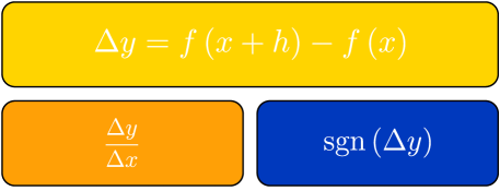
Figure 9.1: The idea behind the definition of the local trend operator is as follows. Let us observe the term: $\Delta y=f(x+\Delta x)-f(x)$. If $f$ is continuous then $\underset{\Delta x\to 0}{\lim}\Delta y=0$. Thus, we refrain from applying the limit process directly to $\Delta y$. The derivative, however, is rendered informative by comparing $\Delta y$ to $\Delta x$, via a fraction, prior to applying the limit process. The trend operator leverages less information, and quantizes $\Delta y$ via the function $\text{sgn}\left(\cdot\right)$. A function’s local trend does not reveal the information regarding its rate of change. In return, it is defined for a broad set of non-differentiable functions, as we show in the discussion below.

9.1.3 A Trends Calculation Workaround in Continuous Domains

Given this operator’s practical merit in discrete domains, we proceed with theoretical aspects in continuous domains.

Let us compare the way this operator describes local trends relative to the derivative. We define a family of monomials and attempt describing their local trend as follows: $f\left(x;a,r\right)=ax^{r}$, where $f\left(0\right)=\begin{cases}\underset{x\to 0}{\lim}f\left(x\right),&\left|\underset{x\to 0}{\lim}f\left(x\right)\right|<\infty\\ 0,&\text{otherwise.}\end{cases}$. To gain intuition, let us scrutinize the one-sided limit $\underset{\Delta x\rightarrow 0^{+}}{\lim}\text{sgn}\left(\Delta y\right)$ and compare it to the right-derivative for cherry-picked cases. Let $r\in\left\{-1,0,0.5,1,2,3\right\}$, capturing discontinuity, constancy, cusp, linearity, extremum, and inflection, respectively. We allow opposite values of $a$ to cover all types of trends. An animation illustrating the calculation of these functions’ trends via the derivative sign vs. the suggested trend operator is available in [876]. A static and partial version is available in figure 9.2.

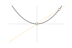
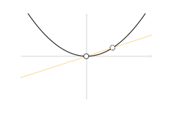
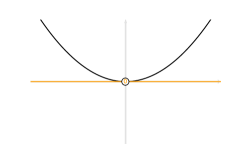
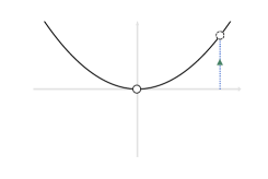
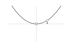
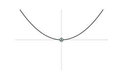
Figure 9.2: The secant line’s slope is positive throughout the finite steps of the limit process. However, the tanget’s slope (calculated at the limit) is zeroed and does not reflect the positive local trend at the local minimum. In contrast, the difference sign between the functions’ values and their value at the point remains positive at the limit.

In table 9.1, we summarize the calculations results and generalize it to all possible values of $r\in\mathbb{R}$, where $a>0$.

Scenario	$\text{sgn}\left(\lim_{x\to 0^{+}}\frac{\Delta y}{\Delta x}\right)$	$\lim_{x\to 0^{+}}\text{sgn}\left(\Delta y\right)$
$r\in\left(-\infty,0\right)\bigcup\left(0,1\right)$	$+\infty$	$1$
$r=0$	$0$	$0$
$r=1$	$1$	$1$
$r\in\left(1,\infty\right)$	$0$	$1$

Table 9.1: A summary of the trend values as calculated with the derivative sign and the suggested trend operator. Note that, except for two cases (where $k\in\left\{0,1\right\}$, accounting for constancy and linearity) where both operators yield identical results, the concise trend operator represents local trends more coherently than does the derivative sign.

As we have seen, in all these cases, $\underset{\Delta x\rightarrow 0^{+}}{\lim}\text{sgn}\left(\Delta y\right)$ reflects the way we think about the trend; that is, it always equals $a$ except for the constancy case, where it is zeroed, as expected. From table 9.1, we conclude that the derivative sign does not capture momentary trends except for $k\in\left\{0,1\right\}$.
Thus, this operator does a better job in capturing trends at critical points. Let us calculate these limits rigorously with $\epsilon-\delta$ calculus in the following discussion and establish a first result that explains why this operator outperforms the derivative sign.

9.2 Intuition

9.2.1 Why Does it Work

Let us recall Fermat’s stationary point theorem from differential Calculus.

Theorem 9.2.1 — Fermat’s stationary point theorem. 

Let $f:\left(a,b\right)\rightarrow\mathbb{R}$ be a function, and let $x\in\left(a,b\right).$ If $f$ has a local extremum at $x$ and is differentiable there then:

$$\underset{h\rightarrow 0}{\lim}\frac{f\left(x+h\right)-f\left(x\right)}{h}=0.$$

We can establish a more rigorous justification by noticing how the definition of local extrema points coalesces with that of the operator at stake. In contrast with its basic Calculus analog, the following claim provides both a sufficient and necessary condition for stationary points:

Theorem 9.2.2 — A semi-discrete Fermat’s stationary point theorem. 

Let $f:\left(a,b\right)\rightarrow\mathbb{R}$ be a function and let $x\in\left(a,b\right).$ The following condition is necessary and sufficient for $x$ to be a strict local extremum of $f$:

$$\exists\underset{h\rightarrow 0}{\lim}\text{sgn}\left[f\left(x+h\right)-f\left(x\right)\right]\neq 0.$$

The proof of this semi-discrete analogue of Fermat’s theorem immediately follows from the Cauchy limit definition.

Proof.

Without loss of generality, we will prove the theorem for maxima points. We show that the following definitions of local extrema are equivalent:

$$\begin{array}[]{ccc}&\exists\delta>0:\left|x-\bar{x}\right|<\delta\Longrightarrow f\left(x\right)>f\left(\bar{x}\right)\\ &\Updownarrow\\ &\underset{{\scriptscriptstyle h\rightarrow 0^{\pm}}}{\lim}\text{sgn}\left[f\left(x+h\right)-f\left(x\right)\right]=-1\end{array}$$

First direction. Assume $\underset{{\scriptscriptstyle h\rightarrow 0^{\pm}}}{\lim}\text{sgn}\left[f\left(x+h\right)-f\left(x\right)\right]=-1.$ Then according to Cauchy limit definition,

$$\forall\epsilon,\exists\delta:\left|x-\bar{x}\right|<\delta\Longrightarrow\left|\text{sgn}\left[f\left(\bar{x}\right)-f\left(x\right)\right]-\left(-1\right)\right|<\epsilon.$$

In particular, for $\epsilon_{0}=\frac{1}{2}$,

$$\exists\delta:\left|x-\bar{x}\right|<\delta\Longrightarrow\left|\text{sgn}\left[f\left(\bar{x}\right)-f\left(x\right)\right]+1\right|<\frac{1}{2}.$$

The only value in the sign function’s image, $\left\{0,\pm 1\right\}$, that satisfies the above inequality, is $-1$. Therefore:

$$\exists\delta:\left|x-\bar{x}\right|<\delta\Longrightarrow\text{sgn}\left[f\left(\bar{x}\right)-f\left(x\right)\right]=-1,$$

which can be written as:

$$\exists\delta:\left|x-\bar{x}\right|<\delta\Longrightarrow f\left(x\right)>f\left(\bar{x}\right).$$

Second direction. Let $\epsilon>0$. We know that there exists $\delta$ such that $\left|x-\bar{x}\right|<\delta$ implies that $f\left(x\right)>f\left(\bar{x}\right)$, which can be rewritten as

$$\text{sgn}\left[f\left(\bar{x}\right)-f\left(x\right)\right]=-1.$$

Thus $\text{sgn}\left[f\left(\bar{x}\right)-f\left(x\right)\right]-\left(-1\right)=0,$ and in particular

$$\left|\text{sgn}\left[f\left(\bar{x}\right)-f\left(x\right)\right]-\left(-1\right)\right|<\epsilon,$$

hence the limit definition holds.

∎

9.2.2 Where Does it Work

Next, let us check in which scenarios is this operator well defined. We will cherry-pick functions with different characteristics around $x=0$. For each such function, we ask which of the properties (continuity, differentiability, and the existence of the operator at stake, that is, the existence of a local trend from both sides), take place at $x=0$.

We would also like to find out which properties hold across an entire interval (for example, $[-1,1]$). To that end, we add two interval-related properties: Lebesgue and Riemann integrability. Feel free to explore these properties in 9.3.

We may extend the discussion to properties that hold in intervals almost everywhere, rather than throughout the interval. This is out of this chapter’s scope, but as an example, we will mention the function

$$f(x)=\sum\limits_{n=1}^{\infty}f_{n}(x),$$

where $f_{n}(x)=2^{-n}\phi\left(\frac{x-a_{n}}{b_{n}-a_{n}}\right),\phi$ is the Cantor-Vitali function and $\{(a_{n},b_{n}):n\in\mathbb{N}\}$ is the set of all intervals in $\left[0,1\right]$ with rational endpoints. It’s possible to show that this function has trend everywhere, it’s strictly monotonic, but its derivative is zeroed almost everywhere. In this example, the notion of instantaneous trend is coherent with the function’s monotonic behavior in the interval, in contrast with the vanishing derivative. Note that according to Baire categorization theorem, almost all the continuous functions are nowhere differentiable. Therefore, we could use an extension to the set of functions whose monotony can be analyzed concisely. Finally, we mention the function

$$g\left(x\right)=x^{1+\boldsymbol{1}_{\mathbb{Q}}}$$

defined over $\left(0,1\right)$. In its definition domain, $g$ is discontinuous everywhere, but detachable from left almost everywhere.

9.3 Definitions

9.3.1 The Instantaneous Trend of Change

Let us summarize our discussion thus far. The momentary trend, a basic analytical concept, has been embodied by the derivative sign for engineering purposes. It’s applied to constitutive numeric algorithms across AI, optimization, and other computerized applications. More often than not, it does not capture the momentary trend of change at critical points. In contrast, $\underset{\Delta x\rightarrow 0^{\pm}}{\lim}\text{sgn}\left(\Delta y\right)$ is more numerically robust, in terms of finite differences. It defines trends coherently wherever they exist, including at critical points.

Given these merits, we dedicate a definition to this operator. As it "detaches" functions, turning them into step functions with discontinuities at extrema points, let us define the one-sided detachments of a function $f$ as follows.

Definition 9.3.1 — Detachment of a real function. 

Let $f:\mathbb{R}\rightarrow\mathbb{R}$ be a function and $x\in\mathbb{R}$ a point in its definition domain. Then we define its one-sided right- and left- detachments at $x$ as follows:

$$\begin{array}[]{ccc}&f_{\pm}^{;}:\;\mathbb{R}\rightarrow\left\{-1,0,+1\right\}\\ &f_{\pm}^{;}\left(x\right)\equiv\pm\underset{{\scriptscriptstyle h\rightarrow 0^{\pm}}}{\lim}\text{sgn}\left[f\left(x+h\right)-f\left(x\right)\right].\end{array}$$

We say that a function is detachable if both those one-sided limits exist. We add the $\pm$ coefficient for consistency with the derivative sign. For convenience and brevity, from now on we denote by $f^{;}$ either one of the one-sided detachments separately ($f^{;}_{+}$ or $f^{;}_{-}$), without assuming that they necessarily agree.

Geometrically speaking, for a function’s (right-) detachment to equal $+1$, for example, its value at the point needs to strictly bound the function’s values in a right-neighborhood of $x$ from below. This is in contrast with the derivative’s sign, where we make the assumption of the existence of an ascending tangent.

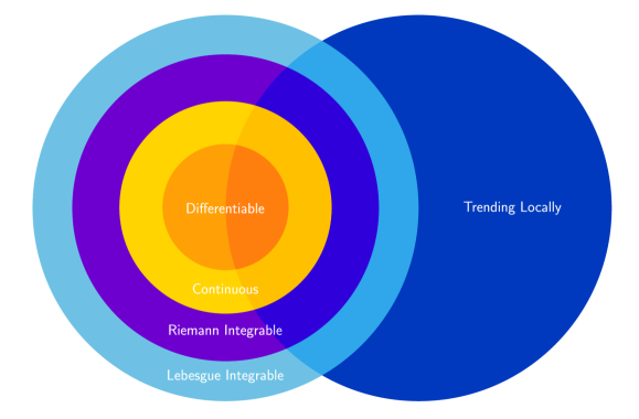
Figure 9.3: Let us illustrate the set of detachable functions in the space of real functions. Examples of functions adhering to these properties in a pointwise fashion or an interval are available in tables 9.2, 9.3, respectively.

Function	Continuous	Differentiable	Trending Locally
$f_{1}\left(x\right)=x^{2}$	V	V	V
$f_{2}\left(x\right)=\left(\frac{1}{2}-\boldsymbol{1}_{\mathbb{Q}}\right)x^{2}$	V	V
$f_{3}\left(x\right)=x^{\frac{1}{3}}$	V		V
$f_{4}\left(x\right)=\text{sgn}\left(x\right)$			V
$f_{5}\left(x\right)=\begin{cases}\sin\left(\frac{1}{x}\right),&x\neq 0\\ 0,&x=0\end{cases}$
$f_{6}\left(x\right)=x^{1+2\cdot\boldsymbol{1}_{\mathbb{Q}}}$	V		V
$f_{7}\left(x\right)=\begin{cases}\sin\left(\frac{1}{x}\right),&x\neq 0\\ 2,&x=0\end{cases}$			V
$f_{8}\left(x\right)=\begin{cases}x^{2}\sin\left(\frac{1}{x}\right),&x\neq 0\\ 0,&x=0\end{cases}$	V	V
$f_{9}\left(x\right)=\sqrt{\left|x\right|}$	V		V
$f_{10}\left(x\right)=\begin{cases}x\sin\left(\frac{1}{x}\right),&x\neq 0\\ 0,&x=0\end{cases}$	V
$f_{11}\left(x\right)=\boldsymbol{1}_{\mathbb{Z}}$			V
$f_{12}\left(x\right)=\boldsymbol{1}_{\mathbb{Q}}$ (Dirichlet)
$f_{13}\left(x\right)=\sum_{n=1}^{\infty}\left(\frac{1}{2}\right)^{n}\cos\left(3^{n}x\right)$ (Weierstrass)	V		V
$f_{14}\left(x\right)=\begin{cases}x+x\left|\sin\left(\frac{1}{x}\right)\right|,&x\neq 0\\ 0,&x=0\end{cases}$	V		V
$f_{15}\left(x\right)=\begin{cases}\frac{1}{x},&x\neq 0\\ 0,&x=0\end{cases}$			V
$f_{16}\left(x\right)=t\left(x-\sqrt{2}\right)$ (Thomae)	V
$f_{17}\left(x\right)=R\left(x\right)$ (Riemann)	V		V

Table 9.2: Relation between selected functions’ analytical properties at the point $x=0$, corresponding to figure 9.3, and some of these functions, along with their one-sided detachments, are plotted in figure 9.5.

Function	Cont.	Diff.	Trend.	Riemman	Lebesgue
$f_{1}\left(x\right)=\boldsymbol{1}_{\mathbb{Q}}$					V
$f_{2}\left(x\right)=\begin{cases}\sin\left(\frac{1}{x}\right),&x\neq 0\\ 0.5,&x=0\end{cases}$				V	V
$f_{3}\left(x\right)=\begin{cases}\sin\left(\frac{1}{x}\right),&x\neq 0\\ 0,&x=0\end{cases}$	V			V	V
$f_{4}\left(x\right)=\begin{cases}x^{2}\sin\left(\frac{1}{x}\right),&x\neq 0\\ 0,&x=0\end{cases}$	V	V		V	V
$f_{5}\left(x\right)=x$	V	V	V	V	V
$f_{6}\left(x\right)=\sqrt{\left|x\right|}$	V		V	V	V
$f_{7}\left(x\right)=\text{sgn}\left(x\right)$			V	V	V
$f_{8}\left(x\right)=\begin{cases}\frac{1}{\sqrt{\left|x\right|}},&x\neq 0\\ 0,&x=0\end{cases}$			V		V
$f_{9}\left(x\right)=\begin{cases}\frac{1}{x},&x\neq 0\\ 0,&x=0\end{cases}$			V

Table 9.3: Relation between selected functions’ analytical properties at every point of the closed intervals $\left[-1,+1\right]$, corresponding to Figure 9.3. Cont., Diff., Trend., Riemann, and Lebesgue stand for continuity, differentiability, the existence of a local trend, Riemann integrability, and Lebesgue integrability, across the interval.

9.3.2 Sign Continuity

In the discussion below we do not restrict ourselves merely to continuous functions. It turns out, that the ability to extend results to discontinuity requires to handle various cases differently. The following definitions will be useful upon classifying these cases.

For example, we may be naturally inclined to introduce product and quotient rules for the detachment operator; the following example illustrates that this may not be as straight-forward as we would imagine.

Example 9.3.1 

Let $f,g$ be functions defined at a point $x$ and in its neighborhood. If $f^{;}=g^{;}=+1$, and $f=g=0$ at a point $x$, then the detachment of the product is $\left(fg\right)^{;}\left(x\right)=+1$ as well. Following this simple scenario, one might intuitively think that the product rule for the detachment is simply $\left(fg\right)^{;}=f^{;}g^{;}$. However, upon shifting $g$ vertically downwards, that is, requiring that $g(x)<0$, we obtain a setting where $\left(fg\right)^{;}=-1$, although the detachments of $f,g$ remain as before. This means that the detachment of the product $\left(fg\right)^{;}\left(x\right)$ necessarily also depends on the sign of $f,g$ at the point of interest. Indeed, assuming $g$ is continuous, the product’s detachment in this new setting is $-1$.

However, let us recall that in Semi-discrete Calculus we are not restricted to differentiable or even continuous functions. What if $g$ is discontinuous? As long as $g$ maintains its sign in a neighborhood of the point, it is possible to show that the detachment of the product remains $-1$. But if $g$ changes its sign, meaning there is a neighborhood of $x$ where $g$ is zeroed or one where $g$ is positive, then $\left(fg\right)^{;}\left(x\right)$ can be either $0$ or $+1$, respectively. This implies that we should somehow bound the functions’ signs. It would be convenient to pay attention to the following intuitive trait of the functions $f,g$.

Definition 9.3.2 — Sign Continuity. 

Given a function $f$, we say that it is sign-continuous (s.c.) at a point $x$ if $\text{sgn}\left(f\right)$ is continuous.

Discontinuous and sign-discontinuous	Continuous and sign-discontinuous
Discontinuous and sign-continuous	Continuous and sign-continuous

Figure 9.4: Illustration of the relation between continuity and sign-continuity. Each function illustrates different constellations of these properties at $x=0$.

Definition 9.3.3 — Sign-discontinuity. 

Given a function $f$, we say that it is sign-discontinuous (s.d.) at a point $x$ if all the partial limits of $\text{sgn}\left(f\right)$ are different than its sign at $x$.

Observe that the function’s sign-continuity at a point may be determined given its sign and detachment. For example, if $f^{;}\left(x\right)=0$ or $\left(ff^{;}\right)\left(x\right)>0$, then $f$ is sign-continuous. This observation suggests the following definition.

Definition 9.3.4 — Inherent Sign-continuity (discontinuity). 

We say that $f$ is inherently sign-continuous (sign-discontinuous), abbreviated by i.s.c. (i.s.d.) at a point $x$ if the knowledge of its sign and detachment at the point alone determine its sign-continuity (sign-discontinuity).

For convenience, we limit the following discussion to sign-continuous or sign-discontinuous functions.

Definition 9.3.5 — Sign-consistency. 

We call a function that is either sign-continuous or sign-discontinuous "sign-consistent".

9.4 Semi-discrete Analogues to Calculus Theorems

Equipped with a concise definition of the instantaneous trend of change, we may formulate analogs to Calculus theorems with the following trade-off. Those simple corollaries inform us of the function’s trend rather than its rate. In return, they hold for a broad set of detachable and non-differentiable functions.

$f_{1}\left(x\right)=x^{2}$	$f_{2}\left(x\right)=\left(\frac{1}{2}-\boldsymbol{1}_{\mathbb{Q}}\right)x^{2}$	$f_{3}\left(x\right)=x^{\frac{1}{3}}$
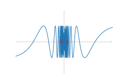
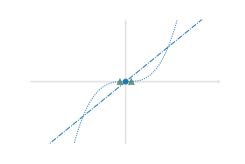
$f_{4}\left(x\right)=\text{sgn}\left(x\right)$	$f_{5}\left(x\right)=\begin{cases}\sin\left(\frac{1}{x}\right),&x\neq 0\\ 0,&x=0\end{cases}$	$f_{6}\left(x\right)=x^{1+2\cdot\boldsymbol{1}_{\mathbb{Q}}}$
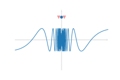
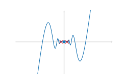
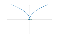
$f_{7}\left(x\right)=\begin{cases}\sin\left(\frac{1}{x}\right),&x\neq 0\\ 2,&x=0\end{cases}$	$f_{8}\left(x\right)=\begin{cases}x^{2}\sin\left(\frac{1}{x}\right),&x\neq 0\\ 0,&x=0\end{cases}$	$f_{9}\left(x\right)=\sqrt{\left|x\right|}$
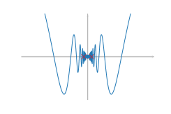
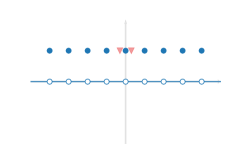
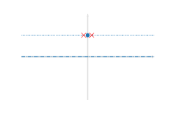
$f_{10}\left(x\right)=\begin{cases}x\sin\left(\frac{1}{x}\right),&x\neq 0\\ 0,&x=0\end{cases}$	$f_{11}\left(x\right)=\boldsymbol{1}_{\mathbb{Z}}$	$f_{12}\left(x\right)=\boldsymbol{1}_{\mathbb{Q}}$
$f_{13}\left(x\right)=\sum_{n=1}^{\infty}\left(\frac{1}{2}\right)^{n}\cos\left(3^{n}x\right)$	$f_{14}\left(x\right)=\begin{cases}x+x\left|\sin\left(\frac{1}{x}\right)\right|,&x\neq 0\\ 0,&x=0\end{cases}$	$f_{15}\left(x\right)=\begin{cases}\frac{1}{x},&x\neq 0\\ 0,&x=0\end{cases}$

Figure 9.5: The one-sided detachments of selected functions at $x=0$, denoted with upper or lower carets next to $f\left(0\right)$ if the detachment exists. Non detachable functions there are annotated with "X". Other properties of these functions are detailed in table 9.2.

9.4.1 Simple Algebraic Properties

Claim 9.4.1 

A semi-discrete constant multiple rule. If $f$ is detachable at $x$, and $c\in\mathbb{R}$ is a constant, then $cf$ is also detachable and the following holds there:

$$\left(cf\right)^{;}=\text{sgn}\left(cf^{;}\right).$$

Proof.

$$\begin{aligned} \left(cf\right)_{\pm}^{;}&=\pm\underset{t\rightarrow x^{\pm}}{\lim}\text{sgn}\left[\left(cf\right)\left(x+h\right)-\left(cf\right)\left(x\right)\right]\\ &=\pm\underset{t\rightarrow x^{\pm}}{\lim}\text{sgn}\left(c\right)\text{sgn}\left[f\left(x+h\right)-f\left(x\right)\right]\\ &=\text{sgn}\left(c\right)f_{\pm}^{;}=\text{sgn}\left[cf_{\pm}^{;}\right].\end{aligned}$$ (9.4)

∎

Claim 9.4.2 

Semi-discrete sum and difference Rules. If $f$ and $g$ are detachable at $x$ and $\left(f^{;}g^{;}\right)\left(x\right)\in\left\{0,\pm 1\right\}$ (the plus or minus signs are for the sum and difference rules, respectively), then the following holds at $x$:

$$\left(f\pm g\right)^{;}=\text{sgn}\left(f^{;}\pm g^{;}\right).$$

Proof.

Without loss of generality, let us focus on right-detachments. We will show that if $f^{;}_{+}\left(x\right)=g^{;}_{+}\left(x\right)$ then $\left(f+g\right)^{;}_{+}\left(x\right)=+1$, and the rest of the cases are proved similarly.

There is a right-neighborhood bounded by $\delta_{f}$ where:

$$0<\bar{x}-x<\delta_{f}\Longrightarrow\text{sgn}\left[f\left(\bar{x}\right)-f\left(x\right)\right]=+1\Longrightarrow f\left(\bar{x}\right)>f\left(x\right).$$

Similarly there exists a right-neighborhood bounded by $\delta_{g}$ where:

$$0<\bar{x}-x<\delta_{g}\Longrightarrow g\left(\bar{x}\right)>g\left(x\right).$$

Therefore there is a right-neighborhood bounded by $\delta_{f+g}\equiv\min\left\{\delta_{f},\delta_{g}\right\}$ where:

$$0<\bar{x}-x<\delta_{f+g}:\,\,\text{sgn}\left[\left(f+g\right)\left(\bar{x}\right)-\left(f+g\right)\left(x\right)\right]=+1,$$

hence

$$\underset{\bar{x}\rightarrow x^{+}}{\lim}\text{sgn}\left[\left(f+g\right)\left(\bar{x}\right)-\left(f+g\right)\left(x\right)\right]=+1.$$

∎

Claim 9.4.3 

If $f$, $g$ and $f+g$ are detachable at $x$, and the one-sided detachments of $f$ and $g$ aren’t both zeroed, then the following holds at $x$:

$$f^{;}g^{;}=\left(f+g\right)^{;}\left(f^{;}+g^{;}\right)-1.$$

Proof.

It is possible to show by separating to cases that for $A,B$ not both zero:

$$\text{sgn}\left(A\right)\text{sgn}\left(B\right)=\text{sgn}\left(A+B\right)\left[\text{sgn}\left(A\right)+\text{sgn}\left(B\right)\right]-1.$$

The result is obtained by taking $A=f\left(x+h\right)-f\left(x\right)$ and $B=g\left(x+h\right)-g\left(x\right)$, followed by applying the one-sided limit process to both sides. ∎

This sum rule holds only for functions whose detachments are not additive inverses. We will handle those cases, assuming differentiability, later on with Taylor series.

9.4.2 Product and Quotient Rules

In the process of formulating the product rule, we repeatedly conduct analyses similar to the above, with different combinations of $f^{;},g^{;}$, their signs, and assumptions on their sign-continuity or lack of.

The following link includes a simulation code for the creation of the data required to extract those rules. The final results obtained from the simulation are also available here.

In each of these cases, we conduct an $\epsilon-\delta$ analysis and prove that the product’s detachment equals a value, in case it’s indeed determined.

Recall that the product rule for derivatives dictates the following combination of the original functions’ derivatives:

$$\left(fg\right)^{\prime}=f^{\prime}g+fg^{\prime}.$$

Evidently, the results we gather regarding the detachments product follow a similar rule in part of the cases and follow another intuitive formula in others. Recall that the following product and quotient rules hold for detachable, not necessarily continuous functions.

Theorem 9.4.1 — A semi-discrete product rule. 

Let $f$ and $g$ be detachable and sign-consistent at $x$. If one of the following holds there:

1. $ff^{;}gg^{;}\geq 0$, where $f$ or $g$ is s.c., or

2. $f=g=0$ $ff^{;}gg^{;}<0$, where $f$ or $g$ is s.d.

Then $fg$ is detachable there, and:

$$\left(fg\right)^{;}=\begin{cases}\text{sgn}\left[f^{;}\text{sgn}\left(g\right)+g^{;}\text{sgn}\left(f\right)\right],&ff^{;}gg^{;}\geq 0\text{, and }f\text{ or }g\text{ is s.c.}\\ f^{;}g^{;},&\text{else}\text{.}\end{cases}$$

Proof.

For brevity, we will refer to the terms $\text{sgn}\left[f^{;}\text{sgn}\left(g\right)+g^{;}\text{sgn}\left(f\right)\right]$ and $f^{;}g^{;}$ from the theorem statement as the first and second formulas, respectively.

Let us distinguish between the following cases, according to the pointwise signs of $f,g$ and their detachments (the vector $\left(f^{;},\text{sgn}\left(f\right),g^{;},\text{sgn}\left(g\right)\right)\in\left\{\pm 1,0\right\}^{4}$), and their inherent sign-continuity or lack of.

1. Assume $ff^{;}gg^{;}>0$. There are 8 such combinations of $\left(f^{;},\text{sgn}\left(f\right),g^{;},\text{sgn}\left(g\right)\right)$:

   • Assume that either $f$ or $g$ is inherently sign-continuous. There are 4 such cases, in which both $f,g$ adhere to the inherent sign-continuity property. Without loss of generality assume that $f^{;}=g^{;}=\text{sgn}\left(f\right)=\text{sgn}\left(g\right)=+1$. Then:

     $$\begin{cases}\exists\delta_{f}:&\forall\bar{x}\in B_{\delta_{f}}\left(x\right):f\left(\bar{x}\right)>f\left(x\right)>0\\ \exists\delta_{g}:&\forall\bar{x}\in B_{\delta_{g}}\left(x\right):g\left(\bar{x}\right)>g\left(x\right)>0\end{cases}$$

     hence for $\delta_{fg}\equiv\min\left\{\delta_{f},\delta_{g}\right\}$ it holds that:

     $$\forall\bar{x}\in B_{\delta_{fg}}\left(x\right):\left(fg\right)\left(\bar{x}\right)=f\left(\bar{x}\right)g\left(\bar{x}\right)>f\left(x\right)g\left(x\right)=\left(fg\right)\left(x\right),$$

     and $\left(fg\right)^{;}\left(x\right)=+1=\text{sgn}\left[\left(+1\right)\cdot\left(+1\right)+\left(+1\right)\cdot\left(+1\right)\right]$, in accordance with the second formula.

   • Assume that neither $f$ nor $g$ is inherently sign-continuous. There are 4 such cases. Without loss of generality assume that $f^{;}=g^{;}=+1$ and $f,g<0$. Then:

     $$\begin{cases}\exists\delta_{f}^{\left(1\right)}:&\forall\bar{x}\in B_{\delta_{f}^{\left(1\right)}}\left(x\right):f\left(\bar{x}\right)>f\left(x\right)\\ \exists\delta_{g}:&\forall\bar{x}\in B_{\delta_{g}}\left(x\right):g\left(\bar{x}\right)>g\left(x\right)\\ &f\left(x\right)<0\\ &g\left(x\right)<0\end{cases}$$

     The continuity of $\text{sgn}\left(f\right)$ cannot be inferred directly from the definition of the detachment and its value’s sign. Therefore, we will assume that $f$ is sign-continuous explicitly: $\exists\delta_{f}^{\left(2\right)}:\forall\bar{x}\in B_{\delta_{f}^{\left(2\right)}}\left(x\right):f\left(\bar{x}\right)<0,$ hence for $\delta_{fg}\equiv\min\left\{\delta_{f^{\left(1\right)}},\delta_{f^{\left(2\right)}},\delta_{g}\right\}$ it holds that:

     $$\forall\bar{x}\in B_{\delta_{fg}}\left(x\right):\left(fg\right)\left(\bar{x}\right)=f\left(\bar{x}\right)g\left(\bar{x}\right)<f\left(\bar{x}\right)g\left(x\right)<f\left(x\right)g\left(x\right)=\left(fg\right)\left(x\right),$$

     and $\left(fg\right)^{;}\left(x\right)=-1=\text{sgn}\left[\left(+1\right)\cdot\left(-1\right)+\left(+1\right)\cdot\left(-1\right)\right]$, in accordance with the second formula.

2. Assume $ff^{;}gg^{;}=0$. There are 65 such combinations of $\left(f^{;},\text{sgn}\left(f\right),g^{;},\text{sgn}\left(g\right)\right)$:

   • Assume that $f$ or $g$ is sign-continuous. There are 61 such combinations: Assume that one of $f,g$ is inherently sign-continuous and the other is inherently sign-discontinuous. There are 20 such combinations of $\left(f^{;},\text{sgn}\left(f\right),g^{;},\text{sgn}\left(g\right)\right)$. Without loss of generality, assume that $f^{;}=g^{;}=-1,f<0$ and $g=0$, where $f$ is inherently sign-continuous and $g$ is inherently sign-discontinuous. Then:

     $$\begin{cases}\exists\delta_{f}:&\forall\bar{x}\in B_{\delta_{f}}\left(x\right):f\left(\bar{x}\right)<f\left(x\right)<0\\ \exists\delta_{g}:&\forall\bar{x}\in B_{\delta_{g}}\left(x\right):g\left(\bar{x}\right)<g\left(x\right)=0\end{cases}$$

     hence for $\delta_{fg}\equiv\min\left\{\delta_{f},\delta_{g}\right\}$ it holds that:

     $$\forall\bar{x}\in B_{\delta_{fg}}\left(x\right):\left(fg\right)\left(\bar{x}\right)=f\left(\bar{x}\right)g\left(\bar{x}\right)>0=\left(fg\right)\left(x\right),$$

     and $\left(fg\right)^{;}\left(x\right)=+1=\text{sgn}\left[\left(-1\right)\cdot 0+\left(-1\right)\cdot\left(-1\right)\right]$, in accordance with the second formula.

   • Assume that one of $f,g$ is inherently sign-continuous and the other is neither inherently sign-continuous nor inherently sign-discontinuous. There are 12 such combinations of $\left(f^{;},\text{sgn}\left(f\right),g^{;},\text{sgn}\left(g\right)\right)$. Without loss of generality, assume that $f^{;}=0,g^{;}=-1,f<0$ and $g>0$, where $f$ is inherently sign-continuous. Then:

     $$\begin{cases}\exists\delta_{f}:&\forall\bar{x}\in B_{\delta_{f}}\left(x\right):f\left(\bar{x}\right)=f\left(x\right)<0\\ \exists\delta_{g}:&\forall\bar{x}\in B_{\delta_{g}}\left(x\right):g\left(\bar{x}\right)<g\left(x\right)\\ &g\left(x\right)>0\end{cases}$$

     hence for $\delta_{fg}\equiv\min\left\{\delta_{f},\delta_{g}\right\}$ it holds that:

     $$\forall\bar{x}\in B_{\delta_{fg}}\left(x\right):\left(fg\right)\left(\bar{x}\right)=f\left(\bar{x}\right)g\left(\bar{x}\right)>f\left(x\right)g\left(x\right)=\left(fg\right)\left(x\right),$$

     and $\left(fg\right)^{;}\left(x\right)=+1=\text{sgn}\left[\left(0\right)\cdot\left(+1\right)+\left(-1\right)\cdot\left(-1\right)\right],$ in accordance with the second formula.

   • Assume that one of $f,g$ is inherently sign-discontinuous and the other is neither inherently sign-continuous nor inherently sign-discontinuous. There are 8 such combinations of $\left(f^{;},\text{sgn}\left(f\right),g^{;},\text{sgn}\left(g\right)\right)$. Without loss of generality, assume that $f^{;}=g^{;}=-1,f>0$ and $g=0$, where $g$ is inherently sign-discontinuous and $f$ is neither inherently sign-continuous nor sign-discontinuous. Then:

     $$\begin{cases}\exists\delta_{f^{\left(1\right)}}:&\forall\bar{x}\in B_{\delta_{f}^{\left(1\right)}}\left(x\right):f\left(\bar{x}\right)<f\left(x\right)<0\\ \exists\delta_{g}:&\forall\bar{x}\in B_{\delta_{g}}\left(x\right):g\left(\bar{x}\right)<g\left(x\right)=0\end{cases}$$

     Let us assume the continuity of $f$ at $x$ explicitly: $\exists\delta_{f^{\left(2\right)}}:\forall\bar{x}\in B_{\delta_{f}^{\left(2\right)}}\left(x\right):f\left(\bar{x}\right)<0,$ hence for $\delta_{fg}\equiv\min\left\{\delta_{f}^{\left(1\right)},\delta_{f}^{\left(2\right)},\delta_{g}\right\}$ it holds that:

     $$\forall\bar{x}\in B_{\delta_{fg}}\left(x\right):\left(fg\right)\left(\bar{x}\right)=f\left(\bar{x}\right)g\left(\bar{x}\right)<0=\left(fg\right)\left(x\right),$$

     and $\left(fg\right)^{;}\left(x\right)=-1=\text{sgn}\left[\left(-1\right)\cdot 0+\left(-1\right)\cdot\left(+1\right)\right]$, in accordance with the second formula.

   • Assume that both $f,g$ are inherently sign-continuous. There are 21 such combinations of $\left(f^{;},\text{sgn}\left(f\right),g^{;},\text{sgn}\left(g\right)\right)$. Without loss of generality, assume that $f^{;}=g^{;}=0,f<0$ and $g<0$, where $f,g$ are both inherently sign-continuous. Then:

     $$\begin{cases}\exists\delta_{f}:&\forall\bar{x}\in B_{\delta_{f}}\left(x\right):f\left(\bar{x}\right)=f\left(x\right)<0\\ \exists\delta_{g}:&\forall\bar{x}\in B_{\delta_{g}}\left(x\right):g\left(\bar{x}\right)<g\left(x\right)<0\end{cases}$$

     hence for $\delta_{fg}\equiv\min\left\{\delta_{f},\delta_{g}\right\}$ it holds that:

     $$\forall\bar{x}\in B_{\delta_{fg}}\left(x\right):\left(fg\right)\left(\bar{x}\right)=f\left(\bar{x}\right)g\left(\bar{x}\right)>f\left(x\right)g\left(x\right)=\left(fg\right)\left(x\right),$$

     and $\left(fg\right)^{;}\left(x\right)=0=\text{sgn}\left[\left(0\right)\cdot\left(-1\right)+\left(0\right)\cdot\left(-1\right)\right]$, in accordance with the second formula.

   • Assume that $f=g=0$. There are 4 such combinations of $\left(f^{;},\text{sgn}\left(f\right),g^{;},\text{sgn}\left(g\right)\right)$. In these cases, both $f,g$ are inherently sign-discontinuous. Without loss of generality, assume that $f^{;}=g^{;}=1,f=g=0$, where $f,g$ are both inherently sign-discontinuous. Then:

     $$\begin{cases}\exists\delta_{f}:&\forall\bar{x}\in B_{\delta_{f}}\left(x\right):f\left(\bar{x}\right)<f\left(x\right)=0\\ \exists\delta_{g}:&\forall\bar{x}\in B_{\delta_{g}}\left(x\right):g\left(\bar{x}\right)<g\left(x\right)=0\end{cases}$$

     hence for $\delta_{fg}\equiv\min\left\{\delta_{f},\delta_{g}\right\}$ it holds that:

     $$\forall\bar{x}\in B_{\delta_{fg}}\left(x\right):\left(fg\right)\left(\bar{x}\right)=f\left(\bar{x}\right)g\left(\bar{x}\right)>0=f\left(x\right)g\left(x\right)=\left(fg\right)\left(x\right),$$

     and $\left(fg\right)^{;}\left(x\right)=+1=\left(+1\right)\cdot\left(+1\right)$, in accordance with the first formula.

3. Assume $ff^{;}gg^{;}<0$. There are 8 such combinations of $\left(f^{;},\text{sgn}\left(f\right),g^{;},\text{sgn}\left(g\right)\right)$. For each combination it holds that $ff^{;}>0$ or $gg^{;}>0$, hence either $f$ or $g$ is inherently sign-continuous. Without loss of generality assume that $f^{;}=+1,f>0,g^{;}=-1$ and $g>0$. Then:

   $$\begin{cases}\exists\delta_{f}:&\forall\bar{x}\in B_{\delta_{f}^{\left(1\right)}}\left(x\right):f\left(\bar{x}\right)>f\left(x\right)>0\\ \exists\delta_{g}^{\left(1\right)}:&\forall\bar{x}\in B_{\delta_{g}}\left(x\right):g\left(\bar{x}\right)<g\left(x\right)\\ &g\left(x\right)>0\end{cases}$$

   The continuity of $\text{sgn}\left(f\right)$ can be inferred directly from the definition of the detachment and its value’s sign. However, $g$ is neither inherently sign-continuous nor inherently sign-discontinuous. Thus we will assume that $g$ is sign-discontinuous explicitly:

   $$\exists\delta_{g}^{\left(2\right)}:\forall\bar{x}\in B_{\delta_{g}^{\left(2\right)}}\left(x\right):g\left(\bar{x}\right)\leq 0,$$

   hence for $\delta_{fg}\equiv\min\left\{\delta_{f},\delta_{g^{\left(1\right)}},\delta_{g^{\left(2\right)}}\right\}$ it holds that:

   $$\forall\bar{x}\in B_{\delta_{fg}}\left(x\right):\left(fg\right)\left(\bar{x}\right)=f\left(\bar{x}\right)g\left(\bar{x}\right)\leq 0<f\left(x\right)g\left(x\right)=\left(fg\right)\left(x\right),$$

   and $\left(fg\right)^{;}\left(x\right)=-1=\left(+1\right)\cdot\left(-1\right)$, in accordance with the first formula.

∎

Similarly to the product rule for detachment, the following quotient rule also incorporates a term that looks familiar from the nominator in its derivative counterpart, $f^{\prime}g-gf^{\prime}$.

Theorem 9.4.2 — A semi-discrete quotient rule. 

Let $f$ and $g$ be detachable and sign-consistent at $x$, where $g\neq 0$ across their definition domain. Assume that $f,g$ are either s.c. or s.d. If one of the following holds at:

1. $ff^{;}gg^{;}\leq 0$, where $f$ or $g$ is s.c., or $f=0$

2. $ff^{;}gg^{;}>0$, where only one of $f,g$ is s.c.

Then $\frac{f}{g}$ is detachable, and:

$$\left(\frac{f}{g}\right)^{;}=\begin{cases}\text{sgn}\left[f^{;}\text{sgn}\left(g\right)-g^{;}\text{sgn}\left(f\right)\right],&g\text{ is i.s.c., or }f\text{ and }g\text{ are s.c.},\text{or }f=0\text{ and }f\text{ or }g\text{ is s.c.}\\ \text{sgn}\left[f^{;}\text{sgn}\left(g\right)+g^{;}\text{sgn}\left(f\right)\right],&\text{else if }ff^{;}gg^{;}\geq 0\text{, and }f\text{ or }g\text{ is s.c.}\\ f^{;}g^{;},&\text{else.}\end{cases}$$

Proof.

For brevity, we will refer to the terms $\text{sgn}\left[f^{;}\text{sgn}\left(g\right)-g^{;}\text{sgn}\left(f\right)\right]$, $\text{sgn}\left[f^{;}\text{sgn}\left(g\right)+g^{;}\text{sgn}\left(f\right)\right]$ and $f^{;}g^{;}$ from the theorem statement as the first, second and third formulas and conditions, respectively.

We prove the claim by separating to cases. We will suggest a slightly shorter analysis with respect to the proof of the product rule, as the ideas are similar. We will survey a handful of representative cases. The rest of them are shown to hold analogously.

1. Assume that $g$ is i.s.c. Without lose of generality, assume $f^{;}=g^{;}=-1,f>0$ and $g<0$. There are two cases: either $f$ is s.d., or it is s.c.

   • Assuming $f$ is s.d., then:

     $$\begin{cases}\exists\delta_{f}^{\left(1\right)}:&\forall\bar{x}\in B_{\delta_{f}^{\left(1\right)}}\left(x\right):f\left(\bar{x}\right)<f\left(x\right)\\ \exists\delta_{f}^{\left(2\right)}:&\forall\bar{x}\in B_{\delta_{f}^{\left(2\right)}}\left(x\right):f\left(\bar{x}\right)\leq 0\\ \exists\delta_{g}:&\forall\bar{x}\in B_{\delta_{g}}\left(x\right):g\left(\bar{x}\right)<g\left(x\right)\\ &f\left(x\right)>0\\ &g\left(x\right)<0,\end{cases}$$

     hence for $\delta_{f/g}\equiv\min\left\{\delta_{f}^{\left(1\right)},\delta_{f}^{\left(2\right)},\delta_{g}\right\}$ it holds that:

     $$\forall\bar{x}\in B_{\delta_{f/g}}\left(x\right):\frac{f}{g}\left(\bar{x}\right)\in\left\{0,+1\right\},$$

     however $\frac{f}{g}\left(x\right)<0$, therefore $\text{sgn}\left[\frac{f}{g}\left(\bar{x}\right)-\frac{f}{g}\left(x\right)\right]=+1$ in a neighborhood of $x$. Thus

     $$\left(\frac{f}{g}\right)^{;}\left(x\right)=+1=\text{sgn}\left[\left(-1\right)\cdot\left(-1\right)-\left(-1\right)\cdot\left(+1\right)\right]$$

     , in accordance with the first formula.

   • Assuming $f$ is s.c. while maintaining the conditions in the previous example, we have:

     $$\exists\tilde{\delta}_{f}^{\left(2\right)}:\forall\bar{x}\in B_{\tilde{\delta}_{f}^{\left(2\right)}}\left(x\right):f\left(\bar{x}\right)>0,$$

     hence for $\tilde{\delta}{}_{f/g}\equiv\min\left\{\delta_{f}^{\left(1\right)},\tilde{\delta}_{f}^{\left(2\right)},\delta_{g}\right\}$ it holds that:

     $$\forall\bar{x}\in B_{\delta_{f/g}}\left(\bar{x}\right):\left|\frac{f}{g}\left(\bar{x}\right)\right|<\left|\frac{f}{g}\left(x\right)\right|,$$

     and since $\frac{f}{g}\left(\bar{x}\right),\frac{f}{g}\left(x\right)$ are both negative then $\frac{f}{g}\left(\bar{x}\right)>\frac{f}{g}\left(x\right)$ in that neighborhood of $x$, and again $\left(\frac{f}{g}\right)^{;}\left(x\right)=+1$.

2. Assume that $f,g$ are both s.c. Without lose of generality, assume $f^{;}=g^{;}=-1,f<0$ and $g>0$. Then $f$ is i.s.c., and we will impose the assumption that $g$ is s.c. Then:

   $$\begin{cases}\exists\delta_{f}:&\forall\bar{x}\in B_{\delta_{f}}\left(x\right):f\left(\bar{x}\right)<f\left(x\right)\\ \exists\delta_{g}^{\left(1\right)}:&\forall\bar{x}\in B_{\delta_{g}^{\left(1\right)}}\left(x\right):g\left(\bar{x}\right)\leq g\left(x\right)\\ \exists\delta_{g}^{\left(2\right)}:&\forall\bar{x}\in B_{\delta_{g}^{\left(2\right)}}\left(x\right):g\left(\bar{x}\right)>0\\ &f\left(x\right)>0\\ &g\left(x\right)<0,\end{cases}$$

   hence for $\delta_{f/g}\equiv\min\left\{\delta_{f},\delta_{g}^{\left(1\right)},\delta_{g}^{\left(2\right)}\right\}$ it holds that:

   $$\forall\bar{x}\in B_{\delta_{f/g}}\left(x\right):\left|\frac{f}{g}\left(\bar{x}\right)\right|>\left|\frac{f}{g}\left(x\right)\right|,$$

   and since $\frac{f}{g}\left(x\right),\frac{f}{g}\left(\bar{x}\right)$ are both negative, then $\frac{f}{g}\left(\bar{x}\right)<\frac{f}{g}\left(x\right)$ in that neighborhood of $x$. Thus $\left(\frac{f}{g}\right)^{;}\left(x\right)=-1=\text{sgn}\left[\left(-1\right)\cdot\left(+1\right)-\left(-1\right)\cdot\left(-1\right)\right]$, in accordance with the first formula.

3. Assume that the second conditions hold, that is, the conditions of the first formula do not hold, while $ff^{;}gg^{;}\geq 0$ and $f$ or $g$ is s.c. There are two slightly different families of cases, where $ff^{;}gg^{;}$ is either zeroed or positive.

   1. Assume first that $ff^{;}gg^{;}>0$. Without lose of generality, let $f^{;}=g^{;}=-1,f>0$ and $g>0$. Assume that $f$ is s.c. Then we can assume that $g$ is not s.c., because otherwise the first condition would hold. Then:

      $$\begin{cases}\exists\delta_{f}^{\left(1\right)}:&\forall\bar{x}\in B_{\delta_{f}^{\left(1\right)}}\left(x\right):f\left(\bar{x}\right)<f\left(x\right)\\ \exists\delta_{f}^{\left(2\right)}:&\forall\bar{x}\in B_{\delta_{f}^{\left(2\right)}}\left(x\right):f\left(\bar{x}\right)>0\\ \exists\delta_{g}^{\left(1\right)}:&\forall\bar{x}\in B_{\delta_{g}^{\left(1\right)}}\left(x\right):g\left(\bar{x}\right)<g\left(x\right)\\ \exists\delta_{g}^{\left(2\right)}:&\forall\bar{x}\in B_{\delta_{g}^{\left(2\right)}}\left(x\right):g\left(\bar{x}\right)<0\\ &f\left(x\right)>0\\ &g\left(x\right)>0,\end{cases}$$

      hence for $\delta_{f/g}\equiv\min\left\{\delta_{f}^{\left(1\right)},\delta_{f}^{\left(2\right)},\delta_{g}^{\left(1\right)},\delta_{g}^{\left(2\right)}\right\}$ it holds that:

      $$\forall\bar{x}\in B_{\delta_{f/g}}\left(x\right):\frac{f}{g}\left(\bar{x}\right)<0,$$

      and since $\frac{f}{g}\left(x\right)>0,$ then $\frac{f}{g}\left(\bar{x}\right)<\frac{f}{g}\left(x\right)$ in that neighborhood of $x$. Thus $\left(\frac{f}{g}\right)^{;}\left(x\right)=-1=\text{sgn}\left[\left(-1\right)\cdot\left(+1\right)+\left(-1\right)\cdot\left(+1\right)\right]=-1$, in accordance with the second formula.

   2. Assume that $ff^{;}gg^{;}=0$. Without lose of generality, let $f^{;}=g^{;}=-1,f=0$ and $g>0$. Since $f$ is i.s.d. we will assume that $g$ is s.c. Then:

      $$\begin{cases}\exists\delta_{f}:&\forall\bar{x}\in B_{\delta_{f}}\left(x\right):f\left(\bar{x}\right)<f\left(x\right)\\ \exists\delta_{g}^{\left(1\right)}:&\forall\bar{x}\in B_{\delta_{g}^{\left(1\right)}}\left(x\right):g\left(\bar{x}\right)<g\left(x\right)\\ \exists\delta_{g}^{\left(2\right)}:&\forall\bar{x}\in B_{\delta_{g}^{\left(2\right)}}\left(x\right):g\left(\bar{x}\right)>0\\ &f\left(x\right)=0\\ &g\left(x\right)>0,\end{cases}$$

      hence for $\delta_{f/g}\equiv\min\left\{\delta_{f},\delta_{g}^{\left(1\right)},\delta_{g}^{\left(2\right)}\right\}$ it holds that:

      $$\forall\bar{x}\in B_{\delta_{f/g}}\left(x\right):\frac{f}{g}\left(\bar{x}\right)>0,$$

      and since $\frac{f}{g}\left(x\right)>0$, then $\frac{f}{g}\left(\bar{x}\right)<\frac{f}{g}\left(x\right)$ in that neighborhood of $x$. Thus $\left(\frac{f}{g}\right)^{;}\left(x\right)=-1=\text{sgn}\left[\left(-1\right)\cdot\left(+1\right)+\left(-1\right)\cdot 0\right]$, in accordance with the second formula.

4. Assume that the third condition holds. There are two slightly different cases, where $f$ is either zeroed or not.

   • First assume that $f\left(x\right)=0$. Without lose of generality, let $f^{;}=g^{;}=-1$, and $g>0$. We can assume that $g$ is s.d., because otherwise the first formula would hold. Then:

     $$\begin{cases}\exists\delta_{f}^{\left(1\right)}:&\forall\bar{x}\in B_{\delta_{f}^{\left(1\right)}}\left(x\right):f\left(\bar{x}\right)<f\left(x\right)\\ \exists\delta_{f}^{\left(2\right)}:&\forall\bar{x}\in B_{\delta_{f}^{\left(2\right)}}\left(x\right):f\left(\bar{x}\right)>0\\ \exists\delta_{g}^{\left(1\right)}:&\forall\bar{x}\in B_{\delta_{g}^{\left(1\right)}}\left(x\right):g\left(\bar{x}\right)<g\left(x\right)\\ \exists\delta_{g}^{\left(2\right)}:&\forall\bar{x}\in B_{\delta_{g}^{\left(2\right)}}\left(x\right):g\left(\bar{x}\right)<0\\ &f\left(x\right)=0\\ &g\left(x\right)>0,\end{cases}$$

     hence for $\delta_{f/g}\equiv\min\left\{\delta_{f}^{\left(1\right)},\delta_{f}^{\left(2\right)},\delta_{g}^{\left(1\right)},\delta_{g}^{\left(2\right)}\right\}$ it holds that:

     $$\forall\bar{x}\in B_{\delta_{f/g}}\left(x\right):\frac{f}{g}\left(\bar{x}\right)>0,$$

     and since $\frac{f}{g}\left(x\right)>0,$then $\frac{f}{g}\left(\bar{x}\right)>\frac{f}{g}\left(x\right)$ in that neighborhood of $x$. Thus $\left(\frac{f}{g}\right)^{;}\left(x\right)=+1=\left(-1\right)\cdot\left(-1\right)$, in accordance with the third formula.

   • Assume that $f\left(x\right)\neq 0$. Without lose of generality, let $f^{;}=g^{;}=-1,f<0$ and $g>0$. We can assume that $g$ is s.d., because $f$ is i.s.c. and if $g$ was also s.c. then the first formula would hold. Then:

     $$\begin{cases}\exists\delta_{f}:&\forall\bar{x}\in B_{\delta_{f}}\left(x\right):f\left(\bar{x}\right)<f\left(x\right)\\ \exists\delta_{g}^{\left(1\right)}:&\forall\bar{x}\in B_{\delta_{g}^{\left(1\right)}}\left(x\right):g\left(\bar{x}\right)<g\left(x\right)\\ \exists\delta_{g}^{\left(2\right)}:&\forall\bar{x}\in B_{\delta_{g}^{\left(2\right)}}\left(x\right):g\left(\bar{x}\right)<0\\ &f\left(x\right)<0\\ &g\left(x\right)>0,\end{cases}$$

     hence for $\delta_{f/g}\equiv\min\left\{\delta_{f},\delta_{g}^{\left(1\right)},\delta_{g}^{\left(2\right)}\right\}$ it holds that:

     $$\forall\bar{x}\in B_{\delta_{f/g}}\left(x\right):\frac{f}{g}\left(\bar{x}\right)>0,$$

     and since $\frac{f}{g}\left(x\right)<0,$ then $\frac{f}{g}\left(\bar{x}\right)>\frac{f}{g}\left(x\right)$ in that neighborhood of $x$. Thus $\left(\frac{f}{g}\right)^{;}\left(x\right)=+1=\left(-1\right)\cdot\left(-1\right)$, in accordance with the third formula.

∎

In the quotient rule, if $f,g$ are both continuous then, because $g\neq 0$, $g$ has to be s.c. If $f$ is also s.c. then the first formula holds according to its second sub-condition. If $f$ is not s.c., then from its continuity, $f=0$ and the first formula holds according to its third sub-condition. Thus, the first formula holds for all the pairs of continuous functions subject to the proposition statement. However, in the product rule, the first formula does not hold for some continuous functions. For example, consider $f=g=x$ at $x=0$. Since both $f$ and $g$ are s.d., their product’s detachment follows the second formula instead. Upon formulating the aforementioned rules, there are other ways to bound the signs of the functions $f,g$ rather than inquiring about their sign continuity. For example, we could offer a precise bound on the signs of $f,g$ in a given neighborhood of $x$. A product rule constructed based on these traits holds in more cases than do claims 4 and 5. However, for consistency with Differential Calculus, I preferred to introduce in this chapter the intuitive trait of sign-continuity. This property corresponds with the traditional requirement of differentiability and continuity, and, as such, the first-time reader may feel slightly more comfortable with it. We define sign-discontinuity as stated above to be able to bound the function’s sign in the neighborhood of the point. The mere lack of sign-continuity does not necessarily impose such a bound.

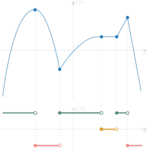
Figure 9.6: An illustration of a function’s right detachment across an interval. The function $f$’s right-detachment is illustrated below the function’s graph.

9.4.3 Mean Value Theorems

In theorem 9.2.2, we formulated an analogue to Fermat’s stationary points theorem. A natural question we may ask is whether other classical results that are applicable to rates calculations, can be reformulated based on trends, with a similar trade off between the information level provided by the theorem and the (broader) set of functions to which it is applicable. Let us first recall the formulation of the following classical results:

Theorem 9.4.3 — Rolle’s theorem. 

Let $f:\left[a,b\right]\rightarrow\mathbb{R}$ be continuous in $\left[a,b\right]$ and differentiable in $\left(a,b\right)$, such that $f\left(a\right)=f\left(b\right).$ Then, there is a point $c\in\left(a,b\right)$ where:

$$\exists\underset{h\rightarrow 0}{\lim}{{f\left(c+h\right)-f\left(c\right)}\over{h}}=0.$$

Theorem 9.4.4 — Lagrange’s mean value theorem. 

Let $f$ be continuous in $\left[a,b\right]$ and differentiable in $\left(a,b\right)$. Then there is $c\in\left(a,b\right)$ with:

$$f^{\prime}\left(c_{v}\right)=\frac{f\left(b\right)-f\left(a\right)}{b-a}.$$

A similar version also exists for integrals:

Theorem 9.4.5 — Mean value theorem for definite integrals. 

Let $f:\left[a,b\right]\rightarrow\mathbb{R}$ be a continuous function. Then there is $c\in\left(a,b\right)$ such that:

$$\int_{a}^{b}f\left(x\right)dx=f\left(c\right)\left(b-a\right).$$

Since the mean value of $f$ on $\left[a,b\right]$ is defined as

$$\frac{1}{b-a}\int_{a}^{b}f\left(x\right)dx,$$

we can interpret the conclusion as $f$ achieves its mean value at some $c\in\left(a,b\right)$.

Inspired by these classical results, let us attempt to suggest their semi-discrete versions.

Theorem 9.4.6 — A semi-discrete Rolle’s theorem. 

Let $f:\left[a,b\right]\rightarrow\mathbb{R}$ be continuous in $\left[a,b\right]$ and detachable in $\left(a,b\right)$ such that $f\left(a\right)=f\left(b\right).$ Then, there is a point $c\in\left(a,b\right)$ where:

$$f_{+}^{;}\left(c\right)+f_{-}^{;}\left(c\right)=0$$

Proof.

$f$ is continuous in a closed interval, hence according to Weierstrass’s theorem, it receives a maximum $M$ and a minimum $m$. In case $m<M$, then, since it is given that $f\left(a\right)=f\left(b\right)$, one of the values $m$ or $M$ must be an image of one of the points in the open interval $\left(a,b\right)$. Let $c\in f^{-1}\left(\left\{M,m\right\}\right)\backslash\left\{a,b\right\}$. $f$ receives a local extremum at $c$. If it is strict, then according to theorem 1, $\exists\underset{h\rightarrow 0}{\lim}\text{sgn}\left[f\left(c+h\right)-f\left(c\right)\right]\neq 0$, hence:

$$f_{+}^{;}\left(c\right)+f_{-}^{;}\left(c\right)=\underset{{\scriptscriptstyle h\rightarrow 0^{+}}}{\lim}\text{sgn}\left[f\left(c+h\right)-f\left(c\right)\right]-\underset{{\scriptscriptstyle h\rightarrow 0^{-}}}{\lim}\text{sgn}\left[f\left(c+h\right)-f\left(c\right)\right]=0,$$

and the claim holds. If the extremum is not strict, then from detachability $f_{+}^{;}\left(c\right)=0$ or $f_{-}^{;}\left(c\right)=0$. If both the one-sided detachments are zeroed then we are done. Otherwise, we assume without loss of generality that $f_{+}^{;}\left(c\right)=0$. Then, $f$ is constant in a right-neighborhood of $c$; hence, $\bar{c}$ for whom $f_{+}^{;}\left(\bar{c}\right)=f_{-}^{;}\left(\bar{c}\right)=0$, and the sum of the one-sided detachments is zeroed trivially. The latter condition also holds trivially in case $m=M$ (where the function is constant). ∎

Theorem 9.4.7 — A semi-discrete Lagrange’s mean value theorem. 

Let $f$ be continuous in $\left[a,b\right]$ and detachable in $\left(a,b\right)$. Assume $f\left(a\right)\neq f\left(b\right).$ Then for each $v\in\left(f\left(a\right),f\left(b\right)\right)$ there is $c_{v}\in f^{-1}\left(v\right)$ with:

$$f^{;}\left(c_{v}\right)=\text{sgn}\left[f\left(b\right)-f\left(a\right)\right].$$

Proof.

Let $v\in\left(f\left(a\right),f\left(b\right)\right).$ Without loss of generality, let us assume that $f\left(a\right)<f\left(b\right)$ and show that there is a point $c_{v}\in f^{-1}\left(v\right)\bigcap\left(a,b\right)$ with $f^{;}_{+}\left(c_{v}\right)=+1.$ From the continuity of $f$ and according to the intermediate value theorem, $f^{-1}\left(v\right)\bigcap\left(a,b\right)\neq\emptyset.$ Assume, on the contrary, that $f_{+}^{;}\left(x\right)=-1$ for each $x\in f^{-1}\left(v\right)\bigcap\left(a,b\right).$ Let $x_{\sup}=\sup\left[f^{-1}\left(v\right)\bigcap\left(a,b\right)\right].$ The maximum is accepted since $f$ is continuous, thus $f\left(x_{\sup}\right)=v.$ According to our assumption, $f_{+}^{;}\left(x_{\sup}\right)=-1,$; hence there is a point $t_{1}>x_{\sup}$ such that $f\left(t_{1}\right)<f\left(x_{\sup}\right)=v.$ But $f$ is continuous in $\left[t_{1},b\right],$; hence, from the intermediate value theorem there is a point $s\in\left(t_{1},b\right)$ for which $f\left(s\right)=v,$ contradicting the selection of $x_{\sup}.$ Had we alternatively assumed that $f_{+}^{;}\left(x_{\sup}\right)=0,$, then there would be a point $t_{2}>x_{\sup}$ for which $f\left(t_{2}\right)=f\left(x_{\sup}\right)=v,$ which again contradicts the selection of $x_{\sup}.$; therefore, $f_{+}^{;}\left(x_{\sup}\right)=+1.$ The proof regarding one-sided left detachments symmetrically leverages the infimum rather than the supremum. ∎

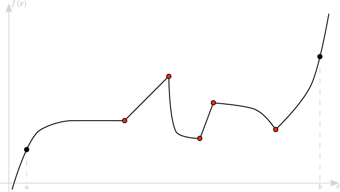
(a) Lagrange’s Mean Value Theorem (theorem 9.4.5) cannot be applied to the illustrated function due to cusp points in its definition domain, where the function is not differentiable.

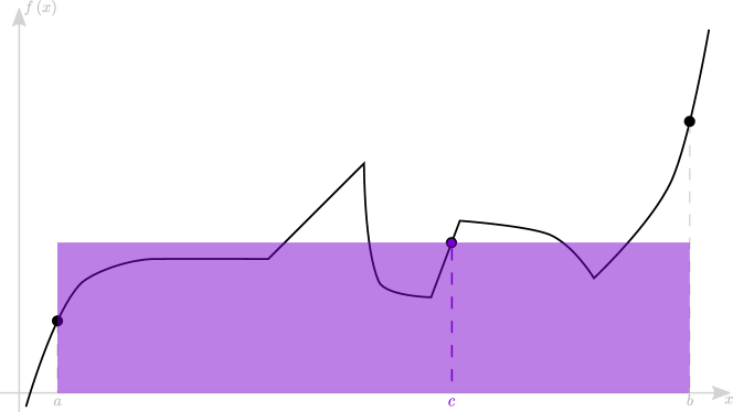
(b) The Mean Value Theorem for Integrals (theorem 9.4.5) can be applied in the domain, and the point $c$ guaranteed by the theorem’s formulation is highlighted.

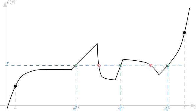
(c) The Mean Value Theorem for Detachments (theorem 9.4.5) can be applied in the domain.

Figure 9.7: Mean Value Theorems for three concepts in Calculus: derivative, integral and detachment.

9.4.4 Detachability and Monotonicity

Detachability is tightly coupled with monotonicity when considered across an interval. The following lemma may be helpful in the below discussion.

Lemma 9.4.4 

A function $f$ is strictly monotonic in an interval if and only if $f$ is continuously detachable and $f^{;}\neq 0$. If the interval is closed with end points $a<b$, then

$$f^{;}=f^{;}_{+}\left(a\right)=f^{;}_{-}\left(b\right).$$

Proof.

First direction. Without loss of generality, assume that $f$ is strictly increasing in the interval. We will show that $f_{-}^{;}=f_{+}^{;}=+1.$ On the contrary, assume without loss of generality that there’s $x$ in the interval for which $f_{+}^{;}\left(x\right)\neq+1.$ According to the definition of the one-sided detachment, it implies that there is a right neighborhood of $x$ such that $f\left(\bar{x}\right)\leq f\left(x\right).$ But $\bar{x}>x,$ contradicting the strict monotonicity.

Second direction. Without loss of generality, let us assume that $f^{;}\equiv+1$ in the interval; then, $f_{+}^{;}=+1$. It must also hold that $f_{-}^{;}=+1$ in the interval, as otherwise, there would exist a point with $f_{-}^{;}=0,$ and $f$ would be constant in the left neighborhood of that point; hence, there would be another point with $f_{+}^{;}=0.$ Let $x_{1},x_{2}\in\left(a,b\right)$ such that $x_{1}<x_{2}.$ We would like to show that $f\left(x_{1}\right)<f\left(x_{2}\right).$ From the definition of the one-sided detachment, there is a left neighborhood of $x_{2}$ such that $f\left(x\right)<f\left(x_{2}\right)$ for each $x$ in that neighborhood. Let $t\neq x_{2}$ be an element of that neighborhood. Let $s=\sup\left\{x|x_{1}\leq x\leq t,f\left(x\right)\geq f\left(x_{2}\right)\right\}.$ On the contrary, let us assume that $f\left(x_{1}\right)\geq f\left(x_{2}\right).$ Then $s\geq x_{1},$ and the supremum exists. If $f\left(s\right)\geq f\left(x_{2}\right)$ (i.e., the supremum is accepted in the defined set), then since for any $x>s$ it holds that $f\left(x\right)<f\left(x_{2}\right)\leq f\left(s\right),$ then $f_{+}^{;}\left(s\right)=-1,$ contradicting $f_{+}^{;}\equiv+1$ in $\left(a,b\right).$ Hence the maximum is not accepted. This implies that $s\neq x_{1}.$ Therefore, according to the definition of the supremum, there is a sequence $x_{n}\rightarrow s$ with $\left\{x_{n}\right\}_{n=1}^{\infty}\subset\left(x_{1},s\right)$ such that: $f\left(x_{n}\right)\geq f\left(x_{2}\right)>f\left(s\right),$ i.e., $f\left(x_{n}\right)>f\left(s\right),$ contradicting our assumption that $f^{;}\left(s\right)=+1$ (which implies that $f_{-}^{;}\left(s\right)\neq-1).$ Hence $f\left(x_{1}\right)<f\left(x_{2}\right).$

If these conditions hold and the interval is closed, then assume without loss of generality that the function strictly increases in the interval. Then, by the definition of the one-sided detachments,

$$f^{;}=f^{;}_{+}\left(a\right)=f^{;}_{-}\left(b\right)=+1.$$

∎

9.4.5 Fundamental Theorem

Let us recall the classic Fundamental Theorem of Calculus.

Theorem 9.4.8 — The fundamental theorem of Calculus. 

The following relations between the fundamental concepts in Calculus hold.

1. Let $f$ be a continuous real-valued function defined on a closed interval $[a,b]$. Let $F$ be the function defined, for all $x\in\left[a,b\right]$ by:

   $${\displaystyle F(x)=\int_{a}^{x}\!f(t)\,dt.}$$

   Then $F$ is uniformly continuous on $[a,b]$ and differentiable on the open interval $(a,b),$ and

   $${\displaystyle F^{\prime}(x)=f(x),\,}\forall\,x\in\left(a,b\right).$$

2. Let $f$ be a real-valued function on a closed interval $\left[a,b\right]$ and $F$ an antiderivative of $f$ in $\left[a,b\right]$: $F^{\prime}(x)=f(x)$. If $f$ is Riemann integrable on $\left[a,b\right]$ then:

   $$\int_{a}^{b}F^{\prime}(x)\,dx=F(b)-F(a).$$

While the detachment is clearly not invertible, it is directly related to the derivative and the integral. The following theorem states these connections and can be thought of as a semi-discrete extension to the fundamental theorem of Calculus.

Theorem 9.4.9 — A semi-discrete extension to the fundamental theorem of Calculus. 

The following relations between the detachment and the fundamental concepts in Calculus hold.

1. Let $f$ be differentiable with a non-vanishing derivative at a point $x$. Then $f$ is detachable and the following holds at $x$:

   $$f^{;}=\text{sgn}\left(f^{\prime}\right).$$

2. Let $f$ be integrable in a closed interval $\left[a,b\right]$. Let $F\left(x\right)\equiv\int_{a}^{x}f\left(t\right)dt$. Let $x\in\left(a,b\right)$. Assume that $f$ is s.c. at $x.$ Then $F$ is detachable and the following holds at $x$:

   $$F^{;}=\text{sgn}\left(f\right).$$

3. Let $f:\mathbb{R}\rightarrow\mathbb{R}$ be continuous in $\left[a,b\right]$ and detachable, then:

   $$\forall v\in\left[f\left(a\right),f\left(b\right)\right]:\,\,\text{sgn}\left[\underset{c_{v}\in f^{-1}\left(v\right)}{\int}f_{\pm}^{;}\left(c_{v}\right)\right]=\text{sgn}\left[f\left(b\right)-f\left(a\right)\right].$$

4. Let $f:\left[a,b\right]\rightarrow\mathbb{R}$ be a continuous function where $f(a)\cdot f(b)\neq 0$. Let $F$ be an antiderivative of $f$ in $\left[a,b\right]$: $F^{\prime}(x)=f(x)$. If $f$ is piecewise monotone on $\left[a,b\right]$, then:

   $$\int_{a}^{b}F^{;}(x)\,dx=b\text{sgn}f\left(b\right)-a\text{sgn}f\left(a\right)-\underset{x_{i}\in f^{-1}\left(0\right)}{\sum}\left[f_{-}^{;}\left(x_{i}\right)+f_{+}^{;}\left(x_{i}\right)\right]x_{i}.$$

Proof.

Let us show each of the statements separately.

1. Let us write the one-sided derivatives’ sign as follows:

   $$\begin{aligned} \text{sgn}\left[f_{\pm}^{\prime}\left(x\right)\right]&=\text{sgn}\left[\underset{h\rightarrow 0^{\pm}}{\lim}\frac{f\left(x+h\right)-f\left(x\right)}{h}\right]=\underset{h\rightarrow 0^{\pm}}{\lim}\text{sgn}\left[\frac{f\left(x+h\right)-f\left(x\right)}{h}\right]\\ &=\pm\underset{h\rightarrow 0^{\pm}}{\lim}\text{sgn}\left[f\left(x+h\right)-f\left(x\right)\right]=f_{\pm}^{;}\left(x\right),\end{aligned}$$ (9.5)

   where the second transition follows from the fact that the derivative is not zeroed, and because the sign function is continuous at $\mathbb{R}\backslash\left\{0\right\}.$

2. Let us apply the following transitions:

   $$\begin{aligned} \text{sgn}\left[f\left(x\right)\right]&=\underset{h\rightarrow 0^{\pm}}{\lim}\text{sgn}\left[f\left(x+h\right)\right]=\pm\underset{h\rightarrow 0^{\pm}}{\lim}\text{sgn}\left[\int_{x}^{x+h}f\left(t\right)dt\right]\\ &=\pm\underset{h\rightarrow 0^{\pm}}{\lim}\text{sgn}\left[F\left(x+h\right)-F\left(x\right)\right]=F_{\pm}^{;}\left(x\right),\end{aligned}$$ (9.6)

   Where the first transition is due to the continuity of $\text{sgn}\left(f\right)$, and the second transition is explained as follows. Assuming $\underset{h\rightarrow 0^{\pm}}{\lim}\text{sgn}\left[f\left(x+h\right)\right]=\Delta_{\pm}$, $f$ maintains the signs $\Delta_{\pm}$ in the one-sided $\delta$-neighborhoods of $x$. Measure theory tells us that the integral $\int_{x}^{x+\delta}f\left(t\right)dt$ also maintains the sign $\Delta_{\pm}$, and

   $$\underset{h\rightarrow 0^{\pm}}{\lim}\text{sgn}\left[\int_{x}^{x+h}f\left(t\right)dt\right]=\pm\Delta_{\pm}.$$

3. If $f\left(a\right)<v<f\left(b\right)$, then consider the function $\widetilde{f}\left(x\right)=\begin{cases}1,&f\left(x\right)>v\\ 0,&f\left(x\right)\leq v\end{cases}$. Sperner’s lemma in one dimension says that if a discrete function takes only the values $0$ and $1$, begins at the value $0$ and ends at the value $1$, then it must switch values an odd number of times. From the continuity of $f$, however, $\widetilde{f}$ switches values in the intersections of $f$ with the line $f=v$. As long as $f\left(x\right)\leq v$, the sum of the one-sided detachments is either $0$ or $+1$. Once $\widetilde{f}$ switches value, the sum of the one-sided detachments is $+2$. Since the switching happens an odd number of times, the final sum is $+2$.

   If $v=f\left(a\right)$ then the above argument yields that the one-sided detachments sum is $+1$.

   If $v=f\left(b\right)$ then define $\utilde{f}\left(x\right)=\begin{cases}1,&f\left(x\right)\geq v\\ 0,&f\left(x\right)<v\end{cases}$ and the above argument applied to $\utilde{f}$ yields that the one-sided detachments sum is $+1$.

4. We first show that given any piecewise continuously detachable function $g:\left[a,b\right]\rightarrow\mathbb{R}$, it holds that:

   $$\int_{a}^{b}g^{;}(x)dx=g_{-}^{;}\left(b\right)b-g_{+}^{;}\left(a\right)a+\underset{1<i<n}{\sum}\left[g_{-}^{;}\left(x_{i}\right)-g_{+}^{;}\left(x_{i}\right)\right]x_{i},$$

   where $\left\{x_{i}\right\}_{i=1}^{n}$ is the set of countable discontinuities of $g^{;}$. $g^{;}$ is integrable as a step function. According to lemma 9.4.4, the detachment is constant in each $\left(x_{i},x_{i+1}\right)$. Thus from known results on integration of step functions in Measure Theory and Calculus:

   $$\int_{a}^{b}g^{;}\left(x\right)dx=\underset{0\leq i\leq n}{\sum}\left(x_{i+1}-x_{i}\right)g_{i}{}^{;},$$

   where $g_{i}{}^{;}$ is the detachment in the (open) $i^{th}$ interval and $x_{0}\equiv a,x_{n+1}\equiv b$. Rearranging the terms and applying the last part of lemma 9.4.4 finalizes the proof. Because $F$ is piecewise monotone, then it is piecewise continuously detachable and we can assign it to $g$ in the later formula. The sign-discontinuities of $f$ are the discontinuities of $F^{;}$. Since $f$ is continuous, then its sign-discontinuities are its zeros. Thus, we also assign in the formula $x_{i}\in f^{-1}\left(0\right)$, the discontinities of $F^{;}$. Hence:

   $$\begin{aligned} &\int_{a}^{b}F^{;}\left(x\right)dx-b\text{sgn}f\left(b\right)+a\text{sgn}f\left(a\right)\\ &=F_{-}^{;}\left(b\right)b-F_{+}^{;}\left(a\right)a+\underset{x_{i}\in f^{-1}\left(0\right)}{\sum}\left[F_{-}^{;}\left(x_{i}\right)-F_{+}^{;}\left(x_{i}\right)\right]x_{i}-b\text{sgn}f\left(b\right)+a\text{sgn}f\left(a\right)\\ &=-\underset{x_{i}\in f^{-1}\left(0\right)}{\sum}\left\{\underset{h\rightarrow 0^{-}}{\lim}\text{sgn}\left[F\left(x_{i}+h\right)-F\left(x_{i}\right)\right]+\underset{h\rightarrow 0^{+}}{\lim}\text{sgn}\left[F\left(x_{i}+h\right)-F\left(x_{i}\right)\right]\right\}x_{i}\\ &=-\underset{x_{i}\in f^{-1}\left(0\right)}{\sum}\left\{\underset{h\rightarrow 0^{-}}{\lim}\text{sgn}\left[\int_{x_{i}}^{x_{i}+h}f\left(t\right)dt\right]+\underset{h\rightarrow 0^{+}}{\lim}\text{sgn}\left[\int_{x_{i}}^{x_{i}+h}f\left(t\right)dt\right]\right\}x_{i}\\ &=-\underset{x_{i}\in f^{-1}\left(0\right)}{\sum}\left\{\underset{t\rightarrow x_{i}^{+}}{\lim}\text{sgn}\left[f\left(t\right)\right]-\underset{t\rightarrow x_{i}^{-}}{\lim}\text{sgn}\left[f\left(t\right)\right]\right\}x_{i}\\ &=-\underset{x_{i}\in f^{-1}\left(0\right)}{\sum}\left\{\underset{t\rightarrow x_{i}^{+}}{\lim}\text{sgn}\left[f\left(t\right)-f\left(x_{i}\right)\right]-\underset{t\rightarrow x_{i}^{-}}{\lim}\text{sgn}\left[f\left(t\right)-f\left(x_{i}\right)\right]\right\}x_{i}\\ &=-\underset{x_{i}\in f^{-1}\left(0\right)}{\sum}\left[f_{+}^{;}\left(x_{i}\right)+f_{-}^{;}\left(x_{i}\right)\right]x_{i},\end{aligned}$$ (9.7)

   where the second transition is due to the definition of the detachment and part 2 of this theorem; the third transition is due to the second part of the Fundamental Theorem of Calculus; the fourth transition is due to considerations similar to these applied in the proof of this theorem’s second part; the fifth transition is due to $f$ being zeroed at the points $x_{i}$; and the sixth transition is due to the definition of the detachment. Note that, for convenience, in the proof above we assumed that the function’s zeros is a countable set. However, the formula clearly holds also for functions with uncountable zeros.

∎

The first part of theorem 9.4.9 shows that the detachment operator coincides with the derivative sign whenever a function has a non-zeroed derivative; hence this operator’s mathematical power lies mostly in the cases where the derivative is zeroed or undefined.

The fourth part of theorem 9.4.9 is the only result in this book that incorporates all these concepts together: differentiability, integrability, sign-continuity, monotonicity, and detachability.

9.4.6 Composite and Inverse Functions Rules

Recall the chain rule in Differential Calculus:

Claim 9.4.5 

Chain rule. If $g$ is a function that is differentiable at a point $c$ (i.e. the derivative $g^{\prime}\left(c\right)$ exists) and $f$ is a function that is differentiable at $g\left(c\right)$, then the composite function $f\circ g$ is differentiable at $c$, and:

$$\left(f\circ g\right)^{\prime}\left(c\right)=f^{\prime}\left(g\left(c\right)\right)\cdot g^{\prime}\left(c\right).$$

Let us formulate its semi-discrete analogue that allows to calculate trends of composite, not necessarily differentiable, functions.

Claim 9.4.6 

A semi-discrete chain rule. If $g$ is continuous and detachable at $x$, and $f$ is detachable at $g\left(x\right)$, then $f\circ g$ is detachable at $x$ and the following holds there:

$$\left(f\circ g\right)^{;}=\left(f^{;}\circ g\right)g^{;}.$$

Proof.

By separating to cases. Without loss of generality, let us limit our discussion to right-detachments, and assume $g_{+}^{;}\left(x\right)=f_{+}^{;}\left(g\left(x\right)\right)=+1.$

According to the definition of the detachment of $f$ at $g\left(x\right)$:

$$\exists\delta_{f}:0<\bar{t}-g\left(x\right)<\delta_{f}\Longrightarrow f\left(g\left(x\right)\right)<f\left(\bar{t}\right).$$

Further, according to the definition of the detachment and the continuity of $g$:

$$\forall\epsilon,\,\exists\delta_{g}:0<\bar{x}-x<\delta_{g}\Longrightarrow 0<g\left(\bar{x}\right)-g\left(x\right)<\epsilon.$$

Therefore, for $\epsilon\equiv\delta_{f}$ it holds that:

$$\exists\delta_{g}:0<\bar{x}-x<\delta_{g}\Longrightarrow 0<g\left(\bar{x}\right)-g\left(x\right)<\delta_{f}\Longrightarrow f\left(g\left(x\right)\right)<f\left(g\left(\bar{x}\right)\right),$$

hence $\left(f\left(g\left(x\right)\right)\right)^{;}=+1.$ The rest of the cases are handled similarly. ∎

Recall the inverse function rule for derivatives:

Claim 9.4.7 

Inverse function rule. If $g$ is a function that is differentiable at a point $c$ (i.e. the derivative $g^{\prime}\left(c\right)$ exists) and $f$ is a function that is differentiable at $g\left(c\right)$, then the composite function $f\circ g$ is differentiable at $c$, and:

$$\left(f\circ g\right)^{\prime}\left(c\right)=f^{\prime}\left(g\left(c\right)\right)\cdot g^{\prime}\left(c\right).$$

Let us suggest a semi-discrete analogue for the detachment operator:

Claim 9.4.8 

A semi-discrete inverse function rule. A function $f:A\rightarrow\mathbb{R}$ is continuously detachable at $a\in A$ and $f^{;}\left(a\right)\neq 0$, if and only if $f$ is invertible in a neighborhood of $a$. It then holds that $f^{-1}$ is continuously detachable at a neighborhood of $f\left(a\right)$ and:

$$\left(f^{-1}\right)^{;}\left(f\left(a\right)\right)=f^{;}\left(a\right)$$

Proof.

First direction. Since $f^{;}\neq 0$ is continuous then either $f^{;}\equiv+1$ or $f^{;}\equiv-1$ in a neighborhood of $a.$ According to lemma 9.4.4, $f$ is thus strictly monotonic in that neighborhood. Without loss of generality assume that $f$ is strictly increasing. Then $x<y\Longleftrightarrow f\left(x\right)<f\left(y\right).$ Thus $f^{-1}\left(x\right)<f^{-1}\left(y\right)\Longleftrightarrow x<y.$ According to the second direction of lemma 9.4.4, $\left(f^{-1}\right)^{;}\equiv+1.$

Second direction. $f$ is invertible, hence strictly monotonic. According to lemma 9.4.4, $f^{;}\neq 0$ is continuous.

Under those conditions, both $f$ and $f^{\left(-1\right)}$ are monotonic in the neighborhood of the points at stake, and, according to lemma 9.4.4, they are continuously detachable. ∎

Another useful result is the following functional power rule in Differential Calculus:

Claim 9.4.9 

Functional Power Rule. Given a base function $f$ and an exponent function $g$, if:

1. The power function $f^{g}$ is well-defined at a point $x$ (particularly $f\left(x\right)>0$)

2. $f$ and $g$ are both differentiable

Then the function $f^{g}$ is differentiable and:

$$\left(f^{g}\right)^{\prime}=f^{g}\left(g^{\prime}\ln f+f^{\prime}\frac{g}{f}\right).$$

Let us suggest its semi-discrete analogue as follows:

Claim 9.4.10 

A semi-discrete functional power rule. Given a base function $f$, an exponent function $g$, and a point $x$ in their definition domain, if the following conditions hold:

1. The power function $f^{g}$ is well-defined (particularly $f\left(x\right)>0$)

2. $f$ and $g$ are both detachable and sign-consistent

3. Either:

   • $f^{;}g^{;}\left(f-1\right)g\geq 0$, where $f$ or $g$ is s.c., or $f=1$ and $g=0$, or:

   • $f^{;}g^{;}\left(f-1\right)g<0$, where $f$ or $g$ is s.d.

Then the function $f^{g}$ is detachable and:

$$\left(f^{g}\right)^{;}=\begin{cases}\left[\left(f-1\right)g\right]^{;},&gg^{;}\left(f-1\right)f^{;}\geq 0,\text{ and }f-1\text{ or }g\text{ is s.c.}\\ f^{;}g^{;},&\text{else.}\end{cases}$$

Proof.

The claim follows from the following transitions:

$$\begin{aligned} \left(f^{g}\right)^{;}&=\left(e^{g\ln f}\right)^{;}=\left(g\ln f\right)^{;}\\ &=\begin{cases}\text{sgn}\left[g^{;}\text{sgn}\left(\ln f\right)+\left(\ln f\right)^{;}\text{sgn}\left(g\right)\right],&gg^{;}\ln f\left(\ln f\right)^{;}\geq 0\text{, and }g\text{ or }\ln f\text{ is s.c.}\\ f^{;}g^{;},&\text{else}\end{cases}\\ &=\begin{cases}\text{sgn}\left[g^{;}\text{sgn}\left(f-1\right)+f^{;}\text{sgn}\left(g\right)\right],&gg^{;}\left(f-1\right)f^{;}\geq 0\text{, and }g\text{ or }f-1\text{ is s.c.}\\ f^{;}g^{;},&\text{else}\end{cases}\\ &=\begin{cases}\text{sgn}\left[g^{;}\text{sgn}\left(f-1\right)+\left(f-1\right)^{;}\text{sgn}\left(g\right)\right],&gg^{;}\left(f-1\right)f^{;}\geq 0\text{, and }g\text{ or }f-1\text{ is s.c.}\\ f^{;}g^{;},&\text{else}\end{cases}\\ &=\begin{cases}\left[\left(f-1\right)g\right]^{;},&gg^{;}\left(f-1\right)f^{;}\geq 0,\text{ and }f-1\text{ or }g\text{ is s.c.}\\ f^{;}g^{;},&\text{else.}\end{cases}\end{aligned}$$ (9.8)

where the second transition is due to the strict monotonicity of the exponent function, the third transition is due to the product rule (claim 2), the fourth is since $\text{sgn}\left[\ln\left(f\right)\right]=\text{sgn}\left(f-1\right)$, and due to the strict monotonicity of the natural logarithm function, the fifth is due to claim 9.4.1, and the sixth is due to claim 2 again. ∎

A simulation of the functional power rule is available. Note that this rule forms another example of the detachment’s numerical efficiency with respect to that of the derivative sign. The functional power rule for derivatives yields a formula that involves logarithms and division. Instead, the rule above, while appears to be more involved on the paper because of the conditions, may be more efficient computationally-wise, depending on the setting.

9.5 Theoretical Applications

9.5.1 Limits and Trends Evaluation Tools

Let us recall the Taylor series formulation.

Theorem 9.5.1 — Taylor series. 

The Taylor series of a real or complex-valued function $f$ that is infinitely differentiable at a real or complex number $a$ is the power series

$$f\left(x\right)=f\left(a\right)+\frac{f^{\prime}\left(a\right)}{1!}\left(x-a\right)+\frac{f^{\prime\prime}\left(a\right)}{2!}\left(x-a\right)^{2}+\frac{f^{\prime\prime\prime}\left(a\right)}{3!}\left(x-a\right)^{3}+\ldots=\underset{n}{\sum}\frac{f^{\left(n\right)}\left(a\right)}{n!}\left(x-a\right)^{n},$$

where $f^{\left(n\right)}\left(a\right)$ denotes the $n^{th}$ derivative of $f$ evaluated at the point $a$.

The following semi-discrete reformulation of Taylor’s theorem expresses the trend given rates concisely. It may also be thought of as an interim step towards proving known Calculus claims about stationary points classification.

Corollary 9.5.1 

A semi-discrete rearrangement of Taylor series. If $f\not\equiv 0$ is differentiable infinitely many times at $x$, and detachable, then the detachment of $f$ is calculated as follows:

$$f_{\pm}^{;}\left(x\right)=\left(\pm 1\right)^{k+1}\text{sgn}\left[f^{\left(k\right)}\left(x\right)\right],$$

where $f^{\left(i\right)}$ represents the $i^{th}$ derivative, and $k=\min\left\{i\in\mathbb{N}|f^{\left(i\right)}\left(x\right)\neq 0\right\}$, if there exists such $k$.

Proof.

The first equality is obtained from the Taylor series:

$$f(x+h)=f(x)+hf^{\prime}(x)+\frac{h^{2}}{2}f^{\prime\prime}(x)+\frac{h^{3}}{6}f^{(3)}(x)+\ldots$$

by simple algebraic manipulations followed by applying the limit process.

The second equality holds due to the following analysis:

$$\begin{aligned} \underset{{\scriptscriptstyle h\rightarrow 0^{\pm}}}{\lim}\text{sgn}\left[\underset{{\scriptscriptstyle i\in\mathbb{N}}}{\overset{}{\sum}}\frac{h^{i-1}}{i!}f_{\pm}^{\left(i\right)}\left(x\right)\right]&=\underset{{\scriptscriptstyle h\rightarrow 0^{\pm}}}{\lim}\text{sgn}\left[\frac{h^{k-1}}{k!}f^{\left(k\right)}\left(x\right)+\mathcal{O}\left(h^{k}\right)\right]\\ &=\underset{{\scriptscriptstyle h\rightarrow 0^{\pm}}}{\lim}\text{sgn}\left[\frac{h^{k-1}}{k!}f^{\left(k\right)}\left(x\right)\right]=\left(\pm 1\right)^{k+1}\text{sgn}\left[f^{\left(k\right)}\left(x\right)\right],\end{aligned}$$ (9.9)

where the second equality holds because for a sufficiently small $h$, we have that

$$\text{sgn}\left[\frac{h^{k-1}}{k!}f^{\left(k\right)}\left(x\right)+\mathcal{O}\left(h^{k}\right)\right]=\text{sgn}\left[\frac{h^{k-1}}{k!}f^{\left(k\right)}\left(x\right)\right].$$

The final step is obtained by keeping in mind the limit’s side and the parity of $k$. ∎

Note that claim 9.4.2 and theorems 2 and 9.4.2 (the sum and difference, product and quotient rules, respectively) impose varied conditions. However, in the special case that the functions $f,g$ are both detachable and differentiable infinitely many times, the following corollaries from claim 9.5.1 hold independently of these conditions:

1. If $f+g$ is detachable, then

   $$\left(f+g\right)_{\pm}^{;}=\left(\pm 1\right)^{k+1}\text{sgn}\left[f^{\left(k\right)}+g^{\left(k\right)}\right],$$

   where $k\equiv\min\left\{i\in\mathbb{N}|f^{\left(i\right)}\neq-g^{\left(i\right)}\right\}$ . An analogous statement holds for the difference $f-g$.

2. If $fg$ is detachable, then

   $$\left(fg\right)_{\pm}^{;}=\left(\pm 1\right)^{k+1}\text{sgn}\left[f^{\left(k\right)}g+fg^{\left(k\right)}\right],$$

   where $k\equiv\min\left\{i\in\mathbb{N}|f^{\left(i\right)}g\neq-fg^{\left(i\right)}\right\}.$ An analogous statement holds for the difference $\frac{f}{g}$.

For example, consider the functions $f\left(x\right)=x^{2},g\left(x\right)=-x^{4}$ at $x=0$. Rule 3 does not yield an indication regarding $\left(f+g\right)^{;}$ since $f^{;}g^{;}=-1\notin\left\{0,1\right\}$. However, the aforementioned statement lets us know that $\left(f+g\right)_{\pm}^{;}\left(x\right)=\left(\pm 1\right)^{2+1}\text{sgn}\left[2+0\right]=\pm 1$.

Recall L’Hôpital Rule that serves as a convenient limit evaluations tool.

Theorem 9.5.2 — L’Hôpital rule. 

Given functions $f$ and $g$ which are differentiable on an open interval $I$ except possibly at a point $c$ contained in $I$, if for all $x$ in $I$ with $x\neq c$:

1. $\lim_{x\to c}f(x)=\lim_{x\to c}g(x)=0{\text{ or }}\pm\infty$

2. $g^{\prime}(x)\neq 0$

3. $\exists\lim_{x\to c}{\frac{f^{\prime}(x)}{g^{\prime}(x)}}$

Then:

$$\lim_{x\to c}{\frac{f(x)}{g(x)}}=\lim_{x\to c}{\frac{f^{\prime}(x)}{g^{\prime}(x)}}.$$

Let us suggest its semi-discrete analogue as follows.

Theorem 9.5.3 — A semi-discrete L’Hôpital rule. 

Let $f,g:\mathbb{R}\rightarrow\mathbb{R}$ be a pair of functions and a point $x$ in their definition domain. Assume that $\underset{t\rightarrow x^{\pm}}{\lim}f^{;}\left(t\right)$ and $\underset{t\rightarrow x^{\pm}}{\lim}g^{;}\left(t\right)$ exist. If $\underset{t\rightarrow x^{\pm}}{\lim}\left|f\left(t\right)\right|=\underset{t\rightarrow x^{\pm}}{\lim}\left|g\left(t\right)\right|\in\left\{0,\infty\right\},$ then:

$$\underset{t\rightarrow x^{\pm}}{\lim}\text{sgn}\left[f\left(t\right)g\left(t\right)\right]=\underset{t\rightarrow x^{\pm}}{\lim}f^{;}\left(t\right)g^{;}\left(t\right).$$

Proof.

We prove a slightly more generic claim: Let $\left\{f_{i}:\mathbb{R}\rightarrow\mathbb{R}\right\}_{1\leq i\leq n}$ be a set of functions and a point $x$ in their definition domain. Assume that $\underset{t\rightarrow x^{\pm}}{\lim}f_{i}^{;}\left(t\right)$ exist for each $i.$ If $\underset{t\rightarrow x^{\pm}}{\lim}\left|f_{i}\left(t\right)\right|=L\in\left\{0,\infty\right\},$ then we will show that:

$$\underset{t\rightarrow x^{\pm}}{\lim}\text{sgn}\underset{i}{\prod}f\left(t\right)=\left(\pm C\right)^{n}\underset{t\rightarrow x^{\pm}}{\lim}\underset{i}{\prod}f^{;}\left(t\right),$$

where $C$ equals $+1$ or $-1$ if $\underset{t\rightarrow x^{\pm}}{\lim}\left|f_{i}\left(t\right)\right|$ is $0$ or $\infty,$ to which we refer below as part 1 and 2, respectively.

We apply induction on $n.$ Let $n=1,$ and for simplicity denote $f=f_{1}.$ Without loss of generality we focus on right limits and assume that $\underset{t\rightarrow 0^{+}}{\lim}f^{;}\left(t\right)=+1.$ Then $f^{;}=+1$ for each point in a right $\delta$-neighborhood of $x.$ According to lemma 9.4.4, $f$ is strictly increasing in $\left(x,x+\delta\right).$ Therefore:

$$\inf\left\{f\left(t\right)|t\in\left(x,x+\delta\right)\right\}=\underset{t\rightarrow x^{+}}{\lim}f\left(t\right).$$

Proof of Part 1. According to our assumption, $\inf\left\{f\left(t\right)|t\in\left(x,x+\delta\right)\right\}=0.$ Thus $f\left(t\right)\geq 0$ for $t\in\left(x,x+\delta\right).$ Clearly, $f$ cannot be zeroed in $\left(x,x+\delta\right)$ because that would contradict the strict monotony. Thus $f>0$ there, and $\underset{t\rightarrow x^{+}}{\lim}\text{sgn}f\left(t\right)=\underset{t\rightarrow x^{+}}{\lim}f^{;}\left(t\right)=+1.$ If $\underset{t\rightarrow x^{+}}{\lim}f^{;}\left(t\right)=0,$ then $f$ is constant in a right-neighborhood of $x,$ and from the continuity $f\equiv 0$. Thus $\underset{t\rightarrow x^{+}}{\lim}\text{sgn}f\left(t\right)=\underset{t\rightarrow x^{+}}{\lim}f_{+}^{;}\left(t\right)=0.$ The signs switch for left-limits, hence the $\pm$ coefficient in the right handside.

Proof of Part 2. Since $f$ is strictly increasing in a right-neighborhood of $x,$, then $\underset{t\rightarrow x^{+}}{\lim}f\left(t\right)=-\infty,$ and $\underset{t\rightarrow x^{+}}{\lim}\text{sgn}f\left(t\right)=-\underset{t\rightarrow x^{+}}{\lim}f^{;}\left(t\right)=-1.$ The signs switch for left-limits, hence the $\mp$ coefficient in the right handside.

Assume that the theorem holds for $n,$ and we show its correctness for $n+1$:

$$\begin{aligned} \underset{t\rightarrow x^{\pm}}{\lim}\text{sgn}\underset{i}{\prod}f_{i}\left(t\right)&=\underset{t\rightarrow x^{\pm}}{\lim}\text{sgn}\underset{i}{\prod}f_{i}\left(t\right)\cdot\underset{t\rightarrow x^{\pm}}{\lim}\text{sgn}f_{n+1}\left(t\right)\\ &=\left(\pm C\right)^{n}\underset{t\rightarrow x^{\pm}}{\lim}\underset{i}{\prod}f_{i}^{;}\left(t\right)\cdot\underset{t\rightarrow x^{\pm}}{\lim}\text{sgn}f_{n+1}\left(t\right)\\ &=\left(\pm C\right)^{n+1}\underset{t\rightarrow x^{\pm}}{\lim}\underset{i}{\prod}f_{i}^{;}\left(t\right),\end{aligned}$$ (9.10)

where the second transition follows from the induction hypothesis, and the third follows from the induction base. ∎

Without assuming that the conditions stated in claim 9.4.2 and 2, detachable functions’ sum and product are not even guaranteed to be detachable. For example, consider the right-detachable pair of functions at $x=0$:

$$g_{1}\left(x\right)=\begin{cases}1,&x>0\\ 0,&x=0\end{cases},\qquad,g_{2}\left(x\right)=\begin{cases}1,&x\in\mathbb{Q^{+}}\\ -1,&x\in\mathbb{R^{+}\backslash\mathbb{Q}}\\ 2,&x=0,\end{cases}$$

whose sum and product are not detachable at zero. Counterexamples exist even if we assume differentiability on top of detachability. Discarding the continuity assumption on $g$ in claim 9.4.6 may result in a non-detachable $f\circ g$, for example at $x=0$ for the pair of functions $f\left(x\right)=x^{2}$ and:

$$g\left(x\right)=\begin{cases}\left|\sin\left(\frac{1}{x}\right)\right|,&x\neq 0,\\ -\frac{1}{2},&x=0.\end{cases}$$

We finalize this subsection with a simple criterion for constancy in an interval containing a point.

Claim 9.5.2 

$f:\mathbb{R}\rightarrow\mathbb{R}$ is constant in the neighborhood of $x_{0}$ if and only if $f_{\pm}^{;}\left(x_{0}\right)=0$.

Proof.

First direction. Assume that $f_{\pm}^{;}=0$. Then:

$$\forall\epsilon>0,\exists\delta>0:\quad\left|x-x_{0}\right|<\delta\quad\Longrightarrow\quad\left|\text{sgn}\left[f\left(x\right)-f\left(x_{0}\right)\right]-0\right|<\epsilon,$$

hence

$$\left|\text{sgn}\left[f\left(x\right)-f\left(x_{0}\right)\right]\right|<\epsilon,$$

which particularly holds for $\epsilon=\frac{1}{2}$. The only option is $\text{sgn}\left[f\left(x\right)-f\left(x_{0}\right)\right]=0$, which implies $f\left(x\right)=f\left(x_{0}\right)$ for the $\delta$-neighborhood of $x_{0}$, resulting with $f$ constant.

Second direction. Let $\delta$ be small enough such that $f$ is constant in $B_{\delta}\left(x_{0}\right)=\left(x_{0}-\delta,x_{0}+\delta\right)$, and let $\epsilon>0$. Let $x\in B_{\delta}\left(x_{0}\right)$. Then:

$$\left|\text{sgn}\left[f\left(x\right)-f\left(x_{0}\right)\right]-0\right|=0<\epsilon.$$

∎

9.5.2 Detachment Test

In this subsection we mirror several derivative tests in terms of the detachment and suggest that the detachment version may be occasionally beneficial, for example, in case a given function is detachable but not differentiable.

Recall the first derivative test:

Claim 9.5.3 

First derivative test. Suppose $f$ is a real-valued function of a real variable defined on some interval containing the critical point $a$. Furthermore, suppose that $f$ is continuous at $a$ and differentiable on some open interval containing $a$, except, perhaps, at $a$ itself.

• If there is a positive number $r>0$ such that for every $x\in\left(a-r,a\right)$ we have $f^{\prime}\left(x\right)\geq 0$ ($f^{\prime}\left(x\right)\geq 0$), and for every $x\in\left(a,a+r\right)$ we have $f^{\prime}\left(x\right)\leq 0$ ($f^{\prime}\left(x\right)\leq 0$), then $f$ has a local maximum (minimum) at $a$.

• If there is a positive number $r>0$ such that for every x in $\left(a-r,a\right)\bigcup\left(a,a+r\right)$ we have $f^{\prime}\left(x\right)>0$ ($f^{\prime}\left(x\right)<0$), then $f$ is strictly increasing (decreasing) at $a$ and has neither a local maximum nor a local minimum.

• If none of the above conditions hold, then the test fails.

A detachment-based version of the first derivative test does not require continuity and provides both sufficient and necessary conditions.

Claim 9.5.4 

First detachment test. Suppose $f$ is a real-valued function of a real variable defined on some interval containing the point $a$. Furthermore, suppose that $f$ is detachable at $a$. Then:

• $f_{\pm}^{;}\left(x\right)\in\left\{0,\mp 1\right\}$ ($f_{\pm}^{;}\left(x\right)\in\left\{0,\pm 1\right\}$) respectively, if and only if $f$ has a local maximum (minimum) at $a$.

• $f^{;}\left(x\right)\equiv+1$ ($f^{;}\left(x\right)=-1$) respectively in a neighborhood of $a$, if and only if $f$ is strictly increasing (decreasing) at $a$ and has neither a local maximum nor a local minimum.

Proof.

Without loss of generality, we prove the claim for maxima and strict increasing points.

• The condition $f_{\pm}^{;}\left(a\right)\in\left\{0,\mp 1\right\}$, is equivalent, by the definition on the one-sided detachment, to the existence of left and right neighborhoods of $a$, $B_{r^{-}}\left(a\right)$ and $B_{r^{+}}\left(a\right)$ respectively, such that:

  $$\forall x_{-}\in B_{r^{-}}\left(a\right):\quad -sgn\left[f\left(x_{-}\right)-f\left(a\right)\right]\in\left\{0,+1\right\}$$

  $$\forall x_{+}\in B_{r^{+}}\left(a\right):\quad sgn\left[f\left(x_{+}\right)-f\left(a\right)\right]\in\left\{0,-1\right\},$$

  which is equivalent to the following condition:

  $$\forall x\in B_{r^{\pm}}\left(a\right):\quad f\left(x\right)\leq f\left(a\right),$$

  that coincides with the definition of a local maximum.

• By the lemma 9.4.4, $f^{;}\left(x\right)\equiv+1$ in an interval if and only if $f$ is strictly increasing. Therefore, this property in an open neighborhood of $a$ is a sufficient and necessary condition for $f$ to strictly increase at $a$.

∎

Similarly, we may mirror the second derivative test.

Claim 9.5.5 

Second-derivative test. If the function $f$ is twice-differentiable at a critical point $x$ (i.e. a point where $f^{\prime}\left(x\right)=0$), then:

• If $f^{\prime\prime}\left(x\right)<0$, then $f$ has a local maximum at $x$.

• If $f^{\prime\prime}\left(x\right)>0$, then $f$ has a local minimum at $x$.

• If $f^{\prime\prime}\left(x\right)=0$, the test is inconclusive.

Claim 9.5.6 

Second-detachment test. If the derivative of the function $f$ is detachable at a critical point $x$, then:

• If $f^{\prime;}\left(x\right)=-1$, then $f$ has a local maximum at $x$.

• If $f^{\prime;}\left(x\right)=+1$, then $f$ has a local minimum at $x$.

• If $f^{\prime;}\left(x\right)=0$, then $f$ has both a local minimum and maximum at $x$ (it is constant in its neighborhood).

Proof.

Let us prove the first and third statements:

• $f^{\prime;}\left(x\right)=-1$ implies that $\pm\underset{x\to x_{0}^{\pm}}{\lim}\text{sgn}\left[f^{\prime}\left(x\right)-f^{\prime}\left(x_{0}\right)\right]=-1$. Since $x_{0}$ is a critical point, $f^{\prime}\left(x_{0}\right)=0$ (by definition). Therefore according to the limit definition, for all $x_{-}$ in some left-neighborhood of $x_{0}$, it holds that $\text{sgn}\left[f^{\prime}\left(x_{-}\right)\right]=+1$, or $f^{\prime}\left(x_{-}\right)>0$; and for all $x_{+}$ in some right-neighborhood of $x_{0}$, it holds that $\text{sgn}\left[f^{\prime}\left(x_{+}\right)\right]=-1$, or $f^{\prime}\left(x_{+}\right)<0$. Hence, according to the first derivative test, $f$ has a local maximum at $x$.

• $f^{\prime;}\left(x\right)=0$ implies that $\underset{x\to x_{0}^{\pm}}{\lim}\text{sgn}\left[f^{\prime}\left(x\right)\right]=0$, hence $f^{\prime}$ is zeroed in a neighborhood of $x$, and $f$ is thus constant.

∎

Similarly, one may apply the one-sided detachments as a concise sufficient condition upon analyzing inflection points. As stated in [144], the existence of an inflection point $x_{0}$ is guaranteed if the sign of the second derivative changes while traversing from the left neighborhood of $x_{0}$ to the right, if there is also a tangent at the point. As such, the question of whether the curve has an inflection point can be answered by checking the sign of the second derivative traversing the considered point. This condition may be further alleviated: we do not require that the function is differentiable twice, but solely that its derivative is detachable. We add to that the following condition:

$$\begin{cases}\left(\frac{df}{dx}\right)_{+}^{;}\left(x_{0}\right)+\left(\frac{df}{dx}\right){}_{-}^{;}\left(x_{0}\right)=0\\ \left(\frac{df}{dx}\right)_{+}^{;}\left(x_{0}\right)\cdot\left(\frac{df}{dx}\right)_{-}^{;}\left(x_{0}\right)\neq 0.\end{cases}$$

9.5.3 Calculating Instantaneous Trends in Practice

Let us calculate the detachments directly according to the detachment definition, or according to corollary 9.5.1. In the following examples, we scrutinize cases where the detachable functions are either continuous but not differentiable, discontinuous, or differentiable. As a side note, we also examine a case where the trend does not exist.

Let $g\left(x\right)=\sqrt{\left|x\right|}$ which is not differentiable at zero. Then we can calculate the trend directly from the detachment definition:

$$\begin{aligned} g_{\pm}^{;}\left(x\right)&=\pm\underset{h\rightarrow 0^{\pm}}{\lim}\text{sgn}\left(\sqrt{\left|x+h\right|}-\sqrt{\left|x\right|}\right)=\pm\underset{h\rightarrow 0^{\pm}}{\lim}\text{sgn}\left[\left(x+h\right)^{2}-x^{2}\right]\\ &=\pm\underset{h\rightarrow 0^{\pm}}{\lim}\text{sgn}\left[h\left(2x+h\right)\right]=\begin{cases}\text{sgn}\left(x\right),&x\neq 0\\ \pm 1,&x=0\end{cases}\end{aligned}$$ (9.11)

That is, the one-sided detachments are positive at zero, indicating a minimum. At points other than zero, we see that the detachment’s values agree with the derivative’s sign, as expected from part 1 of theorem claim 9.4.9. Weirstrass function, which is nowhere differentiable, can be shown to be detachable at infinitely many points with similar means.

Next, let the sign function $\ell\left(x\right)=\text{sgn}\left(x\right)$ (not to be confused with the definition of the detachment), which is discontinuous at $x=0$. Then, its trends can be concisely evaluated by the definition:

$$\ell_{\pm}^{;}\left(x\right)=\pm\underset{{\scriptscriptstyle h\rightarrow 0^{\pm}}}{\lim}\text{sgn}\left[\text{sgn}\left(x+h\right)-\text{sgn}\left(x\right)\right]=\begin{cases}0,&x\neq 0\\ \pm\underset{{\scriptscriptstyle h\rightarrow 0^{\pm}}}{\lim}\text{sgn}\left(h\right)=+1,&x=0\end{cases}$$

Finally, let us calculate trends based on claim 9.5.1 (in case the function is differentiable infinitely many times). Those are the explicit calculations that are otherwise obfuscated by Taylor series based theorems on critical points classification. For instance, consider the function $f\left(x\right)=-3x^{5}+5x^{3},$ whose critical points are at $0,\pm 1$:

$$\begin{aligned} f_{\pm}^{;}\left(x\right)&=\left(\pm 1\right)^{k+1}\text{sgn}\left[f^{\left(k\right)}\left(x\right)\right]\\ f_{\pm}^{;}\left(0\right)&=\left(\pm 1\right)^{3+1}\text{sgn}\left(5\right)=+1\\ f_{\pm}^{;}\left(-1\right)&=\left(\pm 1\right)^{2+1}\text{sgn}\left(15\right)=\pm 1\\ f_{\pm}^{;}\left(1\right)&=\left(\pm 1\right)^{2+1}\text{sgn}\left(-15\right)=\mp 1,\end{aligned}$$ (9.12)

where the transition on the first raw is due to claim 9.5.1. We know that $0,+1$ and $-1$ are inflection, maximum and minimum points, respectively.

For completeness, let us show that the trend does not exist for the function

$$s\left(x\right)=\begin{cases}\sin\left(\frac{1}{x}\right),&x\neq 0\\ 0,&x=0,\end{cases}$$

at $x=0$. We present two different sequences whose limit is zero:

$$a_{n}=\left\{\frac{2}{\pi\left(1+4n\right)}\right\},b_{n}=\left\{\frac{1}{\pi\left(1+2n\right)}\right\}.$$

As the sine function is constant for both sequences ($1$ and $0$ respectively), then so is the limit of the change’s sign, which equals $+1$ and $0$ for $a_{n}$ and $b_{n}$, respectively. Heine’s limit definition doesn’t hold, so $s$ isn’t detachable. Indeed, this function’s instantaneous trend is non existent at $x=0$.

9.6 Exercises

Prove or refute the following claims, that are based on the counter examples illustrated in [533]. Let us assume in all the below examples that $f,g$ are functions whose domains and images are $\mathbb{R}$ unless specified otherwise. The solutions are listed in the following subsection.

Exercise 9.1 

If $\left|f\right|$ is detachable at $x$ then so is $f$. $\blacksquare$

Counter example: $f\left(x\right)=\left(-1\right)^{\boldsymbol{1}_{\mathbb{Q}}}$. $\left|f\right|\equiv+1$ is detachable, but $f$ oscillates indefinitely between $-1$ and $+1$ and is, therefore, particularly nowhere detachable.

Figure 9.8: An illustration of a function refuting the claim in exercise 9.1

Exercise 9.2 

If $f,g$ are not detachable at $x$ then so is $f+g$. $\blacksquare$

Counter example: Any non-detachable function $f$ and its additive inverse $-f$ refute the claim.

Exercise 9.3 

If $f,g$ are not detachable at $x$ so is $f\cdot g$. $\blacksquare$

Counter example: $f\left(x\right)=\left(-1\right)^{\boldsymbol{1}_{\mathbb{Q}}}$ and $g\left(x\right)=\left(-1\right)^{1+\boldsymbol{1}_{\mathbb{Q}}}$ are not detachable, however $\left(f\cdot g\right)\left(x\right)\equiv-1$ is detachable.

Exercise 9.4 

If $f$ is detachable in the neighborhood of $a\in\mathbb{R}$, including at $a$, and:

$$f^{;}\left(x\right)=\begin{cases}+1,&x<a\\ -1,&x>a,\end{cases}$$

then $f$ incurs a local maximum at $x=a$. $\blacksquare$

Counter example: $a=0$ with the following function:

$$f\left(x\right)=\begin{cases}\frac{1}{x^{2}},&x\neq 0\\ 0,&x=0.\end{cases}$$

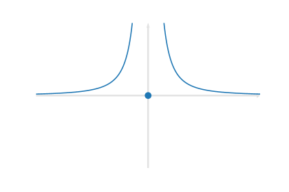
Figure 9.9: An illustration of a function refuting the claim in exercise 9.4

Exercise 9.5 

$f$ cannot be detachable only at a single point $a$. $\blacksquare$

Counter example: The following function is detachable only at $a=0$:

$$f\left(x\right)=\begin{cases}\left(-1\right)^{\boldsymbol{1}_{\mathbb{Q}}},&x\neq 0\\ 2,&x=0.\end{cases}$$

Exercise 9.6 

If $f,g$ are detachable and $f>g$ in the interval $\left(a,b\right)$ the $f^{;}\geq g^{;}$. $\blacksquare$

Counter example:

$$f\left(x\right) =-x$$

$$g\left(x\right) =x,$$

in the interval $\left(-\infty,0\right)$.

Figure 9.10: An illustration of a pair of functions refuting the claim in exercise 9.6

Exercise 9.7 

If $f$ is non-linear, differentiable, and $f^{;}$ is constant in $\left(a,\infty\right)$, then its derivative’s detachment is also constant. $\blacksquare$

Counter example: $f\left(x\right)=1.1x+\sin\left(x\right)$, for which $f^{;}\left(x\right)\equiv+1$ but its derivative $\frac{df}{dx}\left(x\right)=1.1+\cos\left(x\right)$, and $\left(\frac{df}{dx}\right)^{;}\in\left\{\pm 1\right\}$.

Figure 9.11: An illustration of a function refuting the claim in exercise 9.7

Exercise 9.8 

If $f$ is continuous or differentiable at a point, then it is also detachable. $\blacksquare$

Counter example: $f\left(x\right)=\begin{cases}x\sin\left(\frac{1}{x}\right),&x\neq 0\\ 0,&x=0\end{cases}$ and $g\left(x\right)=\begin{cases}x^{2}\sin\left(\frac{1}{x}\right),&x\neq 0\\ 0,&x=0\end{cases}$ are continuous and differentiable at $x=0$ respectively, and neither is detachable.

Exercise 9.9 

If $f$ is decreasing in $\left(a,b\right)$ then $f^{;}=-1$. $\blacksquare$

This is true, according to lemma 9.4.4. Note that a similar claim for derivatives is not true: $g\left(x\right)=-x^{3}$ is decreasing everywhere but $f^{\prime}\left(0\right)=0$.

Exercise 9.10 

If $f$ satisfies $f_{+}^{;}=+1$ everywhere in an interval $\left(a,b\right)$, then it is increasing. $\blacksquare$

Counter example: let

$$f\left(x\right)=\begin{cases}-\frac{1}{x},&x\neq 0\\ x,&x\geq 0,\end{cases}$$

then $f\left(-0.1\right)<f\left(1\right)$, contradicting the definition of a function increasing in an interval. Therefore, $f$ is not increasing in $\mathbb{R}$, although $f_{+}^{;}\equiv+1$.

Figure 9.12: An illustration of a function refuting the claim in exercise 9.10

Exercise 9.11 

If $f_{\pm}^{;}\left(x\right)=\mp 1$, then $f$ is increasing and decreasing in a left- and right-neighborhood of $x$, respectively. $\blacksquare$

Counter example: Let

$$f\left(x\right)=\begin{cases}x^{2},&x\neq 0\\ +1,&x=0,\end{cases}$$

then $f_{\pm}^{;}\left(x\right)=\mp 1$ at $x=0$, which is a strict local maximum, but $f$ is decreasing and increasing in the left- and right-neighbourhoods of $x$, respectively.

Figure 9.13: An illustration of a function refuting the claim in exercise 9.11

Exercise 9.12 

If $f$ is detachable for each $x\in\mathbb{R}$ and $f\left(0\right)=f_{\pm}^{;}\left(0\right)=0$, then $f\left(x\right)=0$ for each $x\in\mathbb{R}$. $\blacksquare$

Counter example: Any detachable function that is zeroed only in a neighbourhood of $x=0$.

Exercise 9.13 

If $f,g$ are detachable in $\left(a,b\right)$ and intersect there, then the function $\max\left\{f\left(x\right),g\left(x\right)\right\}$ is not detachable at points where $f\left(x\right)=g\left(x\right)$. $\blacksquare$

Counter example: $f\left(x\right)=x^{3},\quad g\left(x\right)=x^{4}$ are both detachable at $x=0$ and so is $\max\left\{f,g\right\}$ .

Exercise 9.14 

If the derivative of $f$ is detachable at a maximum (or minimum) point of $f$, then its derivative’s detachment is negative (or positive). $\blacksquare$

Counter example: let $f\left(x\right)=x^{n}$, where $n\in\mathbb{N}$. Then:

$$\left[\frac{d\left(x^{n}\right)}{dx}\right]_{\pm}^{;}\biggm{\lvert}_{x=0}=\begin{cases}\pm 1,&n\text{ is even}\\ +1,&n\text{ is odd}.\end{cases}$$

Exercise 9.15 

If $f$ is detachable and $g$ is not detachable at $x=a$, then $fg$ is not detachable. $\blacksquare$

Counter example: $f\left(x\right)=x$ is detachable at $a=0$, $g\left(x\right)=x^{2\cdot\boldsymbol{1}_{\mathbb{Q}}}$ is not detachable. However, the product:

$$\left(fg\right)\left(x\right)=x^{1+2\cdot\boldsymbol{1}_{\mathbb{Q}}}$$

is detachable at $a=0$.

Exercise 9.16 

If $g$ is detachable at $x=a$ and $f$ is not detachable at $g\left(a\right)$, then $F\left(x\right)=f\left(g\left(x\right)\right)$ is not detachable at $x=a$. $\blacksquare$

Counter example: Let $g\left(x\right)\equiv 0$ and $f\left(x\right)=\frac{1}{2}-\boldsymbol{1}_{\mathbb{Q}}$. Then $g$ is detachable at $a=0$, $f$ is not detachable anywhere and particularly at $g\left(0\right)=0$, and $f\left(g\right)\equiv\frac{1}{2}$ is detachable at $a=0$.

Exercise 9.17 

If $g$ is not detachable at $x=a$ and $f$ is detachable at $g\left(a\right),$then $F\left(x\right)=f\left(g\left(x\right)\right)$ is not detachable at $x=a$. $\blacksquare$

Counter example: Let $f\left(x\right)=x^{2}$ and $g\left(x\right)=\left(-1\right)^{\boldsymbol{1}_{\mathbb{Q}}}$. Then $g$ is not detachable at $a=0$, $f$ is detachable at $g\left(0\right)=-1$, and $f\left(g\right)=+1$ is detachable everywhere.

Exercise 9.18 

If $g$ is not detachable at $x=a$ and $f$ is not detachable at $g\left(a\right),$then $F\left(x\right)=f\left(g\left(x\right)\right)$ is not detachable at $x=a$. $\blacksquare$

Counter example: Let $f\left(x\right)=\boldsymbol{1}_{\mathbb{Q}}$ and $g\left(x\right)=\boldsymbol{1}_{\mathbb{Q}}$, then neither are detachable anywhere, but $f\left(g\right)\equiv+1$ is detachable everywhere.

Exercise 9.19 

If $f$ is detachable in $\left(a,b\right)$ and $f\left(a\right)=f\left(b\right)$, then there is a point $c\in\left(a,b\right)$ such that $f_{+}^{;}\left(c\right)f_{-}^{;}\left(c\right)=-1$. $\blacksquare$

Counter example: Let

$$f\left(x\right)=\begin{cases}x,&x\notin\left\{\pm 1\right\}\\ 0,&x\in\left\{\pm 1\right\}.\end{cases}$$

Then $f_{\pm}^{;}\equiv+1$ in $\left(-1,1\right)$.

Exercise 9.20 

If $f,g$ are detachable at a point $a$, then:

$$\underset{t\rightarrow x^{\pm}}{\lim}\text{sgn}\left(f\cdot g\right)\left(t\right)=\underset{t\rightarrow x^{\pm}}{\lim}\left(f_{\pm}^{;}\cdot g_{\pm}^{;}\right)\left(t\right).$$

$\blacksquare$

Counter example: $f\left(x\right)\equiv+1,\quad g\left(x\right)\equiv-1$. Then $\underset{t\rightarrow x^{\pm}}{\lim}\text{sgn}\left(f\cdot g\right)\left(t\right)=-1$ but $\underset{t\rightarrow x^{\pm}}{\lim}\left(f_{\pm}^{;}\cdot g_{\pm}^{;}\right)\left(t\right)=0$. However, note that if $\underset{t\rightarrow x^{\pm}}{\lim}\left|f\left(t\right)\right|,\underset{t\rightarrow x^{\pm}}{\lim}\left|g\left(t\right)\right|$ are both in $\left\{0,\pm\infty\right\}$, then the statement holds based on theorem 9.5.3.

Exercise 9.21 

If $f$ is detachable and $\underset{x\rightarrow\infty}{\lim}f\left(x\right)$ exists, then $\underset{x\rightarrow\infty}{\lim}f^{;}\left(x\right)$ also exists. $\blacksquare$

Counter example: Let $f:\left(0,\infty\right)\rightarrow\mathbb{R}$ be defined as: $f\left(x\right)=\frac{\sin\left(x^{2}\right)}{x}$. Then:

$$\underset{x\rightarrow\infty}{\lim}f^{\prime}\left(x\right)=\underset{x\rightarrow\infty}{\lim}\frac{2x^{2}\cos\left(x^{2}\right)-\sin\left(2x\right)}{x^{2}}$$

does not exist. The sign of $f^{\prime}\left(x\right)$ is unstable in the limit, switching between $0,\pm 1$. Since whenever a function’s derivative exists and is not zeroed, then its sign equals the detachment and we deduce that $\underset{x\rightarrow\infty}{\lim}f^{;}\left(x\right)$ does not exist as well.

Figure 9.14: An illustration of a function refuting the claim in exercise 9.21

Exercise 9.22 

If $f$ is detachable and bounded in $\left(0,\infty\right)$, and $\underset{x\rightarrow\infty}{\lim}f_{+}^{;}\left(x\right)$ exists, then $\underset{x\rightarrow\infty}{\lim}f\left(x\right)$ also exists. $\blacksquare$

Counter example: The function $f\left(x\right)=x-\lfloor k\rfloor$, for $x\in\left[k,k+1\right)$, where $k\in\mathbb{N}$ contradicts the claim, since it is everywhere increasing from right ($f_{+}^{;}\equiv+1$), and particularly $\underset{x\rightarrow\infty}{\lim}f_{+}^{;}\left(x\right)=+1$. However, $\underset{x\rightarrow\infty}{\lim}f\left(x\right)$ does not exist. Nevertheless, if $\underset{x\rightarrow\infty}{\lim}f^{;}\left(x\right)$ exists (in the sense that $f_{\pm}^{;}$ maintains a stable sign at infinity), then $f$ is continuously detachable, implying (according to lemma 9.4.4, that $f$ is either constant or strictly monotone. Since it is also assumed to be bounded, then it converges and the claim is correct.

Exercise 9.23 

If $f$ is detachable at $x=a$ and in its neighborhood, then its detachment is continuous. $\blacksquare$

Counter example: let $a=0$ and $f$ be defined as follows:

$$f\left(x\right)=\begin{cases}-x+1,&x>0\\ 0,&x\leq 0,\end{cases}$$

then $f_{+}^{;}\left(0\right)=+1$ but $f_{\pm}^{;}=-1$ for $x>0$ and $f_{\pm}^{;}=0$ for $x\leq 0$. Therefore, the limit of $f^{;}$ does not exists at $x=a$, and $f^{;}$ is discontinuous.

Exercise 9.24 

If $f$ is not detachable in infinitely many points in any neighborhood of the point $x=a$, then $f$ is also not detachable at $x=a$. $\blacksquare$

Counter example: consider Weierstrass function,

$$f\left(x\right)=\sum_{n=1}^{\infty}\left(\frac{1}{2}\right)^{n}\cos\left(3^{n}x\right).$$

Any local extremum point (such as $a=0$) satisfies the claim’s conditions: the function is detachable and there are infinitely many points in each neighbourhood where it is not detachable.

Chapter 10 Multivariable Semi-discrete Calculus

10.1 Previous Work and Motivation

The detachment indirectly serves to generalize a familiar integration algorithm (originated in Computer Vision), to generic continuous domains. The Integral Image algorithm calculates sums of rectangles in images efficiently. It was introduced in 2001, in Viola and Jobes’ prominent "Integral Image" paper. The algorithm states that to calculate the integral of a function over a rectangle in the plane, it is possible to pre-calculate the antiderivative; then, in real-time, summarize its values in the rectangle’s corners, signed alternately. This approach can be thought of as an extension of the Fundamental Theorem of Calculus to the plane.

The theorem proposed by ([999]) in 2007 further generalized the algorithm. While in our preliminary discussion we introduced works in which the instantaneous trend of change has been applied explicitly (either numerically or analytically), in the following theorem the detachment is leveraged only implicitly.

Theorem 10.1.1 — Wang et al.. 

Let $D\subset\mathbb{R}^{2}$ be a generalized rectangular domain (polyomino), and let $f:\mathbb{R}^{2}\rightarrow\mathbb{R}$ admit an antiderivative $F.$ Then:

$$\underset{{\scriptscriptstyle D}}{\iint}f\boldsymbol{dx}=\underset{{\scriptscriptstyle x\in\nabla D}}{\sum}\alpha_{D}\left(x\right)F\left(x\right),$$

where $\nabla D$ is the set of corners of $D$, and $\alpha_{D}$ accepts values in $\left\{0,\pm 1\right\}$ and is determined according to the type of corner that $x$ belongs to.

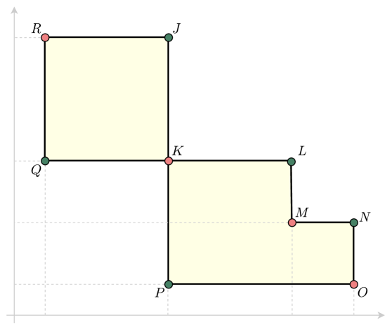
Figure 10.1: An illustration of theorem 10.1.1. The theorem states that given an integrable function $f$, its antiderivative $F\left(x,y\right)\equiv\iint fdx$, and a rectangular domain (highlighted in the above figure), then: $\iint_{D}f(x,y)dxdy=F(J)-2F(K)+F(L)-F(M)+F(N)-F(O)+F(P)+F(Q)-F(R).$ The coefficients of the antiderivative at the corner points are the parameter $\alpha_{D}$ from the formulation of the theorem, and they are uniquely determined according to the corner type.

The derivative sign does not reflect trends at cusp points such as corners; therefore, it does not classify corner types concisely. In contrast, it turns out that the detachment operator classifies corners (and thus defines the parameter $\alpha_{D}$ coherently) independently of the curve’s parameterization; this is a multidimensional generalization of our above discussion regarding the relation between both operators. The theorem utilizes the inclusion-exclusion principle as the series of domains finally add up to the domain bounded by the vertices. While this theorem is defined over continuous domains, it is limited to generalized rectangular ones. Let us attempt to alleviate this limitation.

In the proceeding subsections, we leverage the detachment to define a novel integration method that extends theorem 10.1.1 to non-rectangular domains by combining it with the mean value theorem, as follows. Given a simple closed curve $C$, we will define what it means that it is detachable. Then, let $D$ be the region bounded by the curve. Let $R\subseteq D$ be a rectangular domain circumscribed by $C$. Let ${C_{i}}$ be the sub-curves of $C$ between each pair of its consecutive touching points with $R.$ Let $D_{i}\subset D\backslash R$ be the sub-domain bounded between $C_{i}$ and $R$. Let $\partial D_{i}$ be the boundary of $D_{i}$, and let $\nabla D_{i}$ be the intersection between $D_{i}$ and the vertices of $R$. According to the mean value theorem in two dimensions, $\forall i:\exists x_{i}\in D_{i}$ such that $\underset{{\scriptscriptstyle D_{i}}}{\iint}f\boldsymbol{dx}=\beta_{i}f\left(x_{i}\right)\equiv\boldsymbol{\beta}\cdot\boldsymbol{f\left(x_{\beta}\right)},$ where $\beta_{i}$ is the area of $D_{i}.$

The semi-discrete integration method we will introduce accumulates a linear combination of the function and its antiderivative along the sub-domains $D_{i}$, and yields the following simple result:

Corollary 10.1.2 

Let $D\subset\mathbb{R}^{2}$ be a closed, bounded, and connected domain whose edge is detachable. Let $f:\mathbb{R}^{2}\rightarrow\mathbb{R}$ be a continuous function that admits an antiderivative $F$. Then:

$$\underset{{\scriptscriptstyle D}}{\iint}f\boldsymbol{dx}=\boldsymbol{\alpha}\cdot\boldsymbol{F\left(x_{\alpha}\right)}+\boldsymbol{\beta}\cdot\boldsymbol{f\left(x_{\beta}\right)},$$

where $\boldsymbol{\alpha}\cdot\boldsymbol{F\left(x_{\alpha}\right)}+\boldsymbol{\beta}\cdot\boldsymbol{f\left(x_{\beta}\right)}\equiv\sum\left[\boldsymbol{\alpha_{i}}\cdot F\left(\boldsymbol{x_{\alpha,i}}\right)+\beta_{i}f\left(x_{i}\right)\right]$ and $\boldsymbol{x_{\alpha,i}}=\left(F\left(x\right)\,|\,x\in\nabla D_{i}\right)^{T}$ is the vector of antiderivative values at the vertices of the subdomain $D_{i}$, $\boldsymbol{\alpha_{i}}=\left(\alpha\left(\partial D_{i}^{;},x\right)\,|\,x\in\nabla D_{i}\right)^{T}$ is a vector containing the results of applying a function $\alpha$ to the detachments of the curve $\partial D_{i}^{;}$ at its vertices $\nabla D_{i}$, and $\beta_{i}$ is the area of $D_{i}$, which we incorporate as part of the mean value theorem for integrals along with it matching point in $D_{i}$ denoted by $x_{i}$. The function $\alpha$ is constructed within the integration method based on the curve’s pointwise detachments, as we illustrate in the following subsections.

To establish result 10.1.2 rigorously, let us define the parameter $\alpha_{i}$ with the notion of the curve’s detachment, and introduce an integration method along curves that yields the above result as a relation between the double integral inside the domain and the novel line integral along its boundary, similarly to Green’s theorem.

Figure 10.2: An illustration of corollary 10.1.2. The double integral of a function $f$ defined over the domain equals a sum of two linear combinations: that of the antiderivative $F$ along the inner rectangular domain’s corners (the green and red points, whose coefficients $\boldsymbol{\alpha}$ are determined based on the domain’s detachments), and that of the function $f$ at the interior of the subdomains outside the rectangular domains (the blue points, whose coefficients $\boldsymbol{\beta}$ are determined based on each green subdomain’s area, due to the mean value theorem for integrals in $\mathbb{R}^{2}$).

10.2 Classifying a Curve’s Monotony

For the simplicity of our discussion we focus on $\mathbb{R}^{2}$, and assume that all the curves are continuous, simple, finite, oriented and non oscillating (in a sense that will be clear later). Moreover, we assume that the closed curves are positively oriented, and the domains are simply connected. Having said that, the discussion can be naturally extended to higher dimensions and to curves with more general attributes. Hence, we would like to introduce a tool for classification of corners along a curve, which is a special case of classifying the monotony of the curve. For the sake of coherency and a proper classification, we will require from the classification tool to be dependent of the curve’s spatial representation and orientation, and independent of its parametrization.Let us analyze different parametrizations of the same curve and watch how the derivative yields different results for each of them.

Example 10.2.1 

Let us examine a curve $C$ that consists of two line segments,

$$C:\left(1,0\right)\longrightarrow\left(0,0\right)\longrightarrow\left(0,1\right).$$

Let us evaluate its derivative at the corner point $\left(0,0\right)$ for different parametrizations, determined by the value of a parameter $k>0$:

$$\begin{aligned} &C:\gamma_{k}=\left(x_{k}\left(t\right),y_{k}\left(t\right)\right),\quad 0\leq t\leq 2\\ &\gamma_{k}\left(t\right)=\begin{cases}\left(\left(1-t\right)^{k},0\right),&0\leq t\leq 1\\ \left(0,\left(1-t\right)^{k}\right),&1\leq t\leq 2\end{cases}\end{aligned}$$ (10.1)

• For $k=1$, the curve’s one-sided derivatives are

  $$\partial_{+}x_{1}\left(1\right)=0,\quad\partial_{-}x_{1}\left(1\right)=-1,\quad\partial_{+}y_{1}\left(1\right)=+1\quad\text{and}\quad\partial_{-}y_{1}\left(1\right)=0.$$

• For $k>1$, the curve’s one-sided derivatives are all zeroed at $\left(0,0\right).$

• For $k<1$, the curve’s one-sided derivatives do not exist at $\left(0,0\right)$.

Therefore, the vector $\left(\partial_{+}x,\partial_{-}x,\partial_{+}y,\partial_{-}y\right)\biggm{\lvert}_{t=t_{0}}$ is not a valid tool for the classification of corners (since this vector is dependent of the curve’s parametrization). It should not come to us by surprise, as the derivative is a tool measuring velocity, and the curve’s parametrizations are descriptions of different speeds of movement along the curve.

10.3 Detachments Vector of a Curve

In this subsection, we propose that the vector of the curve’s detachments is a coherent tool for classifying the monotony of a broad set of curves, in the sense that it is independent of the curve’s parametrization.

Definition 10.3.1 — Detachable curve. 

We say that a curve $C$ is detachable at a point $z\in C$ if there is a continuous parametrization $\gamma\left(t\right)=\left(x\left(t\right),y\left(t\right)\right),0\leq t\leq 1$ of $C$ for which $z=\left(x\left(t_{0}\right),y\left(t_{0}\right)\right)$ such that $x,y$ are detachable at $t_{0}$.

We show that in case a curve is detachable at a point, then $x_{\pm}^{;},y_{\pm}^{;}$ are independent of its parametrization. To that end, let us define the following spatial property of the curve.

Definition 10.3.2 — Neighborhood system of a point. 

Given a point $z=\left(x_{0},y_{0}\right)$ in the plane, we define its neighbourhood system as the following eight domains:

$$O_{s_{1},s_{2}}\left(z\right)\equiv\left\{\left(x,y\right)\biggm{\lvert}\text{sgn}\left(x-x_{0}\right)=s_{1},\quad\text{sgn}\left(y-y_{0}\right)=s_{2}\right\}_{s_{1},s_{2}\in\left\{0,\pm 1\right\}},$$

where we omit the degenerated domain $O_{0,0}=\left\{z\right\}$ from the neighborhood system.

Let $z$ be a point on a detachable curve $C$. Assuming $C$ is oriented, we can refer to the set of points on $C$ that are preceding or following $z$ with respect to the orientation. Let us denote those points by $C\bigm{\lvert}_{z^{-}}$ and $C\bigm{\lvert}_{z^{+}}$ respectively.

We claim that $C$ is detachable at $z$ if and only if there is a small enough neighborhood of $z$ such that $C\bigm{\lvert}_{z^{-}}$ and $C\bigm{\lvert}_{z^{+}}$ are each contained in the same domain out of the neighborhood system of $z$. Let us formulate it rigorously. Let $\gamma\left(t\right)=\left(x\left(t\right),y\left(t\right)\right)$ be any continuous parametrization of a detachable curve $C$ such that $\gamma\left(t_{0}\right)=z$. Then:

$$\begin{array}[]{cc}&x_{+}^{;}\left(t_{0}\right)=\delta_{1}\land x_{-}^{;}\left(t_{0}\right)=\delta_{2}\land y_{+}^{;}\left(t_{0}\right)=\delta_{3}\land y_{-}^{;}\left(t_{0}\right)=\delta_{4}\\ \Longleftrightarrow&\begin{cases}\text{sgn}\left[x\left(t_{0}+h\right)-x\left(t_{0}\right)\right]=\delta_{1},&h\rightarrow 0^{+}\\ \text{sgn}\left[x\left(t_{0}\right)-x\left(t_{0}+h\right)\right]=\delta_{2},&h\rightarrow 0^{-}\\ \text{sgn}\left[y\left(t_{0}+h\right)-y\left(t_{0}\right)\right]=\delta_{3},&h\rightarrow 0^{+}\\ \text{sgn}\left[y\left(t_{0}\right)-y\left(t_{0}+h\right)\right]=\delta_{4},&h\rightarrow 0^{-}\end{cases}\\ \Longleftrightarrow&\begin{cases}\exists r^{+}>0:\quad B_{r^{+}}\left(z\right)\bigcap C\bigm{\lvert}_{z^{+}}\subseteq O_{\delta_{1},\delta_{3}}\left(z\right)\\ \exists r^{-}>0:\quad B_{r^{-}}\left(z\right)\bigcap C\bigm{\lvert}_{z^{-}}\subseteq O_{\delta_{2},\delta_{4}}\left(z\right).\end{cases}\end{array}$$

Since condition 10.3 is independent of the curve’s parametrization, we conclude that so is the vector $\left\{\delta_{i}\right\}_{1\leq i\leq 4}$. Hence the following definition.

Definition 10.3.3 — Detachments vector of a detachable curve. 

Suppose that a curve $C$ is detachable at $z\in C$. We define the curve’s detachments vector at $z$ as:

$$\delta C\left(z\right)\equiv\left(x_{+}^{;},x_{-}^{;},y_{+}^{;},y_{-}^{;}\right)\biggm{\lvert}_{t_{0}},$$

where $\left(x\left(t\right),y\left(t\right)\right)$ is any continuous parametrization of $C$ for which $z=\left(x\left(t_{0}\right),y\left(t_{0}\right)\right)$.

In the following discussion we omit the notion of the curve’s parametrization whenever possible, since a curve’s detachments vector is independent of its parametrization.

Let $C$ be a curve, and let $z$ be a point on $C$. Then:

1. If $C$ admits a constant detachments vector in the neighbordhood of $z$, then $\delta C\left(z\right)$ is one of the following values:

   $$\begin{aligned} &\left\{\left(-1,+1,0,0\right),\left(0,0,+1,-1\right),\left(+1,-1,+1,-1\right),\left(+1,-1,-1,+1\right)\right\}\\ \bigcup&\left\{\left(-1,+1,-1,+1\right),\left(-1,+1,+1,-1\right),\left(+1,-1,0,0\right),\left(0,0,-1,+1\right)\right\}\end{aligned}$$ (10.2)

2. If $z$ is a right corner then $\delta C\left(z\right)$ accepts one of the following values:

   $$\begin{aligned} &\left\{\left(+1,0,0,-1\right),\left(-1,0,0,-1\right),\left(0,-1,+1,0\right),\left(0,+1,+1,0\right)\right\}\\ \bigcup&\left\{\left(0,+1,-1,0\right),\left(0,-1,-1,0\right),\left(-1,0,0,+1\right),\left(+1,0,0,+1\right)\right\}\end{aligned}$$ (10.3)

10.4 A Curve’s Detachment

In this subsection we introduce an attribute of a curve at a point, namely its detachment, which is determined according to the detachment vector, or equivalently, according to the domains (out of the point’s neighborhood system) in which the curve resides close to the point. A possible geometric interpretation of the curve’s detachment at a point $z\in C$ is the sign of the sum of

$$\alpha_{O_{s_{1},s_{2}}^{\pm}\left(z\right)},$$

where $O_{s_{1},s_{2}}^{\pm}\left(z\right)$ are the domains (out of the point’s neighborhood system) that reside left to the curve in $C\bigm{\lvert}_{z^{\pm}}$ respectively, and $\alpha_{D}$ is determined as in theorem 10.1.1. This definition extends the parameter $\alpha_{D}$, in the sense that it coalesces with it at the right corners. The geometric interpretation of a curve’s detachment will become clearer once we apply it to extend that theorem to more general domains in subsection 10.5, to obtain a rigorous version of corollary 10.1.2 above.

We extract definition 10.4.1 by reverse engineering the possible values of the curve’s detachment given this geometric interpretation.

Definition 10.4.1 — Detachment of a curve. 

Let $C$ be a detachable curve. We define the detachment of the curve $C$ at the point $z\in C$ as a function of its detachments vector $\delta C\left(z\right)=\left(x^{;}_{+},x^{;}_{-},y^{;}_{+},y^{;}_{-}\right)$ as follows:

$$C^{;}\left(z\right)\equiv y_{-}^{;}\text{sgn}\left(y_{-}^{;}-x_{-}^{;}\right)-y_{+}^{;}\text{sgn}\left(y_{+}^{;}+x_{+}^{;}\right).$$

See the exact values in table 10.1. We will clarify this closed algebraic formula for the detachment via its geometric meaning in the below discussion.

$\boldsymbol{x_{+}^{;}}$	$\boldsymbol{x_{-}^{;}}$	$\boldsymbol{y_{+}^{;}}$	$\boldsymbol{y_{-}^{;}}$
$+1$	$-1$	$+1$	$-1$
$-1$	$+1$	$-1$	$+1$
$0$	$-1$	$-1$	$0$
$0$	$+1$	$+1$	$0$
$0$	$-1$	$+1$	$0$
$0$	$+1$	$-1$	$0$
$0$	$+1$	$+1$	$+1$
$-1$	$-1$	$-1$	$0$
$+1$	$+1$	$+1$	$0$
$0$	$-1$	$-1$	$-1$
$-1$	$+1$	$-1$	$0$
$0$	$+1$	$-1$	$+1$
$0$	$-1$	$+1$	$-1$
$+1$	$-1$	$+1$	$0$
$+1$	$+1$	$+1$	$+1$
$-1$	$-1$	$-1$	$-1$

$\boldsymbol{x_{+}^{;}}$	$\boldsymbol{x_{-}^{;}}$	$\boldsymbol{y_{+}^{;}}$	$\boldsymbol{y_{-}^{;}}$
$-1$	$-1$	$-1$	$+1$
$+1$	$+1$	$-1$	$+1$
$+1$	$-1$	$-1$	$-1$
$+1$	$-1$	$+1$	$+1$
$+1$	$+1$	$+1$	$-1$
$-1$	$-1$	$+1$	$-1$
$-1$	$+1$	$-1$	$-1$
$-1$	$+1$	$+1$	$+1$
$0$	$-1$	$+1$	$+1$
$-1$	$0$	$-1$	$-1$
$+1$	$+1$	$0$	$+1$
$-1$	$-1$	$+1$	$0$
$+1$	$+1$	$-1$	$0$
$-1$	$-1$	$0$	$-1$
$+1$	$0$	$+1$	$+1$
$0$	$+1$	$-1$	$-1$
$-1$	$+1$	$+1$	$0$
$-1$	$+1$	$0$	$+1$
$0$	$-1$	$-1$	$+1$
$-1$	$0$	$-1$	$+1$
$+1$	$0$	$+1$	$-1$
$0$	$+1$	$+1$	$-1$
$+1$	$-1$	$0$	$-1$
$+1$	$-1$	$-1$	$0$
$+1$	$+1$	$0$	$0$
$-1$	$-1$	$0$	$0$
$0$	$0$	$-1$	$-1$
$0$	$0$	$+1$	$+1$

$\boldsymbol{x_{+}^{;}}$	$\boldsymbol{x_{-}^{;}}$	$\boldsymbol{y_{+}^{;}}$	$\boldsymbol{y_{-}^{;}}$
$+1$	$-1$	$-1$	$+1$
$-1$	$+1$	$+1$	$-1$
$+1$	$0$	$0$	$-1$
$-1$	$0$	$0$	$+1$
$+1$	$0$	$0$	$+1$
$-1$	$0$	$0$	$-1$
$+1$	$0$	$0$	$-1$
$+1$	$+1$	$0$	$-1$
$-1$	$-1$	$0$	$+1$
$-1$	$0$	$+1$	$+1$
$-1$	$+1$	$0$	$-1$
$+1$	$0$	$-1$	$+1$
$-1$	$0$	$+1$	$-1$
$+1$	$-1$	$0$	$+1$
$+1$	$+1$	$-1$	$-1$
$-1$	$-1$	$+1$	$+1$

Table 10.1: Tables defining the term $C^{;}$ from definition 10.4.1. The left, middle and right tables correspond to detachment vectors yielding $C^{;}$ of $-1,0$ and $+1$, respectively.

10.5 Defining the Semi-discrete Line Integral

In this subsection we introduce an integration method whose aim is to naturally extend theorem 10.1.1 to non-rectangular domains, as in corollary 10.1.2. In 10.5.5 we define the integration method for monotonic curves, in subsection 10.5.2 we formulate some of its algebraic properties, and in subsection 10.5.3 we extend the integration method to general curves and deduce corollary 10.1.2.

10.5.1 Defining the Semi-discrete Line Integral for Monotonic Curves

Definition 10.5.1 — Monotonic curve. 

We say that a curve is monotonic if its detachments vector is constant, except, perhaps, at its endpoints. The detachment of a monotonic curve is defined as its (constant) detachment at internal points.

Corollary 10.5.1 

Let $C$ be a monotonic curve. Then $C$ is entirely contained in a (possibly degenerated) rectangle whose opposite vertices are the endpoints of $C$.

Proof.

Let $\gamma\left(t\right)=\left(x\left(t\right),y\left(t\right)\right),\quad 0\leq t\leq 1$ be any continuous parametrization of $C.$ According to remark 10.3 combined with lemma 9.4.4, both the functions $x$ and $y$ are strictly monotonous. Without loss of generality, let us analyze two possible values of the curve’s constant detachments vector $\delta\left(C\right).$ In case $\delta\left(C\right)=\left(+1,-1,+1,-1\right)$, then for each $0<t<1$, it holds that $x\left(0\right)<x\left(t\right)<x\left(1\right)$ and $y\left(0\right)<y\left(t\right)<y\left(1\right),$ hence the curve’s points are fully contained in the square $\left[x\left(0\right),y\left(0\right)\right]\times\left[x\left(1\right),y\left(1\right)\right].$ In case $\delta\left(C\right)=\left(-1,+1,0,0\right)$, then for each $0<t<1$, it holds that $x\left(1\right)<x\left(t\right)<x\left(0\right)$ and $y\left(0\right)=y\left(t\right)=y\left(1\right),$ and the statement holds. ∎

Definition 10.5.2 — Straight path of a pair of points. 

Given a pair of points,

$$\left\{x=\left(a,b\right),y=\left(c,d\right)\right\}\subset\mathbb{R}^{2},$$

we define the following paths:

$$\begin{aligned} &\gamma^{+}\left(x,y\right):&\left(a,b\right)\longrightarrow\left(a,d\right)\longrightarrow\left(c,d\right)\\ &\gamma^{-}\left(x,y\right):&\left(a,b\right)\longrightarrow\left(c,b\right)\longrightarrow\left(c,d\right)\end{aligned}$$ (10.4)

as the positive and negative straight paths of $\left\{x,y\right\}$, respectively. We denote the mentioned points along the paths as follows:

$$\gamma_{1}\left(x,y\right)=\left(a,b\right),\quad\gamma^{+}_{2}\left(x,y\right)=\left(a,d\right),\quad\gamma^{-}_{2}\left(x,y\right)=\left(c,b\right),\quad\gamma_{3}\left(x,y\right)=\left(c,d\right).$$

If we omit the sign subscript, then a positive sign is assumed, for example $\gamma\left(x,y\right)\equiv\gamma^{+}\left(x,y\right)$ and $\gamma_{2}\left(x,y\right)\equiv\gamma^{+}_{2}\left(x,y\right).$

Definition 10.5.3 — Paths of a curve. 

Let $C$ be a given monotonic curve with endpoints $\left\{z_{0},z_{1}\right\}.$ We define the curve’s positive and negative paths,denoted by $C^{\pm}$, respectively, as the straight paths between the endpoints:

$$C^{\pm}\equiv\gamma^{\pm}\left(z_{0},z_{1}\right).$$

We denote the points along the curve’s paths by $C_{i}^{\pm}\left(z_{0},z_{1}\right)=\gamma_{i}^{\pm}\left(z_{0},z_{1}\right)$ (see definition 10.5.2 above). If we omit the sign subscript, then a positive sign is assumed. Thus, $C_{i}\equiv C^{+}_{i}.$

Definition 10.5.4 — Local domains. 

Given a monotonic curve $C$, we define the positive and negative local domains of $C$, namely $D^{\pm}\left(C\right)$, as the closed domains whose boundaries satisfy:

$$\partial D^{\pm}\left(C\right)\equiv C^{\pm},$$

where $C^{\pm}$ are the positive and negative paths of $C$, respectively. If we omit the sign subscript then a positive sign is assumed. Thus, $D\left(C\right)\equiv D^{+}\left(C\right).$

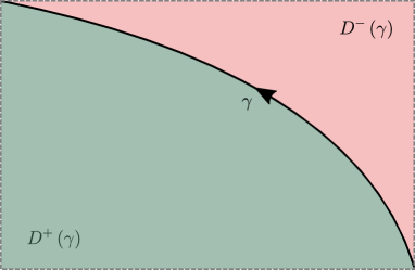
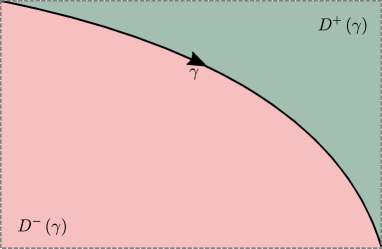
Positively oriented curve	Negatively oriented curve

Figure 10.3: Local domains of a monotonic curve. The positive domain is the left hand-side of the curve that is bounded by its positive straight path. Note that as the curve’s orientation flips, so do the signs of the local domains.

A monotonic curve’s local domains may be degenerated in case some entries of the curve’s detachments vector are zeroed.

Definition 10.5.5 — Semi-discrete line integral over a monotonic curve. 

Let $C\subset\mathbb{R}^{2}$ be a curve, and let $\ell\subset C$ be a monotonic subcurve of $C$, whose constant detachment is $\ell^{;}$. Let us consider a function $f:\mathbb{R}^{2}\rightarrow\mathbb{R}$ that admits an antiderivative $F$. We define the semi-discrete line integral of $F$ along the curve $\ell$ in the context of the curve $C$ as follows:

$$\underset{\ell\subset C}{\sqint}F\equiv\underset{D\left(\ell\right)}{\iint}f\boldsymbol{dx}-\ell^{;}F\left(\ell_{2}\right)+\frac{1}{2}\left[\ell_{1}^{;}F\left(\ell_{1}\right)+\ell_{3}^{;}F\left(\ell_{3}\right)\right],$$

where $\ell_{i}^{;}=C^{;}\left(\ell_{i}\right)$. If the context $C$ is clear, then we denote the term $\underset{\ell\subset C}{\sqint}F$ as $\underset{\ell}{\sqint}F$.

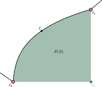
Figure 10.4: An illustration of the definition of the semi-discrete line integral over a monotonic curve. In this example, the curve $C$ has a highlighted subcurve, denoted by $\ell$. The detachments vector of $\ell$ is constant ($\delta\ell=\left(-1,+1,-1,+1\right)$), and its detachment is $\ell^{;}=-1$. The detachment at the subcurve’s endpoints is $\ell_{1}^{;}=-1$ and $\ell_{3}^{;}=-1$ for the point $\ell_{1}$ and $\ell_{3}$, respectively. Hence, according to the definition: $\underset{\ell}{\sqintop}F=\underset{D\left(\ell\right)}{\iint}fdx+F\left(\ell_{2}\right)-\frac{1}{2}\left[F\left(\ell_{1}\right)+F\left(\ell_{3}\right)\right].$

10.5.2 Algebraic Properties of the Semi-discrete Line Integral

We show that the semi-discrete line integral is a linear operator in the following sense.

Claim 10.5.1 

Constant multiplication rule. Let $c\in\mathbb{R}$ and $F$ be an antiderivative defined over the detachable curve $\ell\subset C$. Then:

$$\underset{\ell}{\sqint}\left(cF\right)=c\underset{\ell}{\sqint}F.$$

Proof.

From the linearity of the double integral, if the antiderivative of $f$ is $F$, then the antiderivative of $cf$ is $cF$. Then:

$$\begin{aligned} \underset{\ell}{\sqint}\left(cF\right)&\equiv\underset{D\left(\ell\right)}{\iint}\left(cf\right)\boldsymbol{dx}-\ell^{;}\left(cF\right)\left(\ell_{2}\right)+\frac{1}{2}\left[\ell_{1}^{;}\left(cF\right)\left(\ell_{1}\right)+\ell_{3}^{;}\left(cF\right)\left(\ell_{3}\right)\right]\\ &=c\underset{D\left(\ell\right)}{\iint}f\boldsymbol{dx}-c\ell^{;}F\left(\ell_{2}\right)+\frac{1}{2}\left[c\ell_{1}^{;}F\left(\ell_{1}\right)+c\ell_{3}^{;}F\left(\ell_{3}\right)\right]\\ &=c\left\{\underset{D\left(\ell\right)}{\iint}f\boldsymbol{dx}-\ell^{;}F\left(\ell_{2}\right)+\frac{1}{2}\left[\ell_{1}^{;}F\left(\ell_{1}\right)+\ell_{3}^{;}F\left(\ell_{3}\right)\right]\right\}\equiv c\underset{\ell}{\sqint}F.\end{aligned}$$ (10.5)

∎

Lemma 10.5.2 

Let $C$ be a curve, and let $\alpha,\beta$ be monotonic subcurves of $C$ such that $\alpha\bigcup\beta$ is monotonic and continuous. Let $f:\mathbb{R}^{2}\rightarrow\mathbb{R}$ be a function that admits an antiderivative $F$. Then:

$$\underset{\alpha\bigcup\beta}{\sqint}F=\underset{\alpha}{\sqint}F+\underset{\beta}{\sqint}F$$

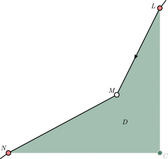
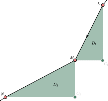
Semi-discrete line integral on $LMN$	Semi-discrete line integrals on $LM$, $MN$

Figure 10.5: An illustration of the proof of lemma 10.5.2. On the right: the semi-discrete line integral over the curve $LMN$ is $\underset{LMN}{\sqint}F\equiv\underset{D}{\iint}f\left(x,y\right)dxdy+F\left(C\right)-\frac{1}{2}\left[F\left(L\right)+F\left(N\right)\right].$ On the left: the semi-discrete line integral over $LM$ is $\underset{LM}{\sqint}F\equiv\underset{D_{1}}{\iint}f\left(x,y\right)dxdy+F\left(C_{1}\right)-\frac{1}{2}\left[F\left(L\right)+F\left(M\right)\right]$, and that over $MN$ is $\underset{MN}{\sqint}F\equiv\underset{D_{2}}{\iint}f\left(x,y\right)dxdy+F\left(C_{2}\right)-\frac{1}{2}\left[F\left(M\right)+F\left(N\right)\right]$. Hence by applying theorem \wang to the rectangular domain $MC_{1}CC_{2}$, we obtain $\underset{LM}{\sqintop}F+\underset{MN}{\sqintop}F=\underset{LMN}{\sqintop}F.$

Proof.

For the sake of convenience, let us denote $\gamma=\alpha\bigcup\beta.$ Let us assume that $\alpha\bigcap\beta=\left\{\alpha_{3}\right\}=\left\{\beta_{1}\right\}$ and that $\gamma_{1}=\alpha_{1},\quad\gamma_{3}=\beta_{3}.$ Since $\delta\left(\alpha\right)=\delta\left(\beta\right)=\delta\left(\gamma\right),$ then the curves also share a constant detachment $\gamma^{;}$. According to definition 10.5.5, we have:

$$\begin{aligned} \underset{\alpha}{\fint}F&\equiv\underset{D\left(\alpha\right)}{\iint}f\boldsymbol{dx}-\gamma^{;}F\left(\alpha_{2}\right)+\frac{1}{2}\left[\alpha_{1}^{;}F\left(\alpha_{1}\right)+\alpha_{3}^{;}F\left(\alpha_{3}\right)\right]\\ \underset{\beta}{\fint}F&\equiv\underset{D\left(\beta\right)}{\iint}f\boldsymbol{dx}-\gamma^{;}F\left(\beta_{2}\right)+\frac{1}{2}\left[\alpha_{3}^{;}F\left(\alpha_{3}\right)+\beta_{3}^{;}F\left(\beta_{3}\right)\right]\\ \underset{\gamma}{\fint}F&\equiv\underset{D\left(\gamma\right)}{\iint}f\boldsymbol{dx}-\gamma^{;}F\left(\gamma_{2}\right)+\frac{1}{2}\left[\alpha_{1}^{;}F\left(\alpha_{1}\right)+\beta_{3}^{;}F\left(\beta_{3}\right)\right].\end{aligned}$$ (10.6)

Applying theorem 10.1.1 to the rectangle $\alpha_{2}\alpha_{3}\beta_{2}\gamma_{2}$ results with:

$$\underset{D\left(\gamma\right)}{\iint}f\boldsymbol{dx}\equiv\underset{D\left(\alpha\right)}{\iint}f\boldsymbol{dx}+\underset{D\left(\beta\right)}{\iint}f\boldsymbol{dx}+\gamma^{;}\left\{\left[F\left(\alpha_{2}\right)+F\left(\beta_{2}\right)\right]-\left[F\left(\alpha_{3}\right)+F\left(\gamma_{2}\right)\right]\right\},$$

and by inspecting all the possible values for $\alpha_{1}^{;},\alpha_{3}^{;},\beta_{3}^{;}$ and $\gamma^{;}$, we conclude the statement’s correctness. ∎

Corollary 10.5.2 

Let $C$ be a detachable curve and let $\ell$ be a monotonic subcurve of $C$ whose detachment is $\ell^{;}$. Denote by $-\ell$ and $-C$ the curves $\ell$ and $C$ with flipped orientations, respectively. Suppose that the detachments along the curves $\pm\ell$ are nowhere zeroed, not even at their endpoints $\ell_{1},\ell_{3}$. Let $f:\mathbb{R}^{2}\rightarrow\mathbb{R}$ be a function that admits an antiderivative $F$. Then it holds that:

$$\underset{-\ell\subset-C}{\sqint}F=-\underset{\ell\subset C}{\sqint}F.$$

Proof.

Applying theorem 10.1.1 to the rectangle whose boundary is $\ell_{1}\ell_{2}^{+}\ell_{3}\ell_{2}^{-}$ results with:

$$\underset{D^{+}\left(\ell\right)}{\iint}f\boldsymbol{dx}+\underset{D^{-}\left(\ell\right)}{\iint}f\boldsymbol{dx}=\ell^{;}\left\{F\left(\ell_{1}\right)+F\left(\ell_{3}\right)-\left[F\left(\ell_{2}^{+}\right)+F\left(\ell_{2}^{-}\right)\right]\right\}.$$

The corollary follows by combining equation 10.5.2 with the definitions of $\underset{\pm\ell\subset\pm C}{\sqint}F,$ while considering all the cases of $\ell^{;}$ and $\delta\left(\ell\right)\bigm{\lvert}_{\ell_{1},\ell_{3}}$, rearranging the terms and applying the definition of the semi-discrete line integral for $\ell$. ∎

Corollary 10.5.3 

Let $\ell$ be a monotonic curve such that $\ell^{;}\equiv 0$, also at the curve’s endpoints $\ell_{1},\ell_{3}$. Then for any function $F$ it holds that $\underset{\ell}{\sqint}F=0.$

Proof.

According to remark 10.3, and since the curve’s detachment is zeroed, the curve’s detachments vector satisfies:

$$\delta\left(\ell\right)\in\left\{\left(+1,-1,0,0\right),\left(-1,+1,0,0\right),\left(0,0,+1,-1\right),\left(0,0,-1,+1\right)\right\}.$$

Thus, the (positive) local domain of $\ell$ is degenerated; hence, the integral over it is zeroed. Furthermore, all the terms that involve the detachment at the definition of the semi-discrete line integral are zeroed as well. Hence, the semi-discrete line integral of any function along $\ell$ is zeroed. ∎

10.5.3 Defining the Semi-discrete Line Integral for General Curves

Let us extend the definition of the semi-discrete line integral over monotonic curves to unions of such curves.

Definition 10.5.6 — Monotonic division of a curve. 

Let $C$ be a detachable curve in $\mathbb{R}^{2}$. A monotonic division of $C$ is an ordered set of subcurves $\left\{\ell_{i}\right\}_{1\leq i\leq n}$, such that each $\ell_{i}$ is a monotonic subcurve of $C$ whose detachment $\ell_{i}^{;}$ is constant, and:

$$C=\bigcup_{i=1}^{n}\ell_{i}.$$

Definition 10.5.6 is illustrated in Figure 10.6.

Definition 10.5.7 — Discrete line integral over a detachable curve. 

Let $C$ be a detachable curve, and let $\left\{\ell_{i}\right\}_{1\leq i\leq n}$ be a monotonic division of a subcurve $\ell\subset C$. Let us consider a function $f:\mathbb{R}^{2}\rightarrow\mathbb{R}$ that admits an antiderivative $F$. Then the semi-discrete line integral of $F$ over $\ell$ in the context of the curve $C$ is defined as follows:

$$\underset{\ell\subset C}{\sqint}F\equiv\underset{i}{\sum}\underset{\ell_{i}\subset C}{\sqint}F,$$

where each $\underset{\ell_{i}\subset C}{\sqint}F$ is calculated according to the definition of the semi-discrete line integral over monotonic curves, as in definition 10.5.5.

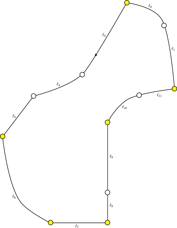
Figure 10.6: An illustration of a monotonic division of a detachable curve. The points defining the curve’s mininal division are highlighted. The empty points are not part of the mininal division, in the sense that we may coalesce the following curves and remain with a monotonic division (since their detachments vectors are equal): $\ell_{1}$ with $\ell_{2}$; $\ell_{3}$ with $\ell_{4}$ and $ell_{5}$; $ell_{8}$ with $\ell_{9}$; and $\ell_{10}$ with $\ell_{11}$. We illustrate the semi-discrete line integral along one of the induced monotonic divisions in figure 10.7.

Note that the notion of semi-discrete line integral over a detachable curve is well-defined because the right hand-side is independent of the curve’s division, due to the additivity of the semi-discrete line integral over monotonic curves (lemma 10.5.2).

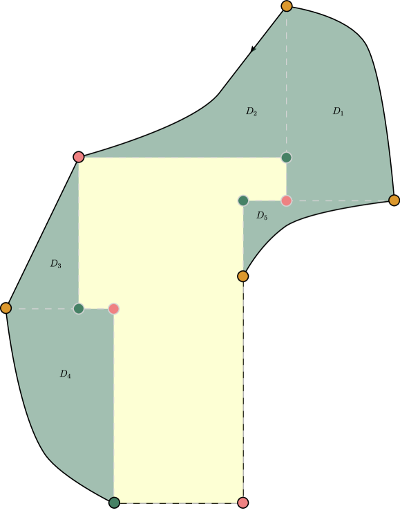
Figure 10.7: An illustration of the semi-discrete line integral applied to each segment of a monotonic division of the detachable curve from figure 10.6. The $D_{1}=D^{+}\left(\ell_{1}\bigcup\ell_{2}\right)$, $D_{2}=D^{+}\left(\ell_{3}\bigcup\ell_{4}\right)$, $D_{3}=D^{+}\left(\ell_{5}\right)$, $D_{4}=D^{+}\left(\ell_{6}\right)$ and $D_{5}=D^{+}\left(\ell_{10}\bigcup\ell_{11}\right)$ are the positive domains of the curve’s respective subsegments.

10.6 Establishing a Semi-discrete Version of Green’s Theorem

In this section we apply the definition of the semi-discrete line integral to extend theorem 10.1.1 to general domains rather than merely rectangular ones, as in corollary 10.1.2. We already saw the final result in corollary 10.1.2, and we will aim to arrive at that formula via the definition of the integral, to obtain a semi-discrete version of Green’s theorem. We begin by formulating the following lemma.

Lemma 10.6.1 

Let $\left\{\ell_{i}\right\}_{1\leq i\leq n}$ be a monotonic division of a closed and detachable curve $\gamma$. Let $f:\mathbb{R}^{2}\rightarrow\mathbb{R}$ be a function that admits an antiderivative $F$. Let $M,N,O$ be the endpoints of the curves $\ell_{1},\ell_{2}$ respectively (where $M=\ell_{1}\bigcap\ell_{2}$). Let:

$$\alpha\equiv\ell_{1}\bigcup\ell_{2}\bigcup\overrightarrow{MO},$$

and:

$$\beta\equiv\bigcup_{i=1}^{n}\ell_{i}\bigcup\overrightarrow{OM}.$$

Then:

$$\underset{\gamma}{\sqint}F=\underset{\alpha}{\sqint}F+\underset{\beta}{\sqint}F.$$

Proof.

. We know that $\underset{\gamma}{\sqint}F-\underset{\beta}{\sqint}F-\underset{\alpha}{\sqint}F=0.$ Let us evaluate these terms:

$$\begin{aligned} \underset{\alpha}{\sqint}F&=\underset{\ell_{1}\subset\alpha}{\sqint}F+\underset{\ell_{2}\subset\alpha}{\sqint}F+\underset{\overrightarrow{MO}\subset\alpha}{\sqint}F,\\ \underset{\beta}{\sqint}F&=\underset{\overrightarrow{OM}\subset\alpha}{\sqint}F+\underset{\ell_{3}\subset\beta}{\sqint}F+\underset{\bigcup_{i=4}^{n-1}\ell_{i}\subset\beta}{\sqint}F+\underset{\ell_{n}\subset\beta}{\sqint}F,\\ \underset{\gamma}{\sqint}F&=\underset{\ell_{1}\subset\gamma}{\sqint}F+\underset{\ell_{2}\subset\gamma}{\sqint}F+\underset{\ell_{3}\subset\gamma}{\sqint}F+\underset{\bigcup_{i=4}^{n-1}\ell_{i}\subset\gamma}{\sqint}F+\underset{\ell_{n}\subset\gamma}{\sqint}F.\end{aligned}$$ (10.7)

For readability and without loss of generality, let us assume that $\gamma$ is structured as depicted in Figure 10.6.1.

By definition, the semi-discrete line integral of $F$ over $\ell_{1}$ in the context of the curve $\gamma$ equals:

$$\underset{\ell_{1}\subset\gamma}{\sqint}F=\underset{D\left(\ell_{1}\right)}{\iint}f\boldsymbol{dx}-\ell_{1}^{;}F\left(O^{\prime}\right)+\frac{1}{2}\left[\gamma^{;}\left(N\right)F\left(N\right)+\gamma^{;}\left(O\right)F\left(O\right)\right],$$

where $\ell_{1}^{;}$ is the detachment of the monotonic curve $\ell_{1}$, and $\gamma^{;}\left(N\right),\gamma^{;}\left(O\right)$ are the detachments of the points $N$ and $O$ in the context of the curve $\gamma$, respectively.

Similarly, the discrete line integral of $F$ over $\ell_{1}$ in the context of the curve $\alpha$ is:

$$\underset{\ell_{1}\subset\alpha}{\sqint}F=\underset{D\left(\ell_{1}\right)}{\iint}f\boldsymbol{dx}-\ell_{1}^{;}F\left(O^{\prime}\right)+\frac{1}{2}\left[\alpha^{;}\left(N\right)F\left(N\right)+\alpha^{;}\left(O\right)F\left(O\right)\right],$$

where $\alpha^{;}\left(N\right),\alpha^{;}\left(O\right)$ are the detachments at the points $N$ and $O$ in the context of the curve $\alpha$, respectively.

Hence:

$$\underset{\ell_{1}\subset\gamma}{\sqint}F-\underset{\ell_{1}\subset\alpha}{\sqint}F=\frac{1}{2}\left[\gamma^{;}\left(O\right)-\alpha^{;}\left(O\right)\right]F\left(O\right)=\frac{1}{2}\left(+1-0\right)F\left(O\right)=\frac{1}{2}F\left(O\right).$$

Similarly:

$$\begin{aligned} \underset{\ell_{1}\subset\gamma}{\sqint}F-\underset{\ell_{2}\subset\alpha}{\sqint}F&=\frac{1}{2}\left[\gamma^{;}\left(M\right)-\alpha^{;}\left(M\right)\right]F\left(M\right)=\frac{1}{2}\left[-1-\left(-1\right)\right]F\left(M\right)=0,\\ \underset{\bigcup_{i=4}^{n-1}\ell_{i}\subset\gamma}{\sqint}F-\underset{\bigcup_{i=4}^{n-1}\ell_{i}\subset\beta}{\sqint}F&=0,\\ \underset{\ell_{3}\subset\gamma}{\sqint}F-\underset{\ell_{3}\subset\beta}{\sqint}F&=\frac{1}{2}\left[\gamma^{;}\left(M\right)-\beta^{;}\left(M\right)\right]F\left(M\right)=\frac{1}{2}\left[-1-\left(-1\right)\right]F\left(M\right)=0\\ \underset{\ell_{n}\subset\gamma}{\sqint}F-\underset{\ell_{n}\subset\alpha}{\sqint}F&=\frac{1}{2}\left[\gamma^{;}\left(O\right)-\beta^{;}\left(O\right)\right]F\left(O\right)=\frac{1}{2}\left[+1-0\right]F\left(O\right)=0.\end{aligned}$$ (10.8)

Thus, upon placing these values in equations 10.7, we have:

$$\underset{\gamma}{\sqint}F-\underset{\beta}{\sqint}F-\underset{\alpha}{\sqint}F=F\left(O\right)-\left(\underset{\overrightarrow{OM}\subset\beta}{\sqint}F+\underset{\overrightarrow{MO}\subset\alpha}{\sqint}F\right).$$

Once again, according to the definition of the semi-discrete line integral:

$$\begin{aligned} \underset{\overrightarrow{OM}\subset\beta}{\sqint}F&=\underset{OMM^{\prime\prime}}{\iint}f\boldsymbol{dx}-\left(\overrightarrow{OM}\right)^{;}F\left(M^{\prime\prime}\right)+\frac{1}{2}\left[\beta^{;}\left(O\right)F\left(O\right)+\beta^{;}\left(M\right)F\left(M\right)\right],\\ \underset{\overrightarrow{MO}\subset\alpha}{\sqint}F&=\underset{OMM^{\prime\prime}}{\iint}f\boldsymbol{dx}-\left(\overrightarrow{MO}\right)^{;}F\left(M^{\prime}\right)+\frac{1}{2}\left[\alpha^{;}\left(O\right)F\left(O\right)+\alpha^{;}\left(M\right)F\left(M\right)\right].\end{aligned}$$ (10.9)

Hence:

$$\underset{\overrightarrow{OM}\subset\beta}{\sqint}F+\underset{\overrightarrow{MO}\subset\alpha}{\sqint}F=\underset{OM^{\prime}MM^{\prime\prime}}{\iint}f\boldsymbol{dx}+F\left(M^{\prime}\right)+F\left(M^{\prime\prime}\right)-F\left(M\right).$$

Placing this result in equation 10.6 yields:

$$\underset{\gamma}{\sqint}F-\underset{\beta}{\sqint}F-\underset{\alpha}{\sqint}F=F\left(O\right)-F\left(M^{\prime}\right)-F\left(M^{\prime\prime}\right)+F\left(M\right)-\underset{OM^{\prime}MM^{\prime\prime}}{\iint}f\boldsymbol{dx}=0,$$

where the last transition is due to theorem 10.1.1. This shows that, under our assumption, $\underset{\gamma}{\sqint}F=\underset{\alpha}{\sqint}F+\underset{\beta}{\sqint}F$, and we are done.

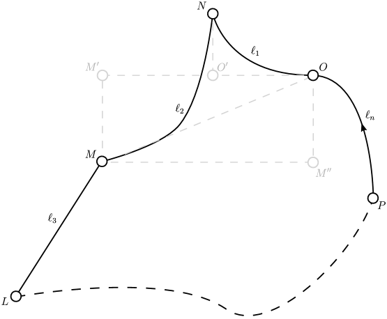
Figure 10.8: An illustration of the proof of lemma 10.6.1

We made the following assumptions throughout the proof:

$$\gamma^{;}\left(O\right)=+1,\quad\gamma^{;}\left(M\right)=-1,\quad\delta\ell_{1}=\left(-1,+1,+1,-1\right),\quad\delta\ell_{2}=\left(-1,+1,-1,+1\right).$$

Other cases left to be handled are different versions of the curve $\gamma$, that vary for different values of $\delta\ell_{1},\delta\ell_{2}$ (each accepts only a few values according to corollary 10.5.1) and $\gamma^{;}\left(M\right),\gamma^{;}\left(O\right)$. There are $\frac{8^{2}\cdot 3^{2}}{4}=144$ different cases, where the division is due to symmetry-induced redundancy. The proof is complete by a computerized inspection of the other cases which is similar to the analysis we introduced. ∎

Now, we may formulate the extension of theorem 10.1.1 in $\mathbb{R}^{2}$ that relies on the definition of the semi-discrete line integral. Let us get inspired by the formulation of Green’s theorem:

Theorem 10.6.1 — Green’s theorem. 

Let $C$ be a positively oriented, piecewise smooth, simple closed curve in a plane, and let $D$ be the region bounded by $C$. If $L$ and $M$ are functions of $\left(x,y\right)$ defined on an open region containing $D$ and having continuous partial derivatives, then

$$\underset{C}{\ointctrclockwise}{\displaystyle\left(L\,dx+M\,dy\right)}{\displaystyle=\underset{D}{\iint}\left(\frac{\partial M}{\partial x}-\frac{\partial L}{\partial y}\right)dx\,dy},$$

where the path of integration along $C$ is anticlockwise.

Let us suggest the following semi-discrete line integral-based analogue to Green’s theorem.

Theorem 10.6.2 — A semi-discrete Green’s theorem. 

Let $D\subset\mathbb{R}^{2}$ be a domain whose edge is detachable. Let $f:\mathbb{R}\rightarrow\mathbb{R}$ be a function that admits an antiderivative $F$. Then:

$$\underset{D}{\iint}f\boldsymbol{dx}=\underset{\partial D}{\sqint}F.$$

Proof.

Let $\left\{\ell_{i}\right\}_{1\leq i\leq n}$ be the minimal monotonic division of $\partial D$. Let us suggest a proof by induction on $n$. The case where $n=1$ is degenerated.

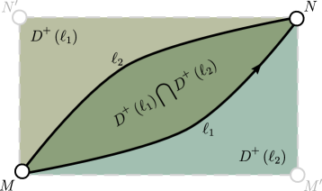
Figure 10.9: An illustration of the proof of theorem 10.6.2 for $n=2$, where the domain’s edge is $\ell_{1}\bigcup\ell_{2}$.

For $n=2$, without loss of generality let us assume the case illustrated in figure 10.9. We have that:

$$\underset{\ell_{1}}{\sqint}F =\underset{D\left(\ell_{1}\right)}{\iint}f\boldsymbol{dx}-\ell_{1}^{;}F\left(N^{\prime}\right)+\frac{1}{2}\left[\gamma^{;}\left(M\right)F\left(M\right)+\gamma^{;}\left(N\right)F\left(N\right)\right],$$

$$\underset{\ell_{2}}{\sqint}F =\underset{D\left(\ell_{2}\right)}{\iint}f\boldsymbol{dx}-\ell_{2}^{;}F\left(M^{\prime}\right)+\frac{1}{2}\left[\gamma^{;}\left(M\right)F\left(M\right)+\gamma^{;}\left(N\right)F\left(N\right)\right].$$

Hence, in the illustrated case, we have that:

$$\underset{D}{\iint}f\boldsymbol{dx}=\underset{\ell_{1}}{\sqint}F+\underset{\ell_{2}}{\sqint}F=\underset{NN^{\prime}MM^{\prime}}{\iint}f\boldsymbol{dx}+\underset{D}{\iint}f\boldsymbol{dx}+F\left(M^{\prime}\right)+F\left(N^{\prime}\right)-F\left(M\right)-F\left(N\right).$$

However, according to theorem 10.1.1, $\underset{NN^{\prime}MM^{\prime}}{\iint}f\boldsymbol{dx}=F\left(M\right)+F\left(N\right)-F\left(N\right)-F\left(M^{\prime}\right)-F\left(N^{\prime}\right)$, hence:

$$\underset{D}{\iint}f\boldsymbol{dx}=\underset{\partial D}{\sqint}F.$$

For $n=3$, without loss of generality, we consider three cases. The rest are handles similarly.

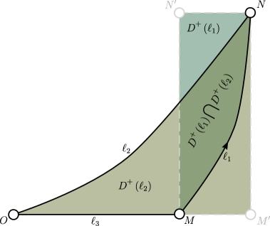
Figure 10.10: An illustration of the proof of theorem 10.6.2 for $n=3$ (the first case), where the domain’s edge is $\bigcup_{i=1}^{3}\ell_{i}$.

In case 1, as depicted in figure 10.10, we have that:

$$\begin{aligned} \underset{\ell_{1}}{\sqint}F&=\underset{D\left(\ell_{1}\right)}{\iint}f\boldsymbol{dx}-\ell_{1}^{;}F\left(N^{\prime}\right)+\frac{1}{2}\left[\gamma^{;}\left(M\right)F\left(M\right)+\gamma^{;}\left(N\right)F\left(N\right)\right],\\ \underset{\ell_{2}}{\sqint}F&=\underset{D\left(\ell_{2}\right)}{\iint}f\boldsymbol{dx}-\ell_{1}^{;}F\left(M^{\prime}\right)+\frac{1}{2}\left[\gamma^{;}\left(N\right)F\left(N\right)+\gamma^{;}\left(O\right)F\left(O\right)\right],\\ \underset{\ell_{3}}{\sqint}F&=\frac{1}{2}\left[\gamma^{;}\left(O\right)F\left(O\right)+\gamma^{;}\left(M\right)F\left(M\right)\right].\end{aligned}$$ (10.10)

Hence, in the illustrated case, it holds that:

$$\begin{aligned} \underset{\partial D}{\sqint}F&=\underset{\ell_{1}}{\sqint}F+\underset{\ell_{2}}{\sqint}F+\underset{\ell_{3}}{\sqint}F\\ &=\underset{D\left(\ell_{1}\right)\bigcup D\left(\ell_{2}\right)}{\iint}f\boldsymbol{dx}-\left[F\left(N\right)-F\left(N^{\prime}\right)+F\left(M\right)-F\left(M^{\prime}\right)\right]\\ &=\underset{D}{\iint}f\boldsymbol{dx},\end{aligned}$$ (10.11)

where the last transition is, once again, due to theorem 10.1.1.

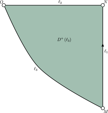
Figure 10.11: An illustration of the proof of theorem 10.6.2 for $n=3$ (the second case), where the domain’s edge is $\bigcup_{i=1}^{3}\ell_{i}$.

In case 2, as depicted in Figure 10.11, we have that:

$$\begin{aligned} \underset{\ell_{1}}{\sqint}F&=\frac{1}{2}\left[\gamma^{;}\left(M\right)F\left(M\right)+\gamma^{;}\left(N\right)F\left(N\right)\right],\\ \underset{\ell_{2}}{\sqint}F&=\frac{1}{2}\left[\gamma^{;}\left(N\right)F\left(N\right)+\gamma^{;}\left(O\right)F\left(O\right)\right],\\ \underset{\ell_{3}}{\sqint}F&=\underset{D\left(\ell_{3}\right)}{\iint}f\boldsymbol{dx}-\ell_{3}^{;}F\left(N\right)+\frac{1}{2}\left[\gamma^{;}\left(O\right)F\left(O\right)+\gamma^{;}\left(M\right)F\left(M\right)\right].\end{aligned}$$ (10.12)

Hence, in the illustrated case, it holds that:

$$\underset{\partial D}{\sqint}F=\underset{\ell_{1}}{\sqint}F+\underset{\ell_{2}}{\sqint}F+\underset{\ell_{3}}{\sqint}F=\underset{D\left(\ell_{3}\right)}{\iint}f\boldsymbol{dx}+f\left(N\right)-F\left(N\right)=\underset{D}{\iint}f\boldsymbol{dx}.$$

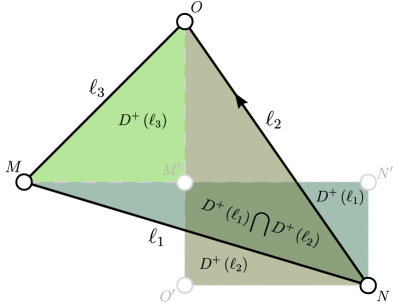
Figure 10.12: An illustration of the proof of theorem 10.6.2 for $n=3$ (the third case), where the domain’s edge is $\bigcup_{i=1}^{3}\ell_{i}$.

In case 3, as depicted in figure 10.12, we have:

$$\begin{aligned} \underset{\ell_{1}}{\sqint}F&=\underset{D\left(\ell_{1}\right)}{\iint}f\boldsymbol{dx}-\ell_{1}^{;}F\left(N^{\prime}\right)+\frac{1}{2}\left[\gamma^{;}\left(M\right)F\left(M\right)+\gamma^{;}\left(N\right)F\left(N\right)\right],\\ \underset{\ell_{2}}{\sqint}F&=\underset{D\left(\ell_{2}\right)}{\iint}f\boldsymbol{dx}-\ell_{2}^{;}F\left(O^{\prime}\right)+\frac{1}{2}\left[\gamma^{;}\left(N\right)F\left(N\right)+\gamma^{;}\left(O\right)F\left(O\right)\right],\\ \underset{\ell_{3}}{\sqint}F&=\underset{D\left(\ell_{3}\right)}{\iint}f\boldsymbol{dx}-\ell_{3}^{;}F\left(M^{\prime}\right)+\frac{1}{2}\left[\gamma^{;}\left(O\right)F\left(O\right)+\gamma^{;}\left(M\right)F\left(M\right)\right].\end{aligned}$$ (10.13)

Hence, in the illustrated case it holds that:

$$\underset{\partial D}{\sqint}F=\underset{\ell_{1}}{\sqint}F+\underset{\ell_{2}}{\sqint}F+\underset{\ell_{3}}{\sqint}F=\underset{D\left(\ell_{1}\right)\bigcup D\left(\ell_{2}\right)}{\iint}f\boldsymbol{dx}-\underset{D\left(\ell_{3}\right)}{\iint}f\boldsymbol{dx}=\underset{D}{\iint}f\boldsymbol{dx}.$$

Let us now apply the induction’s step. Suppose that the theorem holds for any domain whose boundary consists of less than $n$ monotonic subcurves. Let $D$ be a domain whose boundary, $\partial D$, is written as a minimal monotonic division of $n+1$ monotonic subcurves. Let us divide $D$ into two subdomains, $D_{\alpha}$ and $D_{\beta}$ , by connecting (via a straight line) between the disjoint endpoints of two adjacent monotonic subcurves of the division (such as the line $\overrightarrow{OM}$ in figure 10.8). According to lemma 10.6.1, it holds that:

$$\underset{\partial D}{\sqint}F=\underset{\partial D_{\alpha}}{\sqint}F+\underset{\partial D_{\beta}}{\sqint}F,$$

however, according to the induction hypothesis, and since $\partial D_{\alpha}$ and $\partial D_{\beta}$ both consist of at most $n$ monotonic subcurves, it holds that:

$$\underset{\partial D_{\alpha}}{\sqint}F=\underset{D_{\alpha}}{\iint}f\boldsymbol{dx},\quad\underset{\partial D_{\beta}}{\sqint}F=\underset{D_{\beta}}{\iint}f\boldsymbol{dx}.$$

Furthermore, according to the definition, $D_{\alpha}\bigcup D_{\beta}=D$, hence:

$$\underset{\partial D}{\sqint}F=\underset{\partial D_{\alpha}}{\sqint}F+\underset{\partial D_{\beta}}{\sqint}F=\underset{D\left(\ell_{1}\right)\bigcup D\left(\ell_{2}\right)}{\iint}f\boldsymbol{dx}=\underset{D}{\iint}f\boldsymbol{dx}.$$

∎

Note that the formulation of theorem 10.6.2 is a semi-discrete analog of Green’s theorem; it relates the double integral of a function in a domain with the semi-discrete line integral of the antiderivative along the domain’s edge. This is a concise version of corollary 10.1.2. One may opt to apply either version, according to the use case and requirements. The formulation of the former is concise due to the encapsulation embodied in the semi-discrete line integral. The later, however, is slightly more verbose; however, it may be more convenient in cases where one prefers to refrain from applying this new integration method.

Example 10.6.2 

Let us apply the semi-discrete line integral to a domain formed by a finite unification of rectangles, and see in which sense theorem 10.6.2 consolidates with theorem 10.1.1 for such domains. Let $f:\mathbb{R}^{2}\rightarrow\mathbb{R}$ be a function that admits an antiderivative $F$.

For a rectangle $ABCD$ whose edges are parallel to the axes, it holds that:

$$\begin{aligned} \underset{BADC}{\sqint}F&=\underset{\overrightarrow{BA}}{\sqint}F+\underset{\overrightarrow{AD}}{\sqint}F+\underset{\overrightarrow{DC}}{\sqint}F+\underset{\overrightarrow{CB}}{\sqint}F\\ &=\frac{1}{2}\left[+F\left(B\right)-F\left(A\right)\right]+\frac{1}{2}\left[+F\left(D\right)-F\left(A\right)\right]\\ &\quad+\frac{1}{2}\left[+F\left(D\right)-F\left(C\right)\right]+\frac{1}{2}\left[+F\left(B\right)-F\left(C\right)\right]\\ &=F\left(B\right)+F\left(D\right)-\left[F\left(A\right)+F\left(C\right)\right].\end{aligned}$$ (10.14)

More generally, applying the semi-discrete line integral to the edge of a rectangular domain results in a linear combination of the antiderivative at the corners, where each coefficient (that equals the value of $\alpha_{D}$ ) is determined according to the detachments (each half is provided by the discrete line integral over curves from either side of the corner). This case is depicted in figure 10.13.

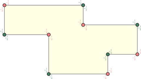
Figure 10.13: An illustration of theorem 10.6.2 for a finite unification of rectangles

Example 10.6.3 

Finally, let us verify the theorem’s correctness for non-convex domains. Let us apply the semi-discrete line integral to a detachable curve $\gamma$ (where $\gamma=\partial D$), as depicted in figure 10.14. Let $f:\mathbb{R}^{2}\rightarrow\mathbb{R}$ be a function that admits an antiderivative $F$.

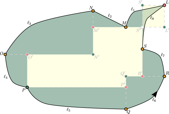
Figure 10.14: An illustration of theorem 10.6.2 with a domain that is partly convex and partly convex, where the domain’s edge is $\bigcup_{i=1}^{8}\ell_{i}$.

It holds that:

$$\begin{aligned} \underset{\gamma_{1}}{\sqint}F&=\underset{D\left(\gamma_{1}\right)}{\iint}f\boldsymbol{dx}-\frac{1}{2}F\left(L\right)+F\left(L^{\prime}\right),\\ \underset{\gamma_{2}}{\sqint}F&=\underset{D\left(\gamma_{2}\right)}{\iint}f\boldsymbol{dx}-F\left(M^{\prime}\right),\\ \underset{\gamma_{3}}{\sqint}F&=\underset{D\left(\gamma_{3}\right)}{\iint}f\boldsymbol{dx}+F\left(N^{\prime}\right),\\ \underset{\gamma_{4}}{\sqint}F&=\underset{D\left(\gamma_{4}\right)}{\iint}f\boldsymbol{dx}+\frac{1}{2}F\left(P\right)-F\left(O^{\prime}\right),\\ \underset{\gamma_{5}}{\sqint}F&=\underset{D\left(\gamma_{5}\right)}{\iint}f\boldsymbol{dx}+\frac{1}{2}F\left(P\right)-F\left(P^{\prime}\right),\\ \underset{\gamma_{6}}{\sqint}F&=\underset{D\left(\gamma_{6}\right)}{\iint}f\boldsymbol{dx}+F\left(Q^{\prime}\right),\\ \underset{\gamma_{7}}{\sqint}F&=\underset{D\left(\gamma_{7}\right)}{\iint}f\boldsymbol{dx}-F\left(R^{\prime}\right),\\ \underset{\gamma_{8}}{\sqint}F&=\underset{D\left(\gamma_{8}\right)}{\iint}f\boldsymbol{dx}-\frac{1}{2}F\left(L\right)+F\left(S^{\prime}\right).\end{aligned}$$ (10.15)

Adding up these equations, while considering the equality

$$\underset{L^{\prime}S^{\prime}S^{\prime\prime}L}{\iint}f\boldsymbol{dx}=F\left(S\right)-F\left(S^{\prime}\right)+F\left(S^{\prime\prime}\right)-F\left(L^{\prime}\right)$$

and applying theorem 10.1.1, results with $\underset{\gamma}{\sqint}F=\underset{D}{\iint}f\boldsymbol{dx}$ as theorem 10.6.2 states. Note that in the concave portion of the domain, the theorem subtracts the function’s integral over the rectangular domain $LS^{\prime}S^{\prime\prime}L^{\prime}$. This is the reason that the detachments of the curve at the point $L$ and along the curves $\ell_{1},\ell_{8}$ are flipped by construction.

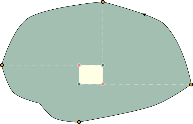
(a)

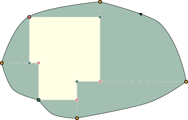
(b)

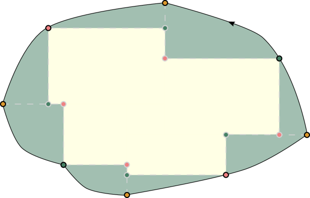
(c)

Figure 10.15: An illustration of different monotonic divisions of the same closed curve (the upper is the minimal such division) when applied in theorem 10.6.2. The subtler the division is, the larger the internal rectangular domain becomes - over whom the integral is calculated by aggregating the antiderivative’s values at the endpoints of each monotonic curve’s (positive) local domain.

Chapter 11 Semi-discrete Complex Analysis

Can we apply the detachment operator in the Complex plane? As in Real Analysis, a theory based on the derivative sign would go through rates calculations and be trivial. But what if we can introduce a theory about the properties of “complex trends” while calculating them directly without going through the derivative? Would this theory apply to non-differentiable and even discontinuous functions, similar to the case in Real Analysis? And would it capture trends in the function’s image more reliably and coherently than the derivative sign?

Complex Analysis is abundant with concepts that generalize their Real Analysis counterparts, such as continuity and the derivative. Inspired by its AI, natural sciences, and Real Analysis applications, let us consider a complex version of a function’s detachment and analyze its basic mathematical properties.

11.1 Defining the Complex Detachment

Recall that the signum of a complex number $z$ is defined as:

$$\text{sgn}\left(z\right)\equiv\frac{z}{\left|z\right|}=e^{iarg\left(z\right)},$$

where $arg\left(\cdot\right)$ is the complex argument function. Geometrically, this means that the sign function maps any point in the complex plane to its closest counterpart on the unit circle, as illustrated in Figure 11.1.

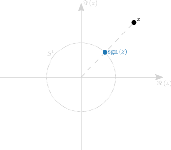
Figure 11.1: An illustration of the complex signum function

Note that in Real Analysis, we suggested softening the definition of the detachment with respect to the derivative by considering merely one-sided detachments, defined by one-sided limits, and did not require them to agree. We naturally extend the notion of one-sided derivatives in higher dimensions with directional derivatives. The Complex Analysis literature conventionally focuses on differentiable and, more specifically, analytic functions. However, complex partial derivatives, also known as Wirtinger derivatives, are prevalent. They particularly serve to define the complex directional derivatives, which are useful as well, depending on the context. For example, they are applied in advanced research (see [299]), and also serve as a pedagogical and auxiliary thought tool (see [875]). Let us suggest an analogous natural way to define the directional detachment.

Definition 11.1.1 — Detachment of a complex function. 

Let us define the $\varphi$-detachment of a function $f:\mathbb{C}\longrightarrow\mathbb{C}$ at a point $z_{0}\in\mathbb{C}$ as follows:

$$\begin{array}[]{ccc}&f_{\varphi}^{;}:\mathbb{C}\longrightarrow S^{1}\bigcup\left\{0\right\}\\ &f_{\varphi}^{;}\left(z_{0}\right)\equiv e^{-i\varphi}\underset{\begin{array}[]{c}\left|z\right|\to\left|z_{0}\right|\\ \arg\left(\Delta z\right)=\varphi\end{array}}{\lim}\text{sgn}\left[f\left(z\right)-f\left(z_{0}\right)\right],\end{array}$$

where $S^{1}$ is the unit circle in the complex plane. We will say that $f$ is $\varphi$-detachable at $z_{0}$ if the limit exists.

We may think of the $e^{-i\varphi}$ coefficient as a generalization of the $\pm 1$ coefficient from the one-sided detachment in Real Analysis. Both coefficients render the detachment more consistent with the derivative sign, as shown in the following statement.

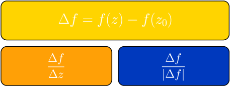
Figure 11.2: In the complex detachment we divide $\Delta f$ by its norm (as in the definition of the signum function), rather than by $\Delta z$ as in the complex derivative.

The following claim shows that the detachment adds a calculation value with respect to the derivative only in cases where the derivative vanishes.

Claim 11.1.1 

If $f:\mathbb{C}\longrightarrow\mathbb{C}$ is both differentiable and $\varphi$-detachable at the point $z_{0},$ and $f^{\prime}\left(z_{0}\right)\neq 0,$ then:

$$f_{\varphi}^{;}\left(z_{0}\right)=\text{sgn}\left[\frac{\partial f}{\partial\varphi}\left(z_{0}\right)\right].$$

Proof.

According to the definition:

$$\begin{aligned} f_{\varphi}^{;}\left(z_{0}\right)&\equiv e^{-i\varphi}\underset{\begin{array}[]{c}\left|z\right|\to\left|z_{0}\right|\\ \arg\left(\Delta z\right)=\varphi\end{array}}{\lim}\text{sgn}\left[f\left(z\right)-f\left(z_{0}\right)\right]=\underset{\begin{array}[]{c}\left|z\right|\to\left|z_{0}\right|\\ \arg\left(\Delta z\right)=\varphi\end{array}}{\lim}\frac{\text{sgn}\left[f\left(z\right)-f\left(z_{0}\right)\right]}{e^{i\varphi}}\\ &=\underset{\begin{array}[]{c}\left|z\right|\to\left|z_{0}\right|\\ \arg\left(\Delta z\right)=\varphi\end{array}}{\lim}\frac{\text{sgn}\left[f\left(z\right)-f\left(z_{0}\right)\right]}{\text{sgn}\left(z-z_{0}\right)}=\underset{\begin{array}[]{c}\left|z\right|\to\left|z_{0}\right|\\ \arg\left(\Delta z\right)=\varphi\end{array}}{\lim}\text{sgn}\left[\frac{f\left(z\right)-f\left(z_{0}\right)}{z-z_{0}}\right]\\ &=\text{sgn}\underset{\begin{array}[]{c}\left|z\right|\to\left|z_{0}\right|\\ \arg\left(\Delta z\right)=\varphi\end{array}}{\lim}\left[\frac{f\left(z\right)-f\left(z_{0}\right)}{z-z_{0}}\right]=\text{sgn}\left[\frac{\partial f}{\partial\varphi}\left(z_{0}\right)\right],\end{aligned}$$ (11.1)

where the fifth transition is because the sign function is continuous in $\mathbb{C}\backslash\left\{0\right\}$. ∎

For brevity, we will denote the $\varphi$-detachment at the point $z_{0}$ by $f^{;},$ rather than $f_{\varphi}^{;}\left(z_{0}\right)$.

11.2 Geometric Intuition

Suppose that a function is $\varphi$-detachable at $z_{0}.$ Then, by the limit definition, given $\epsilon>0,$ for any sufficiently small environment of $z_{0},$ the function’s values at a point $z$, satisfy that:

$$\left|\text{sgn}\left[f\left(z\right)-f\left(z_{0}\right)\right]-f^{;}\right|<\epsilon.$$

This means that $f\left(z\right)$ is bounded between two lines intersecting at $z_{0}.$ The angle between the spanning vector of each line and $f^{;},$ is $\epsilon.$

Recall that, in the realm of the real functions, the detachment definition is equivalent to the following statement:

$$\exists\dot{B}_{\pm}\left(x_{0}\right):\forall x\in\dot{B}_{\pm}\left(x_{0}\right):\,\,\,\,\,\text{sgn}\left[f\left(x\right)-f\left(x_{0}\right)\right]=f_{\pm}^{;}\left(x_{0}\right),$$

due to the discontinuity of the sign function at zero.

However, an analogous statement in the complex domain does not necessarily hold. Such a statement is more strict than the existence of the limit stated in equation 11.1.1. Geometrically, the former is defined merely for functions whose image near a point is on a straight line. The reason lies in the different geometric interpretations of the discontinuity of the sign function in one vs. two dimensional functions.

We know that the limit $\underset{z\to 0}{\lim}\text{sgn}\left(z\right)$ does not exists because it depends on the different paths by which we let $z$ approach zero. Can this intuition help us establish a geometric interpretation for the detachment?

The detachability of a real valued function at a point is a synonymous with the function having a “local trend”. The detachability of a complex function points out the existence of a “local trend” in a broader sense.

Intuitively, a $\theta$-detachable function maps points along a line in the environment of the point, to points “approaching” a single line.

The differentiability of a function at a point allows us to calculate its values with the linear approximation formula; it states that the function’s value is linear in the difference between the points (up to the function $\rho$):

$$f\left(z\right)=f\left(z_{0}\right)+f^{\prime}\left(z_{0}\right)\left(z-z_{0}\right)+\rho\left(z\right)\left(z-z_{0}\right),$$

where $\underset{z\to z_{0}}{\lim}\rho\left(z\right)=0$ and $z\neq z_{0}.$

In contrast, the detachment suggests a different kind of approximated linear relation of the function’s image, where the formula itself does not involve information from the domain. Suppose $f$ is $\varphi$-detachable, and let $\epsilon>0.$ According to the limit definition, we have that for $z$ in a sufficiently small environment of $z_{0}$ such that $\arg\left(z-z_{0}\right)=\varphi$:

$$\left|\text{sgn}\left[f\left(z\right)-f\left(z_{0}\right)\right]-f^{;}e^{i\varphi}\right|<\epsilon.$$

Since $f^{;}$ is the limit of points on the (closed) unit circle, it has to be on the circle as well. The size of the chord between $\text{sgn}\left[f\left(z\right)-f\left(z_{0}\right)\right]$ and $f^{;}e^{i\varphi}$ is at most $\epsilon.$ Let us assume, without loss of generality, that $0<\arg\left(f^{;}e^{i\varphi}\right)<\frac{\pi}{2}.$

Let $\theta_{f}$ be the angle between $\text{sgn}\left[f\left(z\right)-f\left(z_{0}\right)\right]$ and $f^{;}e^{i\varphi}.$ The formula for the size of a chord given the angle $\theta_{f}$ and radius $1$ yields:

$$\left|\text{sgn}\left[f\left(z\right)-f\left(z_{0}\right)\right]-f^{;}e^{i\varphi}\right|=2\cdot 1\cdot\sin\left(\frac{\theta_{f}}{2}\right),$$

hence:

$$\theta_{f}=2\arcsin\left(\frac{\left|\text{sgn}\left[f\left(z\right)-f\left(z_{0}\right)\right]-f^{;}e^{i\varphi}\right|}{2}\right)<2\arcsin\left(\frac{\epsilon}{2}\right).$$

Therefore, we show that the argument of the difference between the function’s image at points in the environment of $z_{0}$ and its image at $z_{0}$ satisfies:

$$arg\left(f\left(z\right)-f\left(z_{0}\right)\right)\in\left(\arg\left(f^{;}e^{i\varphi}\right)-2\arcsin\left(\frac{\epsilon}{2}\right),\arg\left(f^{;}e^{i\varphi}\right)+2\arcsin\left(\frac{\epsilon}{2}\right)\right).$$

We will refer to the above analysis, which associates the bound and the chord length with these of the angle, as a “chord-angle” analysis.

11.3 Computability and Consistency

Similar to the case in Real Analysis, detachability at a point does not necessarily implies continuity or differentiability - and vice versa. Let us illustrate some basic examples to gain a better understanding of why this is the case.

Example 11.3.1 

Let us consider the following function:

$$f\left(z\right)=\begin{cases}\frac{1}{z},&z\neq 0,\\ 0,&z=0.\end{cases}$$

Let us calculate the $\varphi$-detachments by the definition:

$$f_{\varphi}^{;}\left(0\right)\equiv e^{-i\varphi}\underset{\begin{array}[]{c}\left|z\right|\to\left|z_{0}\right|\\ \arg\left(\Delta z\right)=\varphi\end{array}}{\lim}\text{sgn}\left[f\left(z\right)-f\left(z_{0}\right)\right]=e^{-i\varphi}\cdot\underset{\begin{array}[]{c}\left|z\right|\to\left|z_{0}\right|\\ \arg\left(\Delta z\right)=\varphi\end{array}}{\lim}\left[\frac{1}{\text{sgn}\left(z\right)}\right]=e^{-2i\varphi}.$$

This is an example of a non-differentiable and discontinuous function, for which the detachment is nevertheless able to provide monotony information.

Example 11.3.2 

Let $f\left(z\right)=z^{2}.$ The derivative is $f^{\prime}\left(z_{0}\right)=2z_{0}.$ Particularly, at $z_{0}=0$ the derivative vanishes and we ought to calculate the detachment based on its definition:

$$f_{\varphi}^{;}\left(0\right)\equiv e^{-i\varphi}\underset{\begin{array}[]{c}\left|z\right|\to\left|z_{0}\right|\\ \arg\left(\Delta z\right)=\varphi\end{array}}{\lim}\text{sgn}\left[f\left(z\right)-f\left(z_{0}\right)\right]=e^{-i\varphi}\underset{\begin{array}[]{c}\left|z\right|\to\left|z_{0}\right|\\ \arg\left(\Delta z\right)=\varphi\end{array}}{\lim}\text{sgn}\left(z^{2}\right)=e^{-i\varphi}\cdot e^{2i\varphi}=e^{i\varphi}.$$

Thus, similarly to the case in Real Analysis, while the directional derivatives do not provide monotony information at the stationary point, the directional detachment does.

Example 11.3.3 

Let $f\left(z\right)=\sqrt{z}.$ The derivative is $f^{\prime}\left(z_{0}\right)=\frac{1}{2\sqrt{z_{0}}}.$ At $z_{0}=0$, the derivative does not exist and we ought to calculate the detachment based on its definition:

$$f_{\varphi}^{;}\left(0\right)\equiv\underset{\begin{array}[]{c}\left|z\right|\to\left|z_{0}\right|\\ \arg\left(\Delta z\right)=\varphi_{2}\end{array}}{\lim}\text{sgn}\left[f\left(z\right)-f\left(z_{0}\right)\right]=\underset{\begin{array}[]{c}\left|z\right|\to\left|z_{0}\right|\\ \arg\left(z\right)=\varphi_{2}\end{array}}{\lim}\text{sgn}\left(\sqrt{z}\right)=e^{\frac{i\varphi}{2}}.$$

As such, similarly to the case in Real Analysis, the detachment may also provide monotony information at the derivative’s singularities for continuous functions.

Example 11.3.4 

Let

$$f\left(z\right)=\begin{cases}z\sin\left(z\right),&z\neq 0,\\ 0,&z=0.\end{cases}$$

Then $f$ is differentiable at $z=0,$ but the definition of its directional detachment yields:

$$\begin{aligned} f_{\varphi}^{;}\left(0\right)&\equiv\underset{\begin{array}[]{c}\left|z\right|\to\left|z_{0}\right|\\ \arg\left(\Delta z\right)=\varphi_{2}\end{array}}{\lim}\text{sgn}\left[f\left(z\right)-f\left(z_{0}\right)\right]=\underset{\begin{array}[]{c}\left|z\right|\to\left|z_{0}\right|\\ \arg\left(z\right)=\varphi_{2}\end{array}}{\lim}\text{sgn}\left(z\sin\left(z\right)\right)\\ &=e^{i\varphi}\underset{\begin{array}[]{c}\left|z\right|\to\left|z_{0}\right|\\ \arg\left(\Delta z\right)=\varphi_{2}\end{array}}{\lim}\text{sgn}\left[\sin\left(z\right)\right],\end{aligned}$$ (11.2)

which is undefined. Thus, similarly to the case in Real Analysis, the complex detachment may not provide monotony information at points of infinite oscillations.

Example 11.3.5 

Let $f\left(z\right)=\Re\left(z\right),$ whose image is the real line. The sign of its directional derivative satisfies:

$$\text{sgn}\left[\frac{\partial f}{\partial\varphi}\left(z_{0}\right)\right]\equiv\text{sgn}\left\{\underset{\begin{array}[]{c}\left|z\right|\to\left|z_{0}\right|\\ \arg\left(\Delta z\right)=\varphi\end{array}}{\lim}\left[\frac{\Re\left(\Delta z\right)}{\Delta z}\right]\right\}=\text{sgn}\left[\cos\left(\varphi\right)e^{-i\varphi}\right]=\begin{cases}e^{-i\varphi},&\left|\varphi\right|<\frac{\pi}{2},\\ 0,&\left|\varphi\right|=\frac{\pi}{2},\\ -e^{-i\varphi},&\text{else},\end{cases}.$$

Since the derivative may vanish, let us calculate the $\varphi$-detachment directly according to the definition:

$$\begin{aligned} f_{\varphi}^{;}\left(z_{0}\right)&\equiv e^{-i\varphi}\underset{\begin{array}[]{c}\left|z\right|\to\left|z_{0}\right|\\ \arg\left(\Delta z\right)=\varphi\end{array}}{\lim}\text{sgn}\left[f\left(z\right)-f\left(z_{0}\right)\right]\\ &=e^{-i\varphi}\underset{\begin{array}[]{c}\left|z\right|\to\left|z_{0}\right|\\ \arg\left(\Delta z\right)=\varphi\end{array}}{\lim}\text{sgn}\left[\Re\left(\Delta z\right)\right]=\begin{cases}e^{-i\varphi},&\left|\varphi\right|<\frac{\pi}{2},\\ 0,&\left|\varphi\right|=\frac{\pi}{2},\\ -e^{-i\varphi},&\text{else}.\end{cases}\end{aligned}$$ (11.3)

This is an example where the detachment agrees with the derivative sign even in cases where it vanishes ($\left|\varphi\right|=\frac{\pi}{2}$ in this example).

11.4 Auxiliary Terminology

Assumptions and abbreviations. We will apply the following notations below:

We focus on directional detachments in a given angle $\varphi.$ Therefore, by a $\delta$-“environment” of the point $z_{0}$, we refer to the $\delta$-lengthed line segment starting at $z_{0}$ and tilted by $\varphi$ with respect to $z_{0}.$ We assume, without loss of generality, that all the complex numbers’ arguments are between $0$ and $\pi.$ For the two variables $z_{0}$ and $z$ in the definition domain of a function $f,$ we apply the abbreviation $\Delta f=f\left(z\right)-f\left(z_{0}\right).$ The value of an operator applied to a function is calculated at $z_{0}$, unless we specifically mention otherwise; for example, $\text{sgn}\left(f\right)=\text{sgn}\left(f\left(z_{0}\right)\right).$

We assume detachability, but not differentiability nor continuity, of the functions involved in the results below. As a tradeoff, we will apply the following intuitive and useful concepts.

Definition 11.4.1 — Complex sign-continuity. 

Let $f:\mathbb{C}\longrightarrow\mathbb{C}$ be a function, and let $z_{0}\in\mathbb{C}.$ Then, $f$ is sign-continuous at $z_{0}$ if $\text{sgn}\left(f\right)$ is continuous.

Definition 11.4.2 — Bimodularity. 

Let $f,g:\mathbb{C}\longrightarrow\mathbb{C}$ be a pair of functions, and let $z_{0}\in\mathbb{C}.$ Then $f,g$ are:

• Bimodular at $z_{0}$ if for each $z$ in its neighborhood: $\left|\Delta f\right|=\left|\Delta g\right|.$

• Locally bimodular at $z_{0}$ if for each $z$ in its neighborhood, $\left|f\Delta g\right|=\left|g\Delta f\right|.$

• Spatially bimodular at $z_{0}$ if for each $z$ in its neighborhood, $\left|f\left(z\right)\Delta g\right|=\left|g\left(z\right)\Delta f\right|.$

Example 11.4.1 

Any complex function is sign-continuous whenever the function’s angle of change is continuous. This may happen at the point of non-differentiability, such as cusps. It may also happen at discontinuities, for example if the function’s graph approaches a line in a discontinuous fashion.

Example 11.4.2 

Any function $g:\mathbb{C}\longrightarrow\mathbb{C}$ is everywhere bimodular to all its reflections with respect to the axes:

$$g_{1}\left(z\right)=-f\left(z\right),g_{2}\left(z\right)=\overline{f\left(z\right)},g_{3}\left(z\right)=-\overline{f\left(z\right)},$$

and to all its rotations by a unit vector, $g_{4}\left(z\right)=f\left(z\right)e^{i\xi}.$

Example 11.4.3 

Let $f,g:\mathbb{C}\longrightarrow\mathbb{C},$ and let $z_{0}\in\mathbb{C}.$ If there is an environment where $g$ is a constant multiplication of $f,$ then they are locally and spatially bimodular. More precisely, if $g\neq 0$ and $\frac{f}{g}$ is continuous at $z_{0}$ and constant in its neighborhood, then $f,g$ are both locally and spatially bimodular at $z_{0}.$ Let us show local bimodularity. Given $z$ in an environment of $z_{0},$ where $\frac{f}{g}$ is held constant:

$$\left|f\left(z_{0}\right)\Delta g\right|=\left|\frac{f\left(z_{0}\right)}{g\left(z_{0}\right)}g\left(z_{0}\right)g\left(z\right)-f\left(z_{0}\right)g\left(z_{0}\right)\right|=\left|\frac{f\left(z\right)}{g\left(z\right)}g\left(z_{0}\right)g\left(z\right)-f\left(z_{0}\right)g\left(z_{0}\right)\right|=\left|g\left(z_{0}\right)\Delta f\right|,$$

where the fourth equality is due to the continuity and constancy of $\frac{f}{g}.$ A similar argument holds for their spatial bimodularity. Note that this condition is sufficient but not necessary for bimodularity.

Let $f:\mathbb{C}\longrightarrow\mathbb{C}$ be a detachable function and $z_{0}\in C.$ Let $\epsilon>0.$ We previously showed with a chord-angle analysis, that the detachability of a function $f$ implies that there is an environment of $z_{0}$ wherein:

$$\arg\left(\Delta f\right)\in\left(\arg\left(f^{;}e^{i\varphi}\right)-2\arcsin\left(\frac{\epsilon}{2}\right),\arg\left(f^{;}e^{i\varphi}\right)+2\arcsin\left(\frac{\epsilon}{2}\right)\right).$$

Let us use the following notation for brevity:

$$\theta_{f}\equiv\arg\left(\frac{\Delta f}{f^{;}e^{i\varphi}}\right)<2\arcsin\left(\frac{\epsilon}{2}\right),$$

where the equality can be rewritten as follows:

$$\text{sgn}\left(\Delta f\right)=f^{;}e^{i\left(\varphi+\theta_{f}\right)}.$$

Similarly, if $f$ is sign-continuous, then given $\epsilon>0,$ the limit definition ensures the existence of an environment such that for each $z$, $\left|\text{sgn}\left(f\left(z\right)\right)-\text{sgn}\left(f\right)\right|<\frac{\epsilon}{2},$ therefore $\text{sgn}\left(f\left(z\right)\right)\in\left(\text{sgn}\left(f\right)-\epsilon,\text{sgn}\left(f\right)+\epsilon\right).$ Let us use the following notation:

$$\theta\equiv\arg\left(f\left(z\right)\right)-\arg\left(f\left(z_{0}\right)\right),$$

which can be rewritten as

$$\text{sgn}\left(f\left(z\right)\right)=\text{sgn}\left(f\left(z_{0}\right)\right)e^{i\theta}.$$

Let us cite the following known result without proof.

Lemma 11.4.4 

Let $z_{1},z_{2}\in\mathbb{C}.$ If $\left|z_{1}\right|=\left|z_{2}\right|$ such that $0<\arg\left(z_{1}\right),\arg\left(z_{2}\right)<\pi$ then:

$$\arg\left(z_{1}+z_{2}\right)=\frac{\arg\left(z_{1}\right)+\arg\left(z_{2}\right)}{2}.$$

Lemma 11.4.5 

Let $f,g:\mathbb{C}\longrightarrow\mathbb{C}$ be detachable functions at $z_{0}\in\mathbb{C}$ and let $\epsilon>0.$ Then there is an environment of $z_{0}$ such that for each $z$ there:

$$\left|e^{\frac{i}{2}\left(\theta_{f}+\theta_{g}\right)}-1\right|<\epsilon.$$

Proof.

By the following transitions:

$$\left|e^{\frac{i}{2}\left(\theta_{f}+\theta_{g}\right)}-1\right|=2\sin\left(\frac{\theta_{f}+\theta_{g}}{4}\right)<2\sin\left(\frac{2\arcsin\left(\frac{\epsilon}{2}\right)+2\arcsin\left(\frac{\epsilon}{2}\right)}{4}\right)=\epsilon,$$

where the first equality is due to a chord-angle analysis of the angle $\frac{\theta_{f}+\theta_{g}}{2}$, the inequality is due to the upper bound provided in formula (11.4), applied to both $\theta_{f},\theta_{g}$, combined with the monotony of the $\sin$ function near zero. ∎

Lemma 11.4.6 

Let $f,g:\mathbb{C}\longrightarrow\mathbb{C}$ be detachable functions at $z_{0}\in\mathbb{C},$ where $f$ is sign-continuous. Let $\epsilon>0.$ Then there is an environment of $z_{0}$ such that for each $z$:

$$\left|e^{\frac{i}{2}\left(\theta+\theta_{f}+\theta_{g}\right)}-1\right|<\epsilon.$$

Proof.

From the sign continuity of $f$ we know that for each $z$ close enough to $z_{0}$:

$$\left|\text{sgn}\left(f\left(z\right)\right)-\text{sgn}\left(f\right)\right|<\frac{\epsilon}{2},$$

therefore $\text{sgn}\left(f\left(z\right)\right)\in\left(\text{sgn}\left(f\right)-\epsilon,\text{sgn}\left(f\right)+\epsilon\right),$ and a chord-angle analysis yields that we can bound the angle $\theta=\arg\left(f\left(z\right)\right)-\arg\left(f\left(z_{0}\right)\right),$ from above, by $2\arcsin\left(\frac{\epsilon}{4}\right).$

Thus, it holds that:

$$\begin{aligned} \left|e^{\frac{i}{2}\left(\theta+\theta_{f}+\theta_{g}\right)}-1\right|&=2\sin\left(\frac{\theta+\theta_{f}+\theta_{g}}{4}\right)<2\sin\left(\frac{2\arcsin\left(\frac{\epsilon}{4}\right)+2\arcsin\left(\frac{\epsilon}{4}\right)+2\arcsin\left(\frac{\epsilon}{4}\right)}{4}\right)\\ &=2\sin\left(\frac{3}{2}\arcsin\left(\frac{\epsilon}{4}\right)\right)<2\sin\left(2\arcsin\left(\frac{\epsilon}{4}\right)\right)\\ &=4\sin\left(\arcsin\left(\frac{\epsilon}{4}\right)\right)\cos\left(\arcsin\left(\frac{\epsilon}{4}\right)\right)\leq 4\sin\left(\arcsin\left(\frac{\epsilon}{4}\right)\right)=\epsilon\end{aligned}$$ (11.4)

∎

11.5 Algebraic Rules

Claim 11.5.1 

Constant multiple rule. Let $f:\mathbb{C}\longrightarrow\mathbb{C}$ be detachable at the point $z_{0}\in\mathbb{C}$, and let $c\in\mathbb{C}$. Then $cf$ is also detachable and:

$$\left(cf\right)^{;}=\text{sgn}\left(cf^{;}\right).$$

Proof.

Directly from the definition of the detachment:

$$\begin{aligned} \left(cf\right)^{;}\left(z_{0}\right)\equiv\underset{z\to z_{0}}{\lim}\text{sgn}\left[\left(cf\right)\left(z\right)-\left(cf\right)\left(z_{0}\right)\right]&=\underset{z\to z_{0}}{\lim}\text{sgn}\left[c\Delta f\right]\\ &=\underset{z\to z_{0}}{\lim}\text{sgn}\left(c\right)\text{sgn}\left(\Delta f\right)\\ &=\text{sgn}\left(c\right)\underset{z\to z_{0}}{\lim}\text{sgn}\left(\Delta f\right)\\ &=\text{sgn}\left(c\right)f^{;}=\text{sgn}\left(cf^{;}\right)\end{aligned}$$ (11.5)

∎

Theorem 11.5.1 — Sum rule. 

Let $f,g:\mathbb{C}\longrightarrow\mathbb{C}$ be detachable at $z_{0}\in\mathbb{C}$ and $f,g$ be bimodular at $z_{0}.$

Then $f\pm g$ is also detachable and:

$$\left(f\pm g\right)^{;}=\text{sgn}\left(f^{;}\pm g^{;}\right).$$

Proof.

Let $\epsilon>0.$ Without loss of generality, assume that $\arg\left(f^{;}\right)\leq\arg\left(g^{;}\right).$ Let us prove the formula for the sum, and leave the one for the difference as an exercise. There are $\delta$-environments of $z_{0}$, such that for each $z$ , the following conditions hold:

Environment	Condition	Reason
$\delta_{1}$	$\left|e^{\frac{i}{2}\left(\theta_{f}+\theta_{g}\right)}-1\right|<\epsilon$	Lemma 11.4.5, since $f$ and $g$ are detachable
$\delta_{2}$	$\left|\Delta f\right|=\left|\Delta g\right|$	$f,g$ are bimodular

Then, for each $z$ in the $\min\left\{\delta_{1},\delta_{2}\right\}$ -environment, it holds that:

$$\begin{aligned} &\left|\text{sgn}\left(\left(f+g\right)\left(z\right)-\left(f+g\right)\left(z_{0}\right)\right)-\text{sgn}\left(f^{;}+g^{;}\right)e^{i\varphi}\right|\\ &=\left|\text{sgn}\left(\Delta f+\Delta g\right)-\text{sgn}\left(f^{;}+g^{;}\right)e^{i\varphi}\right|\\ &=\left|\text{sgn}\left(\left|\Delta f\right|f^{;}e^{i\theta_{f}}e^{i\varphi}+\left|\Delta g\right|g^{;}e^{i\theta_{g}}e^{i\varphi}\right)-\text{sgn}\left(f^{;}+g^{;}\right)e^{i\varphi}\right|\\ &=\left|\text{sgn}\left(\left|\Delta f\right|f^{;}e^{i\theta_{f}}+\left|\Delta g\right|g^{;}e^{i\theta_{g}}\right)-\text{sgn}\left(f^{;}+g^{;}\right)\right|\\ &=\left|e^{i\arg\left[\left|\Delta f\right|f^{;}e^{i\theta_{f}}+\left|\Delta g\right|g^{;}e^{i\theta_{g}}\right]}-e^{\frac{i}{2}\left[\arg\left(f^{;}\right)+\arg\left(g^{;}\right)\right]}\right|\\ &=\left|e^{\frac{i}{2}\left[\arg\left(f^{;}e^{i\theta_{f}}\right)+\arg\left(g^{;}e^{i\theta_{g}}\right)\right]}-e^{\frac{i}{2}\left[\arg\left(f^{;}\right)+\arg\left(g^{;}\right)\right]}\right|\\ &=\left|e^{\frac{i}{2}\left[\arg\left(f^{;}\right)+\theta_{f}+\arg\left(g^{;}\right)+\theta_{g}\right]}-e^{\frac{i}{2}\left[\arg\left(f^{;}\right)+\arg\left(g^{;}\right)\right]}\right|\\ &=\left|e^{\frac{i}{2}\left[\arg\left(f^{;}\right)+\arg\left(g^{;}\right)\right]}\left\{e^{\frac{i}{2}\left(\theta_{f}+\theta_{g}\right)}-1\right\}\right|\\ &=\left|e^{\frac{i}{2}\left(\theta_{f}+\theta_{g}\right)}-1\right|<\epsilon,\end{aligned}$$ (11.6)

where the second transition is due to the notation in formula 11.4, the fifth transition is due to the third condition above and formula (11.4.4). The inequality is due to the first condition. ∎

Theorem 11.5.2 — Product rule. 

Let $f,g:\mathbb{C}\longrightarrow\mathbb{C}$ be spatially bimodular and detachable at the point $z_{0}\in\mathbb{C}.$ Assume that $f$ is sign-continuous, and $g,g(z_{0})$ are bimodular, or vice versa, at $z_{0}.$ Then, $fg$ is also detachable at $z_{0},$ and:

$$\left(fg\right)^{;}=\text{sgn}\left[f^{;}\text{sgn}\left(g\right)+g^{;}\text{sgn}\left(f\right)\right].$$

Proof.

Let $\epsilon>0,$ and, without loss of generality, assume that $f$ is sign continuous and $g,g\left(z_{0}\right)$ are bimodular at $z_{0}.$ There are $\delta$-environments, such that for each $z$, the following conditions hold:

Environment	Condition	Reason
$\delta_{1}$	$\left|e^{\frac{i}{2}\left(\theta+\theta_{f}+\theta_{g}\right)}-1\right|<\epsilon$	Lemma 11.4.6, since $f$ and $g$ are detachable
$\delta_{2}$	$\left|g\left(z\right)\right|=\left|g\right|$	$g,g\left(z_{0}\right)$ are bimodular
$\delta_{3}$	$\left|f(z)\Delta g\right|=\left|g(z)\Delta f\right|$	$f,g$ are spatially bimodular

Let $z$ in the $\min\left\{\delta_{1},\delta_{2},\delta_{3}\right\}$-environment. Then:

$$\begin{aligned} &\left|\text{sgn}\left[\left(fg\right)\left(z\right)-\left(fg\right)\left(z_{0}\right)\right]-\text{sgn}\left[f^{;}\text{sgn}\left(g\right)+g^{;}\text{sgn}\left(f\right)\right]e^{i\varphi}\right|\\ &=\left|\text{sgn}\left[f\left(z\right)g\left(z\right)-f\left(z\right)g\left(z_{0}\right)+f\left(z\right)g\left(z_{0}\right)-f\left(z\right)g\left(z_{0}\right)\right]-\text{sgn}\left[f^{;}\text{sgn}\left(g\right)+g^{;}\text{sgn}\left(f\right)\right]e^{i\varphi}\right|\\ &=\left|\text{sgn}\left[f\left(z\right)\Delta g+g\left(z_{0}\right)\Delta f\right]-\text{sgn}\left[f^{;}\text{sgn}\left(g\right)+g^{;}\text{sgn}\left(f\right)\right]e^{i\varphi}\right|\\ &=\left|\text{sgn}\left[\left|f\left(z\right)\right|\text{sgn}\left(f\left(z\right)\right)\left|\Delta g\right|\text{sgn}\left(\Delta g\right)+\left|g\left(z_{0}\right)\right|\text{sgn}\left(g\right)\left|\Delta f\right|\text{sgn}\left(\Delta f\right)\right]-\text{sgn}\left[f^{;}\text{sgn}\left(g\right)+g^{;}\text{sgn}\left(f\right)\right]e^{i\varphi}\right|\\ &=\left|\text{sgn}\left[\left|f\left(z\right)\right|\text{sgn}\left(f\right)e^{i\theta}\left|\Delta g\right|g^{;}e^{i\theta_{g}}e^{i\varphi}+\left|g\left(z\right)\right|\text{sgn}\left(g\right)\left|\Delta f\right|f^{;}e^{i\theta_{f}}e^{i\varphi}\right]-\text{sgn}\left[f^{;}\text{sgn}\left(g\right)+g^{;}\text{sgn}\left(f\right)\right]e^{i\varphi}\right|\\ &=\left|\text{sgn}\left[\text{sgn}\left(f\right)e^{i\theta}g^{;}e^{i\theta_{g}}+\text{sgn}\left(g\right)f^{;}e^{i\theta_{f}}\right]-\text{sgn}\left[f^{;}\text{sgn}\left(g\right)+g^{;}\text{sgn}\left(f\right)\right]\right|\\ &=\left|e^{i\left[\text{sgn}\left(f\right)e^{i\theta}g^{;}e^{i\theta_{g}}+\text{sgn}\left(g\right)f^{;}e^{i\theta_{f}}\right]}-e^{i\left[f^{;}\text{sgn}\left(g\right)+g^{;}\text{sgn}\left(f\right)\right]}\right|\\ &=\left|e^{\frac{i}{2}\left[\arg\left(f\right)+\theta+\arg\left(g^{;}\right)+\theta_{g}+\arg\left(g\right)+\arg\left(f^{;}\right)+\theta_{f}\right]}-e^{\frac{i}{2}\left[\arg\left(f\right)+\arg\left(g^{;}\right)+\arg\left(g\right)+\arg\left(f^{;}\right)\right]}\right|\\ &=\left|e^{\frac{i}{2}\left[\arg\left(f\right)+\arg\left(g^{;}\right)+\arg\left(g\right)+\arg\left(f^{;}\right)\right]}\left[e^{\frac{i}{2}\left(\theta+\theta_{f}+\theta_{g}\right)}-1\right]\right|=\left|e^{\frac{i}{2}\left(\theta+\theta_{f}+\theta_{g}\right)}-1\right|<\epsilon,\end{aligned}$$ (11.7)

where the fourth transition is due to the notation in formula 11.4 and due to the second and third conditions above, the seventh transition is due to lemma 11.4.4, and the inequality is due to lemma 11.4.6. ∎

Theorem 11.5.3 

Quotient rule. Let $f,g\neq 0:\mathbb{C}\longrightarrow\mathbb{C}$ be locally bimodular and detachable at the point $z_{0}\in\mathbb{C},$ where $g$ is sign-continuous at $z_{0}.$ Then $\frac{f}{g}$ is also detachable, and:

$$\left(\frac{f}{g}\right)^{;}=\text{sgn}\left[\frac{\text{sgn}\left(g\right)f^{;}-\text{sgn}\left(f\right)g^{;}}{g^{2}}\right].$$

Proof.

First, let us develop the expression by the definition of the limit:

$$\begin{aligned} \left(\frac{f}{g}\right)^{;}&\equiv e^{-i\varphi}\underset{z\to z_{0}}{\lim}\text{sgn}\left[\left(\frac{f}{g}\right)\left(z\right)-\left(\frac{f}{g}\right)\left(z_{0}\right)\right]\\ &=\underset{z\to z_{0}}{\lim}\text{sgn}\left[\frac{f\left(z\right)g\left(z_{0}\right)e^{-i\varphi}-f\left(z_{0}\right)g\left(z\right)e^{-i\varphi}}{g\left(z\right)g\left(z_{0}\right)}\right]\\ &=\underset{z\to z_{0}}{\lim}\frac{\text{sgn}\left[f\left(z\right)g\left(z_{0}\right)e^{-i\varphi}-f\left(z_{0}\right)g\left(z\right)e^{-i\varphi}\right]}{\text{sgn}\left(g\left(z\right)\right)\text{sgn}\left(g\right)}\\ &=\frac{1}{\text{sgn}\left(g\right)^{2}}\underset{z\to z_{0}}{\lim}\text{sgn}\left[g\left(z_{0}\right)\Delta fe^{-i\varphi}-f\left(z_{0}\right)\Delta ge^{-i\varphi}\right]\\ &=\frac{1}{\text{sgn}\left(g\right)^{2}}\underset{z\to z_{0}}{\lim}\text{sgn}\left[g\left(z_{0}\right)\left|\Delta f\right|f^{;}e^{i\theta_{f}}-f\left(z_{0}\right)\left|\Delta g\right|g^{;}e^{i\theta_{g}}\right]\\ &=\frac{1}{\text{sgn}\left(g\right)^{2}}\underset{z\to z_{0}}{\lim}\text{sgn}\left[\text{sgn}\left(g\right)\left|g\left(z_{0}\right)\right|\left|\Delta f\right|f^{;}e^{i\theta_{f}}-\text{sgn}\left(f\right)\left|f\left(z_{0}\right)\right|\left|\Delta g\right|g^{;}e^{i\theta_{g}}\right],\end{aligned}$$ (11.8)

where the fourth transition is because $g$ is sign-continuous at $z_{0},$ and the fifth is due to the notation in formula 11.4.

Next, let us show that:

$$\underset{z\to z_{0}}{\lim}\text{sgn}\left[\text{sgn}\left(g\right)\left|g\left(z_{0}\right)\right|\left|\Delta f\right|f^{;}e^{i\theta_{f}}-\text{sgn}\left(f\right)\left|f\left(z_{0}\right)\right|\left|\Delta g\right|g^{;}e^{i\theta_{g}}\right]=\text{sgn}\left[\text{sgn}\left(g\right)f^{;}-\text{sgn}\left(f\right)g^{;}\right],$$

with an $\epsilon-\delta$ analysis. Let $\epsilon>0.$ There are $\delta$-environments of $z_{0}$ such that for each $z$ there, the following conditions hold:

Environment	Condition	Reason
$\delta_{1}$	$\left|e^{\frac{i}{2}\left(\theta_{f}+\theta_{g}\right)}-1\right|<\epsilon$	Lemma 11.4.5, since $f$ and $g$ are detachable
$\delta_{2}$	$\left|f\left(z\right)\Delta g\right|=\left|g\left(z\right)\Delta f\right|$	$f,g$ are locally bimodular

Then, for each $z$ in the $\min\left\{\delta_{1},\delta_{2}\right\}$-environment, it holds that:

$$\begin{aligned} &\left|\text{sgn}\left[\text{sgn}\left(g\right)\left|g\left(z_{0}\right)\right|\left|\Delta f\right|f^{;}e^{i\theta_{f}}-\text{sgn}\left(f\right)\left|f\left(z_{0}\right)\right|\left|\Delta g\right|g^{;}e^{i\theta_{g}}\right]-\text{sgn}\left[\text{sgn}\left(g\right)f^{;}-\text{sgn}\left(f\right)g^{;}\right]\right|\\ &=\left|\text{sgn}\left[\text{sgn}\left(g\right)f^{;}e^{i\theta_{f}}-\text{sgn}\left(f\right)g^{;}e^{i\theta_{g}}\right]-\text{sgn}\left[\text{sgn}\left(g\right)f^{;}-\text{sgn}\left(f\right)g^{;}\right]\right|\\ &=\left|e^{i\arg\left[\text{sgn}\left(g\right)f^{;}e^{i\theta_{f}}-\text{sgn}\left(f\right)g^{;}e^{i\theta_{g}}\right]}-e^{i\arg\left[\text{sgn}\left(g\right)f^{;}-\text{sgn}\left(f\right)g^{;}\right]}\right|\\ &=\left|e^{i\frac{\arg\left(gf^{;}e^{i\theta_{f}}\right)+\arg\left(-fg^{;}e^{i\theta_{g}}\right)}{2}}-e^{i\frac{\arg\left(gf^{;}\right)+\arg\left(-fg^{;}\right)}{2}}\right|\\ &=\left|e^{i\frac{\arg\left(g\right)+\arg\left(f^{;}\right)+\arg\left(e^{i\theta_{f}}\right)+\arg\left(f\right)+\arg\left(g^{;}\right)+\arg\left(e^{i\theta_{g}}\right)-\pi}{2}}-e^{i\frac{\arg\left(g\right)+\arg\left(f^{;}\right)+\arg\left(f\right)+\arg\left(g^{;}\right)-\pi}{2}}\right|\\ &=\left|e^{i\frac{\arg\left(g\right)+\arg\left(f^{;}\right)+\arg\left(f\right)+\arg\left(g^{;}\right)-\pi}{2}}\left(e^{i\frac{\left(\theta_{f}+\theta_{g}\right)}{2}}-1\right)\right|=\left|e^{i\frac{\left(\theta_{f}+\theta_{g}\right)}{2}}-1\right|<\epsilon,\end{aligned}$$ (11.9)

where the first transition is due to the second condition above, and the inequality is due to lemma 3, which can be applied because of the first and second conditions. ∎

Part V Epilogue

Chapter 12 Summary

Throughout this book, we explored examples from Trendland, an emerging set of applications across the scientific literature that leverage local trends. Let us cherry-pick some prominent examples.

Artificial Intelligence researchers find it lucrative to apply "sign" methods for efficient backpropagation, depending on the geometric setting. They enhance the "signed gradient descent" algorithm (RProp), thus forming another branch of optimization techniques on top of the rate-based methods built on gradient descent. In Image Processing and Computer Vision, various applications such as edge detection and deblurring apply images’ derivatives signs.

Exploiting the trend is also prevalent in other branches of engineering. An example is Electrical Engineering, where Fault Analysis often applies the direction of the signal (where its accurate rate is redundant). Another example is Systems Engineering, where novel methods for Maximum power point tracking (MPPT) capture the derivative sign of the voltage. Finally, in Mechanical Engineering, Compensation formulas often incorporate friction information and specifically consider the direction of movement.

The trend is used in many other fields. Natural scientists, for example, often apply the derivative sign in qualitative analyses of natural phenomena and classify scenarios based on functions’ trends. Biologists learn about the interactions between species with the sign of their "Community Matrix." Chemical Engineers apply the emerging field of Qualitative Trend Analysis to classify process trends according to their derivatives’ signs across an interval. Physicists use the Banerjee criterion, based solely on the Arott plot’s derivative sign, to find the order of the phase transition. It arguably comes as no surprise that mathematicians investigate functions’ trends extensively; for example, in the theory of Locally Monotone operators. Statisticians apply the regression coefficient’s slope sign to deduce the direction of the relationship between the variables and use the Mann-Kendall trend test to assess processes’ trends. Social scientists use functions’ partial derivative signs for comparative static analyses.

Given the importance that exploiting the trend has in several fields, I find it relevant to investigate how functions’ trends are taught. Several Science Education researchers suggest that students struggle with functions’ trends when introduced as the derivative sign. It appears that the derivative sign is a confusing, non-intuitive notion and, sometimes, a conceptual challenge due to the use of two confusing concepts - velocity and speed. It may be helpful to introduce a dedicated tool that captures the trend independently of the rate.

In addition to a literature review of trends applications, we also surveyed other trends calculations approaches (on top of the derivative sign). These are helpful in scenarios where the rate information that the derivative captures is superfluous. They can also capture trends if the derivative is undefined or zeroed (at extrema points). While advanced mathematical tools such as the Dini derivative may address some of these scenarios, researchers often prefer other ad-hoc methods.

Surprisingly, it turns out that the "Detachment" operator, defined in Semi-discrete Calculus, concisely models the numerical tricks scientists have already been using, part of which we reviewed in this book; it further outperforms the derivative sign in modeling trends. Due to skipping the division operator, the Detachment is more numerically stable (less susceptible to overflow and gradient explosion) and efficient (up to 20% faster in its discrete form). It is also computationally robust and consistent in continuous domains. Additionally, it meets the didactic requirement for a tool that separates the rate and the trend.

Since trend applications are a sign of the times, and the detachment operator serves to conduct them better in several senses, we explored a mathematical theory that relies on this point-wise operator, named "Semi-discrete Calculus." Results in this theory (see a summary in Table 12.1) often introduce a tradeoff between the information level provided by the theorem and the set of functions to which it is applicable, along with computational gains.

The Infinitesimal Calculus explores mainly two measurements: 1) Differential Calculus studies the instantaneous rates of change and the slopes of curves; 2) Integral Calculus studies the accumulation of quantities and areas under or between curves. This work shows that scientists, engineers, mathematicians, and teachers are increasingly using another change measurements tool: functions’ local trends. While it seems to be a special case of the rate (via the derivative sign), this work proposes a separate and favorable mathematical framework for the trend, called Semi-discrete Calculus.

Result	$f^{\prime}$	$\int f$	$f^{;}$	References
Constant multiple rule	V	V	V	Claim 9.4.1
Sum and difference rule	V	V	V	Claim 9.4.2
Product rule	V	V	V	Theorem 2
Quotient rule	V	V	V	Theorem 9.4.2
Fermat’s theorem	V		V	Theorems 9.2.1, 9.2.2
Rolle’s theorem	V		V	Theorems 9.4.3, 9.4.6
Lagrange’s theorem	V	V	V	Theorems 9.4.4, 9.4.5, 9.4.7
Fundamental theorem	V	V	V	Theorems 9.4.8, 9.4.9
Chain rule	V	V	V	Claims 9.4.5, 9.4.6
Inverse function rule	V	V	V	Claims 9.4.7, 9.4.8
Functional power rule	V	V	V	Claims 9.4.9, 3
Taylor Series	V		V	Theorem 9.5.1, Corollary 9.5.1
L’Hôpital rule	V		V	Theorems 9.5.2, 9.5.3
Extrema tests	V		V	Claims 9.5.3, 9.5.4, 9.5.5, 9.5.6
Green’s theorem	V	V	V	Theorems 10.6.1, 10.6.2
Complex constant multiple rule	V	V	V	Claim 11.5.1
Complex sum rule	V	V	V	Theorem 11.5.1
Complex product rule	V	V	V	Theorem 11.5.2
Complex quotient rule	V	V	V	Theorem 11.5.3

Table 12.1: A collection of Calculus results, some of them illustrated in this work, in which case the exact reference is provided. The second, third, and fourth columns indicate whether versions of the result or a rearrangement thereof that applies the derivative, the integral and the detachment are currently known, respectively.

12.1 The Author

The author graduated with degrees in Mathematics and Computer Science from the Israel Institute of Technology (Technion), where he won the excellent teaching assistant award for teaching Advanced Calculus. Ever since, he has been leading AI research teams and invented several patents in Data Science, Statistics, and AI. One of his patents incorporates Semi-discrete Calculus ([877]).

12.2 Acknowledgements

The scientific editor Fabian Goguta proofread the book, and the Physical Chemist Dr. Erez Zemel contributed to the discussion held in subsection 8.2.4.

Chapter 13 Bibliography

13.1 Papers

papers type=article or type=inproceedings or type=techreport or type=misc

13.2 Theses

13.3 Books

Index

• Acoustics ¶3.6.1.4.1
• Adversarial Learning §2.1.1.1
• Aerospace Engineering §2.7
• Agricultural Engineering §2.5
• Algebra §4.1.4
• Analytical Chemistry §3.6.2
• Astronomy §3.6.1.3
• Bayesian optimization §4.3
• Behavioral economics §3.5.3.3
• Bimodularity §11.4
• Biochemistry §3.6.2.4
• Biology ¶3.6.2.6.3
• Biotechnology §3.6.3.2
• Cellular Biology §3.6.3.7
• Chain Rule §9.4.6
• Chemical Engineering §3.6.2.1
• Chemical Physics §3.6.1
• Chemical Solutions §3.6.2.3
• Chemistry ¶3.6.1.11.5
• Civil Engineering §2.4.3.3
• Climate §3.6.1.6
• Complex Analysis §4.1.2
• Computational Geometry §2.1.7
• Computational Modeling §2.1.8
• Computer Graphics §2.1.6
• Computer Music ¶2.1.1.3.7
• Computer Science Chapter 2
• Computer Security §2.1.3
• Computer Simulations §2.1.2
• Condensed Matter Physics ¶3.6.1.9.1
• Constant Multiple Rule §9.4.1
• Continuous Domains §9.1.2
• Control Charts §2.3
• Control Systems §2.2.2
• Cusps §8.2.1
• Data Science Chapter 3
• Decision Theory §4.9
• Descriptive Statistics §4.8.2
• Detachment §10.3, Chapter 11, §9.3
• Detachments Vector §10.2
• Differential Equations §4.1
• Discontinuities §8.2.2
• Discrete Domains §9.1.1
• Dynamical Systems §4.3.3
• Dynamics §3.6.1.10
• Earth Science §3.3
• Ecology §3.6.3.1
• Economic Growth §3.5.3.10
• Economic Inequality §3.5.3.11
• Economic Systems §3.5.3.1
• Economic Value §3.5.3.13
• Economics §3.5.2
• Electrical Circuits §2.2.4.1
• Electrical circuits’ Fault Analysis §2.2.1
• Electrical Currents §2.2.4.2
• Electrical Energy §2.2.5
• Electrical Engineering §2.1.9
• Electricity §2.2
• Electromagnetism §3.6.1.8
• Electronics §2.2.3
• Employment ¶3.5.3.9.3
• Energy Management §2.3.1
• Engineering Trendland Part II
• Environmental Economics §3.5.3.2
• Evolution §3.6.3.9
• Fermat’s theorem §9.2.1
• Finance §3.5.3.8
• Finite Elements §2.4.3.1
• Function’s Properties in Calculus Figure 9.3
• Game Theory §4.8.3
• Gaussian Processes §4.8.1
• Genome Biology §3.6.3.6
• Geometry §4.5
• Geophysics §3.6.1.5
• Green’s Theorem §10.6
• Image Processing ¶2.1.1.3.6
• Imaging ¶2.2.4.2.1
• Insurance §3.5.3.5
• Inverse Function Rule §9.4.6
• Investments §3.5.3.12
• L’Hôpital Rule §9.5.1
• Lagrange’s Theorem §9.4.3
• Local Domains §10.5.1
• Machine Learning §2.1
• Machine Learning Optimization §2.1.1
• Machinery §2.4.2
• Macroeconomics §3.5.3.6
• Management Science §3.2
• Materials Science §3.1
• Mathematical Analysis Chapter 4
• Mathematical Optimization §4.2
• Mean Value Theorem for Integrals Theorem 9.4.5
• Mechanical Engineering §2.3.3
• Mechanical Friction §2.4
• Medicine §3.6.3.4
• Meta-Learning §2.1.1.2
• Microbiology §3.6.3.8
• Monotonic Division §10.5.3
• Monotonicity §10.1, §10.5.3, §9.4.4, §9.5.1
• Natural Science ¶3.5.3.14.4
• Nowhere differentiability §8.2.3
• Nuclear Physics §3.6.1.7
• Numerical Analysis §4.1.3
• Optics §3.6.1.1
• Optimal Control §4.3.1
• Paths of a Curve §10.5.1
• Physical Chemistry §3.6.2.5
• Physics §3.6
• Physiology §3.6.3.3
• Political Science §3.5.1
• Probability §4.6
• Product Rule Theorem 9.4.1
• Prologue Part I
• Quantum Engineering §2.6
• Quotient Rule Theorem 9.4.2
• Real Analysis §4.1.1
• Risk §3.5.3.4
• Robotics §2.4.1
• Rolle’s Theorem §9.4.3
• Science Education §4.10
• Search Engines §2.1.5
• Semi-discrete Line Integral §10.4, §10.5.1, §10.5.2, §10.5.3
• Set Theory §4.4
• Sign Continuity §9.3.1
• Signal Processing §2.2.6.1
• Social science §3.4
• Sociology §3.5
• Software §2.1.4
• State of Matter ¶3.6.2.2.5
• Statistical Theory §4.8.1.1
• Statistics §4.7
• Stochastic Optimization §4.3.2
• Stochastic Processes §4.8
• String Theory §3.6.1.2
• Sum Rule §11.5, §9.4.1
• System Dynamics §2.3.2
• Systems Biology ¶3.6.3.5.7
• Systems Engineering §2.2.7
• Taxation §3.5.3.7
• Taylor Series §9.5.1
• Telecommunication §2.2.4.3
• The Fundamental Theorem of Calculus §9.4.5
• The Mathematical Trendland §3.6.3.10
• The Scientific Trendland §2.8
• Thermal Engineering §2.4.3.2
• Thermoelectricity §2.2.4
• Trade §3.5.3
• Trends in Discrete Domains Chapter 8, §8.1
• Validation and Verification ¶2.1.1.3.8
• Vehicles Engineering §2.4.3
• Wang et al.’s Theorem §10.1
• Wind Power §2.2.6
• Zeroed Derivative §8.2
• Zoology §3.6.3

References

- [1] Ayman A Abdelaziz et al. “Influence of applied voltage waveforms on the performance of surface dielectric barrier discharge reactor for decomposition of naphthalene” In Journal of Physics D: Applied Physics 48.19 IOP Publishing, 2015, pp. 195201
- [2] Haximjan Abdusattar et al. “Joule-Thomson Expansion and Heat Engine of the FRW Universe” In arXiv preprint arXiv:2108.09407, 2021
- [3] Rediet Abebe et al. “Opinion Dynamics with Varying Susceptibility to Persuasion via Non-Convex Local Search” In arXiv preprint arXiv:2011.02583, 2020
- [4] Fatiha Abidar et al. “Orthophosphate ion adsorption onto raw shrimp shells” In Revue des sciences de l’eau/Journal of Water Science 29.3 Université du Québec-INRS-Eau, Terre et Environnement (INRS-ETE), 2016, pp. 197–211
- [5] R Sh Abiev “Analysis of local pressure gradient inversion and form of bubbles in Taylor flow in microchannels” In Chemical Engineering Science 174 Elsevier, 2017, pp. 403–412
- [6] Mikkel Abrahamsen et al. “Chasing puppies: Mobile beacon routing on closed curves” In arXiv preprint arXiv:2103.09811, 2021
- [7] Inas Abuqaddom, Basel A Mahafzah and Hossam Faris “Oriented stochastic loss descent algorithm to train very deep multi-layer neural networks without vanishing gradients” In Knowledge-Based Systems 230 Elsevier, 2021, pp. 107391
- [8] Rajat Acharyya and Saibal Kar “On Asymmetric Migration Patterns from Developing Countries”, 2017
- [9] Ixandra Achitouv, Mark Neyrinck and Aseem Paranjape “Testing spherical evolution for modelling void abundances” In Monthly Notices of the Royal Astronomical Society 451.4 Oxford University Press, 2015, pp. 3964–3974
- [10] Srisairam Achuthan, Robert J Butera and Carmen C Canavier “Synaptic and intrinsic determinants of the phase resetting curve for weak coupling” In Journal of computational neuroscience 30.2 Springer, 2011, pp. 373–390
- [11] Jaroslav Adam “Net-proton number fluctuations and the Quantum Chromodynamics critical point”, 2020
- [12] Jaroslav Adam et al. “Nonmonotonic Energy Dependence of Net-Proton Number Fluctuations” In Physical review letters 126.9 APS, 2021, pp. 092301
- [13] Omar Adame-Arana and Samuel A Safran “Confined Polymers in a Poor Solvent: The Role of Bonding to the Surface” In Macromolecules 54.10 ACS Publications, 2021, pp. 4760–4768
- [14] Akshay Agarwal, Richa Singh and Mayank Vatsa “The Role of’Sign’and’Direction’of Gradient on the Performance of CNN” In Proceedings of the IEEE/CVF Conference on Computer Vision and Pattern Recognition Workshops, 2020, pp. 646–647
- [15] Ravi Agarwal, Snezhana Hristova and Donal O’Regan “Applications of Lyapunov functions to Caputo fractional differential equations” In Mathematics 6.11 Multidisciplinary Digital Publishing Institute, 2018, pp. 229
- [16] Vivek Agarwal and Yanliang Zhang “Integration of Thermoelectric Generator and Wireless Sensor Node Simulators”, 2016
- [17] Sepideh Aghamolaei and Mohammad Ghodsi “Approximating p-Mean Curve of Large Data-Sets” In arXiv preprint arXiv:2005.06672, 2020
- [18] David R Agrawal “Inter-federation competition: sales taxation with multiple federations” In Available at SSRN 2212234, 2015
- [19] Juan A Aguilar and Simon J Kenwright “Robust NMR water signal suppression for demanding analytical applications” In Analyst 141.1 Royal Society of Chemistry, 2016, pp. 236–242
- [20] Miguel Aguilera, Beren Millidge, Alexander Tschantz and Christopher L Buckley “How particular is the physics of the Free Energy Principle?” In arXiv preprint arXiv:2105.11203, 2021
- [21] Yacine Aït-Sahalia, Chenxu Li and Chen Xu Li “Implied stochastic volatility models” In The Review of Financial Studies 34.1 Oxford University Press, 2021, pp. 394–450
- [22] VP Aksenov, IV Izmailov, BN Poizner and OV Tikhomirova “Wave and ray spatial dynamics of the light field in the generation, evolution, and annihilation of phase dislocations” In Optics and Spectroscopy 92.3 Springer, 2002, pp. 409–418
- [23] Mohammad Al Janaideh and Xiaobo Tan “Adaptive estimation of threshold parameters for a Prandtl-Ishlinskii hysteresis operator” In 2019 American Control Conference (ACC), 2019, pp. 3770–3775 IEEE
- [24] S Alaci et al. “Proposed parameter for the characterization of friction in cylindrical gears teeth contact” In IOP Conference Series: Materials Science and Engineering 724.1, 2020, pp. 012008 IOP Publishing
- [25] Rui Albuquerque, Luı́s Cabral and José Guedes “Incentive pay and systemic risk” In The Review of Financial Studies 32.11 Oxford University Press, 2019, pp. 4304–4342
- [26] MO Alekseyev and Sameer Rasmi Alkhori Faris “Automated control of ore-pebble mill charge by the signal of active power of magnetic separator electric motor” In Scientific Bulletin of the National Mining University, 2014, pp. 71–76
- [27] Rafael S Alencar et al. “Pressure-induced radial collapse in few-wall carbon nanotubes: A combined theoretical and experimental study” In Carbon 125 Elsevier, 2017, pp. 429–436
- [28] Kiril Alexiev “A new algorithm for compact signal encoding” In Comptes rendus de l’Académie bulgare des Sciences 73.1, 2020
- [29] Motasem Alfarra et al. “Combating Adversaries with Anti-Adversaries” In arXiv preprint arXiv:2103.14347, 2021
- [30] Amr Ali Mokhtar Alhossary, KWOH Chee Keong and MU Yuguang “Accurately Accelerating Drug Design Workflow”, 2018
- [31] Dan Alistarh et al. “QSGD: Communication-efficient SGD via gradient quantization and encoding” In Advances in Neural Information Processing Systems 30, 2017, pp. 1709–1720
- [32] A Alizadeh-Masoodian, H Thanopoulou and SP Strandenes “Capacity adjustment decisions in the service industry under stochastic revenue: the case of the shipping industry”, 2017
- [33] Adib Allahham, Gaith Warkozek and Waseem Saeed “An Approach for Energy Management in Fuel Cell Vehicle (Modeling and Simulation)” In Innovative Applied Energy (IAPE 2019) Newcastle University, 2019
- [34] Rémy Allard and Jocelyn Faubert “Neural Networks: Different problems require different learning rate adaptive methods” In Image Processing: Algorithms and Systems III 5298, 2004, pp. 516–527 International Society for OpticsPhotonics
- [35] Jacob Daniel Allen “Aerodynamic Identification and Modeling of Generic UCAV Configurations with Control Surface Integration” University of Colorado at Colorado Springs, 2017
- [36] Pedro Almenar Belenguer and Lucas Jódar “The Sign of the Green Function of an n-th Order Linear Boundary Value Problem” In Mathematics 8.5 Multidisciplinary Digital Publishing Institute, 2020, pp. 673
- [37] Elham Almodaresi, Mohammad Bozorg and Hamid D Taghirad “Stability domains of the delay and PID coefficients for general time-delay systems” In International Journal of Control 89.4 Taylor & Francis, 2016, pp. 783–792
- [38] Messaoud Aloui et al. “A Chaotic Krill Herd Optimization Algorithm for Global Numerical Estimation of the Attraction Domain for Nonlinear Systems” In Mathematics 9.15 Multidisciplinary Digital Publishing Institute, 2021, pp. 1743
- [39] Artur Henrique Gonçalves Coutinho Alves and Vinı́cius Veloso Melo “Training a Multilayer Perceptron to predict a car speed in a simulator: Comparing RPROP, PSO, BFGS, and a memetic PSO-BFGS hybrid”
- [40] Mahyar Amirgholy and H Oliver Gao “Modeling the dynamics of congestion in large urban networks using the macroscopic fundamental diagram: User equilibrium, system optimum, and pricing strategies” In Transportation Research Part B: Methodological 104 Elsevier, 2017, pp. 215–237
- [41] George Anagnostopoulos et al. “Stress transfer mechanisms at the submicron level for graphene/polymer systems” In ACS applied materials & interfaces 7.7 ACS Publications, 2015, pp. 4216–4223
- [42] Aristoklis D Anastasiadis, George D Magoulas and Michael N Vrahatis “An efficient improvement of the Rprop algorithm” In Proceedings of the First International Workshop on Artificial Neural Networks in Pattern Recognition (ANNPR-03), 2003, pp. 197–201 Citeseer
- [43] Aristoklis D Anastasiadis, George D Magoulas and Michael N Vrahatis “Sign-based learning schemes for pattern classification” In Pattern Recognition Letters 26.12 Elsevier, 2005, pp. 1926–1936
- [44] Marcin Andrychowicz et al. “Learning to learn by gradient descent by gradient descent” In Advances in neural information processing systems, 2016, pp. 3981–3989
- [45] G Antar et al. “Temporal separation of the density fluctuation signal measured by light scattering” In Plasma physics and controlled fusion 41.6 IOP Publishing, 1999, pp. 733
- [46] M Apri, N Banagaay and J Berg “Analysis of a model for ship maneuvering”, 2011
- [47] Kevin Aretz, Ming-Tsung Lin and Ser-huang Poon “Moneyness, Volatility, and the Cross-Section of Option Returns” In Available at SSRN 2872168, 2018
- [48] Carlos R Argüelles, Manuel I Dı́az, Andreas Krut and Rafael Yunis “On the formation and stability of fermionic dark matter haloes in a cosmological framework” In Monthly Notices of the Royal Astronomical Society 502.3 Oxford University Press, 2021, pp. 4227–4246
- [49] Henda Aridhi, Mohamed H Zaki and Sofiene Tahar “Fast statistical analysis of nonlinear analog circuits using model order reduction” In Analog Integrated Circuits and Signal Processing 85.3 Springer, 2015, pp. 379–394
- [50] Julien Arino and C Connell McCluskey “Effect of a sharp change of the incidence function on the dynamics of a simple disease” In Journal of biological dynamics 4.5 Taylor & Francis, 2010, pp. 490–505
- [51] Devansh Arpit et al. “A closer look at memorization in deep networks” In International Conference on Machine Learning, 2017, pp. 233–242 PMLR
- [52] Jon Arrospide, Luis Salgado and Massimo Camplani “Image-based on-road vehicle detection using cost-effective histograms of oriented gradients” In Journal of Visual Communication and Image Representation 24.7 Elsevier, 2013, pp. 1182–1190
- [53] Giacomo Ascione “On the Construction of Some Deterministic and Stochastic Non-Local SIR Models” In Mathematics 8.12 Multidisciplinary Digital Publishing Institute, 2020, pp. 2103
- [54] Mark Asiala, Jim Cottrill, Ed Dubinsky and Keith E Schwingendorf “The development of students’ graphical understanding of the derivative” In The Journal of Mathematical Behavior 16.4 Elsevier, 1997, pp. 399–431
- [55] Anastasia Athanasiou and Giuseppe Oliveto “Modelling hybrid base isolation systems for free vibration simulations” In 8th International Conference on Urban Earthquake Engineering March, 2011, pp. 7–8
- [56] R Grant Athay and JA Klimchuk “The magnetic and velocity structure adjacent to solar active regions” In The Astrophysical Journal 318, 1987, pp. 437–444
- [57] Karinne Attali and Nissan Itzhaki “The averaged null energy condition and the black hole interior in string theory” In Nuclear Physics B 943 Elsevier, 2019, pp. 114631
- [58] Bilal Attallah, Amina Serir, Youssef Chahir and Abdelwahhab Boudjelal “Histogram of gradient and binarized statistical image features of wavelet subband-based palmprint features extraction” In Journal of Electronic Imaging 26.6 International Society for OpticsPhotonics, 2017, pp. 063006
- [59] Patrick Augustin “The term structure of CDS spreads and sovereign credit risk” In Journal of Monetary Economics 96 Elsevier, 2018, pp. 53–76
- [60] Mark A Austin and Robert R Sebastianelli Jr “Phase analysis of actuator response for sub-optimal bang–bang and velocity cancellation control of base-isolated structures” In Structural Control and Health Monitoring: The Official Journal of the International Association for Structural Control and Monitoring and of the European Association for the Control of Structures 14.7 Wiley Online Library, 2007, pp. 1034–1061
- [61] Nimish Awalgaonkar et al. “Learning personalized thermal preferences via Bayesian active learning with unimodality constraints” In arXiv preprint arXiv:1903.09094, 2019
- [62] Ali Omar Baba, Guangyu Liu and Xiaohui Chen “Classification and evaluation review of maximum power point tracking methods” In Sustainable Futures 2 Elsevier, 2020, pp. 100020
- [63] Alain Baccini, P Besse, S Déjean and Pascal Martin “Analysis of time series gene expression data” In 4th Workshop on Statistical Method for Post-genomic Data, 2006, pp. Inconnu
- [64] Saleem Bahaj and Frederic Malherbe “The forced safety effect: How higher capital requirements can increase bank lending” In The Journal of Finance 75.6 Wiley Online Library, 2020, pp. 3013–3053
- [65] Vladimir G Baidakov, Aleksey M Kaverin, Maria N Khotienkova and Valentina N Andbaeva “Surface tension of an ethane–nitrogen solution. 1: Experiment and thermodynamic analysis of the results” In Fluid phase equilibria 328 Elsevier, 2012, pp. 13–20
- [66] P Baireuther, JA Hutasoit, J Tworzydło and CWJ Beenakker “Scattering theory of the chiral magnetic effect in a Weyl semimetal: interplay of bulk Weyl cones and surface Fermi arcs” In New Journal of Physics 18.4 IOP Publishing, 2016, pp. 045009
- [67] Jonathan B Baker “Exclusionary conduct of dominant firms, R&D competition, and innovation” In Review of Industrial Organization 48.3 Springer, 2016, pp. 269–287
- [68] Rajarajeswari Balasubramaniyan, Eyke Hüllermeier, Nils Weskamp and Jörg Kämper “Clustering of gene expression data using a local shape-based similarity measure” In Bioinformatics 21.7 Oxford University Press, 2005, pp. 1069–1077
- [69] Valentina Baldazzi et al. “Importance of metabolic coupling for the dynamics of gene expression following a diauxic shift in Escherichia coli” In Journal of theoretical biology 295 Elsevier, 2012, pp. 100–115
- [70] Daniel Balle “Anonymity in Multiple Stage Competitions”
- [71] Lukas Balles and Philipp Hennig “Dissecting adam: The sign, magnitude and variance of stochastic gradients” In International Conference on Machine Learning, 2018, pp. 404–413 PMLR
- [72] Lukas Balles, Fabian Pedregosa and Nicolas Le Roux “The Geometry of Sign Gradient Descent” In arXiv preprint arXiv:2002.08056, 2020
- [73] Prithaj Banerjee et al. “Local neighborhood intensity pattern–a new texture feature descriptor for image retrieval” In Expert Systems with Applications 113 Elsevier, 2018, pp. 100–115
- [74] Hyochoong Bang, Min-Jea Tahk and Hyung-Don Choi “Large angle attitude control of spacecraft with actuator saturation” In Control engineering practice 11.9 Elsevier, 2003, pp. 989–997
- [75] Brian C Banister and James R Zeidler “A simple gradient sign algorithm for transmit antenna weight adaptation with feedback” In IEEE Transactions on Signal Processing 51.5 IEEE, 2003, pp. 1156–1171
- [76] Vladimir B Baranov, Vlad V Izmodenov and Yury G Malama “On the distribution function of H atoms in the problem of the solar wind interaction with the local interstellar medium” In Journal of Geophysical Research: Space Physics 103.A5 Wiley Online Library, 1998, pp. 9575–9585
- [77] Chris Bardgett, Elise Gourier and Markus Leippold “Inferring volatility dynamics and risk premia from the S&P 500 and VIX markets” In Journal of Financial Economics 131.3 Elsevier, 2019, pp. 593–618
- [78] DM Barnett et al. “Lyapunov exponent of a many body system and its transport coefficients” In Physical review letters 76.11 APS, 1996, pp. 1812
- [79] DP Barsukov, OA Goglichidze and AI Tsygan “The influence of small scale magnetic field on the polar cap X-ray luminosity of old radio pulsars” In Journal of Physics: Conference Series 496.1, 2014, pp. 012012 IOP Publishing
- [80] Giorgio Bartolini, Antonella Ferrara and Elio Usai “Chattering avoidance by second-order sliding mode control” In IEEE Transactions on automatic control 43.2 IEEE, 1998, pp. 241–246
- [81] Tilman Barz and Johann Emhofer “Paraffins as phase change material in a compact plate-fin heat exchanger-Part I: Experimental analysis and modeling of complete phase transitions” In Journal of Energy Storage 33 Elsevier, 2021, pp. 102128
- [82] Leonardo J Basso, Matı́as Navarro and Hugo E Silva “The effects of public transportation on urban form”, 2017
- [83] Deepankar Basu “Does the Steindl-Dutt investment function rule out profit-led expansion?”, 2018
- [84] Amitrajeet A Batabyal and Seung Jick Yoo “Schumpeterian creative class competition, innovation policy, and regional economic growth” In International review of economics & finance 55 Elsevier, 2018, pp. 86–97
- [85] G Batignani, G Fumero, S Mukamel and T Scopigno “Energy flow between spectral components in 2D broadband stimulated Raman spectroscopy” In Physical Chemistry Chemical Physics 17.16 Royal Society of Chemistry, 2015, pp. 10454–10461
- [86] Grégory Batt et al. “Model checking genetic regulatory networks using GNA and CADP” In International SPIN Workshop on Model Checking of Software, 2004, pp. 158–163 Springer
- [87] Grégory Batt, Hidde De Jong, Michel Page and Johannes Geiselmann “Symbolic reachability analysis of genetic regulatory networks using discrete abstractions” In Automatica 44.4 Elsevier, 2008, pp. 982–989
- [88] Bastian Baudisch “Time resolved broadband spectroscopy from UV to NIR”, 2018
- [89] Basak Bayramoglu, Michael Finus and Jean-François Jacques “Climate agreements in a mitigation-adaptation game” In Journal of Public Economics 165 Elsevier, 2018, pp. 101–113
- [90] Jörg Baz and Niels Hansen “Thermodynamic Characterization of the Dimerization of an Anionic Perylene Bisimide Dye Using Molecular Simulation” In The Journal of Physical Chemistry C 123.13 ACS Publications, 2018, pp. 8027–8036
- [91] Mickael Beaud, Thierry Blayac and Maïté Stéphan “The impact of travel time variability and travelers’ risk attitudes on the values of time and reliability” In Transportation Research Part B: Methodological 93 Elsevier, 2016, pp. 207–224
- [92] Mark Bebbington, Chin-Diew Lai, Morgan Wellington and Ričardas Zitikis “The discrete additive Weibull distribution: A bathtub-shaped hazard for discontinuous failure data” In Reliability Engineering & System Safety 106 Elsevier, 2012, pp. 37–44
- [93] Sven Behnke “Hierarchical neural networks for image interpretation” Springer, 2003
- [94] Cecilia Bejarano, Ernesto F Eiroa and Claudio Simeone “Thin-shell wormholes associated with global cosmic strings” In Physical Review D 75.2 APS, 2007, pp. 027501
- [95] Mohammed Bekhti and Tekkouk Adda Benattia “Maximum Power Point Tracking Simulations for PV Applications Using Matlab Simulink” In International Journal of Engineering Practical Research (IJEPR) 3.4, 2014
- [96] Mbea Bell “Three essays in the economics of greenhouse gas emissions’ mitigation in the electricity sector”, 2018
- [97] Jean-Baptiste Bellet “Symmetry group of the equiangular cubed sphere”, 2020
- [98] Matthieu Bellucci, Luis Miralles, M Atif Qureshi and Brian Mac Namee “ZeLiC and ZeChipC: Time Series Interpolation Methods for Lebesgue or Event-based Sampling” In arXiv preprint arXiv:1906.03110, 2019
- [99] Alexandr V Belousov, Yury A Koshlich and Vasily K Stan “Development of control system of hot water supply solar plant” Published by Atlantis Press, 2017
- [100] Fabio Benatti, Roberto Floreanini and Marco Piani “Environment induced entanglement in Markovian dissipative dynamics” In Physical Review Letters 91.7 APS, 2003, pp. 070402
- [101] Diego Muniz Benedetti and Carlos Alberto Gurgel Veras “Wind-Tunnel Measurement of Differential Pressure on the Surface of a Dynamically Inflatable Wing Cell” In Aerospace 8.2 Multidisciplinary Digital Publishing Institute, 2021, pp. 34
- [102] Flavia Benetazzo, Alessandro Freddi, Andrea Monteriù and Sauro Longhi “Respiratory rate detection algorithm based on RGB-D camera: theoretical background and experimental results” In Healthcare technology letters 1.3 IET, 2014, pp. 81–86
- [103] Julien Bengui and Javier Bianchi “Macroprudential policy with leakages”, 2018
- [104] Fernando Bento and Antonio J Marques Cardoso “A comprehensive survey on fault diagnosis and fault tolerance of DC-DC converters” In Chinese Journal of Electrical Engineering 4.3 CMP, 2018, pp. 1–12
- [105] David Benz and Peter E Pfeffer “A NEW METHOD FOR DAMPER CHARACTERIZATION AND REAL-TIME CAPABLE MODELING FOR RIDE COMFORT”
- [106] Arian Bërdëllima “A Note on a Conjecture by Khabibullin.” In Journal of Mathematical Sciences 243.6, 2019
- [107] Konstantin Berestizshevsky and Guy Even “Sign Based Derivative Filtering for Stochastic Gradient Descent” In International Conference on Artificial Neural Networks, 2019, pp. 208–219 Springer
- [108] Edoardo Beretta and Fortunata Solimano “The effect of time delay on stability in a bacteria-bacteriophage model” In Scientiae Mathematicae Japonicae 58.2 Osaka, Japan: Japanese Association of Mathematical Sciences, 2001-, 2003, pp. 399–406
- [109] Marcelo Bergolo et al. “Why are we inequality averse?”, 2019
- [110] El Houcine Bergou, Eduard Gorbunov and Peter Richtárik “Stochastic three points method for unconstrained smooth minimization” In SIAM Journal on Optimization 30.4 SIAM, 2020, pp. 2726–2749
- [111] Eli Berman, Joseph Felter, Ethan Kapstein and Erin Troland “Predation, taxation, investment and violence: evidence from the Philippines”, 2013
- [112] Raquel Bernardes et al. “Fighting opportunistic bacteria in drug delivery medical devices” In SIAM Journal on Applied Mathematics 79.6 SIAM, 2019, pp. 2456–2478
- [113] Roberto Bernetti, Vladimir A Titarev and Eleuterio F Toro “Exact solution of the Riemann problem for the shallow water equations with discontinuous bottom geometry” In Journal of Computational Physics 227.6 Elsevier, 2008, pp. 3212–3243
- [114] Jeremy Bernstein, Kamyar Azizzadenesheli, Yu-Xiang Wang and Anima Anandkumar “Convergence rate of sign stochastic gradient descent for non-convex functions”, 2018
- [115] Jeremy Bernstein, Yu-Xiang Wang, Kamyar Azizzadenesheli and Animashree Anandkumar “signSGD: Compressed optimisation for non-convex problems” In International Conference on Machine Learning, 2018, pp. 560–569 PMLR
- [116] F Berthier, Q Lullien and B Legrand “Effective site energy and cluster expansion approaches for the study of phase diagrams” In Physical Review B 104.1 APS, 2021, pp. 014111
- [117] Giuseppe Bertola and Winfried Koeniger “Hidden insurance in a moral-hazard economy” In The RAND Journal of Economics 46.4 Wiley Online Library, 2015, pp. 777–790
- [118] Aleksandr Viktorovich Bespalov and EV Vilkova “Time-series rate of convergence to quasi-periodic oscillations” In Nanosystems: physics, chemistry, mathematics 5.3 Federal State Autonomous Educational Institution, 2014
- [119] HTJ Bevins et al. “maxsmooth: rapid maximally smooth function fitting with applications in Global 21-cm cosmology” In Monthly Notices of the Royal Astronomical Society 502.3 Oxford University Press, 2021, pp. 4405–4425
- [120] Amit Bhaduri, Srinivas Raghavendra and Vishwesha Guttal “On the systemic fragility of finance-led growth” In Metroeconomica 66.1 Wiley Online Library, 2015, pp. 158–186
- [121] Bharat Bhushan and Toshi Kasai “A surface topography-independent friction measurement technique using torsional resonance mode in an AFM” In Nanotechnology 15.8 IOP Publishing, 2004, pp. 923
- [122] Marco Bietresato, Carlo Caligiuri, Massimiliano Renzi and Fabrizio Mazzetto “Use of diesel-biodiesel-bioethanol blends in farm tractors: first results obtained with a mixed experimental-numerical approach” In Energy Procedia 158 Elsevier, 2019, pp. 965–971
- [123] Dmitriy Bilyk et al. “Optimal measures for p-frame energies on spheres” In arXiv preprint arXiv:1908.00885, 2019
- [124] Francis Bloch and Gabrielle Demange “Profit-Sharing Rules and the Taxation of Multinational Internet Platforms” CESifo Working Paper, 2019
- [125] S Brock Blomberg, Gregory D Hess and Yaron Raviv “Where Have All the Heroes Gone? A Self-Interested, Economic Theory of Heroism” In Economic Theory of Heroism (May 1, 2008). Robert Day School of Economics and Finance Research Paper Citeseer, 2008
- [126] Manuel Blum and Martin A Riedmiller “Optimization of Gaussian process hyperparameters using Rprop.” In ESANN, 2013, pp. 339–344 Citeseer
- [127] CW Boast, RL Mulvaney and P Baveye “Evaluation of nitrogen-15 tracer techniques for direct measurement of denitrification in soil: I. Theory” In Soil Science Society of America Journal 52.5 Wiley Online Library, 1988, pp. 1317–1322
- [128] Tamás Bódai, Valerio Lucarini, Frank Lunkeit and Robert Boschi “Global instability in the Ghil–Sellers model” In Climate Dynamics 44.11-12 Springer, 2015, pp. 3361–3381
- [129] Laurens Bollen et al. “Generalizing a categorization of students’ interpretations of linear kinematics graphs” In Physical Review Physics Education Research 12.1 APS, 2016, pp. 010108
- [130] Paul J Bonczek and Nicola Bezzo “Detection of Hidden Attacks on Cyber-Physical Systems from Serial Magnitude and Sign Randomness Inconsistencies” In arXiv preprint arXiv:2104.15097, 2021
- [131] Anton A Bondarev “Optimal control over a continuous range of homogeneous and heterogeneous innovations with finite life-cycles.”, 2012
- [132] Silvia Bonettini, Federica Porta, Valeria Ruggiero and Luca Zanni “Variable metric techniques for forward–backward methods in imaging” In Journal of Computational and Applied Mathematics 385 Elsevier, 2021, pp. 113192
- [133] Giovanni Bongiovanni et al. “Dynamic characteristics of the Amphitheatrum Flavium northern wall from traffic-induced vibrations” In Annals of Geophysics 60.4, 2017, pp. 0439
- [134] Vahid Borji, Vicenç Font, Hassan Alamolhodaei and Alicia Sánchez “Application of the Complementarities of Two Theories, APOS and OSA, for the Analysis of the University Students’ Understanding on the Graph of the Function and its Derivative” In EURASIA journal of mathematics, science and technology education 14.6 Modestum Publishing LTD, 2018, pp. 2301–2315
- [135] G Bourgeois, S Mazouffre and N Sadeghi “Unexpected transverse velocity component of Xe+ ions near the exit plane of a Hall thruster” In Physics of Plasmas 17.11 American Institute of Physics, 2010, pp. 113502
- [136] Matthieu Bouvard and Adolfo Motta “Operating Leverage, Risk Taking and Coordination Failures”, 2018
- [137] Matthieu Bouvard and Adolfo Motta “Labor Leverage, Coordination Failures, and Systematic Risk”
- [138] Leonid Sergeevich Bovkun et al. “Polarization-sensitive fourier-transform spectroscopy of HgTe/CdHgTe quantum wells in the far infrared range in a magnetic field” In JETP Letters 108.5 Springer, 2018, pp. 329–334
- [139] Pavel Brandstetter and Pavel Rech “Sensorless control of low voltage permanent magnet synchronous motor for application in small electric car” In Organ 5, 2013, pp. 13
- [140] L Karl Branting and Patrick S Broos “Automated acquisition of user preferences” In International Journal of Human-Computer Studies 46.1 Elsevier, 1997, pp. 55–77
- [141] Elissa Braunstein, Irene Van Staveren and Daniele Tavani “Embedding care and unpaid work in macroeconomic modeling: A structuralist approach” In Feminist Economics 17.4 Taylor & Francis, 2011, pp. 5–31
- [142] Efim A Brener and DE Temkin “Onsager approach to 1D solidification problem and its relation to phase field description” In arXiv preprint arXiv:1112.2849, 2011
- [143] Peter J Brockwell, Peter J Brockwell, Richard A Davis and Richard A Davis “Introduction to time series and forecasting” Springer, 2016
- [144] Ilia Nikolaevich Bronshtein and Konstantin A Semendyayev “Handbook of mathematics” Springer Science Business Media, 2013, pp. 231
- [145] Benjamin P Brown, Jeffrey Mendenhall, Alexander R Geanes and Jens Meiler “General Purpose Structure-Based drug discovery neural network score functions with human-interpretable pharmacophore maps” In Journal of chemical information and modeling 61.2 ACS Publications, 2021, pp. 603–620
- [146] Emma Brunskill, Thomas Kollar and Nicholas Roy “Topological mapping using spectral clustering and classification” In 2007 IEEE/RSJ International Conference on Intelligent Robots and Systems, 2007, pp. 3491–3496 IEEE
- [147] Jan Carl Budich and Markus Heyl “Dynamical topological order parameters far from equilibrium” In Physical Review B 93.8 APS, 2016, pp. 085416
- [148] Giacomo Bulfone, Roberto Casarin and Francesco Ravazzolo “Corporate CDS spreads from the Eurozone crisis to COVID-19 pandemic: A Bayesian Markov switching model” Rimini Centre for Economic Analysis, 2021
- [149] Costel Bunescu, Joachim Vogt, Octav Marghitu and Adrian Blagau “Multiscale estimation of the field-aligned current density” In Annales Geophysicae 37.3, 2019, pp. 347–373 Copernicus GmbH
- [150] Dirk Bursian and Ester Faia “Trust in the monetary authority” In Journal of Monetary Economics 98 Elsevier, 2018, pp. 66–79
- [151] E Burzurı́, R Gaudenzi and HSJ Van der Zant “Observing magnetic anisotropy in electronic transport through individual single-molecule magnets” In Journal of Physics: Condensed Matter 27.11 IOP Publishing, 2015, pp. 113202
- [152] Sebastián Bustingorry, Fernando Pomiro, Gabriela Aurelio and J Curiale “Second-order magnetic critical points at finite magnetic fields: Revisiting Arrott plots” In Physical Review B 93.22 APS, 2016, pp. 224429
- [153] Jonathan E Butner, Travis J Wiltshire and AK Munion “Modeling multi-agent self-organization through the lens of higher order attractor dynamics” In Frontiers in psychology 8 Frontiers, 2017, pp. 380
- [154] Jeffrey Byrne “Nested motion descriptors” In Proceedings of the IEEE conference on computer vision and pattern recognition, 2015, pp. 502–510
- [155] Noé Oswaldo Cabañas-Ramı́rez, Edgardo Locia-Espinoza and Armando Morales-Carballo “Didactic Engineering in the Study of the Sense of Variation of Functions: Preliminary Analysis” In International Electronic Journal of Mathematics Education 15.2 Modestum Publishing LTD, 2019, pp. em0566
- [156] David Cabecinhas, Pedro Batista, Paulo Oliveira and Carlos Silvestre “Hovercraft control with dynamic parameters identification” In IEEE Transactions on Control Systems Technology 26.3 IEEE, 2017, pp. 785–796
- [157] José Marı́a Durán Cabré, Alejandro Esteller Moré and Luca Salvadori “Does the tax administration play an unfair gamble with taxpayers? Evidence from survey data” In Papeles de trabajo del Instituto de Estudios Fiscales. Serie economı́a Instituto de Estudios Fiscales, 2018, pp. 1–38
- [158] Yaotong Cai “Symbolic Data Analysis: Statistical Inference on Interval-valued Data Regression”, 2018
- [159] Beth A Caine, Maddalena Bronzato and Paul LA Popelier “Experiment stands corrected: accurate prediction of the aqueous p K a values of sulfonamide drugs using equilibrium bond lengths” In Chemical science 10.25 Royal Society of Chemistry, 2019, pp. 6368–6381
- [160] M Calavia, JM Perié, JF Sanz and J Sallán “Comparison of MPPT strategies for solar modules” In Proc. Int. Conf. Renewable Energies Power Quality, 2010, pp. 22–25
- [161] Mamadou Samba Camara, Yves Ducq and Rémy Dupas “A methodology for the evaluation of interoperability improvements in inter-enterprises collaboration based on causal performance measurement models” In International Journal of Computer Integrated Manufacturing 27.2 Taylor & Francis, 2014, pp. 103–119
- [162] AD Cameron et al. “An in-depth investigation of 11 pulsars discovered by FAST” In Monthly Notices of the Royal Astronomical Society 495.3 Oxford University Press, 2020, pp. 3515–3530
- [163] Camillo Cammarota “The difference-sign runs length distribution in testing for serial independence” In Journal of Applied Statistics 38.5 Taylor & Francis, 2011, pp. 1033–1043
- [164] Rodolfo G Campos, Gonzalo A Islas and Raphael Lam “A Theory of Dismantling a Joint Ownership: The role of the Venture Capitalist in an IPO” Citeseer, 2006
- [165] Alessia Capace et al. “Modelling and identification of the asymmetric hysteresis in the viscoelastic response of the fingertip under indentation: A multistate friction model with switching parameters” In Mechatronics 77 Elsevier, 2021, pp. 102578
- [166] Florinda Capone and Salvatore Rionero “On the instability of double diffusive convection in porous media under boundary data periodic in space” In Trends and applications of mathematics to mechanics Springer, 2005, pp. 1–8
- [167] Marc Cardle, Stephen Brooks, Ziv Bar-Joseph and Peter Robinson “Sound-by-numbers: motion-driven sound synthesis.” In Symposium on Computer Animation, 2003, pp. 349–356
- [168] Timoteo Carletti, Duccio Fanelli and Francesco Piazza “COVID-19: The unreasonable effectiveness of simple models” In Chaos, Solitons & Fractals: X 5 Elsevier, 2020, pp. 100034
- [169] Marta Carli et al. “Testing students ability to use derivatives, integrals, and vectors in a purely mathematical context and in a physical context” In Physical Review Physics Education Research 16.1 APS, 2020, pp. 010111
- [170] Elisabetta Carlini, Maurizio Falcone, Nicolas Forcadel and Régis Monneau “Convergence of a generalized fast-marching method for an eikonal equation with a velocity-changing sign” In SIAM Journal on Numerical Analysis 46.6 SIAM, 2008, pp. 2920–2952
- [171] Carlo FM Carobbi and Marco Cati “The absolute maximum of the likelihood function of the rice distribution: Existence and uniqueness” In IEEE Transactions on Instrumentation and Measurement 57.4 IEEE, 2008, pp. 682–689
- [172] Peter Carr and Liuren Wu “Stochastic skew in currency options” In Journal of Financial Economics 86.1 Elsevier, 2007, pp. 213–247
- [173] Carlos Carrillo-Tudela, Michael Graber and Klaus Waelde “Unemployment and vacancy dynamics with imperfect financial markets” In Labour Economics 50 Elsevier, 2018, pp. 128–143
- [174] Miguel Carriquiry and Bruce A Babcock “Reputations, market structure, and the choice of quality assurance systems in the food industry” In American Journal of Agricultural Economics 89.1 Wiley Online Library, 2007, pp. 12–23
- [175] Laura Carvalho, Gilberto Tadeu Lima and Gustavo Pereira Serra “Debt-financed knowledge capital accumulation, capacity utilization and economic growth” In University of São Paulo, Department of Economics Working Paper Series 32, 2017
- [176] Simon Casassus and Sebastián Pérez “Kinematic Detections of Protoplanets: A Doppler Flip in the Disk of HD 100546” In The Astrophysical Journal Letters 883.2 IOP Publishing, 2019, pp. L41
- [177] Valentina Catapano “The optimal regulation of pension funds with endogenous financial literacy.”, 2020
- [178] Susumu Cato and Takeshi Ebina “Inequality aversion in long-term contracts”, 2014
- [179] Matthew Cavorsi et al. “Tractable compositions of discrete-time control barrier functions with application to lane keeping and obstacle avoidance” In arXiv preprint arXiv:2004.01858, 2020
- [180] TEPE Cengiz and Mehmet Can Demir “Detection and Classification of Muscle Activation in EMG Data Acquired by Myo Armband” In Avrupa Bilim ve Teknoloji Dergisi, 2020, pp. 178–183
- [181] Farid Cerbah “Integrating Qualitative Reasoning and Text Planning to Generate Casual Explanations” In COLING 1992 Volume 2: The 14th International Conference on Computational Linguistics, 1992
- [182] Selda Kılıç Çetin, Mehmet Acet and Ahmet Ekicibil “Effect of Pr-substitution on the structural, magnetic and magnetocaloric properties of (La1-xPrx) 0.67 Pb0. 33MnO3 (0.0<x<0.3) manganites” In Journal of Alloys and Compounds 727 Elsevier, 2017, pp. 1253–1262
- [183] Stijn Ceuppens et al. “9th grade students’ understanding and strategies when solving x (t) problems in 1D kinematics and y (x) problems in mathematics” In Physical Review Physics Education Research 15.1 APS, 2019, pp. 010101
- [184] Mohamed Chabab et al. “Joule-Thomson Expansion of RN-AdS Black Holes in gravity” In arXiv preprint arXiv:1804.10042, 2018
- [185] Younghwan Chae, Daniel N Wilke and Dominic Kafka “GOALS: Gradient-Only Approximations for Line Searches Towards Robust and Consistent Training of Deep Neural Networks” In arXiv preprint arXiv:2105.10915, 2021
- [186] Arunava Chakravarty and Jayanthi Sivaswamy “A supervised joint multi-layer segmentation framework for retinal optical coherence tomography images using conditional random field” In Computer methods and programs in biomedicine 165 Elsevier, 2018, pp. 235–250
- [187] DJMN Chalhub, LA Sphaier and LS B. “Integral transform solution of convective heat transfer problems using upwind approximations” In Numerical Heat Transfer, Part B: Fundamentals 63.2 Taylor & Francis, 2013, pp. 167–187
- [188] Jonathan Chamberlain and David Starobinski “Social welfare and price of anarchy in preemptive priority queues” In Operations Research Letters 48.4 Elsevier, 2020, pp. 530–533
- [189] Siu HJ Chan, Lin Wang, Satyakam Dash and Costas D Maranas “Accelerating flux balance calculations in genome-scale metabolic models by localizing the application of loopless constraints” In Bioinformatics 34.24 Oxford University Press, 2018, pp. 4248–4255
- [190] Fu Chang, Guey-Ching Chen, Chin-Chin Lin and Wen-Hsiung Lin “Caption analysis and recognition for building video indexing systems” In Multimedia systems 10.4 Springer, 2005, pp. 344–355
- [191] Huifeng Chang, Adrien d’Avernas and Andrea L Eisfeldt “Bonds vs. Equities: Information for Investment” In Equities: Information for Investment (April 15, 2021), 2021
- [192] Jean-Bernard Chatelain and Kirsten Ralf “Imperfect credibility versus no credibility of optimal monetary policy” In Revue économique 72.1 JSTOR, 2021, pp. 43–64
- [193] Subir Chattopadhyay and Malgorzata M Mitka “Nash equilibrium in tariffs in a multi-country trade model” In Journal of Mathematical Economics 84 Elsevier, 2019, pp. 225–242
- [194] Gilles Chemla and Christopher Hennessy “Subject rational expectations will contaminate randomized controlled medical trials” In Available at SSRN 2800265, 2018
- [195] Gilles Chemla and Christopher A Hennessy “Controls, belief updating, and bias in medical RCTs” In Journal of Economic Theory 184 Elsevier, 2019, pp. 104929
- [196] Chao Chen, Robert John, Jamie Twycross and Jonathan M Garibaldi “A direct approach for determining the switch points in the Karnik–Mendel algorithm” In IEEE Transactions on Fuzzy Systems 26.2 IEEE, 2017, pp. 1079–1085
- [197] Chun-Hung Chen and Ting-Kun Liu “Tighter Price Cap Regulation on Consumer Surplus and Utility” In Economics Bulletin 12.36 Citeseer, 2008, pp. 1–8
- [198] Hebai Chen, Sen Duan, Yilei Tang and Jianhua Xie “Global dynamics of a mechanical system with dry friction” In Journal of Differential Equations 265.11 Elsevier, 2018, pp. 5490–5519
- [199] Hongmei Chen et al. “A split-based fully digital feedforward background calibration technique for timing mismatch in TIADC” In Integration 71 Elsevier, 2020, pp. 105–114
- [200] Huifen Chen and Bruce W Schmeiser “Simulation of Poisson processes with trigonometric rates” In Proceedings of the 24th conference on Winter simulation, 1992, pp. 609–617
- [201] Jun Chen et al. “A spectral gradient difference based approach for land cover change detection” In ISPRS journal of photogrammetry and remote sensing 85 Elsevier, 2013, pp. 1–12
- [202] Saixuan Chen, Minzhou Luo and Feng He “A universal algorithm for sensorless collision detection of robot actuator faults” In Advances in Mechanical Engineering 10.1 SAGE Publications Sage UK: London, England, 2018, pp. 1687814017740710
- [203] Weifeng Chen, Donglai Xiang and Jia Deng “Surface normals in the wild” In Proceedings of the IEEE International Conference on Computer Vision, 2017, pp. 1557–1566
- [204] Wenjie Chen, Kyoungchul Kong and Masayoshi Tomizuka “Dual-stage adaptive friction compensation for precise load side position tracking of indirect drive mechanisms” In IEEE Transactions on Control Systems Technology 23.1 IEEE, 2014, pp. 164–175
- [205] X Chen, W Wang and H Tong “Studying magnetic fields of ultraluminous X-ray pulsars using different accretion torques” In Journal of High Energy Astrophysics Elsevier, 2021
- [206] Zenghai Chen, Zheru Chi, Hong Fu and Dagan Feng “Multi-instance multi-label image classification: A neural approach” In Neurocomputing 99 Elsevier, 2013, pp. 298–306
- [207] Zhao Chen et al. “Just pick a sign: Optimizing deep multitask models with gradient sign dropout” In arXiv preprint arXiv:2010.06808, 2020
- [208] Zhaopeng Chen et al. “Experimental analysis on spatial and cartesian impedance control for the dexterous DLR/HIT II hand” In International Journal of Robotics & Automation 29.1 ACTA Press, 2014, pp. 1–13
- [209] Zhixiang Chen et al. “Deep hashing via discrepancy minimization” In Proceedings of the IEEE Conference on Computer Vision and Pattern Recognition, 2018, pp. 6838–6847
- [210] Jie Cheng “Peak Detection to Count Gold Nanoparticles Translocations in Nanopipette” University of California, Santa Cruz, 2018
- [211] Minhao Cheng “On the Robustness of Neural Network: Attacks and Defenses” University of California, Los Angeles, 2021
- [212] Minhao Cheng et al. “Sign-opt: A query-efficient hard-label adversarial attack” In arXiv preprint arXiv:1909.10773, 2019
- [213] Sheng Cheng “Reaching a target within a gps-denied or costly area: A two-stage optimal control approach”, 2018
- [214] Yupeng Cheng et al. “Adversarial exposure attack on diabetic retinopathy imagery” In arXiv preprint arXiv:2009.09231, 2020
- [215] Denis Chetverikov and Daniel Wilhelm “Nonparametric instrumental variable estimation under monotonicity” In Econometrica 85.4 Wiley Online Library, 2017, pp. 1303–1320
- [216] AV Chetvertukhin et al. “Femtosecond time-resolved Faraday rotation in thin magnetic films and magnetophotonic crystals” In Journal of Applied Physics 111.7 American Institute of Physics, 2012, pp. 07A944
- [217] Conrado Chiarello “Horizontal air-water two-phase slug flow: eulerian and lagrangian data analysis”, 2020
- [218] Felisia Angela Chiarello and Giuseppe Maria Coclite “Non-local scalar conservation laws with discontinuous flux” In arXiv preprint arXiv:2003.01975, 2020
- [219] Robert S Chirinko and Daniel J Wilson “Tax competition among US states: Racing to the bottom or riding on a seesaw?” In Journal of Public Economics 155 Elsevier, 2017, pp. 147–163
- [220] Ella Belle C Choa, Venz Luis DM Delos Reyes and Ruth Elizabeth O Obsioma “A Theoretical Study on Emigration and Pension Design”
- [221] Sung-Hyun Choi, Jong-Oh Park and Kyoung-Su Park “Tension analysis of a 6-degree-of-freedom cable-driven parallel robot considering dynamic pulley bearing friction” In Advances in Mechanical Engineering 9.8 SAGE Publications Sage UK: London, England, 2017, pp. 1687814017714981
- [222] Anisa MH Chorwadwala and Rajesh Mahadevan “An eigenvalue optimization problem for the p-Laplacian” In Proceedings of the Royal Society of Edinburgh Section A: Mathematics 145.6 Royal Society of Edinburgh Scotland Foundation, 2015, pp. 1145–1151
- [223] Warren M Christensen and John R Thompson “Investigating student understanding of physics concepts and the underlying calculus concepts in thermodynamics” In Proceedings of the 13th Annual Conference on Research in Undergraduate Mathematics Education, Mathematical Association of America, 2010 Citeseer
- [224] Warren M Christensen and John R Thompson “Investigating graphical representations of slope and derivative without a physics context” In Physical Review Special Topics-Physics Education Research 8.2 APS, 2012, pp. 023101
- [225] Johannes Christoph et al. “Anomalous dispersion and pulse interaction in an excitable surface reaction” In Physical review letters 82.7 APS, 1999, pp. 1586
- [226] Li-Fang Chu et al. “Single-cell RNA-seq reveals novel regulators of human embryonic stem cell differentiation to definitive endoderm” In Genome biology 17.1 Springer, 2016, pp. 1–20
- [227] Yury A Chursin and Evgeny M Fedorov “Methods of resolution enhancement of laser diameter measuring instruments” In Optics & Laser Technology 67 Elsevier, 2015, pp. 86–92
- [228] Vinı́cius Curti Cicero “Three essays on FDI and uneven development”
- [229] Jeffrey A Cina et al. “Ultrafast transient absorption revisited: Phase-flips, spectral fingers, and other dynamical features” In The Journal of chemical physics 144.17 AIP Publishing LLC, 2016, pp. 175102
- [230] Giam Pietro Cipriani and Francesco Pascucci “Pension policies in a model with endogenous fertility” In Journal of Pension Economics & Finance 19.1 Cambridge University Press, 2020, pp. 109–125
- [231] Nils Clees “Tracing the solid-liquid coexistence line of water based on an ab initio potential”, 2018
- [232] Paulo M Coelho and Robert J Poole “Heat Transfer of Power-Law Fluids in Plane Couette–Poiseuille Flows with Viscous Dissipation” In Heat Transfer Engineering 41.13 Taylor & Francis, 2020, pp. 1189–1207
- [233] J Colomer, J Melendez, J Li Rosa and J Aguilar-Martin “A qualitative/quantitative representation of signals for supervision of continuous systems” In 1997 European Control Conference (ECC), 1997, pp. 1445–1451 IEEE
- [234] Gerson Yuri Cagnani Conte, Fellipe Garcia Marques and Claudio Garcia “LQR and PID Control Design for a Pneumatic Diaphragm Valve” In 2021 IEEE International Conference on Automation/XXIV Congress of the Chilean Association of Automatic Control (ICA-ACCA), 2021, pp. 1–7 IEEE
- [235] Nathan Cooper et al. “Dual-frequency spectroscopy for compact systems and enhanced laser stabilisation” In arXiv preprint arXiv:2106.11014, 2021
- [236] Luis C Corchón and Marco A Marini “Handbook of Game Theory and Industrial Organization, Volume II: Applications” Edward Elgar Publishing, 2018
- [237] Alexandre Corhay, Howard Kung and Gonzalo Morales “Government maturity structure twists” In Available at SSRN 2766020, 2016
- [238] Simon Cornée, Marc Jegers and Ariane Szafarz “A theory of social finance”, 2018
- [239] Sara Correyero Plaza “Physics of plasma plumes accelerated by magnetic nozzles: an experimental and theoretical research”, 2020
- [240] Jorge Cortés “Achieving coordination tasks in finite time via nonsmooth gradient flows” In Proceedings of the 44th IEEE Conference on Decision and Control, 2005, pp. 6376–6381 IEEE
- [241] Sebastian Cortes-Corrales “Essays On Social And Economic Networks”, 2020
- [242] Sara Corvaro et al. “Fluid–particle interaction and generation of coherent structures over permeable beds: an experimental analysis” In Advances in water resources 72 Elsevier, 2014, pp. 97–109
- [243] Luigi Costanzo and Massimo Vitelli “A novel MPPT technique for single stage grid-connected PV systems: T4S” In Energies 12.23 Multidisciplinary Digital Publishing Institute, 2019, pp. 4501
- [244] Nadege Courjal et al. “Modeling and optimization of low chirp LiNbO3 Mach-Zehnder modulators with an inverted ferroelectric domain section” In Journal of Lightwave Technology 22.5 IEEE, 2004, pp. 1338
- [245] Pierre Courtois, Charles Figuieres, Chloe Mulier and Joakim Weill “A cost–benefit approach for prioritizing invasive species” In Ecological Economics 146 Elsevier, 2018, pp. 607–620
- [246] Antonio Criscuolo and Adriana Gnudi “Study of functions in a GeoGebra environment during"" learning week""” In North American GeoGebra Journal 2.1, 2013
- [247] Bogdan Cristea “Statistical properties of chaotic binary sequences” In arXiv preprint arXiv:0805.4405, 2008
- [248] Zet Cristian, Damian Cătălin and Foşalău Cristian “An FPGA Based Peak Detector for Magnetostrictive Current Sensors”
- [249] Annalisa Cristini “High performance workplace practices from the employees’ perspective”, 2007
- [250] Aaron Alan Croasmun “Fast skeletonization of blood vessels”, 2012
- [251] Jesús Crespo Cuaresma and Christian Glocker “Nontradable Goods and Fiscal Multipliers” CESifo Working Paper, 2020
-
[252]
Jesús Cuevas–Maraver and Panayotis G Kevrekidis
“Discrete Breathers in
and Related Models” In A Dynamical Perspective on the ɸ4 Model Springer, 2019, pp. 137–162 - [253] Joao P Da Cruz and Pedro G Lind “Self-organized criticality in a network of economic agents with finite consumption” In Physica A: Statistical Mechanics and its Applications 391.4 Elsevier, 2012, pp. 1445–1452
- [254] João P Da Cruz and Pedro G Lind “Heavy-tails in economic data: fundamental assumptions, modelling and analysis” In arXiv preprint arXiv:1202.0142, 2012
- [255] Benedito Antonio Da Silva et al. “ANALYZING FUNCTIONS’BEHAVIOUR IN A COMPUTATIONAL ENVIRONMENT” In Proceedings of the International Conference on the Teaching of Mathematics, 2002 Citeseer
- [256] Mariusz P Dabrowski, Tomasz Stachowiak and Marek Szydłowski “Phantom cosmologies” In Physical Review D 68.10 APS, 2003, pp. 103519
- [257] J Dajka, M Szopa, A Vourdas and E Zipper “Persistent currents in the presence of nonclassical electromagnetic fields” In Physical Review B 69.4 APS, 2004, pp. 045305
- [258] Jeffrey M Dambacher and Rodrigo Ramos-Jiliberto “Understanding and predicting effects of modified interactions through a qualitative analysis of community structure” In The Quarterly review of biology 82.3 The University of Chicago Press, 2007, pp. 227–250
- [259] Abraham Dandoussou et al. “Comparative study of the reliability of MPPT algorithms for the crystalline silicon photovoltaic modules in variable weather conditions” In Journal of Electrical Systems and Information Technology 4.1 Elsevier, 2017, pp. 213–224
- [260] Rui Dantas “DC grid discriminating protection”, 2017
- [261] Sovan Lal Das, Tanmay Mandal and SS Gupta “Inextensional vibration of zig-zag single-walled carbon nanotubes using nonlocal elasticity theories” In International Journal of Solids and Structures 50.18 Elsevier, 2013, pp. 2792–2797
- [262] Zico Dasgupta “What explains india’s high growth phase? investment, exports and growth during the liberalization period”, 2020
- [263] Sourabh Dash, Raghunathan Rengaswamy and Venkat Venkatasubramanian “Fuzzy-logic based trend classification for fault diagnosis of chemical processes” In Computers & Chemical Engineering 27.3 Elsevier, 2003, pp. 347–362
- [264] Sourabh Dash, Mano Ram Maurya, Venkat Venkatasubramanian and Raghunathan Rengaswamy “A novel interval-halving framework for automated identification of process trends” In AIChE journal 50.1 Wiley Online Library, 2004, pp. 149–162
- [265] Soumya Datta and C Saratchand “Non-Pharmaceutical Interventions in a Generalized Model of Interactive Dynamics Between COVID-19 and The Economy”, 2021
- [266] S Yu Davydov and SK Tikhonov “Pressure dependence of the dielectric and optical properties of wide-gap semiconductors” In Semiconductors 32.9 Springer, 1998, pp. 947–949
- [267] Troy Day and David V McLeod “The role of phenotypic plasticity in moderating evolutionary conflict” In The American Naturalist 192.2 University of Chicago Press Chicago, IL, 2018, pp. 230–240
- [268] Alessandro De Gregorio and Francesco Iafrate “Telegraph random evolutions on a circle” In Stochastic Processes and their Applications 141 Elsevier, 2021, pp. 79–108
- [269] Kris De Jaegher “Strategic framing to influence clients’ risky decisions” In Theory and Decision 86.3 Springer, 2019, pp. 437–462
- [270] Hidde De Jong “Qualitative Modeling and Simulation of Genetic Regulatory Networks” In European Symposium on Intelligent Technologies, Hybrid Systems and their implementation on Smart Adaptive Systems. July 10œ11, 2003
- [271] F De Melo and M Laurent “Effects of competitive activation on precision movement control” In Perceptual and motor skills 83.3_suppl SAGE Publications Sage CA: Los Angeles, CA, 1996, pp. 1203–1208
- [272] AE De Oliveira, RLA Haiduke and RE Bruns “The infrared fundamental intensities and polar tensor of CF4” In Spectrochimica Acta Part A: Molecular and Biomolecular Spectroscopy 56.7 Elsevier, 2000, pp. 1329–1335
- [273] Diego De Pereda, Sergio Romero-Vivo, Beatriz Ricarte and Jorge Bondia “On the prediction of glucose concentration under intra-patient variability in type 1 diabetes: A monotone systems approach” In Computer methods and programs in biomedicine 108.3 Elsevier, 2012, pp. 993–1001
- [274] Julien Deantoni and Claudio Gomes “Towards a ultimate formally verified master algorithm” In Short Term Scientific Report COST IC1404, 2018
- [275] Desalegn T Debu et al. “Hyperbolic plasmon–phonon dispersion on group velocity reversal and tunable spontaneous emission in graphene–ferroelectric substrate” In npj 2D Materials and Applications 3.1 Nature Publishing Group, 2019, pp. 1–8
- [276] Flavio Delbono and Luca Lambertini “Investigating the Strategic Nature of Supply Functions in Oligopoly” Quaderni-Working Paper DSE, 2015
- [277] Sotirios Delis, Ioannis Mademlis, Nikos Nikolaidis and Ioannis Pitas “Automatic detection of 3D quality defects in stereoscopic videos using binocular disparity” In IEEE Transactions on Circuits and Systems for Video Technology 27.5 IEEE, 2016, pp. 977–991
- [278] Francoise Delmez and Vincent Vandenberghe “Long working hours make us less productive but also less costly” In Labour 32.4 Wiley Online Library, 2018, pp. 259–287
- [279] Yigit Demirag, Charlotte Frenkel, Melika Payvand and Giacomo Indiveri “Online Training of Spiking Recurrent Neural Networks with Phase-Change Memory Synapses” In arXiv preprint arXiv:2108.01804, 2021
- [280] JK Denny, MB Daniel and FA Kovacs “Computing and fitting SSNMR powder patterns with the arithmetic-geometric mean and edge detection” In Concepts in Magnetic Resonance Part A: An Educational Journal 30.1 Wiley Online Library, 2007, pp. 1–20
- [281] Christoph Deuster “Climate change, education and mobility in Africa”, 2019
- [282] Michael K Devine and David C Jiles “The magnetomechanical effect in electrolytic iron” In Journal of applied physics 79.8 American Institute of Physics, 1996, pp. 5493–5495
- [283] Alessandro Di Nola, Georgi Kocharkov and Aleksandar Vasilev “Productivity, Taxation and Evasion: An Analysis of the Determinants of the Informal Economy”, 2017
- [284] Alessandro Di Nola, Georgi Kocharkov and Aleksandar Vasilev “Envelope wages, hidden production and labor productivity” In The BE Journal of Macroeconomics 19.2 De Gruyter, 2019
- [285] M Dias et al. “Gibbs-Thomson effect as driving force for liquid film migration: Converting metallic into ceramic fibers through intrinsic oxidation” In Acta Materialia 218 Elsevier, 2021, pp. 117216
- [286] Michael Diaz, Kevin Sailor, Doris Cheung and Gail Kuslansky “Category size effects in semantic and letter fluency in Alzheimer’s patients” In Brain and language 89.1 Elsevier, 2004, pp. 108–114
- [287] Peter Diep, Andrea L Eisfeldt and Scott Richardson “The cross section of MBS returns” In The Journal of Finance 76.5 Wiley Online Library, 2021, pp. 2093–2151
- [288] SL Dimova “Numerical problems in modelling of collision in sliding systems subjected to seismic excitations” In Advances in Engineering Software 31.7 Elsevier, 2000, pp. 467–471
- [289] Huixu Dong, Dilip K Prasad and I-Ming Chen “Accurate detection of ellipses with false detection control at video rates using a gradient analysis” In Pattern Recognition 81 Elsevier, 2018, pp. 112–130
- [290] Huixu Dong et al. “Fast ellipse detection via gradient information for robotic manipulation of cylindrical objects” In IEEE Robotics and Automation Letters 3.4 IEEE, 2018, pp. 2754–2761
- [291] Jiu-Gang Dong and Xiaoping Xue “Finite-time synchronization of Kuramoto-type oscillators” In Nonlinear Analysis: Real World Applications 26 Elsevier, 2015, pp. 133–149
- [292] Junjie Dong et al. “Melting curve minimum of barium carbonate BaCO3 near 5 GPa” In American Mineralogist: Journal of Earth and Planetary Materials 104.5 Mineralogical Society of America, 2019, pp. 671–678
- [293] Liang Dong and Xing Meng “Energy efficiency in multiuser transmission over parallel frequency channels” In IEEE Transactions on Communications 66.9 IEEE, 2018, pp. 4234–4248
- [294] Xin Dong, Chinedum Okwudire, Jiamin Wang and Oumar Barry “On the friction isolator for precision motion control and its dynamics” In International Design Engineering Technical Conferences and Computers and Information in Engineering Conference 59285, 2019, pp. V008T10A067 American Society of Mechanical Engineers
- [295] Yinpeng Dong et al. “Boosting adversarial attacks with momentum” In Proceedings of the IEEE conference on computer vision and pattern recognition, 2018, pp. 9185–9193
- [296] Mark S Drew, David Connah, Graham D Finlayson and Marina Bloj “Improved colour to greyscale via integrability correction” In Human Vision and Electronic Imaging XIV 7240, 2009, pp. 72401B International Society for OpticsPhotonics
- [297] Nicolas Drouhin “Lifetime uncertainty and time preference” In Theory and Decision 51.2 Springer, 2001, pp. 145–172
- [298] Lukasz A Drozd and Michal Kowalik “Credit cards and the Great Recession: The collapse of teasers” In 2019 Meeting Papers, 2019 Society for Economic Dynamics
- [299] Cornelia Druţu and Michael Kapovich “Geometric group theory” American Mathematical Soc., 2018, pp. 722
- [300] Pablo Duchen et al. “Inference of evolutionary jumps in large phylogenies using Lévy processes” In Systematic biology 66.6 Oxford University Press, 2017, pp. 950–963
- [301] Cédric Duprat et al. “A wall-layer model for large-eddy simulations of turbulent flows with/out pressure gradient” In Physics of fluids 23.1 American Institute of Physics, 2011, pp. 015101
- [302] Erick I Duque and Servando Lopez-Aguayo “Generation of solitons in media with arbitrary degree of nonlocality using an optimization procedure” In Physical Review A 99.1 APS, 2019, pp. 013831
- [303] Gia Dvali, Andre Franca and Cesar Gomez “Road signs for UV-completion” In arXiv preprint arXiv:1204.6388, 2012
- [304] Kevin Dykstra, Richard Pugh and Andreas Krause “Visualization concepts to enhance quantitative decision making in drug development” In The Journal of Clinical Pharmacology 50.S9 Wiley Online Library, 2010, pp. 130S–139S
- [305] Leonel Echer and Rogério José Marczak “Optimized representation for overlapped welded components using shell FE along with the structural stress method”
- [306] Alexander Edström “Magnetocrystalline anisotropy of Laves phase Fe 2 Ta 1- x W x from first principles: Effect of 3 d- 5 d hybridization” In Physical Review B 96.6 APS, 2017, pp. 064422
- [307] Jomo Edwards et al. “A 12.5 Gbps analog timing recovery system for PRML optical receivers” In 2009 IEEE Radio Frequency Integrated Circuits Symposium, 2009, pp. 535–538 IEEE
- [308] Denis Efimov and Wilfrid Perruquetti “On conditions of oscillations and multi-homogeneity” In Mathematics of Control, Signals, and Systems 28.1 Springer, 2016, pp. 1–37
- [309] TA Eftimov et al. “Thermal gradients sensing using LPGs with a spatially varying effective refractive index difference” In Optics & Laser Technology 122 Elsevier, 2020, pp. 105836
- [310] Ernesto F Eiroa and Claudio Simeone “Cylindrical thin-shell wormholes” In Physical Review D 70.4 APS, 2004, pp. 044008
- [311] Andrea L Eisfeldt, Hanno Lustig and Lei Zhang “Complex asset markets”, 2017
- [312] Mohammed Elgeziry et al. “Non-pilot protection scheme for multi-terminal VSC–HVDC transmission systems” In IET Renewable Power Generation 13.16 Wiley Online Library, 2019, pp. 3033–3042
- [313] Frank C Englmann “Can Public Debt Be Sustainable?-A Contribution to the Theory of the Sustainability of Public Debt” IVR Working Paper WP 2015/01, 2015
- [314] Morteza Eslamian and M Ziad Saghir “Thermodiffusion in binary and ternary nonpolar hydrocarbon+ alcohol mixtures” In Journal of Non-Equilibrium Thermodynamics 37.4 Walter de Gruyter GmbH, 2012, pp. 329–351
- [315] Diego Rivelino Espinoza-Trejo et al. “Model-based fault detection and isolation in a MPPT boost converter for photovoltaic systems” In IECON 2016-42nd Annual Conference of the IEEE Industrial Electronics Society, 2016, pp. 2189–2194 IEEE
- [316] Trishan Esram and Patrick L Chapman “Comparison of photovoltaic array maximum power point tracking techniques” In IEEE Transactions on energy conversion 22.2 IEEE, 2007, pp. 439–449
- [317] Svetlana Estemirova, Valentin Mitrofanov, Sergey Uporov and Galina Kozhina “Structural and magnetic properties, magnetocaloric effect in (La0. 7Pr0. 3) 0.8 Sr0. 2Mn0. 9Ti0. 1O3 (= 0.03, 0.02,- 0.03)” In Journal of Alloys and Compounds 751 Elsevier, 2018, pp. 96–106
- [318] Ricardo Estrada “The effect of the increasing demand for elite schools on stratification” CAF, 2017
- [319] Y Estrin, G Gottstein and LS Shvindlerman “Inhibition of void dissolution by vacancies” In Scripta materialia 41.4 Pergamon, 1999, pp. 415–420
- [320] Park Jung Eun “Calculus Instructors and Students’ Discourseson the Derivative” In Mathematics Education Research 21.1, 2011, pp. 33–55
- [321] JE Everett and JM Weisberg “Emission beam geometry of selected pulsars derived from average pulse polarization data” In The Astrophysical Journal 553.1 IOP Publishing, 2001, pp. 341
- [322] Fartash Faghri et al. “Bridging the gap between adversarial robustness and optimization bias” In arXiv preprint arXiv:2102.08868, 2021
- [323] Jose Manuel Fajardo, Orlando Gomez and Flavio Prieto “EMG hand gesture classification using handcrafted and deep features” In Biomedical Signal Processing and Control 63 Elsevier, 2021, pp. 102210
- [324] Kai Fan “Unifying the Stochastic Spectral Descent for Restricted Boltzmann Machines with Bernoulli or Gaussian Inputs” In arXiv preprint arXiv:1703.09766, 2017
- [325] Zhiwei Fan, Zhaopin Chen, Yongyao Li and Boris A Malomed “Gap and embedded solitons in microwave-coupled binary condensates” In Physical Review A 101.1 APS, 2020, pp. 013607
- [326] Tamar Faran and Re’em Sari “The non-relativistic interiors of ultra-relativistic explosions: Extension to the Blandford–McKee solutions” In Physics of Fluids 33.2 AIP Publishing LLC, 2021, pp. 026105
- [327] Rabah N Farhan, Salah A Aliesawi and Zahraa Z Abdulkareem “PCA and DWT with Resilient ANN based Organic Compounds Charts Recognition” In International Journal of Computer Applications 88.1 Foundation of Computer Science, 2014
- [328] Etienne Farvaque and Norimichi Matsueda “Optimal term length for an overconfident central banker” In The Singapore Economic Review 62.01 World Scientific, 2017, pp. 179–192
- [329] Seif-Eddeen K Fateen and Adrián Bonilla-Petriciolet “A note on effective phase stability calculations using a Gradient-Based Cuckoo Search algorithm” In Fluid phase equilibria 375 Elsevier, 2014, pp. 360–366
- [330] Stephane Fay “Dynamical study of the empty Bianchi type I model in generalised scalar-tensor theory” In General Relativity and Gravitation 32.2 Springer, 2000, pp. 203–220
- [331] Elisenda Feliu “Sign-sensitivities for reaction networks: an algebraic approach” In arXiv preprint arXiv:1908.11655, 2019
- [332] Antonio Fernández, Marcos X Álvarez and Francesco Bianconi “Image classification with binary gradient contours” In Optics and Lasers in Engineering 49.9-10 Elsevier, 2011, pp. 1177–1184
- [333] Pietro M Ferreira, Jamel Nebhen, Geoffroy Klisnick and Aziz Benlarbi-Delai “Neuromorphic analog spiking-modulator for audio signal processing” In Analog Integrated Circuits and Signal Processing 106.1 Springer, 2021, pp. 261–276
- [334] Josep Ferret Mas and Alexander Mihailov “Green Quantitative Easing as Intergenerational Climate Justice: On Political Theory and Pareto Efficiency in Reversing Now Human-Caused Environmental Damage”, 2021
- [335] Elena Ferretti, Antonio Di Leo and Erasmo Viola “A novel approach for the identification of material elastic constants” In Problems in Structural Identification and Diagnostics: General Aspects and Applications Springer, 2003, pp. 117–131
- [336] Bernold Fiedler et al. “Coexistence of infinitely many large, stable, rapidly oscillating periodic solutions in time-delayed Duffing oscillators” In Journal of Differential Equations 268.10 Elsevier, 2020, pp. 5969–5995
- [337] Eugenio Figueroa and Roberto Pastén “Beyond additive preferences: Economic behavior and the income pollution path” In Resource and Energy Economics 41 Elsevier, 2015, pp. 91–102
- [338] José E Figueroa-López and Sveinn Olafsson “Short-term asymptotics for the implied volatility skew under a stochastic volatility model with Lévy jumps” In Finance and Stochastics 20.4 Springer, 2016, pp. 973–1020
- [339] Miriam A Figueroa-Santos, Jason B Siegel and Anna G Stefanopoulou “Leveraging Cell Expansion Sensing in State of Charge Estimation: Practical Considerations” In Energies 13.10 Multidisciplinary Digital Publishing Institute, 2020, pp. 2653
- [340] Domagoj Fijan and Mark Wilson “The interactions between thermodynamic anomalies” In The Journal of chemical physics 151.2 AIP Publishing LLC, 2019, pp. 024502
- [341] Anatoly V Filippov et al. “Electrostatic interactions and stability of dusty plasmas and the multicomponent Ornstein–Zernike equation” In AIP Advances 10.4 AIP Publishing LLC, 2020, pp. 045232
- [342] MV Fistul “Symmetry broken motion of a periodically driven brownian particle: Nonadiabatic regime” In Physical Review E 65.4 APS, 2002, pp. 046621
- [343] Jorge L Flores and José A Ferrari “Orientation-selective edge detection and enhancement using the irradiance transport equation” In Applied optics 49.4 Optical Society of America, 2010, pp. 619–624
- [344] Igor V Florinsky “Relationships between topographically expressed zones of flow accumulation and sites of fault intersection: analysis by means of digital terrain modelling” In Environmental Modelling & Software 15.1 Elsevier, 2000, pp. 87–100
- [345] James Foreman-Peck and Peng Zhou “Fertility versus productivity: a model of growth with evolutionary equilibria” In Journal of Population Economics 34.3 Springer, 2021, pp. 1073–1104
- [346] Liam Fowl et al. “Preventing unauthorized use of proprietary data: Poisoning for secure dataset release” In arXiv preprint arXiv:2103.02683, 2021
- [347] AA Fraerman et al. “2D Lattices of Ferromagnetic Nanoparticles as Supermagnetics”, 1999
- [348] Benedetta Frassi, Giorgio Gnecco, Fabio Pammolli and Xue Wen “Intragenerational redistribution in a funded pension system” In Journal of Pension Economics & Finance 18.2 Cambridge University Press, 2019, pp. 271–303
- [349] Muhammad M Fraz et al. “Retinal vessel extraction using first-order derivative of Gaussian and morphological processing” In International Symposium on Visual Computing, 2011, pp. 410–420 Springer
- [350] Muhammad Moazam Fraz et al. “An approach to localize the retinal blood vessels using bit planes and centerline detection” In Computer methods and programs in biomedicine 108.2 Elsevier, 2012, pp. 600–616
- [351] Abram L Friesen and Pedro Domingos “Deep learning as a mixed convex-combinatorial optimization problem” In arXiv preprint arXiv:1710.11573, 2017
- [352] Oleg Fryazinov, Alexander A Pasko and Peter Comninos “Extending Revised Affine Arithmetic for Fast Reliable Ray-tracing of Procedurally Defined Implicit Surfaces.” In GRAPP, 2010, pp. 199–207
- [353] Claudio Fuentealba, Edelmira Badillo, Gloria Sánchez-Matamoros and Andrea Cárcamo “The understanding of the derivative concept in higher education” In EURASIA Journal of Mathematics, Science and Technology Education 15.2 Modestum Publishing LTD, 2018, pp. em1662
- [354] Alberto Fuertes and Simón Sosvilla-Rivero “Forecasting emerging market currencies: Are inflation expectations useful?” In Available at SSRN 3473147, 2019
- [355] Fumitake Fujii, Ken’ichi Tatebatake, Kohei Morita and Takehiro Shiinoki “A Bouc–Wen model-based compensation of the frequency-dependent hysteresis of a piezoelectric actuator exhibiting odd harmonic oscillation” In Actuators 7.3, 2018, pp. 37 Multidisciplinary Digital Publishing Institute
- [356] Takuya Fukuda et al. “Basic Study on Range Extension Autonomous Driving of Electric Vehicle Considering Velocity Constraint for Real-Time Implementation” In IEEJ International Workshop on Sensing, Actuation, Motion Control, and Optimization, 2017, pp. 1–6
- [357] Alexander Fyrdahl et al. “Sector-wise golden-angle phase contrast with high temporal resolution for evaluation of left ventricular diastolic dysfunction” In Magnetic resonance in medicine 83.4 Wiley Online Library, 2020, pp. 1310–1321
- [358] Jean Jaskold Gabszewicz, Marco Marini and Skerdilajda Zanaj “Random encounters and information diffusion about markets” CORE, 2018
- [359] Ahmed Fawzy Gad, Ahmed Fawzy Gad and Suresh John “Practical computer vision applications using deep learning with CNNs” Springer, 2018
- [360] MIROSŁAW Gajer “Examining the impact of positive and negative constant learning on the evolution rate” In Task Quarterly 13.4, 2009, pp. 35–362
- [361] Mathias Gallardo, Daniel Pizarro, Adrien Bartoli and Toby Collins “Shape-from-template in flatland” In Proceedings of the IEEE Conference on Computer Vision and Pattern Recognition, 2015, pp. 2847–2854
- [362] Antonio F Galvao, Ted Juhl, Gabriel Montes-Rojas and Jose Olmo “Testing slope homogeneity in quantile regression panel data with an application to the cross-section of stock returns” In Journal of Financial Econometrics 16.2 Oxford University Press, 2018, pp. 211–243
- [363] Yaroslav Ganin and Victor Lempitsky “Unsupervised domain adaptation by backpropagation” In International conference on machine learning, 2015, pp. 1180–1189 PMLR
- [364] Vsevolod Feliksovich Gantmakher “Mooij rule and weak localization” In JETP letters 94.8 Springer, 2011, pp. 626–628
- [365] Lianli Gao et al. “Patch-wise attack for fooling deep neural network” In European Conference on Computer Vision, 2020, pp. 307–322 Springer
- [366] Ruijun Gao et al. “Adversarial Relighting against Face Recognition” In arXiv preprint arXiv:2108.07920, 2021
- [367] Sebastian Garcia-Saenz, Sébastien Renaux-Petel and John Ronayne “Primordial fluctuations and non-Gaussianities in sidetracked inflation” In Journal of Cosmology and Astroparticle Physics 2018.07 IOP Publishing, 2018, pp. 057
- [368] Mercedes Garcı́a, Salvador Llinares and Gloria Sánchez-Matamoros “Characterizing thematized derivative schema by the underlying emergent structures” In International journal of science and mathematics education 9.5 Springer, 2011, pp. 1023–1045
- [369] Kevin Garry, Davide Di Pasquale, Simon A Prince and Nicholas J Lawson “The influence of SPIV data processing parameters on aircraft wing wake vortex assessment” ICAS
- [370] Germain Gaudin “Pass-through, vertical contracts, and bargains” In Economics Letters 139 Elsevier, 2016, pp. 1–4
- [371] Morten Andreas Geday, Werner Kaminsky, JG Lewis and AM Glazer “Images of absolute retardance L. Deltan, using the rotating polariser method” In Journal of microscopy 198.1 BLACKWELL SCIENTIFIC, 2000, pp. 1–9
- [372] Pascal Gehring, Jos M Thijssen and Herre SJ Zant “Single-molecule quantum-transport phenomena in break junctions” In Nature Reviews Physics 1.6 Nature Publishing Group, 2019, pp. 381–396
- [373] Jonas Geiping et al. “What Doesn’t Kill You Makes You Robust (er): Adversarial Training against Poisons and Backdoors” In arXiv preprint arXiv:2102.13624, 2021
- [374] Vitor Irigon Gervini, Sebastião Cícero Pinheiro Gomes and VS Da Rosa “A new robotic drive joint friction compensation mechanism using neural networks” In Journal of the Brazilian Society of Mechanical Sciences and Engineering 25 SciELO Brasil, 2003, pp. 129–139
- [375] Benjamin Gess, Wei Liu and Andre Schenke “Random attractors for locally monotone stochastic partial differential equations” In Journal of Differential Equations 269.4 Elsevier, 2020, pp. 3414–3455
- [376] Maitreesh Ghatak and Alexander Karaivanov “Contractual structure and endogenous matching in partnerships” CEPR Discussion Paper No. DP8298, 2011
- [377] Badih Ghazi and TS Jayram “Resource-efficient common randomness and secret-key schemes” In Proceedings of the Twenty-Ninth Annual ACM-SIAM Symposium on Discrete Algorithms, 2018, pp. 1834–1853 SIAM
- [378] Amirata Ghorbani, Abubakar Abid and James Zou “Interpretation of neural networks is fragile” In Proceedings of the AAAI Conference on Artificial Intelligence 33.01, 2019, pp. 3681–3688
- [379] Étienne Ghys and Andrew Ranicki “Signatures in algebra, topology and dynamics” In arXiv preprint arXiv:1512.09258, 2015
- [380] Mercedes Gimeno-Segovia and Felipe J Llanes-Estrada “From Euclidean to Minkowski space with the Cauchy–Riemann equations” In The European Physical Journal C 56.4 Springer, 2008, pp. 557–569
- [381] Linda Giresini, Massimo Fragiacomo and Paulo B Lourenço “Comparison between rocking analysis and kinematic analysis for the dynamic out-of-plane behavior of masonry walls” In Earthquake Engineering & Structural Dynamics 44.13 Wiley Online Library, 2015, pp. 2359–2376
- [382] Guido Giuliani and Silvano Donati “Laser interferometry” In Unlocking dynamical diversity: optical feedback effects on semiconductor lasers Wiley Online Library, 2005, pp. 217–255
- [383] Eleftherios Gkioulekas “Generalized local test for local extrema in single-variable functions” In International journal of mathematical education in science and technology 45.1 Taylor & Francis, 2014, pp. 118–131
- [384] P Gladkikh “Design of laser-electron storage ring lattice dedicated to generation of intense X-rays under Compton scattering” In arXiv preprint physics/0406007, 2004
- [385] JI Godino-Llorente et al. “Towards the identification of Idiopathic Parkinson’s Disease from the speech. New articulatory kinetic biomarkers” In PloS one 12.12 Public Library of Science San Francisco, CA USA, 2017, pp. e0189583
- [386] Andrés Godoy, Zhicheng Yang, Umberto Ravaioli and Francisco Gámiz “Effects of nonparabolic bands in quantum wires” In Journal of applied physics 98.1 American Institute of Physics, 2005, pp. 013702
- [387] Shirin Golchi, Derek R Bingham, Hugh Chipman and David A Campbell “Monotone emulation of computer experiments” In SIAM/ASA Journal on Uncertainty Quantification 3.1 SIAM, 2015, pp. 370–392
- [388] Edward Golosov “The term structure of risk premia with heterogeneous preferences and beliefs” Imperial College London, 2017
- [389] Ángel Luis Perales Gómez et al. “Crafting Adversarial Samples for Anomaly Detectors in Industrial Control Systems” In Procedia Computer Science 184 Elsevier, 2021, pp. 573–580
- [390] Antonio Gómez-Corral and M López-Garcı́a “Perturbation analysis in finite LD-QBD processes and applications to epidemic models” In Numerical linear algebra with applications 25.5 Wiley Online Library, 2018, pp. e2160
- [391] Ian J Goodfellow, Jonathon Shlens and Christian Szegedy “Explaining and harnessing adversarial examples” In arXiv preprint arXiv:1412.6572, 2014
- [392] Krzysztof Górecki, Janusz Zarębski and Paweł Górecki “Influence of Thermal Phenomena on the Characteristics of Selected Electronics Networks” In Energies 14.16 Multidisciplinary Digital Publishing Institute, 2021, pp. 4750
- [393] John Paul Gosling, Anthony O’Hagan and Jeremy E Oakley “Nonparametric elicitation for heavy-tailed prior distributions” In Bayesian Analysis 2.4 International Society for Bayesian Analysis, 2007, pp. 693–718
- [394] Adam Mark Gould “Finite volume solution of the unsteady free surface flow equations” University of Southern Queensland, 2010
- [395] D Govind, Anju Susan Biju and Aguthu Smily “Automatic speech polarity detection using phase information from complex analytic signal representations” In 2014 International Conference on Signal Processing and Communications (SPCOM), 2014, pp. 1–5 IEEE
- [396] D Grainich and Richard Peter “On the Interaction between the Demand for Saving and the Demand for Risk Reduction” In Seminars of European Group of Risk and Insurance Economists, 2017, pp. 1–22
- [397] Simone Gramsch, Alex Sarishvili and Andre Schmeißer “Analysis of the fiber laydown quality in spunbond processes with simulation experiments evaluated by blocked neural networks” In Advances in Polymer Technology 2020 Hindawi, 2020
- [398] Antoni Grau, Joan Climent, Francesc Serratosa and Alberto Sanfeliu “Texprint: A new algorithm to discriminate textures structurally” In Joint IAPR International Workshops on Statistical Techniques in Pattern Recognition (SPR) and Structural and Syntactic Pattern Recognition (SSPR), 2002, pp. 368–377 Springer
- [399] Bradford E Green and James D Ott “F/A-18C to E wing morphing study for the abrupt-wing-stall program” In Journal of aircraft 42.3, 2005, pp. 617–626
- [400] Martin Grimmer et al. “Stance and swing detection based on the angular velocity of lower limb segments during walking” In Frontiers in neurorobotics 13 Frontiers, 2019, pp. 57
- [401] Lars Grüter “Peak finding utils” In GitHub repository GitHub, https://github.com/scipy, 2018
- [402] Dejun Guan et al. “Detection of the period of voice based on wavelet” In 2012 IEEE International Conference on Information and Automation, 2012, pp. 876–881 IEEE
- [403] SV Gudina et al. “Effect of exchange electron-electron interaction on conductivity of InGaAs single and double quantum wells” In Physica E: Low-dimensional Systems and Nanostructures 113 Elsevier, 2019, pp. 14–20
- [404] Cheng-Shan Guo et al. “Phase derivative method for reconstruction of slightly off-axis digital holograms” In Optics express 22.25 Optical Society of America, 2014, pp. 30553–30558
- [405] Rangan Gupta, Lardo Stander and Andrea Vaona “Openness and Growth: Is the Relationship Non-Linear?”, 2017
- [406] BA Gurovich et al. “Radiation degradation mechanisms of reactor graphites properties” In Procedia Structural Integrity 23 Elsevier, 2019, pp. 589–594
- [407] Umut Gürsoy, Matti Järvinen, Govert Nijs and Juan F Pedraza “Inverse anisotropic catalysis in holographic QCD” In Journal of High Energy Physics 2019.4 Springer, 2019, pp. 1–41
- [408] Jacob D Guthrie “Exploration into the Scope and Mechanism of the Platinum-Catalyzed Acylation of 2-(Aryloxy) Pyridines” East Carolina University, 2019
- [409] Andrés Eduardo Gutiérrez-Rodrı́guez et al. “New dissimilarity measures for ultraviolet spectra identification” In Mexican Conference on Pattern Recognition, 2010, pp. 220–229 Springer
- [410] Germain Haessig “Neuromorphic computation using event-based sensors: from algorithms to hardware implementations”, 2018
- [411] Markus Hahkioniemi “Perceptual and Symbolic Representations as a Starting Point of the Acquisition of the Derivative.” In International Group for the Psychology of Mathematics Education ERIC, 2004
- [412] Markus Hähkiöniemi “How the derivative becomes visible: the case of Daniel” In Teaching Mathematics and Computer Science 5.1, 2007, pp. 81–97
- [413] Markus Hähkiöniemi “Durability and meaningfulness of mathematical knowledge–the case of the derivative concept” In Proceedings of the joint meeting of PME 32, 2008, pp. 113–120 Citeseer
- [414] Andrew Hughes Hallett, Svend E Hougaard Jensen, Thorsteinn Sigurdur Sveinsson and Filipe Vieira “Sustainable fiscal strategies under changing demographics” In European Journal of Political Economy 57 Elsevier, 2019, pp. 34–52
- [415] Christoph Hambel, Holger Kraft and Eduardo Schwartz “The social cost of carbon in a non-cooperative world” In Journal of International Economics 131 Elsevier, 2021, pp. 103490
- [416] Pengchao Han, Shiqiang Wang and Kin K Leung “Adaptive gradient sparsification for efficient federated learning: An online learning approach” In 2020 IEEE 40th International Conference on Distributed Computing Systems (ICDCS), 2020, pp. 300–310 IEEE
- [417] C Hanisch and M Ziese “Rolling friction in a 3D printed stringless pendulum” In European Journal of Physics 42.4 IOP Publishing, 2021, pp. 045004
- [418] Jonas Slaathaug Hansen and Tormod Fauske Tho “Newspapers’ political differentiation: a multi-homing approach”, 2017
- [419] Haitian Hao, Carlo Scalo and Fabio Semperlotti “Flexural-mode solid-state thermoacoustics” In Mechanical Systems and Signal Processing 148 Elsevier, 2021, pp. 107143
- [420] Benny Hartwig, Christoph Meinerding and Yves S Schüler “Identifying indicators of systemic risk” Deutsche Bundesbank Discussion Paper, 2020
- [421] Md Munir Hasan and Jeremy Holleman “Training Neural Networks Using the Property of Negative Feedback to Inverse a Function” In arXiv preprint arXiv:2103.14115, 2021
- [422] Adel Hashiehbaf and Giovanni P Romano “Experimental investigation on circular and non-circular synthetic jets issuing from sharp edge orifices” In 17th International Symposium on Applications of Laser Techniques to Fluid Mechanics, Lisbon, Portugal, 2014, pp. 7–10
- [423] Joseph Haslag “Monetary and Fiscal Policy Interactions in a Frictional Model of Money, Nominal Public Debt and Banking” In Nominal Public Debt and Banking (May 1, 2020), 2020
- [424] Hussein F Hassan, Sadiq J Abou-Loukh and Ibraheem Kasim Ibraheem “Teleoperated robotic arm movement using electromyography signal with wearable Myo armband” In Journal of King Saud University-Engineering Sciences 32.6 Elsevier, 2020, pp. 378–387
- [425] Justus Haucap and Gordon J Klein “How regulation affects network and service quality in related markets” In Economics Letters 117.2 Elsevier, 2012, pp. 521–524
- [426] Nikoo K Hazaveh, Geoffrey W Rodgers, J Geoffrey Chase and Stefano Pampanin “Experimental test and validation of a direction-and displacement-dependent viscous damper” In Journal of Engineering Mechanics 143.11 American Society of Civil Engineers, 2017, pp. 04017132
- [427] Matthias Hempel, Veronica Dexheimer, Stefan Schramm and Igor Iosilevskiy “Noncongruence of phase transitions in strongly interacting matter” In The Fourteenth Marcel Grossmann Meeting On Recent Developments in Theoretical and Experimental General Relativity, Astrophysics, and Relativistic Field Theories: Proceedings of the MG14 Meeting on General Relativity, University of Rome “La Sapienza”, Italy, 12–18 July 2015, 2018, pp. 3407–3413 World Scientific
- [428] Julien M Hendrickx, Balázs Gerencsér and Baris Fidan “Trajectory convergence from coordinate-wise decrease of quadratic energy functions, and applications to platoons” In IEEE Control Systems Letters 4.1 IEEE, 2019, pp. 151–156
- [429] Jan-Luca Hennig “Labor Market Polarization and Intergenerational Mobility: Theory and Evidence” Kiel, Hamburg: ZBW-Leibniz Information Centre for Economics, 2021
- [430] M Henriquez, AJHM Reniers, BG Ruessink and MJF Stive “PIV measurements of the bottom boundary layer under nonlinear surface waves” In Coastal Engineering 94 Elsevier, 2014, pp. 33–46
- [431] Amaç Herdağdelen and Ethem Alpaydın “Dynamic alignment distance based online signature verification” In The 13th Turkish Symposium on Artificial Intelligence & Artificial Neural Networks, 2004, pp. 10–11 Citeseer
- [432] Helios Herrera, Massimo Morelli and Salvatore Nunnari “Turnout across democracies” In American Journal of Political Science 60.3 Wiley Online Library, 2016, pp. 607–624
- [433] Charles M Higgins and Christof Koch “A modular multi-chip neuromorphic architecture for real-time visual motion processing” In Analog Integrated Circuits and Signal Processing 24.3 Springer, 2000, pp. 195–211
- [434] Desmond L Hill, Aklant K Bhowmick, Dan V Ilyin and Snezhana I Abarzhi “Group theory analysis of early-time scale-dependent dynamics of the Rayleigh-Taylor instability with time varying acceleration” In Physical Review Fluids 4.6 APS, 2019, pp. 063905
- [435] Geoffrey Hinton, Nitsh Srivastava and Kevin Swersky “Neural networks for machine learning” In Coursera, video lectures 264.1, 2012, pp. 2146–2153
- [436] C-L Ho “Fractional Fokker-Planck equations for subdiffusion and exceptional orthogonal polynomials” In arXiv preprint arXiv:2004.13020, 2020
- [437] Jerry C Ho, Viet-Ngu Hoang and Clevo Wilson “Government R&D subsidies and international competitiveness of labor-managed firms” In Heliyon 7.2 Elsevier, 2021, pp. e06054
- [438] TA Ho et al. “Magnetic properties and magnetocaloric effect in Fe-doped La0. 6Ca0. 4MnO3 with short-range ferromagnetic order” In Journal of Applied Physics 117.17 AIP Publishing LLC, 2015, pp. 17A724
- [439] Johannes Hoelck, Felix Nendzig and Georg Wolschin “Magnetic Field Effects on In-Medium Dissociation” In EPJ Web of Conferences 164, 2017, pp. 08004 EDP Sciences
- [440] Magnus Hoffmann and Grégoire Rota-Graziosi “Endogenous timing in the presence of non-monotonicities” In Canadian Journal of Economics/Revue canadienne d’économique 53.1 Wiley Online Library, 2020, pp. 359–402
- [441] Øistein Haugsten Holen and Tom N Sherratt “Coping with danger and deception: lessons from signal detection theory” In The American Naturalist 197.2 The University of Chicago Press Chicago, IL, 2021, pp. 147–163
- [442] Jeremy Holleman, Fan Zhang and Brian Otis “Ultra low-power integrated circuit design for wireless neural interfaces” Springer, 2011
- [443] Jeremy Holleman, Apurva Mishra, Chris Diorio and Brian Otis “A micro-power neural spike detector and feature extractor in. 13m CMOS” In 2008 IEEE Custom Integrated Circuits Conference, 2008, pp. 333–336 IEEE
- [444] Harmen Henricus Hollestelle “Some Results for a Time Interval Approach to Field Theory and Gravitation” Preprints, 2021
- [445] Vivianne Holmén “Methods for vortex identification” In Master’s Theses in Mathematical Sciences, 2012
- [446] Michael Holzhauser and Sven O Krumke “An FPTAS for the parametric knapsack problem” In Information Processing Letters 126 Elsevier, 2017, pp. 43–47
- [447] Ji-Hwei Horng and Johnny Tienyi Li “Vehicle path planning by using adaptive constrained distance transformation” In Pattern Recognition 35.6 Elsevier, 2002, pp. 1327–1337
- [448] Sophia Houriez et al. “Evaluation of Left Ventricular Diastolic Function Using 4D Flow MR Imaging” In 2018 Computing in Cardiology Conference (CinC) 45, 2018, pp. 1–4 IEEE
- [449] Guoliang Hu et al. “Damping Performance Analysis of Magnetorheological Damper Based on Multiphysics Coupling” In Actuators 10.8, 2021, pp. 176 Multidisciplinary Digital Publishing Institute
- [450] Zhe Hu, Sunghyun Cho, Jue Wang and Ming-Hsuan Yang “Deblurring low-light images with light streaks” In Proceedings of the IEEE Conference on Computer Vision and Pattern Recognition, 2014, pp. 3382–3389
- [451] Jian Huang et al. “Disappearance of metal-like behavior in GaAs two-dimensional holes below 30 mK” In Physical review letters 98.22 APS, 2007, pp. 226801
- [452] Shiuh-Jer Huang and Chien-Lo Huang “Control of an inverted pendulum using grey prediction model” In IEEE transactions on industry applications 36.2 IEEE, 2000, pp. 452–458
- [453] Shuying Huang et al. “Multi-frame super-resolution reconstruction based on gradient vector flow hybrid field” In IEEE Access 5 IEEE, 2017, pp. 21669–21683
- [454] Weilin Huang and Hujun Yin “Robust face recognition with structural binary gradient patterns” In Pattern Recognition 68 Elsevier, 2017, pp. 126–140
- [455] Itay Hubara et al. “Quantized neural networks: Training neural networks with low precision weights and activations” In The Journal of Machine Learning Research 18.1 JMLR. org, 2017, pp. 6869–6898
- [456] CJ Hull, SL Raj and RJ Saykally “The liquid state of carbon” In Chemical Physics Letters 749 Elsevier, 2020, pp. 137341
- [457] Imad Hussain et al. “Magnetocaloric effect and magnetic properties of the isovalent Sr2+ substituted Ba2FeMoO6 double perovskite” In Ceramics International 43.13 Elsevier, 2017, pp. 10080–10088
- [458] Ian H Hutchinson and David M Malaspina “Prediction and observation of electron instabilities and phase space holes concentrated in the lunar plasma wake” In Geophysical Research Letters 45.9 Wiley Online Library, 2018, pp. 3838–3845
- [459] Diarmaid Hyland, Paul Van Kampen and Brien Nolan “Introducing direction fields to students learning ordinary differential equations (ODEs) through guided inquiry” In International Journal of Mathematical Education in Science and Technology 52.3 Taylor & Francis, 2021, pp. 331–348
- [460] Kyle Hyndman “Dissolving partnerships under risk: An experimental investigation” In Journal of Economic Behavior & Organization 185 Elsevier, 2021, pp. 702–720
- [461] Karl Iagnemma, Guillaume Morel and Steven Dubowsky “A model-free fine position control method using the base-sensor: With application to a hydraulic manipulator” In IFAC Proceedings Volumes 30.20 Elsevier, 1997, pp. 339–345
- [462] Christian Igel and Michael Hüsken “Empirical evaluation of the improved Rprop learning algorithms” In Neurocomputing 50 Elsevier, 2003, pp. 105–123
- [463] Muhammad Ikram, Purwanto Purwanto, I Nengah Parta and Hery Susanto “Mathematical Reasoning Required when Students Seek the Original Graph from a Derivative Graph” In Acta Scientiae 22.6, 2020, pp. 45–64
- [464] Roni Ilan, NR Cooper and Ady Stern “Longitudinal resistance of a quantum Hall system with a density gradient” In Physical Review B 73.23 APS, 2006, pp. 235333
- [465] Giammario Impullitti and Omar Licandro “Trade, firm selection and innovation: The competition channel” In The Economic Journal 128.608 Oxford University Press Oxford, UK, 2018, pp. 189–229
- [466] Gabriele Inghirami et al. “Magnetic fields in heavy ion collisions: flow and charge transport” In The European Physical Journal C 80.3 Springer, 2020, pp. 1–26
- [467] John Ingraham, Adam Riesselman, Chris Sander and Debora Marks “Learning protein structure with a differentiable simulator” In International Conference on Learning Representations, 2018
- [468] Atsushi Inoue “Identifying the sign of the slope of a monotonic function via OLS” In Economics Letters 75.3 Elsevier, 2002, pp. 419–424
- [469] Reina Ishibashi “The Effect of Programming on Students’ Understanding of Mathematics”, 2020
- [470] Tomoya Ishitsubo et al. “Experimental study on motion control of articulated robots based on basal motion synthesis method” In Robotics and Mechatronics Lecture Lecture Summary 2009, 2009, pp. _2A1–G04_1 Japan Society of Mechanical Engineers
- [471] Mohd Ikmal Ismail and Neil Stuart Ferguson “Passive shock isolation utilising dry friction” In Shock and Vibration 2017 Hindawi, 2017
- [472] Masato Ito “Cosmological solutions for a model with a 1/H2 term” In Journal of Cosmology and Astroparticle Physics 2007.03 IOP Publishing, 2007, pp. 009
- [473] Eyal Itskovits, Rotem Ruach, Alexander Kazakov and Alon Zaslaver “Concerted pulsatile and graded neural dynamics enables efficient chemotaxis in C. elegans” In Nature communications 9.1 Nature Publishing Group, 2018, pp. 1–11
- [474] Lana Ivanjek et al. “Student reasoning about graphs in different contexts” In Physical Review Physics Education Research 12.1 APS, 2016, pp. 010106
- [475] Richard M Iverson and David L George “Basal stress equations for granular debris masses on smooth or discretized slopes” In Journal of Geophysical Research: Earth Surface 124.6 Wiley Online Library, 2019, pp. 1464–1484
- [476] Eugenio Ivorra et al. “Continuous monitoring of bread dough fermentation using a 3D vision Structured Light technique” In Journal of Food Engineering 130 Elsevier, 2014, pp. 8–13
- [477] Robert A Jacobs “Increased rates of convergence through learning rate adaptation” In Neural networks 1.4 Elsevier, 1988, pp. 295–307
- [478] Jan Jadżyn and Grzegorz Czechowski “Interactions and dynamics of mesogenic molecules in the vicinity of the isotropic to nematic phase transition” In Journal of Molecular Structure 844 Elsevier, 2007, pp. 59–63
- [479] Ehsan Jamshidpour, Philippe Poure and Shahrokh Saadate “Photovoltaic systems reliability improvement by real-time FPGA-based switch failure diagnosis and fault-tolerant DC–DC converter” In IEEE Transactions on Industrial Electronics 62.11 IEEE, 2015, pp. 7247–7255
- [480] Elias Jarlebring and Wim Michiels “Invariance properties in the root sensitivity of time-delay systems with double imaginary roots” In Automatica 46.6 Elsevier, 2010, pp. 1112–1115
- [481] Beyrem Jebri et al. “Detection of degenerative change in lateral projection cervical spine x-ray images” In Medical Imaging 2015: Computer-Aided Diagnosis 9414, 2015, pp. 941404 International Society for OpticsPhotonics
- [482] M Jeddi et al. “Improvement of magnetocaloric properties around room temperature in (1- x) La0. 6Ca0. 4MnO3/(x) La0. 6Sr0. 4MnO3 (0<x<1) composite system” In Phase Transitions 93.3 Taylor & Francis, 2020, pp. 311–322
- [483] Hocheol Jeon “Three essays on environmental economics”, 2014
- [484] In-Jee Jeong and Sun-Chul Kim “On stationary solutions and inviscid limits for generalized Constantin–Lax–Majda equation with O (1) forcing” In Nonlinearity 33.12 IOP Publishing, 2020, pp. 6662
- [485] Adam S Jermyn, Pierre Lesaffre, Christopher A Tout and Shashikumar M Chitre “Turbulence closure for mixing length theories” In Monthly Notices of the Royal Astronomical Society 476.1 Oxford University Press, 2018, pp. 646–662
- [486] Joseph W Jerome “Steady Euler–Poisson systems: A differential/integral equation formulation with general constitutive relations” In Nonlinear Analysis: Theory, Methods & Applications 71.12 Elsevier, 2009, pp. e2188–e2193
- [487] Michal Jex “Geometrically induced properties od the ground state of point-interaction Hamiltonians”, 2010
- [488] Junji Jia et al. “Existence and stability of circular orbits in general static and spherically symmetric spacetimes” In General Relativity and Gravitation 50.2 Springer, 2018, pp. 1–20
- [489] Ke Jin et al. “Channeling analysis in studying ion irradiation damage in materials containing various types of defects” In Journal of Nuclear Materials 517 Elsevier, 2019, pp. 9–16
- [490] Maolin Jin, Sang Hoon Kang, Pyung Hun Chang and Jinoh Lee “Robust control of robot manipulators using inclusive and enhanced time delay control” In IEEE/ASME Transactions on Mechatronics 22.5 IEEE, 2017, pp. 2141–2152
- [491] John R Jordan and Alan C Bovik “Computational stereo vision using color” In IEEE Control systems magazine 8.3 IEEE, 1988, pp. 31–36
- [492] Pierre-André Jouvet, Elodie Le Cadre and Caroline Orset “Irreversible investment, uncertainty, and ambiguity: The case of bioenergy sector” In Energy economics 34.1 Elsevier, 2012, pp. 45–53
- [493] Tinu Theckel Joy, Santu Rana, Sunil Gupta and Svetha Venkatesh “Fast hyperparameter tuning using Bayesian optimization with directional derivatives” In Knowledge-Based Systems 205 Elsevier, 2020, pp. 106247
- [494] Chenghui Ju, Frances C Geller, Paul C Mundinger and David C Lahti “Four decades of cultural evolution in House Finch songs” In The Auk: Ornithological Advances 136.1 Oxford University Press US, 2019, pp. uky012
- [495] HJ Jung, DD Jang, SW Cho and JH Koo “Experimental verification of sensing capability of an electromagnetic induction system for an MR fluid damper-based control system” In Journal of Physics: Conference Series 149.1, 2009, pp. 012058 IOP Publishing
- [496] Nallar Leandro Justo and Marto Paula Guillermina “LIII Reunión Anual”, 2018
- [497] EK Juuso “Intelligent trend analysis for a solar thermal energy collector field” In IOP Conference Series: Earth and Environmental Science 136.1, 2018, pp. 012007 IOP Publishing
- [498] Esko Juuso and Sulo Lahdelma “Intelligent trend indices and recursive modelling in prognostics” In Proceedings The 8th International Conference on Condition Monitoring and Machinery Failure Prevention Technologies, 2011, pp. 20–22
- [499] Nadjia Kachenoura et al. “Right ventricular diastolic function evaluation in magnetic resonance imaging” In 2015 Computing in Cardiology Conference (CinC), 2015, pp. 89–92 IEEE
- [500] Marcin Kacperczyk, Stijn Van Nieuwerburgh and Laura Veldkamp “Rational attention allocation over the business cycle”, 2009
- [501] Dominic Kafka and Daniel Wilke “Gradient-only line searches: An alternative to probabilistic line searches” In arXiv preprint arXiv:1903.09383, 2019
- [502] Dominic Kafka and Daniel Wilke “Traversing the noise of dynamic mini-batch sub-sampled loss functions: A visual guide” In arXiv preprint arXiv:1903.08552, 2019
- [503] Dominic Kafka and Daniel N Wilke “Resolving learning rates adaptively by locating stochastic non-negative associated gradient projection points using line searches” In Journal of Global Optimization 79.1 Springer, 2021, pp. 111–152
- [504] Dominic Kafka and Daniel Nicolas Wilke “Gradient-only line searches to automatically determine learning rates for a variety of stochastic training algorithms” In arXiv preprint arXiv:2007.01054, 2020
- [505] Senada Kalabušić, Mehmed Nurkanović and Zehra Nurkanović “Global dynamics of certain mix monotone difference equation” In Mathematics 6.1 Multidisciplinary Digital Publishing Institute, 2018, pp. 10
- [506] Kelvin Kan, Samy Wu Fung and Lars Ruthotto “PNKH-B: A Projected Newton–Krylov Method for Large-Scale Bound-Constrained Optimization” In SIAM Journal on Scientific Computing 43.5 SIAM, 2021, pp. S704–S726
- [507] Kamal Kansou, Guy Della Valle and Amadou Ndiaye “From expert knowledge to qualitative functions: application to the mixing process” In 10. International Conference on Modeling and Applied Simulation, 2011, pp. np
- [508] Hamede Karami, Reza Ghasemi and Fazel Mohammadi “Adaptive neural observer-based nonsingular terminal sliding mode controller design for a class of nonlinear systems” In 2019 6th International Conference on Control, Instrumentation and Automation (ICCIA), 2019, pp. 1–5 IEEE
- [509] Roland KARCOL and Roman PAŠTEKA “Normal vs. reverse fault–the example of curvature’s usage on gravimetric data” In Contributions to Geophysics and Geodesy 50.4, 2020, pp. 447–461
- [510] Hamed Karimi, Julie Nutini and Mark Schmidt “Linear convergence of gradient and proximal-gradient methods under the polyak-łojasiewicz condition” In Joint European Conference on Machine Learning and Knowledge Discovery in Databases, 2016, pp. 795–811 Springer
- [511] öZDE FUNDA KARTAL “MATHEMATICAL THINKING IN THE CLASSROOM ON DERIVATIVE: FOSTERING UNIVERSITY STUDENTS’MATHEMATICAL THINKING”, 2019
- [512] Vignesh Raja Karuppiah Ramachandran, Huibert J Alblas, Duc V Le and Nirvana Meratnia “Towards an online seizure advisory system—an adaptive seizure prediction framework using active learning heuristics” In Sensors 18.6 Multidisciplinary Digital Publishing Institute, 2018, pp. 1698
- [513] Mitsuhiro Kashiwagi “Derivative of a Determinant with Respect to an Eigenvalue in the Modified Cholesky Decomposition of a Symmetric Matrix, with Applications to Nonlinear Analysis” In American Journal of Computational Mathematics 2014 Scientific Research Publishing, 2014
- [514] Andreas Kasis, Nima Monshizadeh and Ioannis Lestas “Primary frequency regulation in power grids with on–off loads: Chattering, limit cycles and convergence to optimality” In Automatica 131 Elsevier, 2021, pp. 109736
- [515] Yavuz Kaya, Sedef Kocakaplan and Erdal Şafak “System identification and model calibration of multi-story buildings through estimation of vibration time histories at non-instrumented floors” In Bulletin of Earthquake Engineering 13.11 Springer, 2015, pp. 3301–3323
- [516] AI Kazakov, GV Shapovalov and PP Moskvin “Computer simulation for formation of critical spaces in II–VI solid solutions” In Journal of Crystal Growth 506 Elsevier, 2019, pp. 201–205
- [517] William H Kazez and Rachel Roberts “Approximating C1, 0–foliations” In Geometry & Topology Monographs 19.1 Mathematical Sciences Publishers, 2015, pp. 21–72
- [518] Getachew G Kebede, Pavlin D Mitev, Wim J Briels and Kersti Hermansson “Red-shifting and blue-shifting OH groups on metal oxide surfaces–towards a unified picture” In Physical chemistry chemical physics 20.18 Royal Society of Chemistry, 2018, pp. 12678–12687
- [519] Sebastian Kejlberg “The Effects of Economic Variables on Swedish Stock Market Volatility A GARCH-MIDAS Approach”, 2018
- [520] Achim Kemmerling and Michael Neugart “The emergence of redistributive pensions in the developing world” In Available at SSRN 2916086, 2017
- [521] Achim Kemmerling and Michael Neugart “Redistributive pensions in the developing world” In Review of Development Economics 23.2 Wiley Online Library, 2019, pp. 702–726
- [522] Asgar Khademvatani “Measuring energy efficiency in economics: Shadow value approach” University of Calgary, Department of Economics, 2009
- [523] Maziyar M Khansari, William O’Neill, Jennifer Lim and Mahnaz Shahidi “Method for quantitative assessment of retinal vessel tortuosity in optical coherence tomography angiography applied to sickle cell retinopathy” In Biomedical optics express 8.8 Optical Society of America, 2017, pp. 3796–3806
- [524] Behnam Khodapanah et al. “Slice management in radio access network via iterative adaptation” In ICC 2019-2019 IEEE International Conference on Communications (ICC), 2019, pp. 1–7 IEEE
- [525] B Kiefer, T Furlan and J Mosler “A numerical convergence study regarding homogenization assumptions in phase field modeling” In International Journal for Numerical Methods in Engineering 112.9 Wiley Online Library, 2017, pp. 1097–1128
- [526] Ryo Kikuuwe “Some stability proofs on proxy-based sliding mode control” In IMA Journal of Mathematical Control and Information 35.4 Oxford University Press, 2018, pp. 1319–1341
- [527] Muralidhar Killi and Susovon Samanta “Modified perturb and observe MPPT algorithm for drift avoidance in photovoltaic systems” In IEEE transactions on Industrial Electronics 62.9 IEEE, 2015, pp. 5549–5559
- [528] Jinwon Kim “Endogenous vehicle-type choices in a monocentric city” In Regional Science and Urban Economics 42.4 Elsevier, 2012, pp. 749–760
- [529] Jongrae Kim et al. “Linear time-varying models can reveal non-linear interactions of biomolecular regulatory networks using multiple time-series data” In Bioinformatics 24.10 Oxford University Press, 2008, pp. 1286–1292
- [530] Sei-Wan Kim and Kiseok Nam “The Middle Generations Saves More: Analytical Approach with Habit Formation in Three Generation Overlapping Generations Economy” In The 2003 KDI-KAEA Conference on “Aging Population, Emerging China, and Sustainable Growth in Korea”, 2003, pp. 1
- [531] Martin M Kithinji, Peter N Mwita and Ananda O Kube “Adjusted Extreme Conditional Quantile Autoregression with Application to Risk Measurement” In Journal of Probability and Statistics 2021 Hindawi, 2021
- [532] Jarosław Kłos and Henryk Puszkarski “Conditions of coexistence of Tamm and Shockley states in a superlattice with a perturbed surface” In Physical Review B 68.4 APS, 2003, pp. 045316
- [533] Sergiy Klymchuk “Counterexamples in calculus” American Mathematical Soc., 2010
- [534] Min-Chang Ko and Sangheon Lee “Corporate Debt Dynamics, Capital Accumulation, and Macroeconomic Instability: A Post-Keynesian Analysis” In The Korean Economic Review 31.1 Korean Economic Association, 2015, pp. 177–197
- [535] Narayana R Kocherlakota “Public debt bubbles in heterogeneous agent models with tail risk”, 2021
- [536] VA Kofanov “On Kolmogorov-type inequalities taking into account the number of changes in the sign of derivatives” In Ukrainian Mathematical Journal 55.4 Springer, 2003, pp. 548–565
- [537] Ken-ichi Koike and Yuya Shimegi “On Log-q-Gaussian Distribution” In Calcutta Statistical Association Bulletin 70.2 SAGE Publications Sage India: New Delhi, India, 2018, pp. 105–121
- [538] Norihito Koiso “On the second derivative of the total scalar curvature” In Osaka Journal of Mathematics 16.2 Osaka UniversityOsaka City University, Departments of Mathematics, 1979, pp. 413–421
- [539] István Kolossváry “On the Sign of Local Temperature in Molecules” In Entropy 1.1 Molecular Diversity Preservation International, 1999, pp. 4–8
- [540] J Zico Kolter “Learning and control with inaccurate models” Stanford University, 2010
- [541] J Zico Kolter and Andrew Y Ng “Policy search via the signed derivative.” In Robotics: science and systems 5, 2009
- [542] Yoshiaki Koma et al. “Momentum dependence of the topological susceptibility with overlap fermions” In arXiv preprint arXiv:1012.1383, 2010
- [543] Xiangyu Kong, Bo Xin, Yizhou Wang and Gang Hua “Collaborative deep reinforcement learning for joint object search” In Proceedings of the IEEE Conference on Computer Vision and Pattern Recognition, 2017, pp. 1695–1704
- [544] IV Konoplev, DW Posthuma De Boer, CM Warsop and M John “Design and characterisation of frequency selective conductive materials for electromagnetic fields control” In Scientific Reports 10.1 Nature Publishing Group, 2020, pp. 1–12
- [545] Roman Korzeniowski and Janusz Pluta “Investigation of transient states of the hydraulic power unit cooperating with the servovalve” Vysoká škola báňská-Technická univerzita Ostrava, 2008
- [546] Valentina Kostić and Tanja Sekulić “Extreme Values of Function in GeoGebra Style”, 2014 VisMath
- [547] R Kostik, E Khomenko and N Shchukina “Solar granulation from photosphere to low chromosphere observed in Ba II 4554 Å line” In Astronomy & Astrophysics 506.3 EDP Sciences, 2009, pp. 1405–1414
- [548] R Kostik and EV Khomenko “Properties of convective motions in facular regions” In Astronomy & Astrophysics 545 EDP Sciences, 2012, pp. A22
- [549] Manabu Kotani “Regulation FD, Analysts’ Information Acquisition, and the Public Goods Problem” In JFMRA, pp. 23
- [550] Apostolos Kotsialos “Constrained nonlinear optimisation using resilient backpropagation as search method” In Proc. of 8th Intern. Symp. and 30th National Conf. on Operational Research, 2019, pp. 81–84
- [551] NI Kourov et al. “Specific features of the properties of half-metallic ferromagnetic Heusler alloys Fe 2 MnAl, Fe 2 MnSi, and Co 2 MnAl” In Physics of the Solid State 57.4 Springer, 2015, pp. 700–708
- [552] OA Kovyrkina and VV Ostapenko “The problem about a symmetric convex body that is lifted from shallow water” In Journal of Physics: Conference Series 1268.1, 2019, pp. 012034 IOP Publishing
- [553] Holger Kraft and Farina Weiss “Consumption-portfolio choice with preferences for cash” In Journal of Economic Dynamics and Control 98 Elsevier, 2019, pp. 40–59
- [554] Peter Krenn “The impact of taxes on competition for CEOs” In European Accounting Review 26.3 Taylor & Francis, 2017, pp. 503–530
- [555] Felix Kubler, Larry Selden and Xiao Wei “Theory of Inverse Demand: Financial Assets” In Columbia Business School Research Paper, 2011
- [556] Andreas P Kucher “Health Behaviors and Prevention within the Family”, 2019
- [557] A Kudlinski, Y Quiquempois, H Zeghlache and G Martinelli “Evidence of second-order nonlinear susceptibility sign reversal in thermally poled samples” In Applied physics letters 83.16 American Institute of Physics, 2003, pp. 3242–3244
- [558] Andrey V Kudryavtsev, Sounkalo Dembélé and Nadine Piat “Autofocus on moving object in scanning electron microscope” In Ultramicroscopy 182 Elsevier, 2017, pp. 216–225
- [559] Neeraj Kumar, Sukanta Bhattacharyya and Sunandan Gangopadhyay “Phase transitions in Born-Infeld AdS black holes in D-dimensions” In General Relativity and Gravitation 52.2 Springer, 2020, pp. 1–21
- [560] Alexey Kurakin, Ian Goodfellow and Samy Bengio “Adversarial examples in the physical world”, 2016
- [561] Zeshan Kurd “Artificial neural networks in safety-critical applications”, 2005
- [562] Zeshan Kurd and Tim P Kelly “Using fuzzy self-organising maps for safety critical systems” In Reliability Engineering & System Safety 92.11 Elsevier, 2007, pp. 1563–1583
- [563] P Kurowski, K Szelag, W Zaluski and R Sitnik “Accurate ball tracking in volleyball actions to support referees” In Opto-Electronics Review 26.4 Elsevier, 2018, pp. 296–306
- [564] Zeev Kustanovich and George Weiss “Synchronverter based photovoltaic inverter” In 2018 IEEE International Conference on the Science of Electrical Engineering in Israel (ICSEE), 2018, pp. 1–5 IEEE
- [565] SV Kuzikov, AV Savilov and AA Vikharev “Flying radio frequency undulator” In Applied Physics Letters 105.3 American Institute of Physics, 2014, pp. 033504
- [566] Andrey Kuznetsov and Vladislav Myasnikov “A new copy-move forgery detection algorithm using image preprocessing procedure” In Procedia engineering 201 Elsevier, 2017, pp. 436–444
- [567] EA Kuznetsov, T Passot, VP Ruban and PL Sulem “Steady mirror structures in a plasma with pressure anisotropy” In arXiv preprint arXiv:1501.07702, 2015
- [568] H La Bruslerie “Debt and private benefits appropriation by a controlling shareholder: Introducing a creditors’ holdup effect”, 2017 WFS Sardinia Conference
- [569] Gilles Lafforgue and Luc Rouge “A dynamic model of recycling with endogenous technological breakthrough” In Resource and Energy Economics 57 Elsevier, 2019, pp. 101–118
- [570] Jean Lafond, Hoi-To Wai and Eric Moulines “On the online Frank-Wolfe algorithms for convex and non-convex optimizations” In arXiv preprint arXiv:1510.01171, 2015
- [571] Anouar Lahmdani and Mohamed Tifroute “A Smoothing Sequential Convex Programming Method” In Applied Mathematical Sciences 15.1, 2021, pp. 33–45
- [572] Luis Fernando Lanaspa, Fernando Pueyo and Fernando Sanz “The public sector and core-periphery models” In Urban Studies 38.10 Sage Publications Sage UK: London, England, 2001, pp. 1639–1649
- [573] Zachary Lancaster “Information Theory as a Measure of Sociodemographic Change” Georgia Institute of Technology, 2018
- [574] Manuel Lancastre “Redistributive Tax Policy at the Zero Bound”, 2017
- [575] Jurgens H Lange, Daniël ME Niekerk and Ignacy Cukrowski “FALDI-based criterion for and the origin of an electron density bridge with an associated (3,–1) critical point on Bader’s molecular graph” In Journal of computational chemistry 39.27 Wiley Online Library, 2018, pp. 2283–2299
- [576] Jurgens H Lange, Daniël ME Niekerk and Ignacy Cukrowski “Quantifying individual (anti) bonding molecular orbitals’ contributions to chemical bonding” In Physical Chemistry Chemical Physics 21.37 Royal Society of Chemistry, 2019, pp. 20988–20998
- [577] Audrey Laporte “Should the Grossman model of investment in health capital retain its iconic status” In Canadian Centre for Health Economics, University of Toronto Citeseer, 2015
- [578] GV Lazutkin et al. “Non-linear oscillations of mechanical systems with structure damping vibration protection devices” In Procedia Engineering 176 Elsevier, 2017, pp. 334–343
- [579] Trieu Le Phong and Tran Thi Phuong “Distributed SignSGD With Improved Accuracy and Network-Fault Tolerance” In IEEE Access 8 IEEE, 2020, pp. 191839–191849
- [580] VG Ledenev, VV Tirsky and VM Tomozov “High-frequency waves in solar and stellar coronae” In Astronomy & Astrophysics 463.3 EDP Sciences, 2007, pp. 1165–1170
- [581] Jae Young Lee and Rae-Hong Park “Depth estimation from light field by accumulating binary maps based on foreground–background separation” In IEEE Journal of Selected Topics in Signal Processing 11.7 IEEE, 2017, pp. 955–964
- [582] Sang-Ki Lee, JL Pelegri and John Kroll “Slope control in western boundary currents” In Journal of physical oceanography 31.11, 2001, pp. 3349–3360
- [583] Woochul Lee et al. “Heat dissipation in atomic-scale junctions” In Nature 498.7453 Nature Publishing Group, 2013, pp. 209–212
- [584] Bingbing Lei et al. “A novel optimal sensitivity design scheme for yarn tension sensor using surface acoustic wave device” In Ultrasonics 54.6 Elsevier, 2014, pp. 1649–1655
- [585] Max Lein and Koji Sato “The Krein-Schr"" odinger Formalism of Bosonic BdG and Certain Classical Systems and Their Topological Classification” In arXiv preprint arXiv:1903.06354, 2019
- [586] Tim Leung, Jiao Li, Xin Li and Zheng Wang “Speculative futures trading under mean reversion” In Asia-Pacific Financial Markets 23.4 Springer, 2016, pp. 281–304
- [587] Arie Levant “Chattering analysis” In IEEE transactions on automatic control 55.6 IEEE, 2010, pp. 1380–1389
- [588] Anders Levermann, Juliette Mignot, S Nawrath and Stefan Rahmstorf “The role of northern sea ice cover for the weakening of the thermohaline circulation under global warming” In Journal of Climate 20.16 American Meteorological Society, 2007, pp. 4160–4171
- [589] Ido Levy et al. “Designer Topological Insulator with Enhanced Gap and Suppressed Bulk Conduction in Bi2Se3/Sb2Te3 Ultrashort-Period Superlattices” In Nano letters 20.5 ACS Publications, 2020, pp. 3420–3426
- [590] Geraint F Lewis and Luke A Barnes “The one-way speed of light and the Milne universe” In Publications of the Astronomical Society of Australia 38 Cambridge University Press, 2021
- [591] Ramon Leyva et al. “MPPT of photovoltaic systems using extremum-seeking control” In IEEE transactions on aerospace and electronic systems 42.1 IEEE, 2006, pp. 249–258
- [592] Cheng Li et al. “Bayesian optimization with monotonicity information” In Workshop on Bayesian optimization at neural information processing systems (NIPSW), 2017
- [593] Cheng Li et al. “Accelerating experimental design by incorporating experimenter hunches” In arXiv preprint arXiv:1907.09065, 2019
- [594] Debang Li, Huikai Wu, Junge Zhang and Kaiqi Huang “A2-RL: Aesthetics aware reinforcement learning for image cropping” In Proceedings of the IEEE Conference on Computer Vision and Pattern Recognition, 2018, pp. 8193–8201
- [595] Jianlang Li et al. “Maximum value of the pulse energy of a passively Q-switched laser as a function of the pump power” In Applied optics 45.21 Optical Society of America, 2006, pp. 5377–5384
- [596] Kang Li, Jingwei Zhang and Lunchuan Zhang “Optimal Software Feature-Limited Freemium Model Design: A New Consumer Learning Theoretical Framework” In Mathematics 9.9 Multidisciplinary Digital Publishing Institute, 2021, pp. 944
- [597] Peng Li and Ziwang Jiang “Bifurcation Analysis of Stick-Slip Motion of the Vibration-Driven System with Dry Friction” In Mathematical Problems in Engineering 2018 Hindawi, 2018
- [598] Shengkai Li et al. “Field-mediated locomotor dynamics on highly deformable surfaces” In arXiv preprint arXiv:2004.03549, 2020
- [599] Wei Li and Xiaogang Wang “Locally aligned feature transforms across views” In Proceedings of the IEEE conference on computer vision and pattern recognition, 2013, pp. 3594–3601
- [600] Xiuxian Li et al. “On Faster Convergence of Scaled Sign Gradient Descent” In arXiv preprint arXiv:2109.01806, 2021
- [601] Jingwen Liao “Essays on the demand for caffeinated beverages”, 2021
- [602] Roberta Lima and Rubens Sampaio “A stochastic analysis of the trajectories of a dry-friction oscillator in a belt: how much sticked and slipping?” In Proceeding Series of the Brazilian Society of Computational and Applied Mathematics 4.1, 2016
- [603] Roberta Lima and Rubens Sampaio “Construction of a statistical model for the dynamics of a base-driven stick-slip oscillator” In Mechanical Systems and Signal Processing 91 Elsevier, 2017, pp. 157–166
- [604] Junyu Lin, Lei Xu, Yingqi Liu and Xiangyu Zhang “Black-box adversarial sample generation based on differential evolution” In Journal of Systems and Software 170 Elsevier, 2020, pp. 110767
- [605] Francesco Lippi, Stefania Ragni and Nicholas Trachter “State dependent monetary policy” CEPR Discussion Paper No. DP9795, 2014
- [606] Li Liu, Ling Shao, Fumin Shen and Mengyang Yu “Discretely coding semantic rank orders for supervised image hashing” In Proceedings of the IEEE conference on computer vision and pattern recognition, 2017, pp. 1425–1434
- [607] Shun Liu, Qin Xu and Pengfei Zhang “Identifying Doppler velocity contamination caused by migrating birds. Part II: Bayes identification and probability tests” In Journal of Atmospheric and Oceanic Technology 22.8, 2005, pp. 1114–1121
- [608] Wei Liu and Michael Röckner “SPDE in Hilbert space with locally monotone coefficients” In Journal of Functional Analysis 259.11 Elsevier, 2010, pp. 2902–2922
- [609] Gunter Löffler and Peter Raupach “Pitfalls in the use of systemic risk measures” In Journal of Financial and Quantitative Analysis 53.1 Cambridge University Press, 2018, pp. 269–298
- [610] Dimitrios N Loizos, Paul P Sotiriadis and Gert Cauwenberghs “Adaptive delay compensation in multi-dithering adaptive control” In 2008 IEEE International Symposium on Circuits and Systems, 2008, pp. 2182–2185 IEEE
- [611] Dimitrios N Loizos, Paul P Sotiriadis and Gert Cauwenberghs “A SiGe BiCMOS 8-Channel Multi-Dithering, Sub-Microsecond Adaptive Controller”, 2009
- [612] Jiang Long “Non-Foster Circuit Loaded Periodic Structures for Broadband Fast and SlowWave Propagation” University of California, San Diego, 2015
- [613] Yao Lu “The Influence of Liquidity Information on Liquidity Holdings in the Banking System” In Available at SSRN 3861204, 2021
- [614] David Lumbreras et al. “On the stability of advanced power electronic converters: The generalized bode criterion” In IEEE Transactions on Power Electronics 34.9 IEEE, 2018, pp. 9247–9262
- [615] Gregory Luppescu, Michael Lowney and Raj Shah “Classification of Hand Gestures using Surface Electromyography Signals For Upper-Limb Amputees”
- [616] Agnes Lydia and Sagayaraj Francis “Adagrad—an optimizer for stochastic gradient descent” In Int. J. Inf. Comput. Sci 6.5, 2019
- [617] Chao Ma and Lei Wu “A qualitative study of the dynamic behavior of adaptive gradient algorithms” In arXiv preprint arXiv:2009.06125, 2020
- [618] Xingjun Ma et al. “Adversarial generation of real-time feedback with neural networks for simulation-based training” In arXiv preprint arXiv:1703.01460, 2017
- [619] Alan Maciel, Daniel C Guariento and C Molina “Cosmological black holes and white holes with time-dependent mass” In Physical Review D 91.8 APS, 2015, pp. 084043
- [620] Axel Macorra “Dark energy parametrization motivated by scalar field dynamics” In Classical and Quantum Gravity 33.9 IOP Publishing, 2016, pp. 095001
- [621] Paul Madden “Geographical separation of oligopolists can be very competitive” In European Economic Review 50.7 Elsevier, 2006, pp. 1709–1728
- [622] Aleksander Madry et al. “Towards deep learning models resistant to adversarial attacks” In arXiv preprint arXiv:1706.06083, 2017
- [623] Sawan Singh Mahara and BN Bharath “Multi-task Federated Edge Learning (MtFEEL) in Wireless Networks” In arXiv preprint arXiv:2108.02517, 2021
- [624] Aude Maignan and Tony C Scott “Fleshing out the generalized Lambert W function” In ACM Communications in Computer Algebra 50.2 ACM New York, NY, USA, 2016, pp. 45–60
- [625] Josu Maiora and M Grańa “A computer aided dignostic system for survival analysis after EVAR treatment of EVAR” In Journal of Medical Informatics & Technologies 18, 2011
- [626] Oleg Makarenkov and Rafael Ortega “Asymptotic stability of forced oscillations emanating from a limit cycle” In Journal of Differential Equations 250.1 Elsevier, 2011, pp. 39–52
- [627] Jorge Marcoa and Renan Goetzb “On the Social Organization of the Commons-An Analytical Framework”
- [628] Anthony M Marino “Firm Specific Human Capital Investment in an Agency Relationship” In Available at SSRN 2964983, 2017
- [629] Anthony M Marino “Design of firm-specific training in an agency relationship: Who should take the initiative?” In Managerial and Decision Economics 40.2 Wiley Online Library, 2019, pp. 127–140
- [630] Francesco Mariotti, Maria Dickson, Karen Mumford and Yolanda Pena-Boquete “Job insecurity within the household: Are Australian householders caring when it comes to risk sharing?” In Australian Journal of Labour Economics 19.2, 2016, pp. 77–90
- [631] Paulo AC Marques and JMB Dias “Efficient detection and ground mapping of selected moving targets using sar raw-data” In IEEE 1999 International Geoscience and Remote Sensing Symposium. IGARSS’99 (Cat. No. 99CH36293) 1, 1999, pp. 542–546 IEEE
- [632] Yury P Martemyanov and Vladimir D Matveenko “Economic Growth in a Network under Mutual Dependence of Agents” In Society 40 th Anniversary Workshop–FORS40, pp. 34
- [633] Matteo Martini et al. “How gold inclusions increase the rate of fluorescein energy homotransfer in silica beads” In Chemical Physics Letters 490.1-3 Elsevier, 2010, pp. 72–75
- [634] Harley P Martins Filho and Paulo H Guadagnini “Infrared vibrational intensities and polar tensors of CF3Br and CF3I” In Journal of Molecular Structure: THEOCHEM 464.1-3 Elsevier, 1999, pp. 171–182
- [635] Rafael Martı́nez-Planell, Maria Trigueros Gaisman and Daniel McGee “On students’ understanding of the differential calculus of functions of two variables” In The Journal of Mathematical Behavior 38 Elsevier, 2015, pp. 57–86
- [636] Paweł Martynowicz “Nonlinear Optimal-Based Vibration Control of a Wind Turbine Tower Using Hybrid vs. Magnetorheological Tuned Vibration Absorber” In Energies 14.16 Multidisciplinary Digital Publishing Institute, 2021, pp. 5145
- [637] Antonio Massaro, Francesco De Pellegrini and Lorenzo Maggi “Optimal trunk-reservation by policy learning” In IEEE INFOCOM 2019-IEEE Conference on Computer Communications, 2019, pp. 127–135 IEEE
- [638] Juan Herrera Mateos et al. “Thermoelectric cooling properties of a quantum Hall Corbino device” In Physical Review B 103.12 APS, 2021, pp. 125404
- [639] Reza Matinnejad, Shiva Nejati, Lionel C Briand and Thomas Bruckmann “Automated test suite generation for time-continuous simulink models” In proceedings of the 38th International Conference on Software Engineering, 2016, pp. 595–606
- [640] Akio Matsumoto and Keiko Nakayama “Stability Regions For A Delay Cobweb Model” In Economy & Business Journal 10.1 International Scientific Publications, Bulgaria, 2016, pp. 132–139
- [641] Noriaki Matsushima “Expanding distribution channels” In Asia-Pacific Journal of Accounting & Economics 24.3-4 Taylor & Francis, 2017, pp. 464–484
- [642] M Ram Maurya, R Rengaswamy and V Venkatasubramanian “A signed directed graph and qualitative trend analysis-based framework for incipient fault diagnosis” In Chemical Engineering Research and Design 85.10 Elsevier, 2007, pp. 1407–1422
- [643] Mano Ram Maurya, Praveen K Paritosh, Raghunathan Rengaswamy and Venkat Venkatasubramanian “A framework for on-line trend extraction and fault diagnosis” In Engineering Applications of Artificial Intelligence 23.6 Elsevier, 2010, pp. 950–960
- [644] AV Mazurova “Defining optimal ways of Kharkiv’s social-economic development by component analysis” In Bulletin of Kharkiv National University named after VN Karazin, series "Geology. Geography. Ecology", 2017, pp. 115–121
- [645] Piera Mazzoleni, Elisa Pagani and Federico Perali “The curvature properties of social welfare functions”, 2019
- [646] Scott McCloskey “Improved motion invariant deblurring through motion estimation” In European Conference on Computer Vision, 2014, pp. 75–89 Springer
- [647] Katherine Rose McEwing, James Paul Fisher and Donatella Zona “Environmental and vegetation controls on the spatial variability of CH 4 emission from wet-sedge and tussock tundra ecosystems in the Arctic” In Plant and soil 388.1 Springer, 2015, pp. 37–52
- [648] Brian S McIntosh “Qualitative modelling with imprecise ecological knowledge: a framework for simulation” In Environmental Modelling & Software 18.4 Elsevier, 2003, pp. 295–307
- [649] Ian J McPherson et al. “Electrochemical CO oxidation at platinum on carbon studied through analysis of anomalous in situ IR spectra” In The Journal of Physical Chemistry C 121.32 ACS Publications, 2017, pp. 17176–17187
- [650] Karim Meddah, Malika Kedir Talha, Mohammed Bahoura and Hadjer Zairi “FPGA-based system for heart rate monitoring” In IET Circuits, Devices & Systems 13.6 IET, 2019, pp. 771–782
- [651] Nirav Mehta “An economic approach to generalizing findings from regression-discontinuity designs” In Journal of Human Resources 54.4 University of Wisconsin Press, 2019, pp. 953–985
- [652] AS Melnikov, VA Kim and AA Melnikov “Increasing efficiency of braking control algorithm for a two-wheeled motorcycle” In IOP Conference Series: Materials Science and Engineering 760.1, 2020, pp. 012043 IOP Publishing
- [653] M Yu Melnikov et al. “Metallic state in a strongly interacting spinless two-valley electron system in two dimensions” In Physical Review B 101.4 APS, 2020, pp. 045302
- [654] FF Mende “New electrodynamics. Revolution in the modern physics” In Kharkov, NTMT, 2012
- [655] AMSC Mendes “Forest owners’ associations as a case of joint production of public goods and private services: A game theoretical approach” In FORESEA Miyazaki 1998. Proceedings of the international symposium on global concerns for forest resource utilization—sustainable use and management, 1998, pp. 186–196
- [656] Ana Maria Mendonca and Aurelio Campilho “Segmentation of retinal blood vessels by combining the detection of centerlines and morphological reconstruction” In IEEE transactions on medical imaging 25.9 IEEE, 2006, pp. 1200–1213
- [657] Enrique G Mendoza and Eugenio Rojas “Positive and normative implications of liability dollarization for sudden stops models of macroprudential policy” In IMF Economic Review 67.1 Springer, 2019, pp. 174–214
- [658] Felician Mink et al. “Toroidal mode number determination of ELM associated phenomena on ASDEX Upgrade” In Plasma Physics and Controlled Fusion 58.12 IOP Publishing, 2016, pp. 125013
- [659] VM Mishin et al. “27 August 2001 substorm: Preonset phenomena, two main onsets, field-aligned current systems, and plasma flow channels in the ionosphere and in the magnetosphere” In Journal of Geophysical Research: Space Physics 122.5 Wiley Online Library, 2017, pp. 4988–5007
- [660] Tatsuya Miura “Polar tangential angles and free elasticae” In arXiv preprint arXiv:2004.06497, 2020
- [661] Kazuko Miyamoto “iscussion P” Citeseer, 2009
- [662] Hiroaki Miyoshi and Masayoshi Tanishita “Economic Welfare and Public Policy Relating to Vehicle Information and Communication System in Japan”, 2006
- [663] Mehdi H Moghari et al. “Three-dimensional heart locator for whole-heart coronary magnetic resonance angiography” In Magnetic resonance in medicine 71.6 Wiley Online Library, 2014, pp. 2118–2126
- [664] Sylvain Mogliacci, Isobel Kolbé and WA Horowitz “Phase transitions in finite size systems” In Journal of Physics: Conference Series 1271.1, 2019, pp. 012022 IOP Publishing
- [665] Shehab Mohammed “Kinematic Motion Planning for a 7-AxisRobotic Arm (LWA70 by Schunk)”, 2016
- [666] Paolo Molignini, Evert Nieuwenburg and R Chitra “Sensing Floquet-Majorana fermions via heat transfer” In Physical Review B 96.12 APS, 2017, pp. 125144
- [667] Valentı́n Molina, Gerardo Ceballos and Hermann Dávila “ECG signal analysis using temporary dynamic sequence alignment” In Symposium of Signals, Images and Artificial Vision-2013: STSIVA-2013, 2013, pp. 1–4 IEEE
- [668] Jozsef Molnar and Gábor Virág “Revenue maximizing auctions with market interaction and signaling” In Economics Letters 99.2 Elsevier, 2008, pp. 360–363
- [669] Peter A Monkewitz “The late start of the mean velocity overlap log law at–a generic feature of turbulent wall layers in ducts” In Journal of Fluid Mechanics 910 Cambridge University Press, 2021
- [670] David Monniaux “Optimal abstraction on real-valued programs” In International Static Analysis Symposium, 2007, pp. 104–120 Springer
- [671] José Montalbán “The role of performance incentives in need-based grants for higher education: Evidence from the Spanish Becas”, 2018
- [672] Seyed-Mohsen Moosavi-Dezfooli, Alhussein Fawzi and Pascal Frossard “Deepfool: a simple and accurate method to fool deep neural networks” In Proceedings of the IEEE conference on computer vision and pattern recognition, 2016, pp. 2574–2582
- [673] Seyed-Mohsen Moosavi-Dezfooli, Alhussein Fawzi, Jonathan Uesato and Pascal Frossard “Robustness via curvature regularization, and vice versa” In Proceedings of the IEEE/CVF Conference on Computer Vision and Pattern Recognition, 2019, pp. 9078–9086
- [674] Andre Eurico Morais “Analysis and Simulation of a PWM Converter Designed to Perform Harmonic Compensation and Maximum Power Point Tracking in a Grid-Connected Solar System”, 2016
- [675] Guillaume Morel and Steven Dubowsky “The precise control of manipulators with joint friction: A base force/torque sensor method” In Proceedings of IEEE International Conference on Robotics and Automation 1, 1996, pp. 360–365 IEEE
- [676] Stéphane Morel, Nuno Dourado and Gérard Valentin “Wood: a quasibrittle material R-curve behavior and peak load evaluation” In International Journal of Fracture 131.4 Springer, 2005, pp. 385–400
- [677] José Luis Moreno Durán “Estimación de la edad de un cerebro mediante el análisis de imágenes de resonancia magnética funcional” Universitat Politècnica de Catalunya, 2016
- [678] Ana Moreno-Barrado, M Castro, Javier Muñoz-Garcı́a and Rodolfo Cuerno “Stress vs sputtering effects in the propagation of surface ripples produced by ion-beam sputtering” In Nuclear Instruments and Methods in Physics Research Section B: Beam Interactions with Materials and Atoms 365 Elsevier, 2015, pp. 13–16
- [679] Link Morgan “Quantifying the Dynamics of Topological Defects in Active Nematics”, 2020
- [680] Daichi Mori and Motomu Nakashima “Simulation Model of Flip Turn in Swimming” In Multidisciplinary Digital Publishing Institute Proceedings 49.1, 2020, pp. 165
- [681] MA El-Morsy et al. “Multiple-beam Fizeau fringe-pattern analysis using Fourier transform method for accurate measurement of fiber refractive index profile of polymer fiber” In Journal of applied polymer science 85.3 Wiley Online Library, 2002, pp. 475–484
- [682] Mohamed A El-Morsy “A new algorithm for automatic double bright fringe of multiple-beam fizeau fringe skeletonization using Fourier transform method of fringe pattern analysis” Scientific Research Publishing, 2012
- [683] Emmanuel Moulay, Vincent Léchappé and Franck Plestan “Properties of the sign gradient descent algorithms” In Information Sciences 492 Elsevier, 2019, pp. 29–39
- [684] Ali Mousavi, Arian Maleki and Richard G Baraniuk “Consistent parameter estimation for LASSO and approximate message passing” In The Annals of Statistics 46.1 Institute of Mathematical Statistics, 2018, pp. 119–148
- [685] El Hadi Moussi, Sergio Bellizzi, Bruno Cochelin and Ionel Nistor “Nonlinear normal modes of a two degrees-of-freedom piecewise linear system” In Mechanical Systems and Signal Processing 64 Elsevier, 2015, pp. 266–281
- [686] AM Mukhamedzhanov and FM Nunes “Low energy behavior of the astrophysical S-factor in radiative captures to loosely bound final states” In Nuclear Physics A 708.3-4 Elsevier, 2002, pp. 437–459
- [687] Soumyatanu Mukherjee and Sidhartha S Padhi “Risk connectivity and risk mitigation: An analytical framework”, 2018
- [688] F Mumtaz and FH Alharbi “Deformation and Smoothing of Cusp Singularities” In Journal of Physics: Conference Series 1391.1, 2019, pp. 012021 IOP Publishing
- [689] Faisal A Musa and Anthony Chan Carusone “Clock recovery in high-speed multilevel serial links” In Proceedings of the 2003 International Symposium on Circuits and Systems, 2003. ISCAS’03. 5, 2003, pp. V–V IEEE
- [690] Faisal Ahmed Musa and Anthony Chan Carusone “Modeling and design of multilevel bang–bang CDRs in the presence of ISI and noise” In IEEE Transactions on Circuits and Systems I: Regular Papers 54.10 IEEE, 2007, pp. 2137–2147
- [691] Hanaa M Mushgil, Haithem A Alani and Loay E George “Comparison between resilient and standard back propagation algorithms efficiency in pattern recognition” In International Journal of Scientific & Engineering Research 6.3, 2015, pp. 773–778
- [692] Christ-Roi Musonere and Tawfiqullah Qutbuddin “Calibration of the Multiscale Stochastic Volatility Model via an Asymptotic Expansion Approach”, 2016
- [693] MA Al-Muzaiqer, NA Ivanova, VM Fliagin and PV Lebedev-Stepanov “Transport and assembling microparticles via Marangoni flows in heating and cooling modes” In Colloids and Surfaces A: Physicochemical and Engineering Aspects 621 Elsevier, 2021, pp. 126550
- [694] Galit Nagari-Haddif “Constrained sketching on a grid: a lens for online assessment of derivative sketching” In Conference on Technology in Mathematics Teaching–ICTMT 14, pp. 205
- [695] Péter Nagy, Péter Stumpf and István Nagy “Control of wind power” In 2013 International Conference on Renewable Energy Research and Applications (ICRERA), 2013, pp. 292–297 IEEE
- [696] Richard Nahuis and Sjak Smulders “The Rising Skill Premium, Technological Change and Appropriability” In Econometric Society World Congress, 2000
- [697] Ratchaphat Nakarachinda, Ekapong Hirunsirisawat, Lunchakorn Tannukij and Pitayuth Wongjun “Effective thermodynamical system of Schwarzschild-de Sitter black holes from R’e nyi statistics” In arXiv preprint arXiv:2106.02838, 2021
- [698] Rachid Namane, Serge Miguet and Fatima Boumghar Oulebsir “A fast voxelization algorithm for trilinearly interpolated isosurfaces” In The Visual Computer 34.1 Springer, 2018, pp. 5–20
- [699] NZ Namoradze and IG Ratishvili “Hydrogen ordering induced resistivity anomalies in the superstoichiometric light rare-earth dihydrides” In Journal of alloys and compounds 446 Elsevier, 2007, pp. 429–435
- [700] Yasushi Nara and Horst Stoecker “Sensitivity of the excitation functions of collective flow to relativistic scalar and vector meson interactions in the relativistic quantum molecular dynamics model RQMD. RMF” In Physical Review C 100.5 APS, 2019, pp. 054902
- [701] Vidhya Navalpakkam and Laurent Itti “Optimal cue selection strategy” In Advances in neural information processing systems, 2006, pp. 987–994 Citeseer
- [702] Elisa Navarra, Gonzague Vannoorenberghe and Gianmarco Ottaviano “Markup responses to international outsourcing: an empirical analysis”
- [703] BR Nayana and P Geethanjali “SEVERITY IDENTIFICATION AND MULTI-FAULT CLASSIFICATION OF ROLLER BEARINGS” In International Journal of Pure and Applied Mathematics 119.14, 2018, pp. 221–229
- [704] Ricardo Nemirovsky “On ways of symbolizing: The case of Laura and the velocity sign” In The Journal of Mathematical Behavior 13.4 Elsevier, 1994, pp. 389–422
- [705] Anatoly N Nevzorov “Glory phenomenon informs of presence and phase state of liquid water in cold clouds” In Atmospheric research 82.1-2 Elsevier, 2006, pp. 367–378
- [706] Ha Quang Thinh Ngo, Thanh Phuong Nguyen and Hung Nguyen “Research on a low-cost, open-source, and remote monitoring data collector to predict livestock’s habits based on location and auditory information: a case study from Vietnam” In Agriculture 10.5 Multidisciplinary Digital Publishing Institute, 2020, pp. 180
- [707] Rainer Niemann and Caren Sureth-Sloane “Investment timing effects of wealth taxes under uncertainty and irreversibility” In Journal of Business Economics 89.4 Springer, 2019, pp. 385–415
- [708] Doreen Niether, Silvia Di Lecce, Fernando Bresme and Simone Wiegand “Unravelling the hydrophobicity of urea in water using thermodiffusion: implications for protein denaturation” In Physical Chemistry Chemical Physics 20.2 Royal Society of Chemistry, 2018, pp. 1012–1020
- [709] Pavlos Nikolaidis and Andreas Poullikkas “Enhanced Lagrange relaxation for the optimal unit commitment of identical generating units” In IET Generation, Transmission & Distribution 14.18 IET, 2020, pp. 3920–3928
- [710] Richard Nock, Frank Nielsen and Shun-ichi Amari “On conformal divergences and their population minimizers” In IEEE Transactions on Information Theory 62.1 IEEE, 2015, pp. 527–538
- [711] Juergen Noll “Optimal pricing with product quality differences and contractual penalties” In Erasmus L. & Econ. Rev. 1 HeinOnline, 2004, pp. 207
- [712] Vilém Novák “Linguistic characterization of time series” In Fuzzy Sets and Systems 285 Elsevier, 2016, pp. 52–72
- [713] Uche Nwogwugwu, Ozoh Nwamaka, Ebele Nwokoye and Regina Ezenekwe “Impact of child labour on human capital development in Onitsha, Anambra state, Nigeria” In Journal of Education, Society and Behavioural Science 21.3, 2017, pp. 1–12
- [714] Caner Odabaş and ömer Morgül “Adaptive friction compensations for mechanical systems with measurement delay” In Transactions of the Institute of Measurement and Control 43.8 SAGE Publications Sage UK: London, England, 2021, pp. 1745–1759
- [715] Martin Oehmke and Adam Zawadowski “The tragedy of complexity”, 2019
- [716] Amenawo I Offiong, Hodo B Riman and Eyoanwan E Eyo “Determining Optimal Portfolio in a Three-Asset Portfolio Mix in Nigeria” In Journal of Mathematical Finance 6.4 Scientific Research Publishing, 2016, pp. 524–540
- [717] Tarik Omer Ogurtani and Oncu Akyildiz “Hillock formation by surface drift-diffusion driven by the gradient of elastic dipole interaction energy under compressive stresses in bi-crystalline thin films” In Hittite Journal of Science and Engineering 2.1, 2015, pp. 65–76
- [718] Tsuyoshi Ohba, Risa Matsuda, Haruo Suemitsu and Takami Matsuo “Improvement of EMC in MPPT Control of Photovoltaic System Using Auto-Tuning Adaptive Velocity Estimator” In Journal of Robotics and Mechatronics 27.5 Fuji Technology Press Ltd., 2015, pp. 489–495
- [719] Timo Ojala, Matti Pietikainen and Topi Maenpaa “Multiresolution gray-scale and rotation invariant texture classification with local binary patterns” In IEEE Transactions on pattern analysis and machine intelligence 24.7 IEEE, 2002, pp. 971–987
- [720] Hajime Okamoto et al. “Cavity-less on-chip optomechanics using excitonic transitions in semiconductor heterostructures” In Nature communications 6.1 Nature Publishing Group, 2015, pp. 1–6
- [721] Hiroyuki Okamura and Tadashi Dohi “Optimal trigger time of software rejuvenation under probabilistic opportunities” In IEICE TRANSACTIONS on Information and Systems 96.9 The Institute of Electronics, InformationCommunication Engineers, 2013, pp. 1933–1940
- [722] Tatsuo S Okubo, Paola Patella, Isabel D’Alessandro and Rachel I Wilson “A neural network for wind-guided compass navigation” In Neuron 107.5 Elsevier, 2020, pp. 924–940
- [723] Tord Olsen “Optimal investment strategies under decision-dependent stochastic environments”, 2018
- [724] Tord Olsen and Verena Hagspiel “Revenue-Enhancing Pre-Investment Activities under Uncertainty” In Available at SSRN 3194617, 2018
- [725] JF Olson, S Rajagopalan and R Antonia “Influence of stationary and rotating cylinders on a turbulent plane jet” In Engineering turbulence modelling and experiments 4, 1999, pp. 423–432
- [726] Nisa Önsel, İbrahim Emre Önsel and Gönenç Yücel “Evaluation of alternative dynamic behavior representations for automated model output classification and clustering” In Proceedings of the 2013, 2013
- [727] Cahit Orek, Jacek Kłos, François Lique and Niyazi Bulut “Ab initio studies of the Rg–NO+ (X1+) van der Waals complexes (Rg= He, Ne, Ar, Kr, and Xe)” In The Journal of chemical physics 144.20 AIP Publishing LLC, 2016, pp. 204303
- [728] Anna V Orlova and Leonid O Kononov “Polarimetry as a method for studying the structure of aqueous carbohydrate solutions: correlation with other methods”
- [729] A Guglielmi1 A Martı́n Ortega, F Gaboriau, JP Boeuf and C Boniface “Influence of double-stage operation on breathing oscillations and rotating spokes in the ID-HALL thruster”, 2019
- [730] Matthew M Osmond, Sarah P Otto and Christopher A Klausmeier “When predators help prey adapt and persist in a changing environment” In The American Naturalist 190.1 University of Chicago Press Chicago, IL, 2017, pp. 83–98
- [731] António Osório “The Limits of Discrete Time Repeated Games: Some Notes and Comments”, 2012
- [732] Ingrid Ott and Susanne Soretz “Institutional design and spatial (in) equality—The Janus face of economic integration” In European Journal of Political Economy Elsevier, 2021, pp. 102137
- [733] Leonid Oveshnikov et al. “Quantum effects in magnetotransport of InGaAs quantum wells with remote Mn impurities” In EPJ Web of Conferences 185, 2018, pp. 06007 EDP Sciences
- [734] T Padmanabhan “Entropy of static spacetimes and microscopic density of states” In Classical and Quantum Gravity 21.18 IOP Publishing, 2004, pp. 4485
- [735] Ingo Paenke, Tadeusz J Kawecki and Bernhard Sendhoff “The influence of learning on evolution: A mathematical framework” In Artificial Life 15.2 MIT Press, 2009, pp. 227–245
- [736] Myriam R Pallares-Munoz, Ignacio Paya-Zaforteza and Antonio Hospitaler “A new methodology using beam elements for the analysis of steel frames subjected to non-uniform temperatures due to fires” In Structures 31, 2021, pp. 462–483 Elsevier
- [737] Thomas Palley “Unemployment and growth: Putting unemployment into Post Keynesian growth theory” In Review of Political Economy 31.2 Taylor & Francis, 2019, pp. 194–215
- [738] Thomas I Palley “Inequality and growth in neo-Kaleckian and Cambridge growth theory” In Review of Keynesian Economics 5.2 Edward Elgar Publishing Ltd, 2017, pp. 146–169
- [739] Deng Pan, Xin Li and Dongxiao Zhu “Explaining deep neural network models with adversarial gradient integration” In Thirtieth International Joint Conference on Artificial Intelligence (IJCAI), 2021
- [740] Jinshan Pan, Zhouchen Lin, Zhixun Su and Ming-Hsuan Yang “Robust kernel estimation with outliers handling for image deblurring” In Proceedings of the IEEE Conference on Computer Vision and Pattern Recognition, 2016, pp. 2800–2808
- [741] Yangchen Pan, Ehsan Imani, Martha White and Amir-massoud Farahmand “An implicit function learning approach for parametric modal regression” In arXiv preprint arXiv:2002.06195, 2020
- [742] Judith Panadés “Tax evasion and relative tax contribution” In Public Finance Review 32.2 Sage Publications, 2004, pp. 183–195
- [743] Kali Charan Panda, Radhanath Rath and Subhendu Kumar Rath “Oscillatory Behaviour of Higher Order Neutral Differential Equations with Several Delays and with a Super Linear Term” In International Journal of Difference Equations (IJDE) 15.1, 2020, pp. 45–70
- [744] Ankan Pandey, A Ghose-Choudhury and Partha Guha “Chiellini integrability and quadratically damped oscillators” In International Journal of Non-Linear Mechanics 92 Elsevier, 2017, pp. 153–159
- [745] Gurupdesh Pandher “Financier search and boundaries of the angel and VC markets” In Entrepreneurship Theory and Practice 43.6 SAGE Publications Sage CA: Los Angeles, CA, 2019, pp. 1223–1249
- [746] Christos Papahristodoulou “Bonus, effort, costs, market size and teams’ performance”, 2009
- [747] Nicolas Papernot, Patrick McDaniel, Ananthram Swami and Richard Harang “Crafting adversarial input sequences for recurrent neural networks” In MILCOM 2016-2016 IEEE Military Communications Conference, 2016, pp. 49–54 IEEE
- [748] Jungeun Park and Alfinio Flores “Transition from Derivative at a Point to Derivative as a Function.” In North American Chapter of the International Group for the Psychology of Mathematics Education ERIC, 2012
- [749] Michel Parrot “Statistical analysis of the ion density measured by the satellite DEMETER in relation with the seismic activity” In Earthquake Science 24.6 Springer, 2011, pp. 513–521
- [750] I Pasandideh, A Rajabi, F Yosefvand and S Shabanlou “Modeling Length of Hydraulic Jump on Sloping Rough Bed using Gene Expression Programming” In Journal of AI and Data Mining 8.4 Shahrood University of Technology, 2020, pp. 535–544
- [751] Mervan Pašić “Sign-changing first derivative of positive solutions of forced second-order nonlinear differential equations” In Applied Mathematics Letters 40 Elsevier, 2015, pp. 40–44
- [752] E Pazouki, Y Sozer and JA De Abreu-Garcia “Fault Diagnosis and Fault Tolerant Operation of Non-Isolated DC-DC Converters”
- [753] C-K Peng et al. “Mosaic organization of DNA nucleotides” In Physical review e 49.2 APS, 1994, pp. 1685
- [754] Carlos Alberto Perazzo and Julio Gratton “Thin film of non-Newtonian fluid on an incline” In Physical Review E 67.1 APS, 2003, pp. 016307
- [755] Diego Pereda, Sergio Romero-Vivo and Jorge Bondia “On the computation of output bounds on parallel inputs pharmacokinetic models with parametric uncertainty” In Mathematical and Computer Modelling 57.7-8 Elsevier, 2013, pp. 1760–1767
- [756] Diego de Pereda Sebastián “Methods for the treatment of uncertainty in dynamical systems: Application to diabetes”, 2015
- [757] HJ Gallardo Pérez, M Vergel Ortega and MC Cordero Dı́az “Economic growth model in developing economies” In Journal of Physics: Conference Series 1388.1, 2019, pp. 012033 IOP Publishing
- [758] Alberto Pérez Cervera “On the role of oscillatory dynamics in neural communication”, 2019
- [759] Joa o Pessoa, Nuno Fonseca and C Guedes Soares “Experimental and Numerical Study of the Depth Effect on the First Order and Slowly Varying Motions of a Floating Body in Bichromatic Waves” In International Conference on Offshore Mechanics and Arctic Engineering 49125, 2010, pp. 723–731
- [760] F Pesty and P Garoche “Low-energy electron beam on an insulator surface: Impact of the charging process on the diffraction by mica muscovite” In Surface science 580.1-3 Elsevier, 2005, pp. 153–162
- [761] Ioannis Petikas, Evangelos Keramaris and Vasilis Kanakoudis “Calculation of Multiple Critical Depths in Open Channels Using an Adaptive Cubic Polynomials Algorithm” In Water 12.3 Multidisciplinary Digital Publishing Institute, 2020, pp. 799
- [762] Nicola Petrone and Giuseppe Marcolin “ANALYSIS OF COMBINED EMG AND JOINT ANGULAR VELOCITY FOR THE EVALUATION OF ECCENTRIC/CONCENTRIC CONTRACTION IN SKIING” In ISBS-Conference Proceedings Archive, 2009
- [763] Dimitar Petrov “Lattice enthalpies, polarizabilities and shear moduli of lanthanide orthophosphates LnPO 4” In Acta Chim. Slov 61, 2014, pp. 34–38
- [764] Minh Tu Pham, Maxime Gautier and Philippe Poignet “Identification of joint stiffness with bandpass filtering” In Proceedings 2001 ICRA. IEEE International Conference on Robotics and Automation (Cat. No. 01CH37164) 3, 2001, pp. 2867–2872 IEEE
- [765] Tuan Q Pham “Non-maximum suppression using fewer than two comparisons per pixel” In International Conference on Advanced Concepts for Intelligent Vision Systems, 2010, pp. 438–451 Springer
- [766] Tran Thi Phuong “Decentralized Descent Optimization with Stochastic Gradient Signs for Device-to-Device Networks” In IEEE Wireless Communications Letters IEEE, 2021
- [767] Giovanni Piantoni, Dora Hermes, Nick Ramsey and Natalia Petridou “Size of the spatial correlation between ECoG and fMRI activity” In NeuroImage 242 Elsevier, 2021, pp. 118459
- [768] Robert Pike et al. “A minimum spanning forest-based method for noninvasive cancer detection with hyperspectral imaging” In IEEE Transactions on Biomedical Engineering 63.3 IEEE, 2015, pp. 653–663
- [769] Arpad Pinter “Small-time asymptotics, moment explosion and the moderate deviations regime”, 2017
- [770] Dimitrios Piretzidis, Gurveer Sra and Michael G Sideris “Identification of correlated grace monthly harmonic coefficients using pattern recognition and neural networks” In AGU Fall Meeting, San Francisco,-December, 2016
- [771] Alexey Pismensky and Vitaly Ulshin “Synthesis of extreme control system of coal cleaning in jigs” In Teka Komisji Motoryzacji i Energetyki Rolnictwa 14.2 -, 2014
- [772] D Pı́ša et al. “Spatial distribution of Langmuir waves observed upstream of Saturn’s bow shock by Cassini” In Journal of Geophysical Research: Space Physics 121.8 Wiley Online Library, 2016, pp. 7771–7784
- [773] Erik Plahte, Arne B Gjuvsland and Stig W Omholt “Propagation of genetic variation in gene regulatory networks” In Physica D: Nonlinear Phenomena 256 Elsevier, 2013, pp. 7–20
- [774] Maja Planinic et al. “Comparison of student understanding of line graph slope in physics and mathematics” In International journal of science and mathematics education 10.6 Springer, 2012, pp. 1393–1414
- [775] A Mitchell Polinsky and Steven Shavell “Subrogation and the Theory of Insurance When Suits Can Be Brought for Losses Suffered” In The Journal of Law, Economics, and Organization 34.4 Oxford University Press, 2018, pp. 619–649
- [776] Paolo Politi and Chaouqi Misbah “Modified Kuramoto-Sivashinsky equation: Stability of stationary solutions and the consequent dynamics” In Physical Review E 75.2 APS, 2007, pp. 027202
- [777] Yann Poltera et al. “PathfinderTURB: an automatic boundary layer algorithm. Development, validation and application to study the impact on in situ measurements at the Jungfraujoch” In Atmospheric Chemistry and Physics 17.16 Copernicus GmbH, 2017, pp. 10051–10070
- [778] EV Polyachenko and IG Shukhman “The Lynden-Bell bar formation mechanism in simple and realistic galactic models” In Monthly Notices of the Royal Astronomical Society 498.3 Oxford University Press, 2020, pp. 3368–3373
- [779] Pavel Polyakov, Jutta Luettmer-Strathmann and Simone Wiegand “Study of the thermal diffusion behavior of alkane/benzene mixtures by thermal diffusion forced Rayleigh scattering experiments and lattice model calculations” In The Journal of Physical Chemistry B 110.51 ACS Publications, 2006, pp. 26215–26224
- [780] C Ponce-de-Leon, CTJ Low, G Kear and FC Walsh “Strategies for the determination of the convective-diffusion limiting current from steady state linear sweep voltammetry” In Journal of Applied Electrochemistry 37.11 Springer, 2007, pp. 1261–1270
- [781] Mirna Ponce-Flores et al. “Time series complexities and their relationship to forecasting performance” In Entropy 22.1 Multidisciplinary Digital Publishing Institute, 2020, pp. 89
- [782] Ben Poole et al. “Exponential expressivity in deep neural networks through transient chaos” In Advances in neural information processing systems 29, 2016, pp. 3360–3368
- [783] Peter H Poole, Ivan Saika-Voivod and Francesco Sciortino “Density minimum and liquid–liquid phase transition” In Journal of Physics: Condensed Matter 17.43 IOP Publishing, 2005, pp. L431
- [784] Ioana Popescu “Robust mean-covariance solutions for stochastic optimization” In Operations Research 55.1 INFORMS, 2007, pp. 98–112
- [785] Jean-Paul Pouget, Enric Canadell and Bogdan Guster “Momentum-dependent electron-phonon coupling in charge density wave systems” In Physical Review B 103.11 APS, 2021, pp. 115135
- [786] Klaus Pourvoyeur “Quantum Gravity and Absolute Motion Through Discretization of Velocity and Acceleration Incorporating the Speed Limit of Light Speed”, 2020
- [787] Andrzej Pownuk and Naveen Kumar Goud Ramunigari “Application of Order-Preserving Functions to the Modeling of Computational Mechanics Problems with Uncertainty.” In Reliab. Comput. 15.2, 2011, pp. 132–143
- [788] Maneesha Sushama Pradeep and Mikhail Stephanov “Universality of the critical point mapping between Ising model and QCD at small quark mass” In Physical Review D 100.5 APS, 2019, pp. 056003
- [789] BSRV Prasad et al. “Dynamics of dissolved oxygen in relation to saturation and health of an aquatic body: a case for Chilka Lagoon, India” In Journal of Ecosystems 2014 Hindawi, 2014
- [790] Navneel Prasad, Rajeshni Singh and Sunil Pranit Lal “Comparison of back propagation and resilient propagation algorithm for spam classification” In 2013 Fifth international conference on computational intelligence, modelling and simulation, 2013, pp. 29–34 IEEE
- [791] Konpat Preechakul and Boonserm Kijsirikul “CProp: Adaptive Learning Rate Scaling from Past Gradient Conformity” In arXiv preprint arXiv:1912.11493, 2019
- [792] Olga Prishchenko and Tetyana Chernogor “Analysis of opportunities of analytical method of optimization in chemical technology” In Bulletin of the National Technical University. Series: Innovative research in scientific works of students, 2020, pp. 79–85
- [793] Shekhar Priyadarshi, Klaus Pierz and Mark Bieler “All-optically induced currents resulting from frequency-modulated coherent polarization” In Applied Physics Letters 102.11 American Institute of Physics, 2013, pp. 112102
- [794] Jolanta Prywer et al. “First experimental evidences of the ferroelectric nature of struvite” In Crystal Growth & Design 20.7 ACS Publications, 2020, pp. 4454–4460
- [795] Katherine Pullen and Christoph Bregler “Motion capture assisted animation: Texturing and synthesis” In Proceedings of the 29th annual conference on Computer graphics and interactive techniques, 2002, pp. 501–508
- [796] VI Pustovoyt “On the direct detection of gravitational waves, and some of the problems of improving laser interferometers” In Journal of Physics: Conference Series 731.1, 2016, pp. 012011 IOP Publishing
- [797] Muhammad Qasim et al. “Biased adjusted Poisson ridge estimators-method and application” In Iranian Journal of Science and Technology, Transactions A: Science 44.6 Springer, 2020, pp. 1775–1789
- [798] Lianfen Qian “The Fisher information matrix for a three-parameter exponentiated Weibull distribution under type II censoring” In Statistical Methodology 9.3 Elsevier, 2012, pp. 320–329
- [799] Marı́a Teresa Quirós, César Hurtado-Rodrigo and Marı́a Paz Muñoz “Nucleophile dependent formation of 6-and 7-membered N-heterocycles by platinum-catalysed cyclisation of 1, 5-bisallenes” In Organic & biomolecular chemistry 15.32 Royal Society of Chemistry, 2017, pp. 6731–6737
- [800] Montazar Rabiei et al. “Estimation of hydrokinetic pressure and fluidic drag changes during pipe installations via HDD based on identifying slurry-flow pattern change within a borehole” In Journal of Pipeline Systems Engineering and Practice 8.4 American Society of Civil Engineers, 2017, pp. 04017020
- [801] Fahim Rahman et al. “19.1 Computationally Enabled Total Energy Minimization Under Performance Requirements for a Voltage-Regulated 0.38-to-0.58 V Microprocessor in 65nm CMOS” In 2019 IEEE International Solid-State Circuits Conference-(ISSCC), 2019, pp. 312–314 IEEE
- [802] Vladimir V Rakitin and Sergey G Rusakov “Functional Capabilities of Coupled Memristor-Based Reactance-Less Oscillators” IntechOpen, 2021
- [803] Aaditya Ramdas and Aarti Singh “Algorithmic connections between active learning and stochastic convex optimization” In International Conference on Algorithmic Learning Theory, 2013, pp. 339–353 Springer
- [804] Manuel Ramos-Francia and Santiago Garcı́a-Verdú “Bank credit allocation and sectorial concentration in Mexico: Some empirical evidence”, 2017
- [805] SS Rassokha, SV Ladov and AV Babkin “Numerical analysis of corrugated shells rotation” In Journal of Physics: Conference Series 894.1, 2017, pp. 012140 IOP Publishing
- [806] Sachin Ravi and Hugo Larochelle “Optimization as a model for few-shot learning”, 2016
- [807] Radoslav S Raykov “To share or not to share? Uncovered losses in a derivatives clearinghouse”, 2016
- [808] LPN Rebelo et al. “Double critical phenomena in (water+ polyacrylamides) solutions” In Macromolecules 35.5 ACS Publications, 2002, pp. 1887–1895
- [809] Miriam Redi et al. “6 seconds of sound and vision: Creativity in micro-videos” In Proceedings of the IEEE Conference on Computer Vision and Pattern Recognition, 2014, pp. 4272–4279
- [810] Elkin D Reyes, Arturo S Bretas and Sergio Rivera “Marginal Uncertainty Cost Functions for Solar Photovoltaic, Wind Energy, Hydro Generators, and Plug-In Electric Vehicles” In Energies 13.23 Multidisciplinary Digital Publishing Institute, 2020, pp. 6375
- [811] Michal Řeznı́ček, Pavel Bezoušek and Tomáš Zálabský “AMTI filter design for radar with variable pulse repetition period” In Journal of Electrical Engineering, volume 67, issue: 2, 2016
- [812] Luka Ribar and Rodolphe Sepulchre “Neuromodulation of neuromorphic circuits” In IEEE Transactions on Circuits and Systems I: Regular Papers 66.8 IEEE, 2019, pp. 3028–3040
- [813] Markus Ricke “What is the link between margin loans and stock market bubbles?” In University of Muenster, Department of Banking, 2004
- [814] Martin Riedmiller “Advanced supervised learning in multi-layer perceptrons—from backpropagation to adaptive learning algorithms” In Computer Standards & Interfaces 16.3 Elsevier, 1994, pp. 265–278
- [815] Martin Riedmiller and Heinrich Braun “A direct adaptive method for faster backpropagation learning: The RPROP algorithm” In IEEE international conference on neural networks, 1993, pp. 586–591 IEEE
- [816] Stanislas Rigal, Vincent Devictor and Vasilis Dakos “A method for classifying and comparing non-linear trajectories of ecological variables” In Ecological Indicators 112 Elsevier, 2020, pp. 106113
- [817] Jaakko Riihimäki and Aki Vehtari “Gaussian processes with monotonicity information” In Proceedings of the thirteenth international conference on artificial intelligence and statistics, 2010, pp. 645–652 JMLR WorkshopConference Proceedings
- [818] Gabriel Riutort-Mayol, Michael Riis Andersen, Aki Vehtari and José Luis Lerma “Gaussian process with derivative information for the analysis of the sunlight adverse effects on color of rock art paintings” In arXiv preprint arXiv:1911.03454, 2019
- [819] Gabriel Riutort-Mayol, Virgilio Gómez-Rubio, José Luis Lerma and Julio M Hoyo-Meléndez “Correlated Functional Models with Derivative Information for Modeling Microfading Spectrometry Data on Rock Art Paintings” In Mathematics 8.12 Multidisciplinary Digital Publishing Institute, 2020, pp. 2141
- [820] Pedro Themido Pereira Rodrigues “Does funding liquidity help predict US Dollar returns?”, 2019
- [821] D Rodriguez et al. “In-plane electronic speckle pattern of interference (ESPI) with optical fibre system applied to the study of the human jaw” In Medical engineering & physics 26.5 Elsevier, 2004, pp. 371–378
- [822] Felipe Rojas-Rodrı́guez et al. “Machine Learning Neuroprotective Strategy Reveals a Unique Set of Parkinson Therapeutic Nicotine Analogs” In The open bioinformatics journal 13 NIH Public Access, 2020, pp. 1
- [823] Yuriy Romacevych, Viatcheslav Loveikin and Olexiy Stekhno “Closed-loop optimal control of a system Trolley-Payload” In Scientific Bulletin, Series D Mechanical Engineering 81.2, 2019, pp. 5–12
- [824] Pierte Roo, Richard R Spencer and Paul J Hurst “A CMOS analog timing recovery circuit for PRML detectors” In IEEE Journal of Solid-State Circuits 35.1 IEEE, 2000, pp. 56–65
- [825] Maciej Rosół and Bogdan Sapiński “Ability of energy harvesting MR damper to act as a velocity sensor in vibration control systems” In acta mechanica et automatica 13.2, 2019
- [826] Andrew C Ross et al. “Sea-level rise and other influences on decadal-scale salinity variability in a coastal plain estuary” In Estuarine, Coastal and Shelf Science 157 Elsevier, 2015, pp. 79–92
- [827] Jonathan Le Roux and Erik McDermott “Optimization methods for discriminative training” In Ninth European Conference on Speech Communication and Technology, 2005 Citeseer
- [828] Brian J Roxworthy and Vladimir A Aksyuk “Electrically tunable plasmomechanical oscillators for localized modulation, transduction, and amplification” In Optica 5.1 Optical Society of America, 2018, pp. 71–79
- [829] Saurav Roychoudhury “Creating Optimal Portfolio and the Efficient Frontier Using Microsoft Excel®” In Journal of Quantitative Methods 2.2, 2018, pp. 104–136
- [830] Andras Rozsa, Ethan M Rudd and Terrance E Boult “Adversarial diversity and hard positive generation” In Proceedings of the IEEE Conference on Computer Vision and Pattern Recognition Workshops, 2016, pp. 25–32
- [831] Oscar Bajo Rubio “Distribution and aggregate demand: Implications of the Bhaduri-Marglin model” In XXIV Encuentro de Economı́a Pública, 2017, pp. 3 Universidad de Castilla-La Mancha
- [832] Javier Rubio-Herrero and Melike Baykal-Gürsoy “On the unimodality of the price-setting newsvendor problem with additive demand under risk considerations” In European Journal of Operational Research 265.3 Elsevier, 2018, pp. 962–974
- [833] Michael Ruderman “On break-away forces in actuated motion systems with nonlinear friction” In Mechatronics 44 Elsevier, 2017, pp. 1–5
- [834] Alberto Ruiz et al. “Unusual hydrogen bond patterns contributing to supramolecular assembly: conformational study, Hirshfeld surface analysis and density functional calculations of a new steroid derivative” In CrystEngComm 16.33 Royal Society of Chemistry, 2014, pp. 7802–7814
- [835] Jee-Hwan Ryu, Jinil Song and Dong-Soo Kwon “A nonlinear friction compensation method using adaptive control and its practical application to an in-parallel actuated 6-DOF manipulator” In Control Engineering Practice 9.2 Elsevier, 2001, pp. 159–167
- [836] Jee-Hwan Ryu, Blake Hannaford, Dong-Soo Kwon and Jong-Hwan Kim “A simulation/experimental study of the noisy behavior of the time-domain passivity controller” In IEEE transactions on robotics 21.4 IEEE, 2005, pp. 733–741
- [837] Mher Safaryan and Peter Richtárik “Stochastic sign descent methods: New algorithms and better theory” In International Conference on Machine Learning, 2021, pp. 9224–9234 PMLR
- [838] Bappa Saha and Sutapa Mukherji “Coupling driven exclusion and diffusion processes on parallel lanes: boundary induced phase transitions and boundary layers” In Journal of Statistical Mechanics: Theory and Experiment 2013.09 IOP Publishing, 2013, pp. P09004
- [839] M Sahakyan and VH Tran “Electronic band structure of Ru3Sn7” In Acta Physica Polonica A 127.2 POLISH ACAD SCIENCES INST PHYSICS AL LOTNIKOW 32-46, PL-02-668 WARSAW, POLAND, 2015, pp. 303–305
- [840] Govind N Sahu, Suyash Singh, Aditya Singh and Mohit Law “Static and Dynamic Characterization and Control of a High-Performance Electro-Hydraulic Actuator” In Actuators 9.2, 2020, pp. 46 Multidisciplinary Digital Publishing Institute
- [841] M Saidi et al. “Effect of chromium substitution on structural, magnetic and magnetocaloric properties of GdFe12- xCrx intermetallic compounds, Mössbauer spectrometry and ab initio calculations” In Journal of Solid State Chemistry 297 Elsevier, 2021, pp. 122019
- [842] Fernando Saitta et al. “Base isolation of buildings with curved surface sliders: Basic design criteria and critical issues” In Advances in Civil Engineering 2018 Hindawi, 2018
- [843] Mahmud Sakah and Brahim Chebbi “Measuring solid surface velocity and detection of particle movement by laser Bessel beams” In Optical Engineering 55.9 International Society for OpticsPhotonics, 2016, pp. 091411
- [844] Gerardo Reyes Salgado and Bernard Amy “Neuro-Symbolic Hybrid System for Treatment of Gradual Rules” In Neural Information Processing–Letters and Reviews 1.2, 2003
- [845] Marı́a Dolores Sánchez Romero “Consumers’ privacy, selling of information, and security in digital markets”, 2019
- [846] Swami Sankaranarayanan, Arpit Jain, Rama Chellappa and Ser Nam Lim “Regularizing deep networks using efficient layerwise adversarial training” In Thirty-Second AAAI Conference on Artificial Intelligence, 2018
- [847] Luı́s Santos-Pinto “Are Overconfident Players More Likely to Win Tournaments and Contests?”, 2021
- [848] Siddhartha Santra et al. “Local convertibility of the ground state of the perturbed toric code” In Physical Review B 90.24 APS, 2014, pp. 245128
- [849] Juan Marcos Sanz, Jose M Saiz, Francisco González and Fernando Moreno “Polar decomposition of the Mueller matrix: a polarimetric rule of thumb for square-profile surface structure recognition” In Applied optics 50.21 Optical Society of America, 2011, pp. 3781–3788
- [850] Bogdan Sapiński “Laboratory testing of velocity sensing in a magnetorheological damper with power generation” In acta mechanica et automatica 11.3, 2017
- [851] Niladri Sarkar, Jacques Prost and Frank Jülicher “Field induced cell proliferation and death in a model epithelium” In New Journal of Physics 21.4 IOP Publishing, 2019, pp. 043035
- [852] Hiroaki Sasaki “North-South Trade and Uneven Development in a Classical Conventional Wage Share Growth Model”, 2018
- [853] Hisashi Sawaki “Labor-Quality Signaling to Attract Foreign Investment” In Bulletin of Tsuda College, 2019, pp. 101–119
- [854] Richard Scheelings “Essays in Law and Economics”, 2005
- [855] Nikolay Nikolaevitch Schitov “The Optics and Optimal Control Theory Interpretation of the Parametric Resonance” In Physics and Applications 7.3, 2019, pp. 73–83
- [856] Eva Schliephake and Joel D Shapiro “Learning in bank runs” CEPR Discussion Paper No. DP16581, 2021
- [857] Mark Schmidt “Graphical model structure learning with l1-regularization” In University of British Columbia Citeseer, 2010
- [858] Julien Schorsch et al. “Identification and optimal control of fructo-oligosaccharide production” In IFAC-PapersOnLine 51.18 Elsevier, 2018, pp. 678–683
- [859] Rodrigo Schramm, Cláudio Rosito Jung and Eduardo Reck Miranda “Dynamic time warping for music conducting gestures evaluation” In IEEE Transactions on Multimedia 17.2 IEEE, 2014, pp. 243–255
- [860] Hannah Schunker et al. “Average motion of emerging solar active region polarities-I. Two phases of emergence” In Astronomy & Astrophysics 625 EDP Sciences, 2019, pp. A53
- [861] Bernhard Schütz “Endogeneity of labor productivity and the real wage rate in a Kaleckian model-Why it makes a difference” Citeseer, 2009
- [862] Matthew Schwartz “Lecture 9: Phase Transitions”, 2019 Harvard
- [863] Zachary P Schwartz, Brad N Buran and Stephen V David “Pupil-associated states modulate excitability but not stimulus selectivity in primary auditory cortex” In Journal of neurophysiology 123.1 American Physiological Society Bethesda, MD, 2020, pp. 191–208
- [864] Nadezda Sedlyarova et al. “Natural RNA polymerase aptamers regulate transcription in E. coli” In Molecular cell 67.1 Elsevier, 2017, pp. 30–43
- [865] Sherry Seethaler, John Czworkowski and Lynda Wynn “Analyzing general chemistry texts’ treatment of rates of change concepts in reaction kinetics reveals missing conceptual links” In Journal of Chemical Education 95.1 ACS Publications, 2018, pp. 28–36
- [866] Dereje Seifu et al. “Magnetostrictive particulates of Tb0. 3Dy0. 7Fe2 integrated into carbon fiber reinforced polymer for structural damage monitoring” In AIP Advances 10.7 AIP Publishing LLC, 2020, pp. 075204
- [867] Gordon W Semenoff “Dilaton in a cold Fermi gas” In arXiv preprint arXiv:1808.03861, 2018
- [868] Hiromi Seno “An SIS model for the epidemic dynamics with two phases of the human day-to-day activity” In Journal of mathematical biology 80.7 Springer, 2020, pp. 2109–2140
- [869] Chi Hyung Seo et al. “Monitoring radiofrequency catheter ablation using thermal strain imaging” In 2010 IEEE International Ultrasonics Symposium, 2010, pp. 1364–1367 IEEE
- [870] Hee Seok Lee and Kuoung Mu Lee “Simultaneous super-resolution of depth and images using a single camera” In Proceedings of the IEEE Conference on Computer Vision and Pattern Recognition, 2013, pp. 281–288
- [871] Boris Sergeyev, Valeriy Sisin and Gennadiy Akkerman “Autonomous power supply of railway automation devices” In IOP Conference Series: Earth and Environmental Science 403.1, 2019, pp. 012208 IOP Publishing
- [872] Christian Servin and Vladik Kreinovich “No Idea Is a Bad Idea: A Theoretical Explanation”, 2017
- [873] MR Setare and EN Saridakis “Braneworld models with a non-minimally coupled phantom bulk field: a simple way to obtain the–1-crossing at late times” In Journal of Cosmology and Astroparticle Physics 2009.03 IOP Publishing, 2009, pp. 002
- [874] BI Setiawan and MI Ma’mun “Climate trends and rainfall patterns in the Ciliwung watershed, West Java of Indonesia” In IOP Conference Series: Earth and Environmental Science 622.1, 2021, pp. 012047 IOP Publishing
- [875] BV Shabat “Introduction to Complex Analysis-excerpts” М.: ************041D*************************0430*************************0443*************************043A*************************0430*************, 2003, pp. 19
- [876] Amir Shachar “Improving AI Applications With a New Calculus Operator” In Amir Shachar’s Homepage Amir Shachar, 2020 URL: https://amirshachar.com/semi-discrete-calculus/
- [877] Amir Shachar “Systems and Methods for Applying Semi-Discrete Calculus to Meta Machine Learning” NICE Ltd., 2021 URL: https://patents.justia.com/patent/20220012309
- [878] Rushina Shah and Domitilla Del Vecchio “Reprogramming Cooperative Monotone Dynamical Systems Behaviors” In 2018 IEEE Conference on Decision and Control (CDC), 2018, pp. 6938–6944 IEEE
- [879] Mahmoud Shahbazi et al. “Open-and short-circuit switch fault diagnosis for nonisolated DC–DC converters using field programmable gate array” In IEEE transactions on industrial electronics 60.9 IEEE, 2012, pp. 4136–4146
- [880] Syed Jawad Hussain Shahzad et al. “Are clean energy stocks efficient? Asymmetric multifractal scaling behaviour” In Physica A: Statistical Mechanics and its Applications 550 Elsevier, 2020, pp. 124519
- [881] Asem Sharbaf, Mohammadreza Bemanian, Khosro Daneshjoo and Hamzeh Shakib “Masonry Dome Behavior under Gravity Loads Based on the Support Condition by Considering Variable Curves and Thicknesses” In Buildings 11.6 Multidisciplinary Digital Publishing Institute, 2021, pp. 241
- [882] AA Shashkin, SV Kravchenko and TM Klapwijk “Metal-insulator transition in a 2D electron gas: Equivalence of two approaches for determining the critical point” In Physical review letters 87.26 APS, 2001, pp. 266402
- [883] VA Sheminova “Origin of Extremely Asymmetric Stokes V Profiles in an Inhomogeneous Atmosphere” In arXiv preprint arXiv:0902.2940, 2009
- [884] Jian-Min Shen et al. “The use of MRI apparent diffusion coefficient (ADC) in monitoring the development of brain infarction” In BMC Medical Imaging 11.1 BioMed Central, 2011, pp. 1–4
- [885] Ravindra Shende, Gourav Gupta and Subash Macherla “Determination of an inflection point for a dosimetric analysis of unflattened beam using the first principle of derivatives by python code programming” In Reports of Practical Oncology and Radiotherapy 24.5, 2019, pp. 432–442
- [886] Roman M Sheremeta and Neslihan Uler “The impact of taxes and wasteful government spending on giving” In Experimental Economics 24.2 Springer, 2021, pp. 355–386
- [887] SV Shevkunov “Effect of chlorine ions on the stability of nucleation cores in condensing water vapors” In Russian Journal of Physical Chemistry A 85.9 Springer, 2011, pp. 1584–1591
- [888] Wan-Ting Shi et al. “A bionic hand controlled by hand gesture recognition based on surface EMG signals: A preliminary study” In Biocybernetics and Biomedical Engineering 38.1 Elsevier, 2018, pp. 126–135
- [889] Takeaki Shimokawa et al. “Computational model for human 3D shape perception from a single specular image” In Frontiers in computational neuroscience 13 Frontiers, 2019, pp. 10
- [890] VV Shokhin, OV Permyakova, EA Khramshina and VR Khramshin “The Use of Frequency Characteristics for Interconnected Drive of Rolling Mill Modes Research” In Procedia Engineering 206 Elsevier, 2017, pp. 1768–1773
- [891] Galina Vasil’evna Shpatakovskaya “Quasiclassical analysis of the spectra of two groups of central potentials” In Journal of Experimental and Theoretical Physics Letters 73.6 Springer, 2001, pp. 268–270
- [892] Yu G Shreter et al. “Kinetic mechanism of surface instability evolution during etching, corrosion, and growth of elastically stressed solids” In Physics of the Solid State 43.1 Springer, 2001, pp. 169–175
- [893] Paolo Siciliani and Emanuele Giovannetti “Platform competition and incumbency advantage under heterogeneous switching cost—exploring the impact of data portability” Bank of England Working Paper, 2019
- [894] Alexander Sidorov “The Impact of Exogenous Asymmetry on Trade and Agglomeration in Core-Periphery Model” In Available at SSRN 1787832, 2011
- [895] Christoph Siemroth “The informational content of prices when policy makers react to financial markets” In Journal of Economic Theory 179 Elsevier, 2019, pp. 240–274
- [896] Eero Siivola et al. “Correcting boundary over-exploration deficiencies in Bayesian optimization with virtual derivative sign observations” In 2018 IEEE 28th International Workshop on Machine Learning for Signal Processing (MLSP), 2018, pp. 1–6 IEEE
- [897] Arnaldo F Silva, Wagner E Richter, Helen GC Meneses and Roy E Bruns “Atomic charge transfer-counter polarization effects determine infrared CH intensities of hydrocarbons: a quantum theory of atoms in molecules model” In Physical Chemistry Chemical Physics 16.42 Royal Society of Chemistry, 2014, pp. 23224–23232
- [898] Mário Silva “R&D investments and spillovers under endogenous technological opportunity: Why competing rms invest more as spillovers increase but less than cooperating rms no matter the degree of exogenous spillovers?”
- [899] Michel Silva et al. “A weighted sparse sampling and smoothing frame transition approach for semantic fast-forward first-person videos” In Proceedings of the IEEE Conference on Computer Vision and Pattern Recognition, 2018, pp. 2383–2392
- [900] Sven Simon, Lucas Liuzzo and Peter Addison “Role of the Ionospheric Conductance Profile in Sub-Alfvénic Moon-Magnetosphere Interactions: An Analytical Model” In Journal of Geophysical Research: Space Physics 126.7 Wiley Online Library, 2021, pp. e2021JA029191
- [901] BF Simonov, V Yu Neyman, LA Neyman and AO Kordubailo “Modelling of electric drive of vibration exciter” In Journal of Physics: Conference Series 1661.1, 2020, pp. 012083 IOP Publishing
- [902] DJW Simpson “Notes for 160.734 Part VIII: Symbolic Dynamics, Measure Theory, and Ergodic Theory”, 2019
- [903] Simranjit Singh “Query-Efficient Black-box Adversarial Attacks” University of California, Los Angeles, 2020
- [904] Monika Sinha, Banibrata Mukhopadhyay and Armen Sedrakian “Hypernuclear matter in strong magnetic field” In Nuclear Physics A 898 Elsevier, 2013, pp. 43–58
- [905] Luis Sisternes et al. “Automated intraretinal segmentation of SD-OCT images in normal and age-related macular degeneration eyes” In Biomedical Optics Express 8.3 Optical Society of America, 2017, pp. 1926–1949
- [906] Y Sivan, G Fibich, B Ilan and MI Weinstein “Qualitative and quantitative analysis of stability and instability dynamics of positive lattice solitons” In Physical Review E 78.4 APS, 2008, pp. 046602
- [907] Brian David Sjoberg “Probabilistic analysis software for structural seismic response”, 2003
- [908] Iwona Skalna, MV Rama Rao and Andrzej Pownuk “Systems of fuzzy equations in structural mechanics” In Journal of computational and Applied Mathematics 218.1 Elsevier, 2008, pp. 149–156
- [909] Peter Skott “Weaknesses of ‘wage-led growth”’ In Review of Keynesian Economics 5.3 Edward Elgar Publishing Ltd, 2017, pp. 336–359
- [910] Anastasiia Sokko and Klaus Reiner Schenk-Hoppé “Margin Requirements and Evolutionary Asset Pricing” In Swiss Finance Institute Research Paper, 2017
- [911] Andrzej Sokolowski “Constructivist Approach to Algebraically Expressing a Line” In Illinois Mathematics Teacher 62.1, 2014, pp. 4–9
- [912] Francisco J Solis, Lucas Jódar and Benito Chen “Chaos in the one-dimensional wave equation” In Applied mathematics letters 18.1 Elsevier, 2005, pp. 85–90
- [913] Fengfei Song, L Ruby Leung, Jian Lu and Lu Dong “Seasonally dependent responses of subtropical highs and tropical rainfall to anthropogenic warming” In Nature Climate Change 8.9 Nature Publishing Group, 2018, pp. 787–792
- [914] SH Song et al. “Magnetic and magnetoelastic properties of Ga-substituted cobalt ferrite” In Journal of applied physics 101.9 American Institute of Physics, 2007, pp. 09C517
- [915] BGJS Sonneveld and MA Nearing “A nonparametric/parametric analysis of the Universal Soil Loss Equation” In Catena 52.1 Elsevier, 2003, pp. 9–21
- [916] Eduardo D Sontag “Monotone and near-monotone network structure (part I)” In arXiv preprint q-bio/0612032, 2006
- [917] Susanne Soretz and Ingrid Ott “Public expenditure, policy coordination, and regional inequality” Kiel, Hamburg: ZBW-Leibniz-Informationszentrum Wirtschaft, 2019
- [918] VN Soshnikov “Collisionless damping of electron waves in non-Maxwellian plasma” In arXiv preprint arXiv:0708.0748, 2007
- [919] Adel Soudani and Manan Almusallam “Atrial Fibrillation detection based on ECG-Features Extraction in WBSN” In Procedia computer science 130 Elsevier, 2018, pp. 472–479
- [920] Antoine Soulier, Caroline Braud, Dimitri Voisin and Bérengère Podvin “Low-Reynolds-number investigations on the ability of the strip of e-TellTale sensor to detect the flow features over wind turbine blade section: flow stall and reattachment dynamics” In Wind Energy Science 6.2 Copernicus GmbH, 2021, pp. 409–426
- [921] Mark Spiller and Dirk Söffker “Stator-Rotor Contact Force Estimation of Rotating Machine” In Automation 2.3 Multidisciplinary Digital Publishing Institute, 2021, pp. 83–97
- [922] Enrique Mario Spinelli and Miguel Angel Mayosky “Two-electrode biopotential measurements: power line interference analysis” In IEEE Transactions on biomedical engineering 52.8 IEEE, 2005, pp. 1436–1442
- [923] T Srikanth, SA Napper and H Gu “Bottom-up approach to uniform feature extraction in time and frequency domains for single lead ECG signal” In International Journal of BioElectromagnetism 4.1, 2002
- [924] Christian F Steinwachs “Higgs field in cosmology” In One Hundred Years of Gauge Theory Springer, 2020, pp. 253–287
- [925] Matthias Stocker, Simon Röger and Berndt Koslowski “The hydrogen molecule in a vice” In arXiv preprint arXiv:1503.07702, 2015
- [926] Isaac Robert Storch “Temperature-dependent mechanics in suspended graphene systems” Cornell University, 2015
- [927] Zdeněk Stuchlík, Petr Slaný, Gabriel Török and Marek A Abramowicz “Aschenbach effect: Unexpected topology changes in the motion of particles and fluids orbiting rapidly rotating Kerr black holes” In Physical Review D 71.2 APS, 2005, pp. 024037
- [928] P Stumpf and István Nagy “Study of doubly fed induction generator for wind power application” In 2013 International Conference on Clean Electrical Power (ICCEP), 2013, pp. 368–375 IEEE
- [929] Oleg Sukharev “Structural modelling of economic growth: Technological changes” In Megatrend revija 13.1, 2016, pp. 53–82
- [930] Sergey V Sukhomlinov and Martin H Müser “Cauchy violation and charge transfer potentials”
- [931] Hui Sun “Optimization of velocity and displacement measurement with optical encoder and laser self-mixing interferometry”, 2020
- [932] Krister Svanberg “MMA and GCMMA-two methods for nonlinear optimization” In vol 1, 2007, pp. 1–15
- [933] Colin Swenson et al. “Evaluating the Effect of Ionic Strength on PNA: DNA Duplex Formation Kinetics” In RSC Chemical Biology Royal Society of Chemistry, 2021
- [934] Halina Szatylowicz, Olga A Stasyuk and Tadeusz M Krygowski “Substituent effects in heterocyclic systems” In Advances in Heterocyclic Chemistry 116 Elsevier, 2015, pp. 137–192
- [935] N Tabat, HS Edelman, D Song and T Vogt “Macroscopic spin-orbit coupling in non-uniform magnetic fields” In Applied Physics Letters 106.9 AIP Publishing LLC, 2015, pp. 092405
- [936] Sevak Tahmasian, Arsam Jafaryzad, Nicolas L Bulzoni and Anne E Staples “Dynamic Analysis and Design Optimization of a Drag-Based Vibratory Swimmer” In Fluids 5.1 Multidisciplinary Digital Publishing Institute, 2020, pp. 38
- [937] Shuhei Takahashi “Does State-Dependent Wage Setting Generate Multiple Equilibria?” In KIER Discussion Paper 991 Institute of Economic Research, Kyoto University, 2018, pp. 1–50
- [938] Min Tang, Jianqiang Sun, Kentaro Shimizu and Koji Kadota “Evaluation of methods for differential expression analysis on multi-group RNA-seq count data” In BMC bioinformatics 16.1 BioMed Central, 2015, pp. 1–14
- [939] Yansong Tang et al. “Deep progressive reinforcement learning for skeleton-based action recognition” In Proceedings of the IEEE Conference on Computer Vision and Pattern Recognition, 2018, pp. 5323–5332
- [940] Jacopo Tani, Sandipan Mishra and John T Wen “On derivative sampling from image blur for reconstruction of band-limited signals” In Dynamic Systems and Control Conference 46209, 2014, pp. V003T45A004 American Society of Mechanical Engineers
- [941] Valerii Fedorovich Tarasov et al. “Observation of electric quadrupole spin resonance of Ho 3+ impurity ions in synthetic forsterite” In JETP Letters 93.5 Springer, 2011, pp. 282–286
- [942] Daniele Tavani and Luca Zamparelli “Endogenous technical change in alternative theories of growth and distribution” In Journal of Economic Surveys 31.5 Wiley Online Library, 2017, pp. 1272–1303
- [943] Irene Tenison, Sreya Francis and Irina Rish “Gradient Masked Federated Optimization” In arXiv preprint arXiv:2104.10322, 2021
- [944] UTTAM THAPA, Nazima Sultana and Kochi Ismail “Studies on aggregation and counterion binding nature of didodecyldimethylammonium bromide in presence of added salts” In Indian Journal of Chemistry-Section A (IJCA) 56.11, 2020, pp. 1122–1131
- [945] Christian Thöni and Simon Gächter “Peer effects and social preferences in voluntary cooperation: A theoretical and experimental analysis” In Journal of Economic Psychology 48 Elsevier, 2015, pp. 72–88
- [946] Christian M Thürlimann, David J Dürrenmatt and Kris Villez “Soft-sensing with qualitative trend analysis for wastewater treatment plant control” In Control Engineering Practice 70 Elsevier, 2018, pp. 121–133
- [947] Christian M Thürlimann, David J Dürrenmatt and Kris Villez “Qualitative Trend Analysis as a Tool for pH-based Ammonium Soft-Sensor in Full-Scale Continuous WWTP”
- [948] Gregory Thwaites “Why are real interest rates so low? Secular stagnation and the relative price of investment goods” Bank of England Working Paper, 2015
- [949] Ashish Tiwari and Gaurav Khanna “Series of abstractions for hybrid automata” In International Workshop on Hybrid Systems: Computation and Control, 2002, pp. 465–478 Springer
- [950] Alexa Tompary, Naseem Al-Aidroos and Nicholas B Turk-Browne “Attending to what and where: Background connectivity integrates categorical and spatial attention” In Journal of cognitive neuroscience 30.9 MIT Press One Rogers Street, Cambridge, MA 02142-1209, USA journals-info …, 2018, pp. 1281–1297
- [951] Lorenzo Tonni “Personal income distribution and the endogeneity of the demand regime”, 2021
- [952] Florian Tramèr et al. “Ensemble adversarial training: Attacks and defenses” In arXiv preprint arXiv:1705.07204, 2017
- [953] Fabien Tran et al. “Shortcomings of meta-GGA functionals when describing magnetism” In Physical Review B 102.2 APS, 2020, pp. 024407
- [954] Mark Trevethan and Hubert Chanson “A note on burst event detection in unsteady natural flows”, 2005
- [955] Santiago A Triana et al. “The internal rotation profile of the B-type star KIC10526294 from frequency inversion of its dipole gravity modes and statistical model comparison” In arXiv preprint arXiv:1507.04574, 2015
- [956] Michael I Tribelsky and Sergei I Anisimov “Hydrodynamic waves in regions with smooth loss of convexity of isentropes: General phenomenological theory” In Physical review letters 86.18 APS, 2001, pp. 4037
- [957] George Tridimas “The political economy of power-sharing” In European Journal of Political Economy 27.2 Elsevier, 2011, pp. 328–342
- [958] Duc Tai Trinh “Remarks on the-pseudo-norm in-symmetric quantum mechanics” In Journal of Physics A: Mathematical and General 38.16 IOP Publishing, 2005, pp. 3665
- [959] Roberto Tron and Kostas Daniilidis “On the quotient representation for the essential manifold” In Proceedings of the IEEE Conference on Computer Vision and Pattern Recognition, 2014, pp. 1574–1581
- [960] Agustı́n Trujillo-Pino, Karl Krissian, Miguel Alemán-Flores and Daniel Santana-Cedrés “Accurate subpixel edge location based on partial area effect” In Image and Vision Computing 31.1 Elsevier, 2013, pp. 72–90
- [961] SV Trukhanov “Peculiarities of magnetic phase separation in anion-deficient La 0.70 Sr 0.30 MnO 2.85 manganite” In Physics of the Solid State 53.9 Springer, 2011, pp. 1845–1850
- [962] Isaak Tsalicoglou and Bent Phillipsen “Design of radial turbine meridional profiles using particle swarm optimization” In 2nd International Conference on Engineering Optimization, 2010
- [963] DE Tsurikov and AM Yafyasov “Differential capacitance of a semiconductor film” In Semiconductors 44.10 Springer, 2010, pp. 1292–1296
- [964] RN Turaev, KN Turaev and UR Nortojiev “Florin problem for quasilinear diffusion equation taking into account nonlinear convection” In Solid State Technology 63.6, 2020, pp. 6640–6652
- [965] Arman Tursunov, Zdeněk Stuchlı́k and Martin Kološ “Circular orbits and related quasiharmonic oscillatory motion of charged particles around weakly magnetized rotating black holes” In Physical Review D 93.8 APS, 2016, pp. 084012
- [966] Spyros G Tzafestas and Gerasimos G Rigatos “A simple robust sliding-mode fuzzy-logic controller of the diagonal type” In Journal of Intelligent and Robotic Systems 26.3 Springer, 1999, pp. 353–388
- [967] Jana Urbánková “The Macro-finance Model of the Czech Economy” Univerzita Karlova, Fakulta sociálnı́ch věd, 2017
- [968] Julián Urbano, Juan Lloréns, Jorge Morato and Sonia Sánchez-Cuadrado “MIREX 2012 symbolic melodic similarity: Hybrid sequence alignment with geometric representations” In Music Information Retrieval Evaluation eXchange, 2012, pp. 3–6
- [969] Philip Ushchev and Yves Zenou “Technology Adoption and Social Norms”, 2017
- [970] Denis Ustinov “The Research Of Increase Of Torque Of Synchronous Motor In The Field Of Small Slip Values” In 2021 XVIII International Scientific Technical Conference Alternating Current Electric Drives (ACED), 2021, pp. 1–6 IEEE
- [971] Ehsan Valavi, Joel Hestness, Newsha Ardalani and Marco Iansiti “Time and the Value of Data” In Harvard Business School Strategy Unit Working Paper, 2020
- [972] Alexander Valishevsky “Adaptive learning algorithm for hybrid fuzzy system” In Proceedings of the International Scientific Conference Traditions and Innovations in Sustainable Development of Society, 2002, pp. 281–288 Citeseer
- [973] Anita Van den Berg, P Jean-Jacques Herings and Hans Peters “The economic order decision with continuous dynamic pricing and batch supply” In Operations Research Letters 45.4 Elsevier, 2017, pp. 371–376
- [974] Mayank Vashistha, Chinmoy Samanta and Aniruddha Chakraborty “Transition time estimation for -function coupling in two state problem: An analytically solvable model” In Chemical Physics Letters 770 Elsevier, 2021, pp. 138436
- [975] DM Vazquez, JJ Rubio and J Pacheco “Characterisation framework for epileptic signals” In IET Image Processing 6.9 IET, 2012, pp. 1227–1235
- [976] P Venegas, J Perán, Rubén Usamentiaga Fernández and I Sáez de Ocáriz “Development of Virtual Illumination Functions for Thermographic NDT” In QIRT 2018 Proceedings, 2018
- [977] E Verwichte, Claire Foullon and VM Nakariakov “Fast magnetoacoustic waves in curved coronal loops-I. Trapped and leaky modes” In Astronomy & Astrophysics 446.3 EDP Sciences, 2006, pp. 1139–1149
- [978] Kris Villez “Qualitative trend analysis for process monitoring and supervision based on likelihood optimization: state-of-the-art and current limitations” In IFAC Proceedings Volumes 47.3 Elsevier, 2014, pp. 7140–7145
- [979] Kris Villez and Jonathan Habermacher “Shape anomaly detection for process monitoring of a sequencing batch reactor” In Computers & Chemical Engineering 91 Elsevier, 2016, pp. 365–379
- [980] Kris Villez, Venkat Venkatasubramanian and Raghunathan Rengaswamy “Generalized shape constrained spline fitting for qualitative analysis of trends” In Computers & chemical engineering 58 Elsevier, 2013, pp. 116–134
- [981] Paul Viola and Michael Jones “Rapid object detection using a boosted cascade of simple features” In Proceedings of the 2001 IEEE computer society conference on computer vision and pattern recognition. CVPR 2001 1, 2001, pp. I–I Ieee
- [982] LODEWIJK Visschers “Employment uncertainty and wage contracts in frictional labor markets”, 2007
- [983] Richard M Vogel and Charles N Kroll “A comparison of estimators of the conditional mean under non-stationary conditions” In Advances in Water Resources 143 Elsevier, 2020, pp. 103672
- [984] Hanno Volker, Peter Jost and Matthias Wuttig “Low-Temperature Transport in Crystalline Ge1Sb2Te4” In Advanced Functional Materials 25.40 Wiley Online Library, 2015, pp. 6390–6398
- [985] Vladimir Volkov, Rudolf Germer, Alexandr Oneshko and Denis Oralov “Objects description and extraction by the use of straight line segments in digital images” In Proceedings of the International Conference on Image Processing, Computer Vision, and Pattern Recognition (IPCV), 2011, pp. 1 Citeseer
- [986] Katherine Wagner “Adaptation and adverse selection in markets for natural disaster insurance” In Available at SSRN 3467329, 2019
- [987] Md Ferdous Wahid, Reza Tafreshi, Mubarak Al-Sowaidi and Reza Langari “Subject-independent hand gesture recognition using normalization and machine learning algorithms” In Journal of computational science 27 Elsevier, 2018, pp. 69–76
- [988] Conor James Walsh, Kenneth Pasch and Hugh Herr “An autonomous, underactuated exoskeleton for load-carrying augmentation” In 2006 IEEE/RSJ International Conference on Intelligent Robots and Systems, 2006, pp. 1410–1415 IEEE
- [989] An Wang et al. “Bifurcation and chaotic vibration of frictional chatter in turning process” In Advances in Mechanical Engineering 10.4 SAGE Publications Sage UK: London, England, 2018, pp. 1687814018771262
- [990] Dan Wang et al. “SPI-Optimizer: an integral-Separated PI Controller for Stochastic Optimization” In 2019 IEEE International Conference on Image Processing (ICIP), 2019, pp. 2129–2133 IEEE
- [991] Dong Wang, Abdullah AS Emhemed and Graeme M Burt “Improved voltage-based protection scheme for an LVDC distribution network interfaced by a solid state smart transformer” In IET Generation, Transmission & Distribution 13.21 IET, 2019, pp. 4821–4829
- [992] Dong Wang et al. “signADAM++: Learning Confidences for Deep Neural Networks” In 2019 International Conference on Data Mining Workshops (ICDMW), 2019, pp. 186–195 IEEE
- [993] Fang Wang, Qingju Fan and Kehao Wang “Asymmetric multiscale multifractal detrended cross-correlation analysis for the 1999–2000 California electricity market” In Nonlinear Dynamics 91.3 Springer, 2018, pp. 1527–1540
- [994] Haohan Wang and Bhiksha Raj “On the origin of deep learning” In arXiv preprint arXiv:1702.07800, 2017
- [995] Haomin Wang, Le Wang and Xiaoji G Xu “Scattering-type scanning near-field optical microscopy with low-repetition-rate pulsed light source through phase-domain sampling” In Nature communications 7.1 Nature Publishing Group, 2016, pp. 1–8
- [996] Kun Wang, Edgar Meyhofer and Pramod Reddy “Thermal and thermoelectric properties of molecular junctions” In Advanced Functional Materials 30.8 Wiley Online Library, 2020, pp. 1904534
- [997] Qi Wang “Raman spectroscopic characterization and analysis of agricultural and biological systems”, 2013
- [998] Song Wang et al. “On study of the binarized deep neural network for image classification” In arXiv preprint arXiv:1602.07373, 2016
- [999] Xiaogang Wang et al. “Shape and appearance context modeling” In 2007 ieee 11th international conference on computer vision, 2007, pp. 1–8 Ieee
- [1000] Yue Wang et al. “E2-train: Training state-of-the-art cnns with over 80% energy savings” In arXiv preprint arXiv:1910.13349, 2019
- [1001] Yupei Wang, Jian Wei You, Zhihao Lan and Nicolae C Panoiu “Topological valley plasmon transport in graphene bi-layer metasurfaces: applications to sensing nanodevices” In Metamaterials XII 11344, 2020, pp. 113441E International Society for OpticsPhotonics
- [1002] Zhongyu Wang, Hao Meng and Jihua Fu “Method for extracting Bessel-structured light fringes’ center lines in a triangulation measurement system” In Optics & Laser Technology 41.6 Elsevier, 2009, pp. 809–814
- [1003] Asim Waris and Ernest Nlandu Kamavuako “Effect of threshold values on the combination of emg time domain features: Surface versus intramuscular emg” In Biomedical Signal Processing and Control 45 Elsevier, 2018, pp. 267–273
- [1004] R Watanabe, T Gono, T Yamagata and N Fujisawa “Three-dimensional flow structure in highly buoyant jet by scanning stereo PIV combined with POD analysis” In International Journal of Heat and Fluid Flow 52 Elsevier, 2015, pp. 98–110
- [1005] Qun Wei, Guang Yang and Xihong Peng “Auxetic tetrahex carbon with ultrahigh strength and a direct band gap” In Physical Review Applied 13.3 APS, 2020, pp. 034065
- [1006] Daniel S Weld “Exaggeration” In Artificial Intelligence 43.3 Elsevier, 1990, pp. 311–368
- [1007] Wei Wen et al. “Terngrad: Ternary gradients to reduce communication in distributed deep learning” In arXiv preprint arXiv:1705.07878, 2017
- [1008] Lisl Weynans and Adrien Magni “Consistency, accuracy and entropy behaviour of remeshed particle methods” In ESAIM: Mathematical Modelling and Numerical Analysis 47.1 EDP Sciences, 2013, pp. 57–81
- [1009] Miles H Wheeler “Solitary water waves of large amplitude generated by surface pressure” In Archive for Rational Mechanics and Analysis 218.2 Springer, 2015, pp. 1131–1187
- [1010] Bruce H Wilkinson, Linda C Ivany and Carl N Drummond “Estimating vertebrate biodiversity using the tempo of taxonomy–a view from Hubbert’s peak” In Biological Journal of the Linnean Society 134.2 Oxford University Press UK, 2021, pp. 402–422
- [1011] Clemens Willers et al. “Adaptive stochastic continuation with a modified lifting procedure applied to complex systems” In Physical Review E 102.3 APS, 2020, pp. 032210
- [1012] Jian Wu et al. “The influence of hydrothermal aging on the dynamic friction model of rubber seals” In Polymers 12.1 Multidisciplinary Digital Publishing Institute, 2020, pp. 102
- [1013] Zizhen Wu “Registration and clustering of functional observations”, 2016
- [1014] DF Wulsin et al. “Modeling electroencephalography waveforms with semi-supervised deep belief nets: fast classification and anomaly measurement” In Journal of neural engineering 8.3 IOP Publishing, 2011, pp. 036015
- [1015] LD Xia, MD Popescu, JG Doyle and J Giannikakis “Time series study of EUV spicules observed by SUMER/SoHO” In Astronomy & Astrophysics 438.3 EDP Sciences, 2005, pp. 1115–1122
- [1016] Zhihua Xia et al. “A novel weber local binary descriptor for fingerprint liveness detection” In IEEE Transactions on Systems, Man, and Cybernetics: Systems 50.4 IEEE, 2018, pp. 1526–1536
- [1017] Yi Qing Xiao “Passivity Enforcement on Loewner Matrix Based Descriptor System Models”, 2017
- [1018] Zhiguang Xiao and Da Zhou “Phase structures of the black D p-D (p+ 4)-brane system in various ensembles II: electrical and thermodynamic stability” In Journal of High Energy Physics 2015.9 Springer, 2015, pp. 1–33
- [1019] Elias Xidias et al. “Foot Plantar Pressure Estimation Using Artificial Neural Networks” In IFIP International Conference on Product Lifecycle Management, 2015, pp. 23–32 Springer
- [1020] Cihang Xie et al. “Improving transferability of adversarial examples with input diversity” In Proceedings of the IEEE/CVF Conference on Computer Vision and Pattern Recognition, 2019, pp. 2730–2739
- [1021] Li Xie, Christian Henkel, Karl Stol and Weiliang Xu “Power-minimization and energy-reduction autonomous navigation of an omnidirectional Mecanum robot via the dynamic window approach local trajectory planning” In International Journal of Advanced Robotic Systems 15.1 SAGE Publications Sage UK: London, England, 2018, pp. 1729881418754563
- [1022] Lai Xin, Liu Pengli, Lu Yang and Chunpu Wang “Back-Stepping Fuzzy Adaptive Sliding Mode Trajectory Tracking Control for Wall-Climbing Robot.” In J. Comput. 14.12, 2019, pp. 662–679
- [1023] Lin Xue “Regularized regression in generalized linear measurement error models with instrumental variables-variable selection and parameter estimation”, 2020
- [1024] Takao Yamamoto, Motoki Noguchi, Yasuyuki Maki and Toshiaki Dobashi “Gel Volume Near the Critical Point of Binary Mixture Isobutyric Acid–Water” In Gels 6.3 Multidisciplinary Digital Publishing Institute, 2020, pp. 30
- [1025] Jiarui Yan “Kinetics and Ensemble Dynamics of Colloidal Ellipsoids near an AC Electrode”, 2018
- [1026] Cong Yang et al. “Shape-based object matching using interesting points and high-order graphs” In Pattern Recognition Letters 83 Elsevier, 2016, pp. 251–260
- [1027] Guanglin Yang and Haiyan Xie “An approach to compress information of computer-synthesis hologram with shape adaptive binary tree predictive coding and fast Fourier transform technique” In IEEJ Transactions on Electronics, Information and Systems 125.1 The Institute of Electrical Engineers of Japan, 2005, pp. 99–105
- [1028] Zaifu Yang, Rong Zhang and Zongyi Zhang “Revisiting Jansen et al.’s Modified Cournot Model of the European Union Natural Gas Market”, 2013
- [1029] Zhen-Hang Yang “On converses of some comparison inequalities for homogeneous means” In Hacettepe Journal of Mathematics and Statistics 46.4, 2017, pp. 629–644
- [1030] Yongsheng Yin et al. “Background timing mismatch calibration technique for TIADC in Nyquist frequency band” In Electronics Letters 56.15 IET, 2020, pp. 753–756
- [1031] Wenjie Ying, Jitao Sang and Jian Yu “Locality-constrained discrete graph hashing” In Neurocomputing 398 Elsevier, 2020, pp. 566–573
- [1032] Mehmet Yılmaz, Nihan Potas and Birol Topçu “Reliability properties of systems with three dependent components” In Chaos, Complexity and Leadership 2013 Springer, 2015, pp. 117–127
- [1033] Kah Joon Yong, Camilo F Silva and Wolfgang Polifke “A categorization of marginally stable thermoacoustic modes based on phasor diagrams” In Combustion and Flame 228 Elsevier, 2021, pp. 236–249
- [1034] Junqi Yuan, Jian Feng and Sung Kwon Cho “Dielectrowetting Control of Capillary Force (Cheerios Effect) between Floating Objects and Wall for Dielectric Fluid” In Micromachines 12.3 Multidisciplinary Digital Publishing Institute, 2021, pp. 341
- [1035] W Yuan, L Li, DG Zhang and JZ Hong “New method for oblique impact dynamics research of a flexible beam with large overall motion considering impact friction force” In Acta Mechanica Sinica 32.4 Springer, 2016, pp. 720–730
- [1036] Hadi Zaatiti “Modeling and qualitative simulation of hybrid systems”, 2018
- [1037] Z Zainuddin, N Mahat and Y Abu Hassan “Improving the convergence of the backpropagation algorithm using local adaptive techniques” Citeseer, 2005
- [1038] Elham Zamanidoost, Farnood M Bayat, Dmitri Strukov and Irina Kataeva “Manhattan rule training for memristive crossbar circuit pattern classifiers” In 2015 IEEE 9th International Symposium on Intelligent Signal Processing (WISP) Proceedings, 2015, pp. 1–6 IEEE
- [1039] Marco Zanchi “A Machine Learning Approach to Breaststroke”
- [1040] Vladimir Stepanovich Zarubin, Georgiy Nikolaevich Kuvyrkin and I Yu Savel’eva “Critical and optimal thicknesses of thermal insulation in radiative-convective heat transfer” In High Temperature 54.6 Springer, 2016, pp. 831–836
- [1041] Paul Andries Zegeling and Sehar Iqbal “Nonstandard finite differences for a truncated Bratu–Picard model” In Applied Mathematics and Computation 324 Elsevier, 2018, pp. 266–284
- [1042] Matthew D Zeiler “Adadelta: an adaptive learning rate method” In arXiv preprint arXiv:1212.5701, 2012
- [1043] Cristian Zet, Cristian Fosalau, Lars Westerberg and Reimar Spohr “Real time digital pulse processing applied to heavy ion irradiation”, 2004 IMEKO TC4 Symposium, Athens
- [1044] Shaodan Zhai, Tian Xia, Ming Tan and Shaojun Wang “Direct 0-1 loss minimization and margin maximization with boosting” In Advances in Neural Information Processing Systems 26 Citeseer, 2013, pp. 872–880
- [1045] Chao Zhang and Claudio Rossi “Effects of elastic hinges on input torque requirements for a motorized indirect-driven flapping-wing compliant transmission mechanism” In IEEE Access 7 IEEE, 2019, pp. 13068–13077
- [1046] Dongsheng Zhang, Min Ma and Dwayne D Arola “Fringe skeletonizing using an improved derivative sign binary method” In Optics and lasers in engineering 37.1 Elsevier, 2002, pp. 51–62
- [1047] Hongkun Zhang, Hermann Winner and Wenjun Li “Comparison between skyhook and minimax control strategies for semi-active suspension system” In World Academy of Science, Engineering and Technology 55.5 Citeseer, 2009, pp. 618–621
- [1048] Lan Zhang, Peng Liu and Yoon-Ho Choi “Semantic-preserving Reinforcement Learning Attack Against Graph Neural Networks for Malware Detection” In arXiv preprint arXiv:2009.05602, 2020
- [1049] Qingtian Zhang et al. “Sign backpropagation: An on-chip learning algorithm for analog RRAM neuromorphic computing systems” In Neural Networks 108 Elsevier, 2018, pp. 217–223
- [1050] Ting Zhang and He Huang “A lower-back robotic exoskeleton: Industrial handling augmentation used to provide spinal support” In IEEE Robotics & Automation Magazine 25.2 IEEE, 2018, pp. 95–106
- [1051] Xinan Zhang and Gilbert Hock Beng Foo “A constant switching frequency-based direct torque control method for interior permanent-magnet synchronous motor drives” In IEEE/ASME Transactions on Mechatronics 21.3 IEEE, 2015, pp. 1445–1456
- [1052] Donglai Zhao et al. “Design of a new hydraulic accumulator for transient large flow compensation” In Energies 12.16 Multidisciplinary Digital Publishing Institute, 2019, pp. 3104
- [1053] Fei Zhao, Ignacio E Grossmann, Salvador Garcı́a-Muñoz and Stephen D Stamatis “Flexibility index of black-box models with parameter uncertainty through derivative-free optimization” In AIChE Journal 67.5 Wiley Online Library, 2021, pp. e17189
- [1054] Wanda Zhao, Anatol Pashkevich, Alexandr Klimchik and Damien Chablat “Elastostatic Modeling of Multi-Link Flexible Manipulator Based on Two-Dimensional Dual-Triangle Tensegrity Mechanism” In Journal of Mechanisms and Robotics 14.2 American Society of Mechanical Engineers, 2021, pp. 021002
- [1055] Jiakun Zheng “Willingness to pay for reductions in morbidity risks under anticipated regret” In Available at SSRN 3176900, 2018
- [1056] Vadim Zhmud and Lubomir Dimitrov “Investigation of the Causes of Noise in the Result of Multiple Digital Derivations of Signals”, 2017
- [1057] Miaolei Zhou, Yannan Zhang, Kun Ji and Dong Zhu “Model reference adaptive control based on KP model for magnetically controlled shape memory alloy actuators” In Journal of applied biomaterials & functional materials 15.1_suppl SAGE Publications Sage UK: London, England, 2017, pp. 31–37
- [1058] Hangyu Zhu et al. “Distributed additive encryption and quantization for privacy preserving federated deep learning” In Neurocomputing 463 Elsevier, 2021, pp. 309–327
- [1059] Yu Zhu, Yanning Zhang, Boyan Bonev and Alan L Yuille “Modeling deformable gradient compositions for single-image super-resolution” In Proceedings of the IEEE Conference on Computer Vision and Pattern Recognition, 2015, pp. 5417–5425
- [1060] V Zlosnikas and A Baskys “Integral controller for the plants with the asymmetric dynamics” In Elektronika ir Elektrotechnika 81.1, 2008, pp. 15–18
- [1061] Difan Zou, Yuan Cao, Yuanzhi Li and Quanquan Gu “Understanding the Generalization of Adam in Learning Neural Networks with Proper Regularization” In arXiv preprint arXiv:2108.11371, 2021
- [1062] Peter Zweifel and Christophe Courbage “Long-term care: Is there crowding out of informal care, private insurance as well as saving?” In Asia-Pacific Journal of Risk and Insurance 10.1 De Gruyter, 2016, pp. 107–132
- [1063] Anastasiia Zymaroieva, Oleksandr Zhukov and Liudmyla Romanchuck “The spatial patterns of long-term temporal trends in yields of soybean (Glycine max (L.) Merril) in the Central European Mixed Forests (Polissya) and East European Forest Steppe ecoregions within Ukraine” In Journal of Central European Agriculture 21.2 Agronomski fakultet Zagreb, 2020, pp. 320–332