Abstract. Considering two static, electrically charged, elementary particles, we demonstrate a possible way of proving that all known fundamental forces in the nature are the manifestations of the single, unique interaction. We suggest to replace the concept of potential (intensity of field) with the potential energy (acting force) and re-define the gauging of integration constants in the Schwarzschild solution of Einstein field equations. We consider the potential energy in this context regardless it is gravitational or electric potential energy. In this way, the electric interaction becomes as generating the space-time curvature as gravity is assumed to do, in the general relativity. With the new constants, we sketch how the unique interaction can be described with the help of an appropriate solution of the well-known, common Maxwell equations. According the solution, there are two zones, in the system of two oppositely charged particles, where the force is oscillating. The first particle can be in a stable, constant distance from the second particle, between the neighbouring regions of repulsion and attraction. In an outer oscillation zone, the corresponding energy levels in the proton-electron systems are identical (on the level of accuracy of values calculated by the Dirac’s equations) to some experimentally determined levels in the hydrogen atom. Another, inner oscillation zone will probably explain the quantization of atom nucleus, since its size is the same as the size of the nucleus. In addition, the magnitude of the corresponding potential energy rises typically two orders above the Coulombian behavior in accord with the ,,strongness” of the strong force, in this region. For each system of two particles, there is also the zone with the macroscopic, i.e. monotonous behavior of the force. As well, the solution can be used to demonstrate that the net force between two assemblies consisting each (or at least one) of the same numbers of both positively and negatively charged particles is never zero. A secondary electric force, having the same orientation as the primary electric force between the oppositely charged particles, is always present. It can be identified to the gravity. Finally, the solution of the Maxwell equations can be used to calculate the inertia force of a particle. The term corresponding to the first-term electric inertia force is zero, therefore the inertia force is not proportional to the first-term electric charge. The consistent formulas for both acting and inertia forces enable to construct the dimensionless (without gravitational constant, permitivity of vacuum, etc.) equation of motion.

Keywords: Unification theory; Maxwell electromagnetism; Hydrogen atom

1 Introduction

After the unification of weak and electromagnetic forces, we have known three fundamental interactions in the nature: gravitational, electromagnetic, and strong. In the first half of 20-th century, Einstein suggested the idea of an unification of all interactions. A radical variant of this idea is not only a formally unified description of the three forces, but the concept of an actually unique force. A manifestation of such a force in different circumstances can exhibit different properties, but the nature and source of the force should be the same.

At the present, the phenomena in the macrocosm are described by the general relativity (Einstein, 1915, 1916) and Maxwell theory of electromagnetism (Maxwell, 1864). On contrary, the phenomena in the microcosm are described by the quantum physics. Another unification attempt is that of the theories of macrocosm and microcosm.

The attempts of this work is a finding (i) the unique theory for both macrocosm and microcosm and (ii) the unique force.

Despite our advanced aim, we present no new principial theory because it is not necessary for our purpose: the Maxwell theory of electromagnetism, which was worked out a long time ago, appears to be absolutely suitable.

In this work, we suggest some assumptions, changes, and new representation of few quantities in the classical concepts of current physics, which could eventually lead to a description of the atom within the Maxwell theory of electromagnetism and, most probably, unification of the gravity, strong, and electromagnetic forces. To demonstrate clearly and in detail an actual success of these modifications, we do not attempt to create a complete, all comprehending theory, but we deal, instead, only with the simplest electrostatic interaction between two point-like, electrically charged particles on an elementary level of analysis. A full success in the simplest static configuration of the particles could help in a looking for a further generalization of the current physical theories.

2 New representation of Schwarzschild’s solution

From a certain point of view, an essential difference between the classical, Newtonian, and general-relativistic concepts of gravity between two static point-like particles is the existence of non-zero critical distance, well-known as the Schwarzschild’s gravitational radius. This radius figures in the general relativity, but it is absent in the Newtonian physics. The relativistic curvature of space-time, correspodning with gravitational force in classical physics, diverges when the mutual distance between the particles approaches this radius. An essential step in our considerations is the suggestion of a scheme how to introduce an analogue of the Schwarzschild’s radius into a description of electric force.

In the Schwarzschild solution of the Einstein’s field equations, the components of metric tensor

$$g_{44}=-1/g_{11}=C_{1}+\frac{C_{2}}{r},$$ (1)

where $C_{1}$ and $C_{2}$ are the integration constants. These constants use to be determined by the demand that

$$g_{44}=1+\frac{2U}{c^{2}},$$ (2)

in the limit of classical, Newtonian physics. $U=-\kappa m/r$ is the classical gravitational potential, $c$ is the velocity of light, $\kappa$ is the gravitational constant, $m$ is the mass of the central object, and $r$ is the radial distance.

Below, we define such a way of gauging $C_{2}$ that the factor of 2 in the nominator of fraction $2U/c^{2}$ appears in the case of macroscopic interaction between two bodies consisting of the same number of both positively and negatively charged elementary particles. However, if we consider the interaction between only two such particles, the form

$$g_{44}=1+\frac{U}{c^{2}},$$ (3)

with the single $U$ instead $2U$, is relevant.

The potential as well as intensity of field are artificially established physical quantities. They can never be directly measured or observed. In an unification, there occurs the problem that the physical units, in which the gravitational and electric potential are expressed, are different (J/kg and J/C, respectively). We can directly detect only force, acting between the objects, and derive the corresponding potential energy. Therefore, we replace the potential $U$ with the classical potential energy, $W_{P}$ (in the classical case, there is always valid $W_{P}\propto 1/r$), and $c^{2}$ with the rest energy, $W_{o}$. Or, we replace the ratio $U/c^{2}$ with the ratio $W_{P}/W_{o}$. In our unified approach to the interaction, we consider potential energy figuring in the components $g_{11}$ and $g_{44}$ of Schwarzschild metrique regardless we deal with the electric, gravitational, or other force.

The potential energy of a material/charged particle in the force field of a body consisting of $N_{C}$ particles/charges is the sum $W_{P1}=\sum_{j=1}^{N_{C}}W_{P1;j}$ and the corresponding ratio $C_{2}/r$ according our new definition is $C_{2}/r=W_{P1}/W_{o;1}=\sum_{j=1}^{N_{C}}W_{P1;j}/W_{o;1}$. If there is a body consisting of $N_{T}$ particles/charges, its potential energy in the field of the body, which consists of $N_{C}$ particles/charges, is

$$W_{P}=\sum_{s=1}^{N_{T}}\sum_{j=1}^{N_{C}}W_{Ps;j}.$$ (4)

The corresponding ratio $C_{2}/r$, in this case, is

$$\frac{C_{2}}{r}=\sum_{s=1}^{N_{T}}\sum_{j=1}^{N_{C}}\frac{W_{Ps;j}}{W_{o;s}}.$$ (5)

Constant $C_{2}$ can be identified to the critical distance $R_{S}$, which we will refer to as the Schwarzschild’s generalized radius. Since the potential energy between two charges of the same polarity is positive, $R_{S}$ can formally be also negative, in contrast to the classical gravitational radius, which is only positive like whatever distance. The above new gauging of constant $C_{2}$ (in the case of $C_{1}$ we retain the gauging $C_{1}=1$) is important because it will be shown, that $R_{S}$ is a limit separating two force regimes, microscopic and macroscopic.

The new establishment of the determination of constant $C_{2}$ means the abandoning of universal field of whatever acting mass/charge, in fact. In this determination, we must always speak not only about the mass/charge of the acting object, but we must also characterize the rest mass and charge of the object particle, for which $C_{2}$ (or $R_{S}$) is determined.

3 New features and adopted assumptions

In the next section, we outline a concept of hydrogen atom, in which the electron is in the rest in a fixed distance $r$ from the proton. This contradicts to the first model of atom in the Bohr’s theory that was the first to explain the atomic energy states. We know, Bohr postulated the quantum condition to explain the quantitization of energetic spectrum of atom. He assumed that the electrons move around the atomic nucleus in circular orbits, whereby the product of orbital length, $2\pi r$, and momentum, $m_{oe}v$, is an integer multiple of the Planck’s constant, $h_{B}$, i.e. $2\pi rm_{oe}v=nh_{B}$; $v$ is the orbital velocity of the electron with the rest mass $m_{oe}$ and $n$ is a positive integer.

If the true reality is, however, that comprehended in our concept of static electrons and nucleus, then the factor of $2\pi$ in the Bohr’s condition is redundant. To obtain the correct numerical results in the experiments with the redundant $2\pi$, the constant $h_{B}$ had also to be increased about this factor. Therefore, the correct Planck constant, $h$, equals the original, Bohr-condition-based $h_{B}$ divided with $2\pi$, i.e. $h=h_{B}/(2\pi)$. Similarly, the Planck’s constant divided by $2\pi$ usually denoted as $\hbar$ must also be corrected: $\hbar=\hbar_{B}/(2\pi)=h_{B}/(2\pi)^{2}$.

It appears that the fine-structure constant has to be corrected by the factor of $2\pi$ as well. Specifically, $\alpha=2\pi\alpha_{B}$, where the $\alpha$ represents the corrected value, while $\alpha_{B}\doteq 1/137$ is the original value of this constant. The necessity of the correction is obvious from the definition: $\alpha=q_{o}^{2}/(4\pi\varepsilon_{o}\hbar c)=q_{o}^{2}/\{4\pi\varepsilon_{o}[\hbar_{B}/(2\pi)]c\}=2\pi\alpha_{B}$. In the last formula, symbol $q_{o}$ stands for the elementary electric charge (charge of proton), and $\varepsilon_{o}$ for the permitivity of vacuum (SI units are used throughout the text). Our further suggestions of the correction of $h_{B}$ are given in the concerning paragraphs.

The solution of the Maxwell equations, which we find in the sections below, implies that every particle should be accompanied by a waving environment. In fact, we accept the quantum-physics concept of a wave associated with particle. Because of this reason we also accept the appropriate relations. Specifically, the energy, $W$, of a single particle in free space can be expressed with the help of the well-known de Broglie’s relation $W=\hbar_{B}\omega$. Here, $\hbar_{B}=h_{B}/(2\pi)$. Moreover, we assume that the classical potential energy, $W_{P}$, of the particle should be added to $\hbar_{B}\omega$ when the particle is situated in a force field, i.e.

$$W=\hbar_{B}\omega+W_{P}.$$ (6)

Similarly, it is accepted that the impulse, $\vec{p}$, is given by another well-known de Broglie’s relation

$$\vec{p}=\hbar\vec{k},$$ (7)

where $\vec{k}$ is the wave vector. The magnitude of $\vec{p}$ figures in the well-known relation for the energy of a moving particle. Adding also potential energy, we have

$$W=\sqrt{p^{2}c^{2}+W_{o}^{2}}+W_{P}=\sqrt{k^{2}\hbar^{2}c^{2}+W_{o}^{2}}+W_{P}.$$ (8)

The angular frequency $\omega$ has such a behavior that $\omega\rightarrow\omega_{o}$ for $r\rightarrow\infty$, whereby $\omega_{o}>0$. It means that the wave associated with the particle is an evanescent wave with the amplitude of wave vector, $k$, given by the well-known relation, which can be written as

$$k=\frac{\hbar}{\hbar_{B}}\frac{\sqrt{\omega^{2}-\omega_{o}^{2}}}{c}=\frac{2\pi}{c}\sqrt{\omega^{2}-\omega_{o}^{2}}$$ (9)

after the correction of the implicitly present Planck’s constant about the factor of $2\pi$. The angular frequency $\omega_{o}$ of the associated wave, when the distance between the followed and acting particles is $r\rightarrow\infty$, can be written in terms of so-called rest mass of the followed particle, $m_{o}$, with the help of well-known relation

$$\hbar_{B}\omega_{o}=m_{o}c^{2}.$$ (10)

We make a formal unification of the denotation of the electric charge and mass establishing so-called electromass. Having two particles with charges $q_{T}$ and $q_{A}$, their electromasses $M_{T}$ and $M_{A}$ acquire such the values that Newtonian force between point-like bodies with masses $M_{T}$ and $M_{A}$ is the same as the Coulombian force between the particles with charges $q_{T}$ and $q_{A}$, i.e.

$$\kappa\frac{M_{T}M_{A}}{r^{2}}=\frac{1}{4\pi\varepsilon_{o}}\frac{q_{T}q_{A}}{r^{2}},$$ (11)

or the product of electromasses is

$$M_{T}M_{A}=\frac{q_{T}q_{A}}{4\pi\varepsilon_{o}\kappa}.$$ (12)

In contrast to common mass, the electromass can acquire also negative values.

Special elecromass is elementary electromass, $M_{o}$, corresponding to elementary electric charges, $q_{o}$. It can be given as

$$M_{o}=\frac{q_{o}}{\sqrt{4\pi\varepsilon_{o}\kappa}}.$$ (13)

Numerically, $M_{o}=(1.8594\pm 0.0003)\times 10^{-9}\,$kg. It is related to the Planck’s mass, $M_{P}$, as $M_{o}=\sqrt{\alpha_{B}}M_{P}$.

4 Maxwell’s equations for two particles

Let us to consider a test particle (TP) and an acting particle (AP), which acts on the TP. The particles are charged with the electric charges $q_{T}$ and $q_{A}$, and have rest masses $m_{T}$ and $m_{A}$, respectively. We consider the static case; the mutual distance between TP and AP is $r$. Since we consider the static case, it is possible to assume zero Lorentz magnetic force and not deal with the vector of magnetic induction, $\vec{B}$.

The Schwarzschild’s generalized radius for the TP in this two-particle system is

$$R_{S;T}=-\frac{q_{T}q_{A}}{4\pi\varepsilon_{o}m_{T}c^{2}}=-\frac{\kappa M_{T}M_{A}}{m_{T}c^{2}}.$$ (14)

If we consider the hydrogen atom, i.e. TP is an electron and AP is a proton, then

$$R_{S;e}=\frac{q_{o}^{2}}{4\pi\varepsilon_{o}m_{e}c^{2}}=\frac{\kappa M_{o}^{2}}{m_{e}c^{2}}=2.8180\times 10^{-15}\,{\rm m}.$$ (15)

The electrostatic force between the TP and AP can easily be obtained from the famous Maxwell equations (MEs) (Maxwell, 1864), when the vector of the intensity of electric field, $\vec{E}$, is simply multiplied with the charge $q_{T}$. Keeping this fact in the mind, we use, in the following, the traditional quantities: intensity of electric field and electric current, $\vec{J}$, which enable to write the MEs in the traditional form:

$${\rm div}\vec{E}=\frac{\rho}{\varepsilon_{o}},$$ (16)

$${\rm rot}\vec{E}=-\frac{\partial\vec{B}}{\partial t},$$ (17)

$${\rm div}\vec{B}=0,$$ (18)

$${\rm rot}\vec{B}=\mu_{o}\left(\vec{J}+\varepsilon_{o}\frac{\partial\vec{E}}{\partial t}\right).$$ (19)

In free space in the vicinity of TP and AP, we can put the density of the electric charge $\rho=0$. The electric current is related to $\vec{E}$ as

$$\vec{J}=\zeta\vec{E},$$ (20)

where $\zeta$ is electric conductivity of vacuum.

In MEs describing the electromagnetic waves, the non-zero electric conductivity, $\zeta$, in vacuum is assumed. The relation between the conductivity, angular frequency, $\omega_{T}$, and magnitude of the wave vector, $k$, of the TP was found, in the context of the telegraph equation, as

$$\zeta=-\frac{i}{\mu_{o}\omega_{T}}\left(k^{2}-\frac{\omega_{T}^{2}}{c^{2}}\right),$$ (21)

where $i$ is the unit of imaginary numbers and $\mu_{o}$ is the permeability of the vacuum.

At the derivation of unique force, we will consider the unit intervals of length and time, which correspond to the wave formally associated with the elementary electromass, $M_{o}$. We define the unit interval of length identifying this interval to the Compton wavelength of wave associated with $M_{o}$ divided by the factor of $\pi$, i.e. distance $L_{o}=\hbar_{B}/(\pi M_{o}c)$. We further define the unit interval of time, $P_{o}$, as that during which the wave, spreading with the velocity $c$, overcomes the defined unit distance, i.e. $P_{o}=L_{o}/c$.

The corresponding angular frequency of this wave is

$$\Omega=\frac{2\pi}{P_{o}}.$$ (22)

Consequently, we use a modified relation for $\zeta$, in which the frequency $\omega_{T}$, corresponding to mass $m_{T}$, is replaced with the frequency $\Omega$ multiplied by the factor of $2\pi$.

After some usual handing with the MEs, we can convert these equations to

$$\Delta\vec{E}-\frac{1}{c^{2}}\frac{\partial^{2}\vec{E}}{\partial t^{2}}-\mu_{o}\zeta\frac{\partial\vec{E}}{\partial t}=\vec{0}$$ (23)

for the vector $\vec{E}$, where $\Delta$ is the Laplace’s operator.

In the following, we use the spherical coordinates $r$, $\vartheta$, and $\varphi$. Considering the common dependence of $\vec{E}$ on time, but with angular frequency $\Omega$ ($\propto$$M_{o}$) replacing frequency $\omega_{T}$ ($\propto$$m_{T}$)

$$\vec{E}(r,\vartheta,\varphi,t)=\vec{E}_{o}(r,\vartheta,\varphi)\exp(-i2\pi\Omega t),$$ (24)

(factor $2\pi$ must be inserted in the argument of the exponential) and utilizing the introduced modified relation for the conductivity $\zeta$,

$$\zeta=-\frac{i}{2\pi\mu_{o}\Omega}\left[k^{2}-\frac{(2\pi\Omega)^{2}}{c^{2}}\right],$$ (25)

we can obtain the wave equation for $\vec{E}$ in the case of the system of two particles, TP and AP. This vector equation is

$$\Delta\vec{E}+k^{2}\vec{E}=\vec{0}.$$ (26)

There can be considered two concepts of manipulation with the magnitude of the wave vector $k$:
(1) $k$ is the explicit function of the radial distance, $r$;
(2) $k$ is the implicit function of $r$.
It appears that the second alternative implies a plausible solution for $\vec{E}$ from the point of view of the demands in physics. To demonstrate a certain link between the presented theory and classical quantum mechanics, we deal with the first alternative, explicit $r$-dependence of $k$, at first.

5 Relationship with quantum mechanics

Let us to consider the conditions, in which the classical, Coulombian, potential energy $W_{P}=q_{T}q_{A}/(4\pi\varepsilon_{o}r)$ or $W_{P}=\kappa M_{T}M_{A}/r$ can be applied. Earlier, we introduced the relation $W=\sqrt{\hbar^{2}c^{2}k^{2}+W_{o}^{2}}+W_{P}$ (relation (8)) for the total energy $W$ of TP in the force field of AP. Using this relation, the quadrate of the wave vector can be given as

$$k^{2}=\frac{W_{o}^{2}}{\hbar^{2}c^{2}}\left[\left(\frac{W^{2}}{W_{o}^{2}}-1\right)+\frac{2WW_{P}}{W_{o}^{2}}+\frac{W_{P}^{2}}{W_{o}^{2}}\right]=$$

$$=\frac{W_{o}^{2}}{\hbar^{2}c^{2}}\left[\left(\frac{W^{2}}{W_{o}^{2}}-1\right)+2\frac{W}{W_{o}}\frac{\kappa M_{T}M_{A}}{W_{o}r}+\frac{\kappa^{2}M_{T}^{2}M_{A}^{2}}{W_{o}^{2}r^{2}}\right].$$ (27)

The magnitude of the wave vector, $k$, can also be expressed using the relation (8) in which the energy is put to equal to $W=W_{o}/\sqrt{g_{44}}+W_{P}=W_{o}/\sqrt{1+W_{P}/W_{o}}+W_{P}$. Comparing both relations, one can find

$$k=\frac{W_{o}}{\hbar c}\sqrt{\frac{-\frac{W_{P}}{W_{o}}}{1+\frac{W_{P}}{W_{o}}}}.$$ (28)

Let us now to consider only the first ($r$-component) equation of the vector equation $\Delta\vec{E}+k^{2}\vec{E}=\vec{0}$, i.e. the equation $\Delta E_{r}+k^{2}E_{r}=0$ for the radial component $E_{r}$ of the intensity/force. The explicit form of the equation is (but with implicit $k^{2}$ for sake of brewity)

$$\frac{\partial^{2}E_{r}}{\partial r^{2}}+\frac{2}{r}\frac{\partial E_{r}}{\partial r}+k^{2}E_{r}+\frac{1}{r^{2}}\frac{\partial^{2}E_{r}}{\partial\vartheta^{2}}+\frac{\cos\vartheta}{r^{2}\sin\vartheta}\frac{\partial E_{r}}{\partial\vartheta}+\frac{1}{r^{2}\sin^{2}\vartheta}\frac{\partial^{2}E_{r}}{\partial\varphi^{2}}-$$

$$-\frac{2}{r^{2}}E_{r}-\frac{2}{r^{2}}\frac{\partial E_{\vartheta}}{\partial\vartheta}-\frac{2\cos\vartheta}{r^{2}\sin\vartheta}E_{\vartheta}-\frac{2}{r^{2}\sin\vartheta}\frac{\partial E_{\varphi}}{\partial\varphi}=0.$$ (29)

From this equation for $E_{r}$, the components $E_{\vartheta}$ and $E_{\varphi}$ can be eliminated using the Gauss’ law, div$\,\vec{E}=\rho/\varepsilon_{o}=0$. We can find

$$-\frac{2}{r^{2}}\frac{\partial E_{\vartheta}}{\partial\vartheta}-\frac{2\cos\vartheta}{r^{2}\sin\vartheta}E_{\vartheta}-\frac{2}{r^{2}\sin\vartheta}\frac{\partial E_{\varphi}}{\partial\varphi}=\frac{2}{r}\frac{\partial E_{r}}{\partial r}+\frac{4}{r^{2}}E_{r}.$$ (30)

After supplying the latter to the wave equation for $E_{r}$, we obtain

$$\frac{\partial^{2}E_{r}}{\partial r^{2}}+\frac{4}{r}\frac{\partial E_{r}}{\partial r}+\frac{2}{r^{2}}E_{r}+k^{2}E_{r}+\frac{1}{r^{2}}\frac{\partial^{2}E_{r}}{\partial\vartheta^{2}}+\frac{\cos\vartheta}{r^{2}\sin\vartheta}\frac{\partial E_{r}}{\partial\vartheta}+\frac{1}{r^{2}\sin^{2}\vartheta}\frac{\partial^{2}E_{r}}{\partial\varphi^{2}}=0.$$ (31)

Now, we can proceed in the same way as people use to proceed in quantum mechanics: to separate variables and make the Dirac decomposition of the $r$-coordinate-dependent part of differential equation of the second degree into two linear differential equations.

Let us further to apply the wave equation for $E_{r}$ to hydrogen atom with $M_{T}=-M_{o}$ and $M_{A}=M_{o}$. After the separation of variables, $E_{r}=\tilde{E}_{r}(r)Y_{r}(\vartheta,\varphi)$, the $r$-dependent part of the equation (with the already explicitly expressed quadrate of wave vector, $k^{2}$) is

$$\frac{\partial^{2}\tilde{E}_{r}}{\partial r^{2}}+\frac{4}{r}\frac{\partial\tilde{E}_{r}}{\partial r}+\frac{2}{r^{2}}\tilde{E}_{r}+\left[\frac{W^{2}-W_{o}^{2}}{\hbar^{2}c^{2}}+\frac{2\alpha_{B}W}{\hbar cr}-\frac{l(l+1)-\alpha_{B}^{2}}{r^{2}}\right]\tilde{E}_{r}=0,$$ (32)

where we utilized that $\kappa M_{o}^{2}/(\hbar_{B}c)=\alpha_{B}$. Number $l$ is integer (requirement yielded from the separation of variables).

When we substitute $\psi=\tilde{E}_{r}/r$ in the last equation, it becomes formally (from the mathematical point of view) identical to the radial part of the well-known Klein-Gordon equation. (Or, if the substitution is made before the separation, the presented equation for $E_{r}$ becomes identical to the original Klein-Gordon equation.) This identity shows the nature of how the Maxwell electromagnetism and quantum mechanics are related. If the relation was noticed earlier, the quantum physics would have, probably, evolved as an extension of the electromagnetism, not as a new, independent branch of physical science.

REMARK. The Klein-Gordon equation, which is the basis of Dirac’s equations, is exactly consistent with the formula $W=\sqrt{p^{2}c^{2}+W_{o}^{2}}+W_{P}$ for the total energy of a particle. The Dirac’s equations would not predict the atomic energy levels without the correct formula for the energy, which contains the potential-energy term $W_{P}$. In the classical theory of Schwarzschild black holes, Oppenheimer & Volkoff used the Chandrasekhar’s equation of state, which did not include term $W_{P}$ in the description of energy states of particles of Fermi-Dirac gas. If term $W_{P}$ is included in the description, one can demonstrate, repeating the Oppenheimer & Volkoff (1939) procedure, that the corresponding equation of state (for the gas-pressure gradient) is

$$\frac{dP}{dr}=-n\frac{dW_{P}}{dr}\left(1+\frac{W_{tot}}{W_{o}}\sqrt{g_{44}}\right),$$ (33)

where $n$ is the number density, $P$ is the pressure, and $W_{tot}$ is the total mean energy of gas particles (Neslušan, 2009; 2010). The relativistic condition of thermodynamic equilibrium, i.e. the condition of stability of a supercritically massive compact object, is

$$\frac{dP}{dr}=-n\frac{dW_{P}}{dr}$$ (34)

when expressed with the help of $dP/dr$, $n$, and $dW_{P}/dr$. Equations (33) and (34) become identical and object (black hole?) is stable, when $g_{44}\rightarrow 0$, i.e. when the radius of object becomes identical to the appropriate gravitational radius.

Since the ME for $E_{r}$ is formally identical to the Klein-Gordon equation and can further be decomposed into the Dirac’s equations, one solution can be that well-known in the quantum mechanics (ignoring force and dealing only with energy). Within the Maxwell electromagnetism, we however consider the common concept of acting electric force. So, we try to find another solution, which is more consistent with this concept. We empirically found that if we use the correction of the Planck’s constant larger than or equal to $4\pi$, and expand the components $E_{r1}$ and $E_{r1}$ of the amplitude of $\tilde{E}_{r}$ (see relation (41) below) into the infinite power series of $\xi=\alpha_{B}\sqrt{1-W/W_{o}}\,r/R_{Se}$ (instead of finite series in classical quantum mechanics), then we obtain the behavior of the force with some interesting properties (described below). We verify this as well as all further solutions comparing the calculated and experimental energy states in the case of the hydrogen atom.

Figure 1: The dependence of the amplitude of intensity of electric field, $E_{r1}$, in the hydrogen atom on the radial distance, $r$, from the central proton. The behavior is illustrated for several first positive (a) as well as negative (b) numbers $l$ in the region of atomic shell. To demonstrate the amplitude in an acceptable scale, it is divided by function $\exp(2\xi)$ in the plots.

The behavior of the component $E_{r1}$ in the hydrogen atom is shown in Fig. 1. For every $l$, the behavior of the force oscillates. The oscillation implies the zero force at certain, zero-force distances (ZFDs). For $l=1$, the ZFDs are approximately equal to 1, 4, 9, 16, 25,… multiple of Bohr’s radius ($r_{B}$) (or $r_{0n}\doteq n^{2}r_{B}$ for $n=1$, 2, 3,…). For $l=2$ and $l=-1$ (there is no reason why the negative $l$-numbers should not be considered), ZFDs $\doteq 4$, 9, 16, 25$\,r_{B}$,… For $l=3$ and $l=-2$, ZFDs $\doteq 9$, 16, 25$\,r_{B}$,… and ZFDs start at higher $n^{2}r_{B}$ for higher $|l|$.

Summarizing the number of ZFDs through all possible values of $l$, we can conclude that there is one ZFD at about $1\,r_{B}$, three ZFDs at $4\,r_{B}$, five ZFDs at $9\,r_{B}$, seven ZFDs at $16\,r_{B}$, etc. The same ZFDs can be observed in the $E_{r2}$ behavior. So, the correct number of ZFDs, agreeing with the number of observed discrete energetic levels in the hydrogen atom, is the result of the solution of the MEs. No ad hoc quantum condition is necessary to be assumed. We note that the numerical values of predicted energy levels are practically identical to the values predicted by the Dirac’s theory. A comparison is given in Table 1.

Table 1: The ZFDs, $r_{0n}$, and corresponding energetic excesses over the rest energy, $W-W_{o}$, for several first values of $l$. The corresponding energetic terms, $W_{D}$, calculated according the Dirac’s theory with the appropriate main quantum number, $n_{D}$, orbital quantum number, $l_{D}$, and spin-orbital quantum number, $j_{D}$, as well as the experimental terms [1], $W_{\rm exp.}$, are given, too.

$l$	$r_{0n}$	$W-W_{o}$	$n_{D}$	$l_{D}$	$j_{D}$	$W_{D}$	$W_{\rm exp.}$
	$[r_{B}]$	$[eV]$				$[eV]$	$[eV]$
$1$	0.9999468	$-13.598474$	1	0	1/2	$-13.598474$	$-13.598439$
$1$	3.9998935	$-3.3996298$	2	0	1/2	$-3.3996298$	$-3.3996253$
$-1$	3.9998935	$-3.3996298$	2	1	1/2	$-3.3996298$	$-3.3996297$
$2$	3.9999467	$-3.3995845$	2	1	3/2	$-3.3995845$	$-3.3995843$
$1$	8.9998403	$-1.5109415$	3	0	1/2	$-1.5109415$	$-1.5109402$
$-1$	8.9998403	$-1.5109415$	3	1	1/2	$-1.5109415$	$-1.5109414$
$2$	8.9999201	$-1.5109281$	3	1	3/2	$-1.5109281$	$-1.5109280$
$-2$	8.9999201	$-1.5109281$	3	2	3/2	$-1.5109281$	$-1.5109280$
$3$	8.9999468	$-1.5109237$	3	2	5/2	$-1.5109237$	$-1.5109236$
$1$	15.999800	$-0.849902$	4	0	1/2	$-0.849902$	$-0.849902$
$-1$	15.999790	$-0.849902$	4	1	1/2	$-0.849902$	$-0.849902$
$2$	15.999910	$-0.849897$	4	1	3/2	$-0.849897$	$-0.849897$
$-2$	15.999907	$-0.849897$	4	2	3/2	$-0.849897$	$-0.849897$
$3$	15.999939	$-0.849895$	4	2	5/2	$-0.849895$	$-0.849895$
$-3$	15.999930	$-0.849895$	4	3	5/2	$-0.849895$	$-0.849895$
$4$	15.999948	$-0.849894$	4	3	7/2	$-0.849894$	$-0.849894$

The above presented solution for the force between the proton and electron does not unfortunately satisfy all expectations we demand from a perfect solution. At first, the amplitude should be a decreasing function of the increasing radial distance. Instead, the force extremely increases. For example, the absolute values of local maxima of function $E_{r1}$ for $l=1$ between $r_{B}$ and $4r_{B}$, $4r_{B}$ and $9r_{B}$, $9r_{B}$ and $16r_{B}$ are $1.5\times 10^{-5}$, $9\times 10^{-3}$, $11$ (in relative units), respectively, for the correction factor of $4\pi$ (which is also taken ad hoc, and therefore is not well justified).

Another shortcoming of the solution found is the fact that the electron in the atomic shell is in the unstable equilibrium in the half of ZFDs. Such an unstable ZFD is a transition between the regions of nearer-to-proton attractive and more-distant-to-proton repulsive forces. A small external perturbation causes that the electron is moved away from the ZFD either by the attractive or repulsive force. The electron is in the stable equilibrium in that ZFD, which is a transition between the regions of nearer-to-proton repulsive and more-distant-to-proton attractive force, where the electron is turned back to the ZFD when a small perturbation occurs. The stable-equilibrium ZFDs in the $E_{r1}$ behavior are unstable-equilibrium ZFDs in the $E_{r2}$ behavior and vice versa. Combining the $E_{r1}$ and $E_{r2}$ solutions, we can obtain the complete set of the stable-equilibrium ZFDs necessary to explain all energy levels, but it is not clear how to swap between $E_{r1}$ and $E_{r2}$ solutions, when the electron transits from a given stable-equilibrium ZFD to the neighbouring ZFD.

At third, we would expect that it should be possible to explain the macroscopic properties of the electrostatic interaction with the help of the perfect solution. That means, the amplitude of the intensity should be Coulombian in some region of distance. However, the obtained amplitude does not have this property.

6 Acting force

6.1 Acting force generally

When looking for the second kind of solution within the Maxwell electromagnetism, we assume that the magnitude of wave vector, $k$, of the wave associated with the electron is the implicit function of radial distance, $r$, i.e. $\partial k/\partial r=0$.

The equation for the amplitude of the radial component of electric force, $E_{or}$, is

$$\frac{\partial^{2}E_{or}}{\partial r^{2}}+\frac{4}{r}\frac{\partial E_{or}}{\partial r}+\frac{2}{r^{2}}E_{or}+k^{2}E_{or}=0,$$ (35)

in the case of the proton-electron system. Or, putting $E_{or}=\tilde{E}_{or}/r^{2}$, we can obtain one-dimensional (scalar) wave equation in the classical form

$$\frac{\partial^{2}\tilde{E}_{or}}{\partial r^{2}}+k^{2}\tilde{E}_{or}=0.$$ (36)

The quadrate of wave vector, $k^{2}$, can be decomposed to

$$k^{2}=k_{+}k_{-},$$ (37)

where

$$k_{+}=\frac{2\pi\omega_{o}}{c}\left(\frac{W}{W_{o}}-\frac{W_{P}}{W_{o}}+1\right),$$ (38)

$$k_{-}=\frac{2\pi\omega_{o}}{c}\left(\frac{W}{W_{o}}-\frac{W_{P}}{W_{o}}-1\right).$$ (39)

Using the unit matrix $I_{1}$ and Pauli’s matrices $P_{1}$, $P_{2}$, and $P_{3}$, the wave equation $\partial^{2}\tilde{E}_{or}/\partial r^{2}+k_{+}k_{-}\tilde{E}_{or}=0$, which is the differential equation of the second degree, can be linearized, i.e. re-written into two linear differential equations given by

$$\left(\begin{array}[]{c}a_{11}~{}~{}~{}a_{12}\\ a_{21}~{}~{}~{}a_{22}\end{array}\right)\left(\begin{array}[]{c}\frac{\partial\tilde{E}_{1r}}{\partial r}\\ \frac{\partial\tilde{E}_{2r}}{\partial r}\end{array}\right)+\left(\begin{array}[]{c}b_{11}~{}~{}~{}b_{12}\\ b_{21}~{}~{}~{}b_{22}\end{array}\right)\left(\begin{array}[]{c}k_{1}\tilde{E}_{1r}\\ k_{2}\tilde{E}_{2r}\end{array}\right)=\left(\begin{array}[]{c}0\\ 0\end{array}\right).$$ (40)

$a_{ij}$ and $b_{ij}$ are the coefficients of an arbitrary combination of two of matrices $I_{1}$, $P_{1}$, $P_{2}$, and $P_{3}$. Further, $k_{1}=k_{+}$, $k_{2}=k_{-}$ or $k_{1}=k_{-}$, $k_{2}=k_{+}$ and $\tilde{E}_{1r}$, $\tilde{E}_{2r}$ are the components of matrix $\tilde{E}_{or}$, i.e.

$$\tilde{E}_{or}=\left(\begin{array}[]{c}\tilde{E}_{1r}\\ \tilde{E}_{2r}\end{array}\right).$$ (41)

Since there is a lot of combinations of pairs of matrices $I_{1}$, $P_{1}$, $P_{2}$, and $P_{3}$, moreover doubled with the two possible combinations of $k_{1}$ and $k_{2}$, one can receive several solutions of the equation (35). To describe the reality in our universe, we choose the solution

$$E_{or}=\frac{K_{E}}{r^{2}}\left[\pm\sqrt{\frac{k_{+}}{k_{-}}}\cos(kr)\mp i\,\sin(kr)\right],$$ (42)

which we refer to, hereinafter, as the standard solution. $K_{E}$ is a real-valued integration constant.

Before we start to analyse the radial force between the TP and AP in more detail, let us to outline the basic concept of the interaction as indicated by complete (with the time function) standard solution. Let us to ask what does the time-dependence part, $\exp(-i2\pi\Omega t)$, ,,tell” us. This complex function consists of its real and imaginary parts:

$$\exp(-i2\pi\Omega t)=\cos(2\pi\Omega t)-i\,\sin(2\pi\Omega t).$$ (43)

The first knowledge we can gain from the above decomposition is an indication that we deal with an existence consisting of both real and imaginary spaces. If we inspect the behavior of the time-dependence part of radial component of electric-field intensity/force in a point of space (see relation (43)), we can state the following. In both real and imaginary spaces, the time-dependent part harmonically increases and decreases, reaching its positive and negative maximums as well as zero values. When the real-component (in the real space) reaches the maximum, the imaginary component (in the imaginary space) is zero and vice versa.

The described behavior can be represented by a wave in the real and wave in the imaginary space (both waves are spherical). The standard solution for $E_{or}$ contains the wave-vector which has the character of evanscent wave. This type of wave can transport an energy and carry an impulse. When the given component of time-dependent part of the above mentioned behavior is positive, the wave carries an outward oriented impulse, when it is negative, it carries an inward oriented impulse. With respect to this, we can guess that the positively-valued wave is spreading outward (escaping from the center), while the negatively-valued wave is spreading inward (wave impacting the center).

Of course, the just described waves must have a source. So, let us to analyse the behavior of the time-dependent part of the intensity/force exactly in the place where a considered particle is situated ($r\rightarrow 0$). The behavior is the same as in whatever else point of space, implying the wave function acquiring both positive and negative values. This circumstance forces us to assume that the existence of the source is as positive as negative (in both real- as well as imaginary-valued spaces). When the negatively-valued wave impacts its source being in negative existence, the delivered impulse has the same direction as the impulse delivered by the positively-valued wave to the source in the stage of its positive existence. The total, complex, existence of the particle/source of waving is $\sqrt{\cos^{2}(2\pi\Omega t)+\sin^{2}(2\pi\Omega t)}=1$, i.e. constant.

In linking all this theory to observations/experiments, it appears that we are able to observe the phenomena only in the space corresponding to the real component of our description. The imaginary-component space seems to be unobservable. So, we will constrain ourselves to the real-valued parts of found equations or formulas in every confrontation of our theoretical prediction with the reality, in the following.

The fragment of wave escaping and impacting its source, which spreads in a certain direction, obviously delivers to the source the corresponding impulse in this direction. If the source/particle is isolated (no other particle is in its vicinity) and does not accelerate, the impulse delivered from a given direction is always completely compensated with the impulse delivered from the opposite direction. An interaction occurs when the compensation of the impulse is broken. It can happen due to a screening of the associated wave by an object in the vicinity or due to an acceleration (the impulse from a red-shifted wave from a given direction is insufficient to compensate the impulse from a blue-shifted wave from the opposite direction).

We assume that the size (radius, $R_{I}$) of the source of waves can be identified to the Compton wavelength, $\Lambda_{C}$, divided by the factor of $2\pi$ of the wave corresponding to the elementary electromass: $R_{I}=\Lambda_{C}/(2\pi)$ (or $R_{I}=L_{o}/2$) and, hence,

$$R_{I}=\frac{\hbar_{B}}{2\pi M_{o}c}=3.0109\times 10^{-35}\,{\rm m}.$$ (44)

The interaction takes place just within $R_{I}$, which we also refer to as the ,,interaction radius”. It is related to so-called Planck’s length, $l_{P}=\sqrt{\kappa\hbar_{B}/c^{3}}$, as $R_{I}=l_{P}/(2\pi\sqrt{\alpha_{B}})$.

Since the interaction radius $R_{I}\sim 10^{-35}\,$m is many orders of magnitude smaller than the smallest generalized Schwarzschild’s radius, i.e. radius between two particles charged with the elementary electric charges, $R_{S}\sim 10^{-15}\,$m, the standard solution can be expressed as

$$E_{or}=\frac{K_{E}}{R_{I}^{2}}\left[\mp i\left(1+\frac{m_{o}^{2}}{2M_{o}^{2}}+...\right)+\frac{m_{o}}{M_{o}}+...\right],$$ (45)

in $r=R_{I}$, where we used the equality $2\pi\omega_{o}R_{I}/c=m_{o}/M_{o}$.

The amplitude of the force, $M_{o}E_{or}$, multiplied by time part, $\exp(-i2\pi\Omega t)$, does not provide us with the clear information about the acting force. The averaging of the force behavior over the period of time unit is necessary. At the averaging, we use that the infinitesimal fraction of the amplitude of complex impulse is $dp=M_{o}E_{or}\,dt$ and the amplitude of the force $F_{or}=dp/dt$.

Let us now to analyse the situation, when the waves, in both real and imaginary spaces, associated with the TP are screened by the AP situated in distance $r$ from the TP. Unfortunately, we must state that the concept of how the AP absorbes the wave associated with the TP is not known. To clarify some aspects of unified force, we consider, in the following, a simple model of the absorption providing at least a rough quantitative result. The main features of the adopted model are following. The TP wave is absorbed within the ,,existence sphere” of AP, which has the radius $R_{I}$. This sphere is situated in the distance from $r-R_{I}$ to $r+R_{I}$ from the TP and represents fraction $(4\pi R_{I}^{3}/3)/(4\pi r^{2}.2R_{I})$ of the volume of TP wave situated in the above mentioned interval of distance. The absorption of the TP-wave-carried impulse depends on the measure of AP existence and the amount of the impulse carried by the TP-wave volume situated just within the AP sphere of radius $R_{I}$.

More specifically, we can expect that the measure of the screening depends on the amplitude of the AP existence which is obviously proportional to $E_{or}$, related to the AP, at its $R_{I}$ (denotation: $E_{oR_{I}}=E_{or}(R_{I})$), i.e. $E_{oR_{I}}=(K_{E}/R_{I}^{2})(\mp i+m_{o}/M_{o})$. We establish the dimensionless amplitude of the absorption proportional to this $E_{oR_{I}}$ omitting the constant $K_{E}/R_{I}^{2}$. So, the absorption amplitude is

$$A_{AP}=\mp i+m_{o}/M_{o}.$$ (46)

Finally, the absorbed impulse during the interval $dt$, in our simple, illustrative model of the absorption, is

$$dp=A_{AP}\frac{4\pi R^{3}/3}{4\pi r^{2}2R_{I}}M_{o}E_{oR_{I}}f_{\phi}\,dt,$$ (47)

where $f_{\phi}=f_{\phi}(t)$ is the function having the meaning explained below.

The cosine parts of functions $\exp(-i2\pi\Omega t)$ and $\exp(-i2\pi\Omega t-\phi)$ describe the oscillations of TP wave and AP itself in the real-valued space. Further, we consider only these parts. The oscillations of the TP wave may not necessarily be in the phase with the oscillation of the AP, therefore we consider the phase shift $\phi$. In the absorption model, we assume that the outward spreading, positively-valued wave $[\cos(2\pi\Omega t)>0]$ is absorbed by the ,,positive” existence of the AP $[\cos(2\pi\Omega t-\phi)>0]$ and negatively-valued, inward spreading, i.e. on-TP-returning wave $[\cos(2\pi\Omega t)<0]$ is absorbed by the ,,negative” existence of the AP $[\cos(2\pi\Omega t-\phi)<0]$. In Fig. 2, the function of the impulse behavior $\cos(x)$, carried by the TP wave, is shown by the solid, red curve, and the function of the AP existence absorbing the impulse, $\cos(x-\phi)$, by the dashed, blue curve. The absorbed part of the impulse, due to which the force action occurs, is shown by the violet, hatched area. We here denote $2\pi\Omega t=x$.

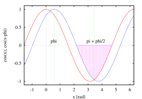
Figure 2: The auxiliary picture to explain the absorption of the impulse carried by TP wave when the phase shift is $\phi$ (see text of Sect. 6.1).

The special assumption of our absorption model was already demonstrated in the last-mentioned figure: if there is more impulse than AP existence, i.e. $|\cos(x)|>|\cos(x-\phi)|$, then the part of the impulse equal to the measure of AP existence, $\cos(x-\phi)$, is absorbed; if the magnitude of AP existence is larger than the actual magnitude of impulse, i.e. $|\cos(x-\phi)|>|\cos(x)|$, then the entire actual impulse, $\cos(x)$, is absorbed. Taking this into account, function $f_{\phi}$, represented by the hatched area in Fig. 2, can be calculated as

$$f_{\phi}=2\int_{\pi/2+\phi}^{\pi+\phi/2}\cos(x-\phi)=-2\left(1-\sin\frac{\phi}{2}\right).$$ (48)

Notice: when $\phi=\pi$, then $f_{\phi}=0$, i.e no impulse is absorbed, therefore the AP does not act on the TP.

In the calculation of integral $f_{\phi}$, we accounted only for the impulse carried by the returning wave, because only this impulse will not be delivered to the TP and, thus, will be missing at the compensation of the impulse from the opposite direction. The size of the incompensated impulse is proportional to $f_{\phi}$, but is delivered to the TP from the opposite side than the site of the absorption of above mentioned returning wave. In the calculation of the acting force, the impulse proportional to the integral $-f_{\phi}$ is thus relevant.

Let us now to calculate the impulse absorbed during the whole time unit interval, $P_{o}$, i.e. the acting force, in fact. This force can be calculated as the integral over the time of impulse $p$, from 0 to $P_{o}$, divided by the period $P_{o}$. Since the proper time integral was already given as the integral $-f_{\phi}$, the acting force can be expressed as

$$F_{act.}=I_{\phi}A_{AP}\frac{4\pi R_{I}^{3}/3}{4\pi r^{2}2R_{I}}M_{o}E_{oR_{I}}.$$ (49)

We denoted $-f_{\phi}/P_{o}=I_{\phi}$.

In the statistics of a large number of particles, the phase shift $\phi$ varies randomly from 0 to $2\pi$. Within our simple model of the absorption, the mean value $<$$I_{\phi}$$>$ of integral $I_{\phi}$ is

$$<I_{\phi}>=\frac{1}{2\pi}\int_{0}^{2\pi}\frac{1}{\pi}\left(1-\sin\frac{\phi}{2}\right)\,d\phi=\frac{1}{\pi}\left(1-\frac{2}{\pi}\right).$$ (50)

6.2 Acting force between macroscopic objects

We already gave the amplitude of the intensity, $E_{or}$, (relation (45)) for $r\ll R_{S}$. In the microcosm, there is no practical use of this formula, since no phenomena are observed in any scale that is many orders of magnitude lower than $\sim$$10^{-15}\,$m. In the microcosm, the amplitude of $E_{or}$ is oscillating, proportional to harmonic functions $\cos(kr)$ and $\sin(kr)$. The concept of the oscillating force seems to be in a disagreement with the behavior of the electric force observed in the macroscopic experiments, where the force is monotonous, either attractive or repulsive, i.e. its sign does not change. This disagreement can, however, be easily explained when we realize that the region of distances $r>|R_{S}|$ is attributed to the atom (i.e. microcosm) and region $r<|R_{S}|$ to the macroscopic phenomena. Namely, the harmonic functions in the formulas for the amplitude, $\cos(kr)$ and $\sin(kr)$, change to the monotonous functions $\cosh(|k|r)$ and $\sinh(|k|r)$ for $r<|R_{S}|$ (implying $|W_{P}/W_{o}|>1$). This is clear from the following analysis of the formula for the magnitude of wave vector (relation (28)). For the particles of the same polarity, $W_{P}>0$, therefore

$$k=\frac{W_{o}}{\hbar c}\sqrt{\frac{-\frac{W_{P}}{W_{o}}}{1+\frac{W_{P}}{W_{o}}}}=i\,\frac{W_{o}}{\hbar c}\sqrt{\frac{\frac{W_{P}}{W_{o}}}{1+\frac{W_{P}}{W_{o}}}}=i|k|.$$ (51)

And, for the particles of opposite polarity with $W_{P}<0$, we can demonstrate that

$$k=\frac{W_{o}}{\hbar c}\sqrt{\frac{-\frac{W_{P}}{W_{o}}}{1+\frac{W_{P}}{W_{o}}}}=\frac{W_{o}}{\hbar c}\sqrt{\frac{\left|\frac{W_{P}}{W_{o}}\right|}{1-\left|\frac{W_{P}}{W_{o}}\right|}}=\frac{W_{o}}{\hbar c}\frac{1}{i}\sqrt{\frac{\left|\frac{W_{P}}{W_{o}}\right|}{\left|\frac{W_{P}}{W_{o}}\right|-1}}=-i|k|.$$ (52)

We now clearly see that $\cos(\pm i|k|r)=\cosh(|k|r)$ and $\sin(\pm i|k|r)=\pm i\,\sinh(|k|r)$.

Because of a larger simplicity and, thus, transparency, we will deal with the Newtonian/Coulombian region of the interaction, further. For $r\ll|R_{S}|$, hence $|W_{P}/W_{o}|\gg 1$, $|k|=W_{o}/(\hbar c)=2\pi m_{o}c/\hbar_{B}=2\pi\omega_{o}/c$ (with a relatively high precision). The explicit form of magnitude of the amplitude $E_{or}$ for $r\ll|R_{S}|$ is

$$|E_{Ar}|=\frac{K_{E}}{r^{2}}\left|\mp i+\frac{2\pi\omega_{o}}{c}r+...\right|\doteq\frac{K_{E}}{r^{2}}.$$ (53)

It means that the amplitude is not only monotonous, but it becomes Newtonian/Coulombian.

At a first glance, it may seem to be strange that the region of distances $r>|R_{S}|$ is regarded as a domain of microscopic phenomena and that with $r\ll|R_{S}|$ as a domain of macroscopic phenomena in classical physics. This apparent paradox can easily be explained, when we realize the consequences of the newly established determination of the generalized Schwarzschild radius. Namely, this radius is $R_{Se}\sim 10^{-15}\,$m for, e.g., the hydrogen atom. However for some macroscopic objects, for example those having the charge $\pm 10^{-9}\,$C, we can found that $R_{S}\sim 10^{5}\,$m. This distance can actually be regarded as much larger than the common laboratory distances of decimetres to metres scale. Term macroscopic thus primarily means a macroscopic number (of charge carriers).

So, let us now to deal with a test object (TO), which consists of a large number of positively charged particles, $N_{+}$, of the same mass $m_{+}$ and large number of negatively charged particles, $N_{-}$, with the same mass $m_{-}$. In a distance $r$ satisfying $r\ll R_{S}$ ($R_{S}$ of the system), let there is situated an acting object (AO) again consisting of a large number of positively charged particles, $n_{+}$, having mass $m_{+}$ and large number of negatively charged particles, $n_{-}$, with mass $m_{-}$. We consider the point-like TO and AO, i.e. their dimensions are much smaller than their mutual distance $r$.

Obviously, the acting force is the appropriate multiple of partial forces acting on the individual particles of the TO, i.e.

$$F_{act.}=\frac{M_{o}K_{E}<I_{\phi}>}{6r^{2}}\left[i\,n_{+}\left(1+\frac{m_{+}^{2}}{2M_{o}^{2}}\right)-i\,n_{-}\left(1+\frac{m_{-}^{2}}{2M_{0}^{2}}\right)+n_{+}\frac{m_{+}}{M_{o}}+n_{-}\frac{m_{-}}{M_{o}}\right].$$

$$.\left[i\,N_{+}\left(1+\frac{m_{+}^{2}}{2M_{o}^{2}}\right)-i\,N_{-}\left(1+\frac{m_{-}^{2}}{2M_{0}^{2}}\right)+N_{+}\frac{m_{+}}{M_{o}}+N_{-}\frac{m_{-}}{M_{o}}\right]$$ (54)

where we already generalized the absorption amplitude, which is also the appropriate multiple of partial absorptions. The last force law can be re-written to form (further, we neglect the terms containing the second power $m^{2}/M_{o}^{2}$)

$$F_{act.}=\frac{M_{o}K_{E}<I_{\phi}>}{6r^{2}}\left[i\,(n_{+}-n_{-})+\frac{n_{+}m_{+}+n_{-}m_{-}}{M_{o}}\right].$$

$$.\left[i\,(N_{+}-N_{-})+\frac{N_{+}m_{+}+N_{-}m_{-}}{M_{o}}\right]=$$

$$=\frac{M_{o}K_{E}<I_{\phi}>}{6r^{2}}\left\{\left[-(n_{+}-n_{-})(N_{+}-N_{-})+\right.\right.$$

$$\left.\left.+\frac{1}{M_{o}^{2}}(n_{+}m_{+}+n_{-}m_{-})(N_{+}m_{+}+N_{-}m_{-})\right]+\right.$$

$$\left.+i\,\frac{1}{M_{o}}\left[(N_{+}-N_{-})(n_{+}m_{+}+n_{-}m_{-})+(n_{+}-n_{-})(N_{+}m_{+}+N_{-}m_{-})\right]\right\}.$$ (55)

In the real world, we assume that only the real component of this force is observed. Therefore, the macroscopic unified acting force can be, finally, written as

$$F_{A}=\frac{M_{o}K_{E}<I_{\phi}>}{6r^{2}}\left[-(n_{+}-n_{-})(N_{+}-N_{-})+\right.$$

$$\left.+\frac{1}{M_{o}^{2}}(n_{+}m_{+}+n_{-}m_{-})(N_{+}m_{+}+N_{-}m_{-})\right].$$ (56)

We note that, usually, $m_{+}\equiv m_{p}$ and $m_{-}\equiv m_{e}$, therefore ratio $m_{\pm}/M_{o}\ll 1$. Despite this circumstance, we keep the term containing the quadrate of this ratio, because the first term may be zero, when $n_{+}=n_{-}$ or $N_{+}=N_{-}$.

The analysis of force $F_{A}$ yields the following conclusions.
(1) Two objects charged with the charges of the same polarity, i.e. $n_{+}>n_{-}$ and $N_{+}>N_{-}$ (or $n_{+}<n_{-}$ and $N_{+}<N_{-}$): the first term, which we starts to refer to as ,,the first electric-force term”, is $-(n_{+}-n_{-})(N_{+}-N_{-})<0$. On contrary, the term $(n_{+}m_{+}+n_{-}m_{-})(N_{+}m_{+}+N_{-}m_{-})/M_{o}^{2}$, which we will refer to as ,,the secondary electric-force term”, is positive. Therefore the orientation of the secondary electric force is opposite with respect to the orientation of the first-term, dominant electric force. We note that the secondary electric force is $\sim$$m^{2}/M_{o}^{2}\sim 10^{-36}$ times smaller, when $m_{+}\equiv m_{p}$ and $m_{-}\equiv m_{e}$.
(2) Two objects charged with the charges of the opposite polarity, i.e. $n_{+}>n_{-}$ and $N_{+}<N_{-}$ (or $n_{+}<n_{-}$ and $N_{+}>N_{-}$): the first electric-force term, $-(n_{+}-n_{-})(N_{+}-N_{-})$ is larger than zero, this time. The secondary electric-force term, $(n_{+}m_{+}+n_{-}m_{-})(N_{+}m_{+}+N_{-}m_{-})/M_{o}^{2}$, remains positive. Therefore the orientation of the secondary electric force is the same as the orientation of the first-term electric force.
(3) The charged TO and electrically neutral AO (or vice versa), i.e. $n_{+}\neq n_{-}$ and $N_{+}=N_{-}$ (or $n_{+}=n_{-}$ and $N_{+}\neq N_{-}$): the first electric-force term, $-(n_{+}-n_{-})(N_{+}-N_{-})$ is zero. However, the secondary electric-force term, $(n_{+}m_{+}+n_{-}m_{-})(N_{+}m_{+}+N_{-}m_{-})/M_{o}^{2}$, remains the same size and positive as in the previous cases. There is no first-term electric force acting, but the secondary electric force is not influenced with the electric charge of whatever of the two objects.
(4) Two electrically neutral objects, i.e. $n_{+}=n_{-}$ and $N_{+}=N_{-}$: the first electric-force term, $-(n_{+}-n_{-})(N_{+}-N_{-})$ is zero as expected. However, the secondary electric-force term, $(n_{+}m_{+}+n_{-}m_{-})(N_{+}m_{+}+N_{-}m_{-})/M_{o}^{2}$, remains the same size and positive even in this case. Again, there is no first-term electric force acting, but the secondary electric force is, as we could see, always ,,surviving”.

We can see that the nominator of the secondary electric-force term, $(n_{+}m_{+}+n_{-}m_{-})(N_{+}m_{+}+N_{-}m_{-})$, is, in fact, the product of multiplication of the masses, $n_{+}m_{+}+n_{-}m_{-}$ and $N_{+}m_{+}+N_{-}m_{-}$, of the AO and TO, respectively. While the primary electric force is proportional to unity (constant) and cannot depend on the curvature of space-time or velocity of the object (in the sense as the mass depends on the curvature and/or velocity according $m=m_{o}/\sqrt{g_{44}}$), the secondary electric force does so.

The revealed secondary electric force has all attributes to be identified to the gravitational force.

We formally assign the cosine (hyperbolic cosine) part of the electric-intensity amplitude to the electric part (electric charge) of the unified interaction and sine (hyperbolic sine) part to the gravitational part (mass) of the interaction.

6.3 Net electric charge of stars

There is a case when the second power of ratio $m/M_{o}$ is not negligible in the unified force law (in the parentheses of relation (6.2)). Let us to consider the TP consisting of a single electron and a large macroscopic body (as the AO) consisting of the same number, $n_{+}$, of protons and electrons, $n_{-}$ ($n_{+}=n_{-}$), e.g. a pure-hydrogen star. The absorption amplitude is

$$A_{AO}=n_{+}\,i\,\left(1+\frac{m_{p}^{2}}{2M_{o}^{2}}\right)+n_{-}(-i)\left(1+\frac{m_{e}^{2}}{2M_{o}^{2}}\right)+$$

$$+n_{+}\frac{m_{p}}{M_{o}}+n_{-}\frac{m_{e}}{M_{o}}=i\,n_{+}\frac{m_{p}^{2}-m_{e}^{2}}{2M_{o}^{2}}+n_{+}\frac{m_{p}+m_{e}}{M_{o}}.$$ (57)

The acting force in this system is

$$F_{act.}=\frac{M_{o}K_{E}<I_{\phi}>}{6r^{2}}A_{AO}\left(-i+\frac{m_{e}}{M_{o}}\right)$$ (58)

and its component in the real space, the effect of which is observable, can be obtained, after the product $A_{AO}$ and parentheses is calculated, as

$$F_{A,real}=\frac{M_{o}K_{E}<I_{\phi}>}{6r^{2}}\left(n_{+}\frac{m_{p}^{2}-m_{e}^{2}}{2M_{o}^{2}}+n_{+}\frac{m_{p}+m_{e}}{M_{o}}\frac{m_{e}}{M_{o}}\right).$$ (59)

The third electric-force term (it is written as the first term in the parentheses) is, here, greater than the secondary (gravitational) term.

Specifically, the ratio is

$$\frac{n_{+}\frac{m_{p}^{2}-m_{e}^{2}}{2M_{o}^{2}}}{n_{+}(m_{p}+m_{e})\frac{m_{e}}{M_{o}^{2}}}=\frac{m_{p}-m_{e}}{2m_{e}}\doteq\frac{1}{2}\frac{m_{p}}{m_{e}}\doteq 918.$$ (60)

The third electric-force term is the term of the electric part (hyperbolic cosine) of the unified force. The above derived force is the electric force between the net charge of the macroscopic body and the charge of electron.

The net electrostatic field of the Sun and other stars was found within the old model of solar atmosphere by Dutch astronomer Pannekoek (1922) and generalized as the attribute of the whole solar/stellar body, not only of atmosphere, by Rosseland (1924). The field was studied till the middle of 19-ty fifties by several astrophysicists (e.g. Eddington, 1926; Cowling, 1929; Pikel’ner, 1948; 1950; van de Hulst, 1950; 1953). It was mainly linked, in the minds of experts, to the models of the solar corona. It seems that it was later forgotten together with the obsolete models of the corona, when these models were replaced by the MHD models. The principle of the generation of this field is, however, not exclusively related to any stellar atmosphere. The lighter and thus faster moving electrons tend to separate from the heavier protons (ions) in the stellar plasma. If the Sun was electrically neutral, $22\%$ of all electrons on its surface would reach the escape velocity (in contrast to only $10^{-1735}\%$ of protons). When the field acts on an electron, the electric force is actually $m_{p}/(2m_{e})\doteq 918$ times stronger than the gravity, as we found.

The Pannekoek-Rosseland electric field equalizes the probability of the escape of both polarity charge-carriers away from a star. The field can be expressed in form of the net charge of star (Neslušan, 2001). This charge is positive and within the sphere of radius $r$ equals

$$Q_{r}=\frac{2\pi\varepsilon_{o}\kappa(m_{p}-m_{e})}{q_{o}}M_{r},$$ (61)

where $M_{r}$ is the stellar mass within the radius $r$. When the third term of the acting unified force is re-written with the help of product of charges of electron and macroscopic body, we obtain the charge of the body identical to the Pannekoek-Rosseland charge (61).

In the representation when the magnitudes of positive and negative elementary electric charges are exactly the same, the net charge of star can occur due to the asymmetry of the numbers of carriers of both kinds. In our concept of unified force and, consequently, the unified concept of charge and mass, the elementary charge slightly depends on the mass of its carrier, therefore the magnitude of the charge of proton is slightly larger than that of electron. In this concept, the Pannekoek-Rosseland net charge occurs at exactly the same number of carriers of both positive and negative charges. In the new concept, the symmetry of the magnitudes of positive and negative elementary charge is replaced with the symmetry of their numbers.

6.4 Acting force in microcosm

Let us again to consider the proton-electron system. To give the force acting on the electron in this system, we use the originally derived relation for the electric intensity (42), so called standard solution, $E_{or}\propto\sqrt{k_{+}/k_{-}}\cos(kr)-i\,\sin(kr)$. The corresponding force is

$$F_{A,micro}=A_{AP}\frac{M_{o}K_{E}}{6r^{2}}\left[\sqrt{\frac{k_{+}}{k_{-}}}\cos(kr)-i\,\sin(kr)\right],$$ (62)

where the absorption amplitude $A_{AP}$ is the same as in the case of macroscopic interaction (relation (46)) since the proton absorbes the impulse carried by the wave associated with the electron with the maximum screening radius equal to $R_{I}$. With this amplitude, i.e. with $A_{AP}=i+m_{p}/M_{o}$, we can derive

$$F_{A,micro}=\frac{M_{o}K_{E}}{6r^{2}}\left\{\left[\sin(kr)+\frac{m_{p}}{M_{o}}\sqrt{\frac{k_{+}}{k_{-}}}\cos(kr)\right]+\right.$$

$$\left.+i\,\left[\sqrt{\frac{k_{+}}{k_{-}}}\cos(kr)-\frac{m_{p}}{M_{o}}\sin(kr)\right]\right\}.$$ (63)

Its real componet, which is manifested in the observed world, is

$$F_{A,micro}=\frac{M_{o}K_{E}}{6r^{2}}\left[\sin(kr)+\frac{m_{p}}{M_{o}}\sqrt{\frac{k_{+}}{k_{-}}}\cos(kr)\right].$$ (64)

In the atom shell, where $r\approx R_{S}/\alpha_{B}^{2}$, it is valid $(m_{p}/M_{o})\sqrt{k_{+}/k_{-}}\approx m_{p}/(\alpha_{B}M_{o})\ll 1$. So, the second term can well be neglected, therefore the force becomes proportional only to the function of $\sin(kr)$, i.e.

$$F_{A,real}=\frac{M_{o}K_{E}}{6r^{2}}\sin(kr).$$ (65)

The behavior of $F_{A,real}$ (zero-force distances) is illustrated in Fig. 3.

Figure 3: The dependence of the real-valued amplitude of radial component of the electric force, $F_{A,real}$, in the hydrogen atom on distance $r$ from the central proton. The behavior is illustrated for $l=0$ in the region of the atomic shell (scale $r_{B}=R_{Se}/\alpha_{B}^{2}$). The repulsive force corresponds with $F_{A,real}>0$ and attractive force with $F_{A,real}<0$.

From relation (65), it is clear that the stable-equilibrium ZFDs, $r_{0n}$, satisfy condition $kr_{0n}=2\pi n$, where $n$ is a positive integer. In fact, number $n$ is an analogue of the main quantum number in the classical-quantum-mechanics description of hydrogen atom.

The magnitude of the wave vector, $k$, is given by relation (28) in the general case, or can be written as

$$k=\frac{2\pi\alpha_{B}}{R_{Se}}\sqrt{\frac{\frac{R_{Se}}{r}}{1-\frac{R_{Se}}{r}}},$$ (66)

for the proton-electron system. Supplying $k$ into the condition $kr_{0n}=2\pi n$ for the ZFDs, we can re-write this condition to the quadratic equation

$$\frac{\alpha_{B}^{2}}{n^{2}}\left(\frac{r_{0n}}{R_{Se}}\right)^{2}-\frac{r_{0n}}{R_{Se}}+1=0$$ (67)

having the solution

$$r_{0n}=\left(1\pm\sqrt{1-4\alpha_{B}^{2}/n^{2}}\right)\frac{n^{2}}{2\alpha_{B}^{2}}R_{Se}.$$ (68)

The first group of $r_{0n}$, with plus sign in front of the square root in (68), corresponds to the stable-equilibrium ZFDs of the electron in the atomic shell.

Using relation $W=\sqrt{\hbar^{2}c^{2}k^{2}+W_{o}^{2}}+W_{P}$ (identical to $W=W_{o}/\sqrt{g_{44}}+W_{P}$) for the energy, $W$, in which we supply $W_{P}=-W_{o}R_{Se}/r$, energy $W$ can be re-written as

$$W=W_{o}\left(\frac{1}{\sqrt{1-R_{Se}/r_{12}}}-\frac{R_{Se}}{r_{12}}\right),$$ (69)

where $r_{12}=(1+m_{oe}/m_{op})r$ includes the correction for the barycenter of the system ($m_{oe}$ and $m_{op}$ are the rest masses of electron and proton, respectively). The energy terms can be calculated supplying $r=r_{0n}$. The obtained enegry terms are identical to those characterized with $l_{D}=n_{D}-1$ and $j_{D}=l_{D}+1/2$ in the Dirac’s solution. (Unfortunately, the full set of energy levels is not known within the presented implicit-$k$ solution of MEs. It can likely be obtained after the generalization of the universal metrique towards the axial-symmetry, e.g. Kerr solution of Einstein field equations and after the full solution of the MEs, with also $E_{\vartheta}$ and $E_{\varphi}$ components of the electric-intesity vector found.) The comparison of our result to the terms predicted according the Dirac’s theory as well as to the experimental values is given in Table 2.

Table 2: The ZFDs, $r_{0n}$, and corresponding energetic excesses over the rest energy, $W-W_{o}$, for several first values of $n$ as calculated by the solution for $F_{A,real.}$. The corresponding energetic terms, $W_{D}$, calculated according the Dirac’s theory with the appropriate main quantum number, $n_{D}$, orbital quantum number, $l_{D}$, and spin-orbital quantum number, $j_{D}$, as well as the experimental terms, $W_{\rm exp.}$, are given, too.

$n$	$r_{0n}$	$W-W_{o}$	$n_{D}$	$l_{D}$	$j_{D}$	$W_{D}$	$W_{\rm exp.}$
	$[r_{B}]$	$[eV]$				$[eV]$	$[eV]$
$1$	0.9999468	$-13.598474$	1	0	1/2	$-13.598474$	$-13.598439$
$2$	3.9999467	$-3.3995845$	2	1	3/2	$-3.3995845$	$-3.3995843$
$3$	8.9999468	$-1.5109237$	3	2	5/2	$-1.5109237$	$-1.5109236$
$4$	15.999948	$-0.849894$	4	3	7/2	$-0.849894$	$-0.849894$

When we consider the sign minus in the relation (68) for $r_{0n}$, we gain another, second group of the ZFDs. In this case, $r_{0n}$ can be approximated as

$$r_{0n}=R_{Se}\left(1+\frac{\alpha_{B}^{2}}{n^{2}}+...\right)\doteq R_{Se}.$$ (70)

We clearly see that these ZDFs are closely above the generalized Schwarzschild’s radius, at distances $\approx 10^{-15}\,$m. These ZFDs provide us with a possibility to explain, on the basis of electric interaction, the quantization in the atomic nucleus. The behavior of the oscillating force at the Schwarzschild’s radius is shown in Fig. 4.

The possible identity of the strong force with the electric one can also be supported by the following estimate of energy. In a much larger or a much smaller distance $r$ than $R_{S}$ (in the case of atom, in the atom shell), the magnitude of free energy, $|W-W_{o}|=|W_{o}/\sqrt{|1-R_{S}/r|}-W_{o}R_{S}/r|$, is of order $|W-W_{o}|\sim W_{o}R_{S}/r$, i.e. its behavior is Newtonian/Coulombian. We remind that the energy of radiation (of an emitted photon) can originate, in atom, from the difference $W-W_{o}$. At the nucleus, $r\rightarrow R_{Se}$ and we can show that the magnitude of free energy is of order $\sim$$W_{o}/\alpha_{B}$. Since the corresponding Newtonian/Coulombian free energy would be of order $\sim$$W_{o}R_{Se}/R_{Se}\sim W_{o}$, it is clear that the actual free energy, $W-W_{o}$, is about the factor of $1/\alpha_{B}\sim 10^{2}$ higher at the nucleus in comparison with Coulombian behavior.

Figure 4: The dependence of the real-valued amplitude of radial component of the electric force, $F_{A,real}$, in the hydrogen atom on distance $r$ from the central proton. In this plot, the behavior is illustrated in the region close above the generalized Schwarzschild radius, $R_{Se}$. Force is given in arbitrary units which, however, correspond to those used in Fig. 3.

It seems that the old concept of the neutron as the particle composed of proton and electron becomes again actual. In principle, the energy excess between the rest energy of neutron and sum of proton+electron mass could be predicted, here. As well, the nuclear systems consisting of several protons and neutrons (neutrons as protons+electrons) seems possible to be explained. Unfortunately, an usage of our concept for quantitative calculations appears to be difficult, because it is not longer valid that $r\gg R_{Se}$ (as in atomic shell), therefore the particles cannot be regarded as point-like objects and, especially, the dependence of the potential energy on the distance $r$ is not known. The common Coulomb approximation is absolutely inappropriate in this ultra-relativistic region.

At last, we can explain why the ,,strong force” (electrical, in fact) does not oscillate and, thus, does not create the stable systems between two protons (why there is no proton-proton bound pair). The potential energy of a proton in the electric force field of another proton is positive, therefore the amplitude of the wave vector, in this case, is

$$k=\frac{2\pi\alpha_{B}}{R_{Sp}}\sqrt{\frac{-\frac{R_{Sp}}{r}}{1+\frac{R_{Sp}}{r}}}=i\,\frac{2\pi\alpha_{B}}{R_{Sp}}\sqrt{\frac{\frac{R_{Sp}}{r}}{1+\frac{R_{Sp}}{r}}}=i|k|,$$ (71)

where $R_{Sp}$ is the generalized Schwarzschild radius for the proton-proton system. Therefore, the argument of the functions of cosine and sine, $kr$, is changed to $i|k|r$. Consequently, the amplitude of the standard solution now is

$$E_{A,pp}=\frac{K_{E}}{r^{2}}\left[\sqrt{\frac{k_{+}}{k_{-}}}\cosh(|k|r)+\sinh(|k|r)\right].$$ (72)

Both hyperbolic cosine and hyperbolic sine are monotonous functions, which yield no ZFD.

Finding the stable-equilibrium ZFDs, we create, in fact, the concept of the atom, in which the electrons in its shell and, probably, the nucleons in its nucleus are not orbiting the center of the system, but all these particles are in the rest in the ZFDs. An essential feature of the concept is the electric force changing its magnitude and sign with the radial distance from the center of the system, i.e. the oscillating force.

7 Inertia force

If a particle is in the rest or moves with a constant velocity, its associated wave is perfectly spherically symmetric and the particle is exactly in the wave center. The impulse, carried by this wave, is completely compensated when the wave leaves or impacts the particle, as already mentioned.

However, if the particle accelerates (see scheme in Fig. 5), the wave in the direction of the acceleration is blue-shifted, its frequency increases and, consequently, the impulse becomes larger in this direction. In the opposite direction, the wave is red-shifted and corresponding impulse reduced. The impulse coming from the direction of the acceleration of particle is not longer completely compensated by the impulse from the opposite direction $-$ there occurs a force acting on the particle. This mechanism is the nature of the inertia force.

Figure 5: The impulse carried by the wave associated with the particle (full bullet) when the particles accelerates (1D case). This time, the impulse is not completely compensated ($p_{1}<p_{2}$ because $\lambda_{1}>\lambda_{2}$).

The angular frequency of the wave spreading in the direction declined by the angle $\vartheta$ from the direction of the acceleration is

$$\omega_{o}=\frac{\omega_{oc}}{1-(\Delta v/c)\cos\vartheta},$$ (73)

where $\omega_{oc}$ is the angular frequency of the particle in rest and in free space and $\Delta v$ is the change of the velocity of particle during a time interval. We identify this interval to the unit interval of time, $P_{o}$.

The impulse carried by the wave in the direction characterized by common spherical angles $\varphi$ and $\vartheta$ at the distance of interaction radius, $R_{I}$, which crosses the infinitesimal area $R_{I}^{2}\sin\vartheta\,d\varphi\,d\vartheta$ within the time interval $dt$, according the standard solution, is

$$d^{3}p(\varphi,\vartheta)=\frac{R_{I}^{2}\sin\vartheta\,d\varphi\,d\vartheta}{4\pi R_{I}^{2}}\frac{M_{o}K_{E}}{R_{I}^{2}}\left[\mp i\,\cosh\left(\frac{2\pi\omega_{o}R_{I}}{c}\right)+\right.$$

$$\left.+\sinh\left(\frac{2\pi\omega_{o}R_{I}}{c}\right)\right]\cos(2\pi\Omega t)\,dt.$$ (74)

In the last relation, we consider only the cosine part of the function $\exp(-i2\pi\Omega t)$ describing the wave in the real-valued space (just this part was also considered at the derivation of acting force).

The component of the impulse delivered to the particle in the direction opposite to its acceleration obviously is $d^{3}p(\varphi)=\cos\vartheta\,d^{3}p(\varphi,\vartheta)$ (see Fig. 6). The sum of the impulse over all values of $\varphi$, i.e. from the circle inclined by angle $\vartheta$ to the aceleration direction, is $d^{2}p=2\pi d^{3}p(\varphi,\vartheta)$.

Figure 6: The impulse carried by the wave associated with the particle: its fraction $\vec{p}$ in the direction characterized by the angles $\varphi$ and $\vartheta$ and the component of this impulse $p_{z}$ in the direction of the particle acceleration.

The inertia force is double integral of impulse $d^{2}p$ over all values of angle $\vartheta$ and over the whole period of the particle oscillation divided by this period, i.e.

$$F_{iner.}=-\frac{1}{P_{o}}\int_{0}^{P_{o}}\int_{0}^{\pi}\frac{2\pi R_{I}^{2}}{4\pi R_{I}^{2}}\frac{M_{o}K_{E}}{R_{I}^{2}}\left[\mp i\,\cosh\left(\frac{2\pi R_{I}}{c}\frac{\omega_{oc}}{1-(\Delta v/c)\cos\vartheta}\right)+\right.$$

$$\left.+\sinh\left(\frac{2\pi R_{I}}{c}\frac{\omega_{oc}}{1-(\Delta v/c)\cos\vartheta}\right)\right]\cos\vartheta\sin\vartheta\,d\vartheta\,|\cos(2\pi\Omega t)|\,dt.$$ (75)

We add the sign minus to respect the fact that the impulse delivered to the considered particle has the opposite direction than the acceleration of the particle.

If the wave impacts the particle, it gives the carried impulse in the direction of its motion; if the wave leaves the particle, the impulse is again given in this direction due to the action-reaction principle. This fact is respected taking the absolute value $|\cos(2\pi\Omega t)|$ in the calculation of $F_{iner.}$. If we denote

$$I_{t}=\frac{1}{P_{o}}\int_{0}^{P_{o}}|\cos(2\pi\Omega t)|\,dt=\frac{2}{\pi},$$ (76)

then the force can be given as

$$F_{iner.}=-\frac{M_{o}K_{E}I_{t}}{2R_{I}^{2}}\int_{0}^{\pi}\left[\mp i\,\cosh\left(\frac{2\pi R_{I}}{c}\frac{\omega_{oc}}{1-(\Delta v/c)\cos\vartheta}\right)+\right.$$

$$\left.+\sinh\left(\frac{2\pi R_{I}}{c}\frac{\omega_{oc}}{1-(\Delta v/c)\cos\vartheta}\right)\right]\cos\vartheta\sin\vartheta\,d\vartheta.$$ (77)

Integral

$$I_{\vartheta}=\int_{0}^{\pi}\left[\mp i\,\cosh\left(\frac{2\pi R_{I}}{c}\frac{\omega_{oc}}{1-(\Delta v/c)\cos\vartheta}\right)+\right.$$

$$\left.+\sinh\left(\frac{2\pi R_{I}}{c}\frac{\omega_{oc}}{1-(\Delta v/c)\cos\vartheta}\right)\right]\cos\vartheta\sin\vartheta\,d\vartheta$$ (78)

can be calculated after we develop the functions hyperbolic cosine and hyperbolic sine into the power series. The result of integration is

$$I_{\vartheta}=\pm i\,\left[S^{2}\sum_{j=1}^{\infty}\frac{2j}{2j+1}\left(\frac{\Delta v}{c}\right)^{2j-1}+\right.$$

$$\left.+4\sum_{s=1}^{\infty}\frac{S^{2s}}{(2s)!(2s-1)!}\sum_{j=1}^{\infty}\frac{j(2s+2j-2)!}{(2j+1)!}\left(\frac{\Delta v}{c}\right)^{2j-1}\right]+$$

$$+\left[2S\sum_{j=1}^{\infty}\frac{1}{2j+1}\left(\frac{\Delta v}{c}\right)^{2j-1}+\right.$$

$$\left.+4\sum_{s=1}^{\infty}\frac{S^{2s-1}}{(2s-1)!(2s-2)!}\sum_{j=1}^{\infty}\frac{j(2s+2j-3)!}{(2j+1)!}\left(\frac{\Delta v}{c}\right)^{2j-1}\right],$$ (79)

where we used denotation $S=2\pi\omega_{oc}R_{I}/c=m_{oc}/M_{o}$.

We can demonstrate that the power series in the result of integral $I_{\vartheta}$ are convergent for $\Delta v/c<1$. Condition $\Delta v/c<1$ sets the maximum possible acceleration of the particle (i.e. maximum increment, $\Delta v$, acquired during the period $P_{o}$) in the universe.

Since $S=m_{oc}/M_{o}\ll 1$, usually, we can neglect higher powers of $S$. As well, the common accelerations, $\Delta v$ within the period $P_{o}$, are many orders of magnitude smaller than the speed of light, $c$, therefore we can also neglect higher powers of $\Delta v/c$. Integral $I_{\vartheta}$ for the all known situations in the universe can be written in the simple form

$$I_{\vartheta}=\frac{2}{3}\frac{m_{oc}}{M_{o}}\left(\frac{\Delta v}{c}\right)+\frac{2}{5}\frac{m_{oc}}{M_{o}}\left(\frac{\Delta v}{c}\right)^{3}+...\pm i\,\left[\frac{2}{3}\frac{m_{oc}^{2}}{M_{o}^{2}}\left(\frac{\Delta v}{c}\right)+...\right].$$ (80)

Since we observe only the phenomena manifestating themselves in the real space, it is reasonable, also here, to consider only the real component of $I_{\vartheta}$, where the second term containing $(\Delta v/c)^{3}$ can influence the size of inertia force in, e.g., an extreme deceleration of a particle striking a high potential barrier. In the common physics, it is enough to consider only the first term of the real component, with which the inertia force is

$$F_{iner.}=-\frac{M_{o}K_{E}I_{t}}{3R_{I}^{2}}\frac{m_{oc}}{M_{o}}\frac{\Delta v}{c}.$$ (81)

REMARK. Notice that the imaginary part of integral $I_{\vartheta}$, which corresponds to the hyperbolic cosine and, hence, the electric part of the unified force, starts with the term contaning the second power of $m_{oc}/M_{o}$. Actually, the integral of the first term is

$$I_{\vartheta,i1}=\int_{0}^{\pi}(\pm i)\,\cos\vartheta\,\sin\vartheta\,d\vartheta=0.$$ (82)

This result explains why the inertia force is proportional to the mass of bodies, but it is not proportional to the electric charge $[$even if the electric part $\pm\cosh(m_{oc}/M_{o})$ would be re-scalled, in an alternative solution, to be real-valued$]$. We note that typically $m_{oc}/M_{o}\approx 10^{-18}$, therefore the electric ,,inertia term”, $m_{oc}^{2}/M_{o}^{2}$, is about 18 orders of magnitude smaller than the gravitational inertia term, $m_{oc}/M_{o}$.

The acceleration uses to be given in the form of $\Delta v/\Delta t$. We said that the time interval, $\Delta t$, equals $\Delta t=P_{o}=\hbar_{B}/(\pi M_{o}c^{2})$ in our case. So, we can re-write the ratio $\Delta v/c$ as $(\Delta v/\Delta t)(\Delta t/c)=[\hbar_{B}/(\pi M_{o}c^{3})](\Delta v/\Delta t)$. Using the latter, the inertia force (its real component) can be given in the more familiar form as

$$F_{iner.}=-\frac{\hbar_{B}M_{o}K_{E}}{3\pi}\frac{I_{t}}{R_{I}^{2}M_{o}^{2}c^{3}}m_{oc}\frac{\Delta v}{\Delta t}.$$ (83)

The inertia force of an object consisting of $N_{+}$ positively charged particles having the mass $m_{+}$ and $N_{-}$ negatively charged particles having the mass $m_{-}$ is simply the sum of partial inertia forces of all constituent particles, i.e.

$$F_{iner.}=-\frac{M_{o}K_{E}}{3\pi}\frac{\hbar_{B}I_{t}}{R_{I}^{2}M_{o}^{2}c^{3}}(N_{+}m_{+}+N_{-}m_{-})\frac{\Delta v}{\Delta t}.$$ (84)

8 Equation of motion

8.1 Equation of motion in traditional form

In two sections avove, the acting and inertia forces were derived in forms different from those in the Coulomb and Newton laws. In this subsection, we show that our result is consistent with the conventional equations of motion containing the Coulomb and Newton laws despite the difference.

The inertia and acting forces should be equal in a description of motion of a body. Let us now to consider the macroscopic test body being in rest in the distance $r$ from another body, whereby the sizes of both bodies are negligible in respect to the distance $r$. The equation of motion of the test body, based on our derivations of acting and inertia forces, is

$$-\frac{M_{o}K_{E}}{3\pi}\frac{\hbar_{B}I_{t}}{R_{I}^{2}M_{o}^{2}c^{3}}(N_{+}m_{+}+N_{-}m_{-})\frac{\Delta v}{\Delta t}=$$

$$=\frac{M_{o}K_{E}<I_{\phi}>}{6r^{2}}\left[-(n_{+}-n_{-})(N_{+}-N_{-})+\right.$$

$$\left.+\frac{1}{M_{o}^{2}}(n_{+}m_{+}+n_{-}m_{-})(N_{+}m_{+}+N_{-}m_{-})\right].$$ (85)

The forms $N_{+}m_{+}+N_{-}m_{-}$ and $n_{+}m_{+}+n_{-}m_{-}$ are, in fact, the masses of the test object and acting object, which we denote by $\tilde{m}_{T}$ and $\tilde{m}_{A}$, respectively. The forms $(N_{+}-N_{-})M_{o}$ and $(n_{+}-n_{-})M_{o}$ can be given as $(N_{+}-N_{-})q_{o}/\sqrt{4\pi\varepsilon_{o}\kappa}$ and $(n_{+}-n_{-})q_{o}/\sqrt{4\pi\varepsilon_{o}\kappa}$. (We remind that the elementary electromass $M_{o}=q_{o}/\sqrt{4\pi\varepsilon_{o}\kappa}$.) Further, we denote $\tilde{q}_{T}=(N_{+}-N_{-})q_{o}$ and $\tilde{q}_{A}=(n_{+}-n_{-})q_{o}$, whereby $\tilde{q}_{T}$ and $\tilde{q}_{A}$ are the electric charges of the test object and acting object, respectively. The fine structure constant, $\alpha_{B}$, can be given with the help of the gravitational constant, $\kappa$, elementary electromass, $M_{o}$, Planck’s constant divided by $2\pi$, and velocity of light, $c$, as $\alpha_{B}=\kappa M_{o}^{2}/(\hbar_{B}c)$.

After some handling, the equation of motion (8.1) can be re-written into the form

$$\tilde{m}_{T}\frac{\Delta v}{\Delta t}=\frac{<I_{\phi}>}{8\pi I_{t}}\frac{1}{\alpha_{B}}\left[\frac{\tilde{q}_{T}\tilde{q}_{A}}{4\pi\varepsilon_{o}r^{2}}-\kappa\frac{\tilde{m}_{T}\tilde{m}_{A}}{r^{2}}\right].$$ (86)

If

$$\frac{<I_{\phi}>}{8\pi I_{t}}\frac{1}{\alpha_{B}}=1,$$ (87)

we obtain the unified equation of motion in the classical physics. In more detail, if the charges $\tilde{q}_{T}$ and $\tilde{q}_{A}$ are not zero, we can neglect the second term in the brackets and the equation becomes

$$\tilde{m}_{T}\frac{\Delta v}{\Delta t}=\frac{\tilde{q}_{T}\tilde{q}_{A}}{4\pi\varepsilon_{o}r^{2}}.$$ (88)

We can clearly see that it is the classical equation of motion for two charged objects.

If at least one charge is zero, then the first term in the brackets of eq.(86) is zero and only the second term remains. So, the equation, in this case, is

$$\tilde{m}_{T}\frac{\Delta v}{\Delta t}=-\kappa\frac{\tilde{m}_{T}\tilde{m}_{A}}{r^{2}}.$$ (89)

It is nothing else than the classical equation of motion for two gravitationally interacting objects.

The condition (87), i.e. $<$$I_{\phi}$$>$$(1/\alpha_{B})/(8\pi I_{t})=1$, provides us with a possibility to calculate the fine structure constant, if the perfect model of the interaction is known. Specifically,

$$\alpha_{B}=\frac{<I_{\phi}>}{8\pi I_{t}}.$$ (90)

Or, the condition can be used to verify the correctness of the interaction models in future studies. In our simple model of the impulse absorption, with $<$$I_{\phi}$$>=(1-2/\pi)/\pi$ and $I_{t}=2/\pi$, we obtain $\alpha_{Bcalc.}=(1-2/\pi)/(16\pi)=1/138.327511$. It is the value about $1\%$ different from the actual experimental value of $\alpha_{B}=1/(137.035990\pm 0.000006)$.

8.2 Equation of motion in pure-geometrical form

The scientists who created the theory of relativity had an ambition to work out the pure geometrical theory. It means that the equations within this theory would be dimensionless. Our consistent derivation of both acting and inertia forces allows us to achieve this goal, at least in the case of the elementary equation of motion.

In the absolutely autonomous description of a geometric structure, the size of a given feature can be expressed, only, as a relative multiple of the size of other feature. Or, we must choose a unit of length, if we wish to speak about specific value of the size. If the geometric structure is dynamical, changing shapes, sizes, and positions of the features, we can again express the rate of a given change as a relative multiple of the rate of other change. Or, we can do this with establishing the definition of the unit of change. Therefore, two units (relative or established to be ,,absolute”) are necessary, in principle, in the description of pure geometrical, dynamical structure: unit of the length and unit of the rate of its change.

Let us to consider again the inertia force (81), in which we generalize mass $m_{oc}$ to the mass of a macroscopic object, i.e. we replace $m_{oc}\rightarrow N_{+}m_{+}+N_{-}m_{-}$. Putting this force into the equality with the acting force in form (6.2), we obtain the primary form of the equation of motion:

$$-\frac{M_{o}K_{E}}{3R_{I}^{2}}\frac{N_{+}m_{+}+N_{-}m_{-}}{M_{o}}\frac{\Delta v}{c}=$$

$$=\frac{M_{o}K_{E}<I_{\phi}>}{6r^{2}}\left[-(n_{+}-n_{-})(N_{+}-N_{-})+\right.$$

$$\left.+\frac{1}{M_{o}^{2}}(n_{+}m_{+}+n_{-}m_{-})(N_{+}m_{+}+N_{-}m_{-})\right],$$ (91)

which can easily be simplified to

$$\left(N_{+}\frac{m_{+}}{M_{o}}+N_{-}\frac{m_{-}}{M_{o}}\right)\frac{\Delta v}{c}=\frac{<I_{\phi}>}{2I_{t}}\left(\frac{R_{I}}{r}\right)^{2}\left[(n_{+}-n_{-})(N_{+}-N_{-})+\right.$$

$$\left.-\left(n_{+}\frac{m_{+}}{M_{o}}+n_{-}\frac{m_{-}}{M_{o}}\right)\left(N_{+}\frac{m_{+}}{M_{o}}+N_{-}\frac{m_{-}}{M_{o}}\right)\right].$$ (92)

We derived this equation using the same initial formulas as in the derivation of eq.(86). Only a difference in algebraic operations was sufficient to eliminate the constants as gravitational constant or permitivity of vacuum. Notice further that eq.(8.2) is dimensionless: only the dimensionless numbers of particles, dimensionless integrals, and ratios of masses, velocities, and distances figure there.

In eq.(8.2), the masses $m_{+}$ and $m_{-}$ can be re-written with the help of the well-known de Broglie’s relation as $m_{+}=h_{B}\tilde{\nu}_{+}/c^{2}$ and $m_{-}=h_{B}\tilde{\nu}_{-}/c^{2}$, where $\tilde{\nu}_{+}$ and $\tilde{\nu}_{-}$ are the frequencies of the waves associated with the particles of masses $m_{+}$ and $m_{-}$, respectively. As well, we establish the frequency $\nu_{o}$ associated with the wave corresponding to the elementary electromass, $M_{o}$, whereby $M_{o}=h_{B}\nu_{o}/c^{2}$. Or, the frequencies can be replaced with the corresponding wavelengths when we use relations $\tilde{\nu}_{+}=c/\tilde{\lambda}_{+}$, $\tilde{\nu}_{-}=c/\tilde{\lambda}_{-}$, and $\nu_{o}=c/\Lambda_{C}$. The ratio of integrals $<$$I_{\phi}$$>$$/I_{t}$ can be given with the help of relation (87) as $<$$I_{\phi}$$>$$/I_{t}=8\pi\alpha_{B}$. Using the above mentioned relations and after few algebraic operations, the equation (8.2) can be re-written into the form

$$\left(N_{+}\frac{\Lambda_{C}}{\tilde{\lambda}_{+}}+N_{-}\frac{\Lambda_{C}}{\tilde{\lambda}_{-}}\right)\frac{\Delta v}{c}=4\pi\alpha_{B}\left(\frac{R_{I}}{r}\right)^{2}\left[(n_{+}-n_{-})(N_{+}-N_{-})-\right.$$

$$\left.-\left(n_{+}\frac{\Lambda_{C}}{\tilde{\lambda}_{+}}+n_{-}\frac{\Lambda_{C}}{\tilde{\lambda}_{-}}\right)\left(N_{+}\frac{\Lambda_{C}}{\tilde{\lambda}_{+}}+N_{-}\frac{\Lambda_{C}}{\tilde{\lambda}_{-}}\right)\right].$$ (93)

The last equation contains only the dimensionless ratios $r/R_{I}$, $\tilde{\lambda}_{+}/\Lambda_{C}$, $\tilde{\lambda}_{-}/\Lambda_{C}$, and $\Delta v/c$. The ratio $r/R_{I}$ gives the distance $r$ as the multiple of the interaction radius, $R_{I}$. $[$The interaction radius may not necessarily be the unit of length. In principle, we can establish the unit of length $R_{u}$ and replace $r/R_{I}$ with $(r/R_{u})(R_{u}/R_{I}).]$ The ratio $\tilde{\lambda}_{+}/\Lambda_{C}$ ($\tilde{\lambda}_{-}/\Lambda_{C}$) gives how many times is the wavelength $\tilde{\lambda}_{+}$ ($\tilde{\lambda}_{-}$) of the wave associated with the particle of mass $m_{+}$ ($m_{-}$) longer than the wavelength associated to elementary electromass $M_{o}$. The ratio $\Delta v/c$ says how large is the rate of the change of test-particle position in the inertial frame, in which the particle is situated in the beginning of a detection interval, in comparison with the change of the position of a photon within the detection interval.

We demonstrated that our equation of motion, with mutually consistent acting and inertia forces, which can be written in the traditional form with the Coulomb and Newton laws, can also be re-written as the dimensionless equation, without physical constants as the gravitational constant, permitivity of vacuum, or charge. In this context, the physical constants appear to be the transformation constants between the natural physical quantities/units and historical, artificial quantities/units established by man in the past, when the knowledge was not advanced enough for doing the descripton of the physical phenomena in the natural way.

The constant $4\pi\alpha_{B}$ in Eq.(8.2) is the mathematical constant, i.e. the absolute constant from the point of view of physics. It must therefore be the same in whatever time and whatever universe. In the context of this constancy, let us to discuss the strong equivalence principle (SEP) in relation to the presented concept of the unique interaction.

Considering the complete description of the whole interaction and realizing that the amplitude of this unique interaction is proportional to cosine and sine (hyperbolic cosine and hyperbolic sine) functions, the SEP is clearly violated, in our concept. This had to occur, since in our re-gauging of the integration constant $C_{2}$ in the Schwarzschild solution of Einstein field equations, in Sect. 2, we explicitly assumed, when replacing the potential with potential energy, that the metrique of spacetime is modulated not only by the central, but the test particle as well.

Our replacement of the potential with potential energy, causing the violation of the SEP, is in agreement with the quantum-physics description of microcosm (with the Schrödinger, Klein-Gordon, or Dirac’s equations in particular), where the potential energy, but never the potential, figures. The description is consistent with the observed reality, therefore it is clear that the SEP cannot be valid in the domain of quantum phenomena. And, because every actually unified theory must include also these phenomena, it cannot satisfy the SEP.

We however know that experiments have proved, till now, the validity of the SEP in the case of the gravitational, macroscopic interaction. The latter corresponds with the objects consisting of exactly the same numbers of positively and negatively charged elementary sources of waving, in our concept. Since the amplitude of the interaction between such the objects is described by hyperbolic sine, not by only a single constant, its behavior is not exactly proportional to the $1/r^{2}$ law. Thus, the SEP must be, in principle, violated in our concept also in this case. Despite this fact, one can state, within the presented hypothesis, that the SEP occurs to be a very good approximation of true description of reality, when applied only to the gravitational part of the unique force.

Two following circumstances justify the correctness of the approximation. At first, the constant of the proportionality in the force law (see Eq.(8.2)), $4\pi\alpha_{B}R_{I}^{2}$, which is the equivalent of the gravitational constant in our new concept, is true constant. (We know that this constancy is the consequence of the SEP.) In our concept, $\alpha_{B}$ is the mathematical (absolute) constant and we have no reason to suppose any change of interaction radius, $R_{I}$ (although, the concept itself would remain valid even if $R_{I}$ was a function of time).

At second, the deviation of gravity from the $1/r^{2}$ behavior, and thus from the SEP requirements, is extremely small. The amplitude of the gravitational part of the unique interaction in the domena of macroscopic phenomena is proportional to $\sinh(|kr|)$ (i.e. to the gravitational part of absorption amplitude at the distance $r$ between the interacting particles). This function can be approximated by the first term of expansion to the power series, $|kr|$, since this argument is much smaller than unity. For $r\ll R_{S}$, it can be given as $|kr|=(2\pi\omega_{o}r/c)/\sqrt{1-r/R_{S}}=(2\pi\omega_{o}r/c)[1-r/(2R_{S})+...]$, where $r/(2R_{S})$ is the term causing the difference of gravity from the $1/r^{2}$ law. For the macroscopic bodies interacting only gravitationally, $R_{S}$ is very large and, consequently, the ratio $r/(2R_{S})$ is such a small value that cannot be detected in any current or near-future experiment. For example, $R_{S}$ is of the order of $\sim$$10^{30}\,$m for the system consisting of the Sun and a spacecraft with the mass of $10\,$kg, which can carry a measurement apparatus for general-relativity experiments and which modulates the surrounding spacetime together with the Sun. We consider the Sun as the central body, since its gravitational potential energy is the highest potential energy in the cosmic space in the Earth’s region as well as on the Earth’s surface. The above calculated potential energy corresponds to a location of the spacecraft far from the Earth, where the contribution of this planet to the spacetime modulation can be neglected (we consider this situation to be conservative in calculating $R_{S}$). If the distance of the spacecraft from the Sun is $\sim$$1$ astronomical unit, i.e. of order of $\sim$$10^{11}\,$m, the term $r/(2R_{S})$ for the Sun-spacecraft system is $\sim$$10^{-19}$. So, the deviation from the SEP occurs at the 19-th decimal digit, in this case. Clearly, such the deviation cannot be measured.

9 Summary

The unification of the fundamental interacton in the universe seems to be possible, if we assume that the universe consists, in its deepest elementary level of existence, of the elementary sources that generate the waving, each its own, spreading in the surronding space.

The basic characteristics of the elementary sources of waving can be associated with the matematical objects, which are well-known complex numbers. The electric charge is associated with the imaginary-valued component of the complex number and mass with its real-valued component. The complex number and its conjugate, i.e. the complex number with opposite sign of its imaginary-valued component, correspond to the electric charges of two polarities.

In the description of the elementary source of waving, the cosine and sine or hyperbolic cosine and hyperbolic sine, which are the parts of common exponential function, are the main mathematical feature. It appears to be natural to assign the cosine (hyperbolic cosine) to the amplitude of electric existence of wave source and the sine (hyperbolic sine) to the amplitude of gravitational existence of the wave source. The cosine and sine describe the source in microcosm and hyperbolic cosine and hyperbolic sine in macrocosm. In the macroscopic environment we live in, the argument of these hyperbolic functions is much lower than unity and this fact implies a much lower amplitude of sine-gravitational force in comparison with the amplitude of the cosine-electric force.

After a developing of the functions into the power series, $\cosh(x)=1+x^{2}/2!+...$, $\sinh(x)=x+x^{3}/3!+...$, hyperbolic cosine always starts with unity (which does not depend on the argument). Or, it can be put to equal to unity, because higher terms can be neglected due to the value of the argument being negligible with respect to unity. This fact allows us to explain several qualitative properties of elementary particles. The first is that the magnitude of elementary electric charge has been measured the same for all known electrically charged elementary particles. On contrary, the mass described by $\sinh(x)\doteq x+...$, which thus depends on the variable argument, $x$, is actually correspondingly different for various elementary particles.

Schematically, a positively charged particle can be related to the sum $+iA\cosh(x)+B\sinh(x)=iA+Bx+...$ and a negatively charged particle to $-iA\cosh(x)+B\sinh(x)=-iA+Bx-...$. Symbols $A$ and $B$ stand for the constants for which we showed the validity of sharp inequality $|A|\gg|Bx|$ for every value of $x$ in the domain of macroscopic phenomena. Adding the same numbers ($N$) of the sums of both positive and negative charges $[N(+iA+Bx+...)+N(-iA+Bx-...)]$, which correspond to the same numbers of both positively and negatively charged particles, diminishes the absolute members, i.e. $iA$ and $-iA$. Therefore, the electrically neutral object can exist. The second members of the developments of whatever-argument hyperbolic sines, which correspond to mass, are, however, only additive, lifting the final sum (to $2NBx$), therefore the mass cannot be ,,neutralized”. Gravity is, consequently, always present at the material bodies.

The fact that electric charge is proportional to $\pm iA$, i.e. the constant (after development of hyperbolic cosine into the power series and neglection of higher terms), also implies that a relativistically moving charge does not depend on velocity or a curvature of space-time like a mass. There exists the well-known formula $m=m_{o}/\sqrt{1-v^{2}/c^{2}}$ for the mass $m$ of a moving object ($m_{o}$ is its rest mass), but no any analogous formula for the electric charge. In principle, the dependence of charge on the velocity/curvature exists. However, it becomes apparent for values of factor $1/\sqrt{1-v^{2}/c^{2}}$ not comparable or larger than unity (like in the case of mass), but comparable or larger than ratio $M_{o}/m_{o}$ (which is about $\sim$$10^{18}$ for a proton and $\sim$$10^{21}$ for an electron).

Regardless whether the ,,mass” of the wave source is defined as positive or negative quantity (the sign of mass is a matter of convention; we could, in principle, establish the mass as a negatively-valued quantity), the product of multiplication of such two values is always positive:
$(+m).(+m)=+m^{2}$;
$(-m).(-m)=+m^{2}$.
Therefore there can be only a single orientation of the gravity action $[$either attractive or repulsive; in means of pure theory, we are not able to determine the appropriate integration constant ($K_{E}$ in our denotation) and, thus, predict whether the gravity is attractive or repulsive; this must be done in experiment$]$. The product of multiplication of two imaginary units, $i$, of the same sign $[$opposite signs$]$, which corresponds with the orientation of the elecric force between the charges of the same $[$opposite$]$ polarity, is
$(+i).(+i)=-1$ or $(-i).(-i)=-1$,
$[(+i).(-i)=+1$ or $(-i).(+i)=+1]$.
Since the integration constant is identical, the orientation of force can differ only due to a difference of the product of this multiplication. Thus, we can predict the orientation of the electric force between the given pair of charges with respect to the orientation of gravitational force. Actually, the orientation between the charges of opposite polarity is the same as the orientation of gravity.

We pointed out the very probable mechanism leading to the occurrence of inertia force: the increase of the frequency of the wave associated with a given particle in the direction of the particle acceleration and decrease of the frequency in the opposite direction, which cause an inequality of the impulse delivered to the particle by its own wave. The first, absolute term of the electric (hyperbolic cosine) part, i.e. $\pm iA$, does not depend on the frequency. Consequently, the inertia force does not depend on an electric charge (or depends only on its higher, negligible-in-common-world terms). If the increment of the velocity of particle during the period of one oscillation of wave associated with the elementary electromass is negligible in comparison with the velocity of light (which is true in our, common world), the inertia force is linearly proportional to the acceleration. In an opposite case, at extreme accelerations, the force increases more steeply and approaches infinity, so far, when the above mentioned velocity increment approaches the speed of light, $c$. In reality, there is not only the speed limit, velocity of light, but the limit of acceleration as well.

Full formula giving the inertia force also contains the higher than linear powers of $m/M_{o}$ to which the force is proportional. In our common environments, $m/M_{o}\ll 1$, therefore these higher powers can be neglected. In an ultra relativisic, extremely curved space-time (e.g. inside an object which is just going to become a black hole), ratio $m/M_{o}$ can however approach unity or to be much larger than unity, therefore the inertia force is predicted to very steeply increase even at small accelerations, there.

For two objects charged with the charges of opposite polarity, we found the region, where the force does not change monotonously with the distance, but oscillates, i.e. it changes its orientation. In this region, there are ,,levels” of zero force in which the particles can be in a static stable configuration. In other words, our description of the unified force predicts the existence of stable, static, bound structures, which are actually observed as atoms or molecules. In more detail, the zero-force levels are predicted by the solution of the quadratic equation with two roots. These two solutions imply two zones of stable, zero-force levels, the first of which corresponds to the atom shell (and, likely, molecular bounds after a wider generalization) and the second zone corresponds to the stable configurations at the atom nucleus.

The border between the monotonous and oscillating behavior of the unique force was revealed as the consequence of our new definition (re-gauging) of the constants in the Schwarzschild’s solution of the Einstein field equations. This new gauging of the constants, which is the essential assumption of our thery, could be verified in experiments since it should be possible to construct a macroscopic-size atom. Namely, if we construct a point-like, positively charged object, with charge $q_{C}$ and ,,spray” few electrons of the net charge $q_{T}$ in its vicinity, then the size of generalized Schwarzschild radius, $R_{S}$, can be controlled tuning the charge $q_{C}$, whereby

$$R_{S}=\frac{q_{T}}{4\pi\varepsilon_{o}m_{e}c^{2}}{q_{C}}.$$ (94)

For example, the radius can be 20 centimeters, if $q_{T}\sim-10^{1}\,q_{o}$ and $q_{C}$ is set to be $\sim$$1.1\times 10^{-6}\,$C. The electrons ,,sprayed” around the central object should be trapped in the zero-force distances at $R_{S}$ and such their assembly should behave in a way that could help us to visualize the oscillating force.

Such the macroscopic atom would provide us also with a unique possibility to study, on the macroscopic-dimension scale, the phenomena, which we call quantum phenomena. One can guess that this is the principle of the occurrence of the weird phenomenon, which is known as ,,ball lightning”.

Acknowledgements. I thank the organizers of the workshop ,,GOING BEYOND METRIC: Black Holes, Non-Locality and Cognition”, Dr. Metod Saniga in particular, for providing me with the opportunity to present the result of my work on the unified-interaction theory within this workshop.

References

- [1] S. Bashkin, J.O. Stoner Jr., Atomic Energy Levels and Grotrian Diagrams. Volume I. Hydrogen I Phosphorus XV (North-Holland Publ. Comp.Elsevier Publ. Comp., AmsterdamNew York, 1975).
- [2] T. G. Cowling, On the radial limitation of the sun’s magnetic field in: MNRAS, Vol. 90, p. 140. 1929
- [3] A. Einstein, Die Feldgleichungun der Gravitation in: Sitzungsberichte der Preussischen Akademie der Wissenschaften zu Berlin: 844-847. 1915.
- [4] A. Einstein, The Foundation of the General Theory of Relativity in: Annalen der Physik. 1916.
- [5] J. C. Maxwell, A Dynamical Theory of the Electromagnetic Field, in: Philosophical Transactions of the Royal Society of London, Vol. 155, p. 459. 1864.
- [6] L. Neslušan, On the global electrostatic charge of stars, in: Astron. Astrophys., Vol. 372, p. 913. 2001.
- [7] L. Neslušan, Stable configuration of ultrarelativistic material spheres: The solution for an extremely hot gas, in: Phys. Rev. D, Vol. 80, ref. 024015. 2009.
- [8] L. Neslušan, The fundamentals on the non-black black holes, in: arXiv:1003.2063; the poster presented at the conference ,,Probing Strong Gravity near Black Holes” held in Prague, February 15-18, 2010. (see http://astro.cas.cz/bh2010/)
- [9] J. R. Oppenheimer, G. M. Volkoff, On Massive Neutron Cores, in: Phys. Rev., Vol. 55, p. 374. 1939.
- [10] A. Pannekoek, Ionization in stellar atmospheres in: Bull. Astron. Insts. Netherlands, Vol. 1, p. 107. 1922.
- [11] S. B. Pikel’ner, Soprotivlenye dvizhenyu atomov v zvezdnykh atmosferakh v primenenii k zvezdam Vol’f-Raye i k Solntsu in: Izv. Krymskoy Astrophys. Obs., Vol. 3, p. 51. 1948. (In Russian)
- [12] S. B. Pikel’ner, K teorii solnechnoy korony in: Izv. Krymskoy Astrophys. Obs., Vol. 5, p. 34. 1950. (In Russian)
- [13] S. Rosseland, Electrical state of a star in: MNRAS, Vol. 84, p. 720. 1924.
- [14] H. C. van de Hulst, On the polar rays of the corona in: Bull. Astron. Insts. Netherlands, Vol. 11, p. 150. 1950.
- [15] H. C. van de Hulst, The Chromosphere and the Corona in: The Sun, ed. G. P. Kuiper, Univ. Chicago Press, Chicago, p. 207. 1953.