$W$-pair production in modified perturbation theory

Abstract

We examine capabilities of the modified perturbation theory (MPT) for description of the processes with productions and decays of fundamental unstable particles. We calculate total cross-section for $e^{+}e^{-}\to\gamma,Z\to W^{+}W^{-}\to 4f$ in a model with the Dyson-resummed and with the MPT-expanded up to the NNLO Breit-Wigner factors, and compare the outcomes. At the ILC energies a coincidence of the outcomes is detected with precision better than one per-mille.

1 Introduction

An investigation of the $W$-pair production plays an important role in testing the Standard Model and searching for physics beyond. At the International $e^{+}e^{-}$ Linear Collider (ILC) [1] the accuracy of the appropriate measurements is planned at the per-mille level. This implies that the theoretic calculations of the cross-section for $W$-pair production must be carried out with the per-mille precision or better. To achieve this, the calculations in the next-to-next-to-leading order (NNLO) are required and, in addition, the resonant contributions of unstable particles must be treated with the appropriate accuracy without violation of the gauge cancellations.

A simultaneous implementation of the above requirements is a very difficult task, unresolved so far. Really, the approach of the double pole approximation (DPA) successfully applied at LEP2, provides only the NLO precision and in the resonant region only [2]. So the DPA is unable to solve the problem [3]. The pinch-technique method and the background-field formalism, another for a long time developed approaches [4, 5], seemingly can provide the NNLO precision. But for the maintenance of the gauge cancellations, they require a lot of calculations of extra contributions that appear formally beyond the necessary precision, which is impractical [6]. So, at present the main hopes are pinned on the approach of “complex-mass scheme” (CMS) which avoids the mentioned difficulties [3, 7]. Nevertheless, the CMS due to intrinsic problem related to unitarity, provides the NLO precision only [7]. So, alternative approaches are required.

A modified perturbation theory (MPT) [8, 9, 10] is a probable candidate to become such an approach. Its main feature is the direct expansion of the probability instead of amplitude in powers of the coupling constant with the aid of distribution-theory methods. The latter methods allow one to impart a well-defined meaning to the resonant contributions in the expansion of probability. A condition of asymptoticity (and completeness) of the expansion must ensure the gauge cancellations. In the case of pair production of unstable particles, the most-elaborated description of the method was given in [10]. In [11, 12] the convergence properties of the MPT expansion were tested in a model related to the top-quark pair production. At the ILC energies, a good convergence of the MPT series was detected with the precision of the description within the NNLO up to a few per-mille.

In this Letter we present results of similar investigation in a model for $W$-pair production in $e^{+}e^{-}$ annihilation. We emphasize that a separate analysis in this case anyway must be made since this process is planned for the ILC, and since this process has peculiar features. Namely, in the case of $W$-pair production there appear the $t$-channel contributions, which in the cross-section result in the contributions with a more complicated analytic structure (the additional logarithm, see e.g. [13]). Moreover, there appear the large gauge cancellations arising even in the Born approximation from contributions of longitudinally polarized $W$-bosons. In particular, the mentioned cancellations reach one order of magnitude at 400 GeV and two orders at 1 TeV [14]. So, one should check the behavior of the MPT in the presence of such large cancellations.

In the next section, we detail the model in which we carry out calculations. The numerical outcomes are presented in Sec. 3. In Sec. 4, we discuss the results.

2 The total cross-section and a model for $W$-pair production

The total cross-section of $W$-pair production in $e^{+}e^{-}$ annihilation has the form of a convolution of the hard-scattering cross-section with the flux function [13, 14],

$$\sigma(s)=\int_{s_{\mbox{\tiny min}}}^{s}\frac{\mbox{d}s^{\prime}}{s}\>\phi(s^{\prime}/s;s)\>\hat{\sigma}(s^{\prime})\,.$$ (1)

(The angular distributions may be described in the MPT, as well, but we do not discuss this option here.) The flux function $\phi$ stands for contributions of nonregistered photons emitted in the initial state. Below we consider $\phi$ in the leading-log approximation (see details e.g. in [13]). The hard-scattering cross-section is given by an integral over the virtualities of unstable particles,

$$\hat{\sigma}(s)=\!\!\!\!\!\!\int\limits_{\quad{\displaystyle\mbox{\scriptsize$s$}}_{1\mbox{\tiny min}}\atop\quad{\displaystyle\mbox{\scriptsize$s$}}_{2\mbox{\tiny min}}}^{\!\!\infty}\!\!\!\!\!\!\!\!\int\limits^{\infty}\mbox{d}s_{1}\,\mbox{d}s_{2}\;\theta(\!\sqrt{s}-\!\sqrt{s_{1}}-\!\sqrt{s_{2}}\,)\sqrt{\lambda(s,s_{1},s_{2})}\;\Phi(s;s_{1},s_{2})\left(1\!+\!\delta_{c}\right)\rho(s_{1})\>\rho(s_{2})\,.$$ (2)

Here $s_{1\,\mbox{\scriptsize min}}$ and $s_{2\,\mbox{\scriptsize min}}$ are minima of the virtualities, $\sqrt{s_{1\,\mbox{\scriptsize min}}}+\sqrt{s_{2\,\mbox{\scriptsize min}}}=\sqrt{s_{\mbox{\scriptsize min}}}$. The $\lambda=[s\!-\!(\sqrt{s_{1}}+\!\sqrt{s_{2}}\,)^{2}][s\!-\!(\sqrt{s_{1}}-\!\sqrt{s_{2}}\,)^{2}]$ is the kinematic function. The $\theta$-function and the square root of $\lambda$ constitute a kinematic factor. The $\rho(s_{i})$ are Breit-Wigner (BW) factors of $W$-bosons. The $\Phi$ and the factor $(1\!+\!\delta_{c})$ stand for the amplitude squared and soft photon contributions. Since $\Phi$ corresponds to one-particle irreducible contributions, it has no singularities on the mass-shell of $W$-bosons. On the contrary, if we naively expand the BW factors in powers of the coupling constant, nonintegrable singularities will be generated. This fact constitutes a well-known problem of the determination of the cross-section in the case of productions and decays of unstable particles. In the framework of systematic expansion of amplitude in powers of the coupling constant this problem, seemingly, is unsolvable. However, at the level of the cross-section, a solution to the problem does exist.

The basic idea is to consider the singularities in the cross-section in the sense of distributions. In a mathematically correct way, the problem may be stated as a problem of asymptotic expansion of BW factors in powers of the coupling constant in the sense of distributions. In the case of a separately taken BW factor with smooth weight, a solution to the problem is well-known [8]. Namely, the expansion is beginning with the $\delta$-function, which corresponds to the narrow-width approximation. The naive Taylor-expansion terms are supplied with the principal-value prescription for the poles. Strongly nontrivial contribution appear as a sum of the delta-function and its derivatives with coefficients $c_{n}$, which are polynomials in the coupling constant $\alpha$. Within the NNLO, the expansion looks as follows:

$$\displaystyle\rho(s) \equiv \frac{M\Gamma_{0}}{\pi}\;{\Bigl{|}s-M^{2}+\Sigma(s)\Bigr{|}^{-2}}$$

$$= \delta(s\!-\!M^{2})\,+\,\frac{M\Gamma_{0}}{\pi}\,PV\!\left[\,\frac{1}{(s-M^{2})^{2}}-\,\frac{2\alpha\,\mbox{Re}\Sigma_{1}(s)}{(s\!-\!M^{2})^{3}}\,\right]$$

$$+\sum\limits_{n\,=\,0}^{2}c_{n}\,\frac{\mbox{\small($-$)}^{n}}{n!}\,\delta^{(n)}(s\!-\!M^{2})+O(\alpha^{3})\,.$$

Here $M$ is the renormalized mass of the unstable particle, $\Gamma_{0}$ is its Born width, $\Sigma=\alpha\,\Sigma_{1}+\alpha^{2}\,\Sigma_{2}+\alpha^{3}\,\Sigma_{3}+\cdots$ is the self-energy in the scalarized propagator. Coefficients $c_{n}$ within the NNLO are determined by three-loop self-energy contributions and by their derivatives, all taken on-shell. The structure of the contributions is such that in the OMS-type schemes of the UV renormalization the real self-energy contributions appear without the derivatives or with the first-order derivative only. Such contributions are determined by the renormalization conditions. In the unstable-particles case a convenient scheme of the UV renormalization is the $\overline{\mbox{OMS}}$ or “pole” scheme [15, 16], defined by equating the renormalized mass of unstable particle to real component of the pole of its propagator. This implies that the $\overline{\mbox{OMS}}$ mass coincides with the observable mass, which is independent of the UV renormalization scheme (and which is gauge-invariant). The second renormalization condition is defined by equating imaginary component of the on-shell self-energy to imaginary component of the pole. Coefficients $c_{n}$ in this scheme are determined as follows [10]:

$$c_{0}=-\,\alpha\,\frac{I_{2}}{I_{1}}+\alpha^{2}\left[\frac{I_{2}^{2}}{I^{2}_{1}}-\frac{I_{3}}{I_{1}}-(I_{1}^{\,\prime})^{2}\right],\qquad c_{1}=0,\qquad c_{2}=-\,\alpha^{2}I^{2}_{1}\,,$$ (4)

where $I_{k}=\mbox{Im}\,\Sigma_{k}(M^{2})$, and $I_{1}^{\,\prime}=\mbox{Im}\,\Sigma^{\,\prime}_{1}(M^{2})$.

The next ingredient of the MPT is the analytic regularization of the kinematic factor via the substitution $[\lambda(s,s_{1},s_{2})]^{1/2}\to[\lambda(s,s_{1},s_{2})]^{\nu}$ [10]. The regularization is necessary to impart enough smoothness to the weight at the BW factors in formula (2). Under the regularization, by representing the remaining contribution to the weight in the form of Taylor expansion with a remainder, we can do analytic calculation of singular integrals irrespective of details of the definition of the weight. Further, by putting $\nu=1/2$, we obtain finite expressions with the expansion being asymptotic [10]. Thereby the problem is reduced to numerical calculations only.

Now we turn to the definition of the model for carrying out the calculations. Acrually, we define the model in many ways by analogy with [12]. First of all, we note that the MPT-expansion of the BW factor based on the full propagator of $W$-bosons coincides within the NNLO with that based on the following modelling propagator:

$$\Delta^{-1}(s) = s\,-\,M^{2}\,+\,\alpha\,\mbox{Re}\Sigma_{1}(s)\,+\,\mbox{i}\,\alpha\,\mbox{Im}\Sigma_{1}(s)$$ (5)

$$+\;\alpha^{2}\left[R_{2}+\mbox{i}\,I_{2}+(s-M^{2})(R^{\prime}_{2}+\mbox{i}\,I^{\prime}_{2})\,\right]\>+\>\alpha^{3}\left(R_{3}+\mbox{i}\,I_{3}\right).$$

Here $R_{k}=\mbox{Re}\,\Sigma_{k}(M^{2})$ and $R_{k}^{\,\prime}=\mbox{Re}\,\Sigma^{\,\prime}_{1}(M^{2})$. When considering in the sense of conventional functions, a discrepancy between propagator (5) and the full propagator turns out to be beyond the NNLO, as well. Below we consider propagator (5) as the full or “exact” propagator in the model. The $\mbox{Re}\Sigma_{1}(s)$ and $\mbox{Im}\Sigma_{1}(s)$, we define by means of direct calculations in the SM. However, for sake of simplicity we restrict ourselves by consideration of only quark and lepton contributions. In this way we avoid the IR divergences generally arising at calculating $\mbox{Re}\Sigma_{1}(s)$. For the definition of the on-shell self-energy contributions in (5), we take advantage of the UV renormalization conditions (we use the $\overline{\mbox{OMS}}$ scheme) and the conditions of unitarity. In this way we obtain (see details in [12] and [15])

$$R_{2}=-I_{1}I^{\prime}_{1}\,,\qquad R^{\prime}_{2}=-I_{1}I^{\prime\prime}_{1}/2\,,\qquad R_{3}=-I_{2}I^{\prime}_{1}-I_{1}I^{\prime}_{2}+I^{2}_{1}R^{\prime\prime}_{1}/2\,,$$ (6)

$$\alpha I_{1}=M\Gamma_{0}\,,\qquad\alpha^{2}I_{2}=M\Gamma_{1}\,,\qquad\alpha^{3}I_{3}=M\Gamma_{2}+\Gamma_{0}^{3}/(8M)\,,$$ (7)

where $\Gamma_{0}$, $\Gamma_{1}$, $\Gamma_{2}$ are the Born-, one-loop, and two-loop contributions to the width. The $I^{\prime}_{2}$, we determine with the aid of an approximate relation $\alpha^{2}I^{\prime}_{2}=(\Gamma_{1}/\Gamma_{0})\,\alpha I^{\prime}_{1}$.

Further we proceed to the definition of the amplitude squared $\Phi$ in formula (2). For the purpose of testing only of the convergence properties of the MPT expansion, we determine $\Phi$ in the Born approximation. In the main we follow [13], except $Z$-boson propagator. Recall that in the Born approximation the $Z$-boson propagator arises immediately owing to $e^{+}e^{-}$ annihilation, and that it makes one-particle reducible contribution. Therefore this contribution becomes resonant if $s^{\prime}$ in formula (1) falls on $s^{\prime}=M_{Z}^{2}$. In the latter case the mentioned propagator of $Z$-boson in $\Phi$ is to be MPT expanded. Unfortunately, the loop corrections to $Z$-boson propagator without simultaneous consideration of the radiative corrections to vertices, will lead to violation of unitarity at high energies. For this reason, we restrict the energy range in which we consider corrections to $Z$-propagator. Namely, we determine $Z$-boson propagator by formulae (5)-(7) at $s<s_{Z}$, and as a free propagator at $s>s_{Z}$, where $s_{Z}$ is a parameter such that $s_{Z}>M_{Z}^{2}$. By means of this trick we, in a proper way, take into consideration the resonant contributions of $Z$-boson propagator, and simultaneously preserve the gauge cancellations and the unitarity at high energies. (Let us remember that this is a model consideration. In the approach with the taking into consideration of all radiative corrections, both in the vertices and in the $Z$-boson propagator, the gauge cancellations and, consequently, the unitarity should automatically be maintained. This should be so, since we construct a complete asymptotic expansion in powers of the coupling constant.)

For completing the definition of the model, we must determine also the soft-photon factor $(1+\delta_{c})$ in formula (2). Let us remember that we have omitted photon contributions in the self-energies of $W$-bosons. So we have to ignore those soft-photon contributions whose IR-divergent contributions are to be cancelled in the cross-section. For this reason, we consider only Coulomb soft-photon contributions in $\delta_{c}$. Concretely, we take advantage of the well-known formula for the Coulomb factor in the one-photon approximation, which includes appropriate off-shell and finite-width effects, see details in [10].

Now the model is completely determined, and the cross-section in the model may be straightforwardly calculated. We call the outcome the “exact result in the model”. After the MPT-expansion, the cross-section is represented in the form $\sigma(s)=\sigma_{LO}(s)\,+\,\alpha\,\sigma_{1}(s)\,+\,\alpha^{2}\sigma_{2}(s)$, where $\sigma_{LO}$ is the cross-section in the LO approximation, $\alpha\,\sigma_{1}$ and $\alpha^{2}\sigma_{2}$ are the NLO and NNLO corrections, respectively. So, the $\sigma_{NLO}=\sigma_{LO}+\alpha\,\sigma_{1}$ and $\sigma_{NNLO}=\sigma_{LO}+\alpha\,\sigma_{1}+\alpha^{2}\sigma_{2}$ determine the NLO and the NNLO approximations.

3 Numerical results

For numerical calculations, we use parameters: $M_{W}=80.40\>\mbox{GeV}$, $M_{Z}=91.19\>\mbox{GeV}$, $m_{t}=175\>\mbox{GeV}$, and the other quarks and leptons are massless. To parametrize the amplitude squared $\Phi$, we use effective coupling determined as

$$\alpha_{\mbox{\tiny\it G}_{\mu}}=\sqrt{2}\,G_{\mu}M_{W}^{2}s_{W}^{2}/\pi,$$ (8)

where $s_{W}^{2}=1-M_{W}^{2}/M_{Z}^{2}$, $G_{\mu}$ is the Fermi constant, $G_{\mu}=1.16637\times 10^{-5}$ GeV^-2. For the calculation of relative corrections, we use $\alpha=1/137.036$. The parametrization of this kind was used e.g. in [7]. Since we consider the widths as the relative corrections, the mentioned parametrization implies large electroweak (EW) corrections to the widths. To estimate specifically the $O(\alpha)$ EW corrections, we use results of [14] and [18]. The $O(\alpha_{s})$ corrections, we obtain in the “naive” approach, extracting them from the corresponding factor $(1+\alpha_{s}/\pi)$ with $\alpha_{s}=0.12$. In view of the lack of complete results on the two-loop corrections to the widths, we estimate they as the differences between the current values $\Gamma^{W}=2.082$ GeV, $\Gamma^{Z}=2.534$ GeV [19] and the sums of the appropriate Born and one-loop results. In this way we obtain

$$\Gamma^{W}_{0} = 1.977\;\mbox{GeV}\,,\qquad\;\>\>\,\Gamma^{Z}_{0}\;=\;2.362\;\mbox{GeV}\,,$$

$$\Gamma^{W}_{1} = 0.102\;\mbox{GeV}\,,\qquad\;\;\,\,\Gamma^{Z}_{1}\;=\;0.169\;\mbox{GeV}\,,$$ (9)

$$\Gamma^{W}_{2} = 0.006\;\mbox{GeV}\,,\qquad\;\;\,\,\Gamma^{Z}_{2}\;=\;-0.036\;\mbox{GeV}\,.$$

Another way to estimate the two-loop corrections is to consider they as equal to the two-loop QCD corrections extracted from the factor $(1+\alpha_{s}/\pi+1.409\,\alpha_{s}^{2}/\pi^{2})$ [19]. In this way we obtain $\Gamma^{W}_{2}=\Gamma^{Z}_{2}=0.003$ GeV. Below we use the latter option for checking stability of the outcomes, but as the main estimate we consider (3). Recall that we use the widths for the determination of the “exact” propagator (5) and of the coefficients $c_{n}$ in the MPT expansion of the BW factors. Parameter $s_{Z}$ in the definition of $Z$-boson propagator, we determine on the basis of the condition of the most smooth “sewing” solutions above and below $s_{Z}$. This gives $\sqrt{s_{Z}}=130$–150 GeV, and the ultimate result is practically independent from the concrete choice. Finally, we put $\sqrt{s_{i\,\mbox{\scriptsize min}}}=30$ GeV in formula (2). The calculations, we carry out on the basis of FORTRAN code with double precision written in accordance with results of [10].

The outcomes of the calculations are presented in Figs. 1–3 and in Table 1. In Fig. 1, the thick curve shows the exact result for the total cross-section, the dotted and long-dashed curves show the cross-section in the LO approximation of the MPT and in the DPA, respectively. Recall that the LO in the MPT coincides with the narrow-width approximation. The DPA is constructed by substitution of $\Phi(s;M^{2},M^{2})(1+\delta_{c}(s;M^{2},M^{2}))$ for $\Phi(s;s_{1},s_{2})(1+\delta_{c}(s;s_{1},s_{2}))$ and $s-M^{2}+\mbox{i}\,\Gamma$ for $\Delta^{-1}(s)$ in the expression for the exact result. The curves for the NLO and NNLO are not presented in Fig. 1, since they merge with the curve for the exact result at a given scale. Instead, they are shown in Figs. 2 and 3, where the percentages with respect to the exact result are presented. In Fig. 3 the results of Fig. 2 are repeated with greater scale on vertical axis. In Table 1 the outcomes are presented in numerical form at the characteristic energies at the ILC. In the last column the numbers in parenthesis represent uncertainties in the last digits arising due to computations. In other columns the uncertainties are omitted as they are beyond the precision of the presentation of data. The estimation of uncertainties is made in accordance with the algorithm described in [20]. The results of checking stability of the outcomes with respect to the variation of the corrections to the widths (see explanation in the previous paragraph) are shown in Fig. 4.

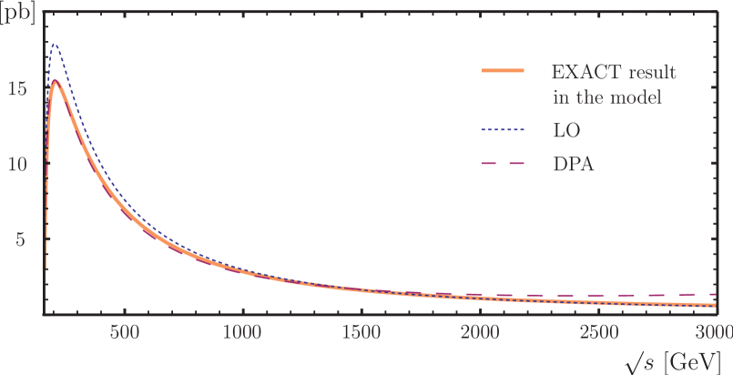
Figure 1: Total cross-section: the exact result in the model, the results in the LO in the MPT (the narrow-width approximation), and in the DPA.

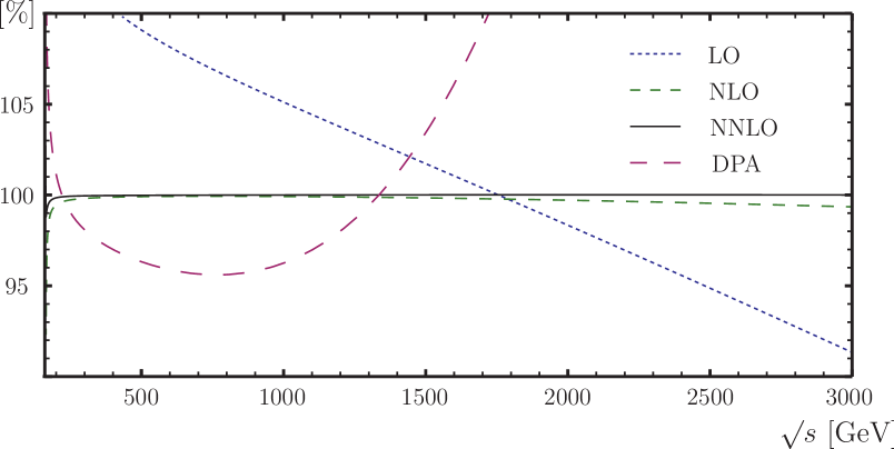
Figure 2: Percentages with respect to “exact” cross-section calculated in the LO, NLO, and in the NNLO approximations in the MPT, and in the DPA.

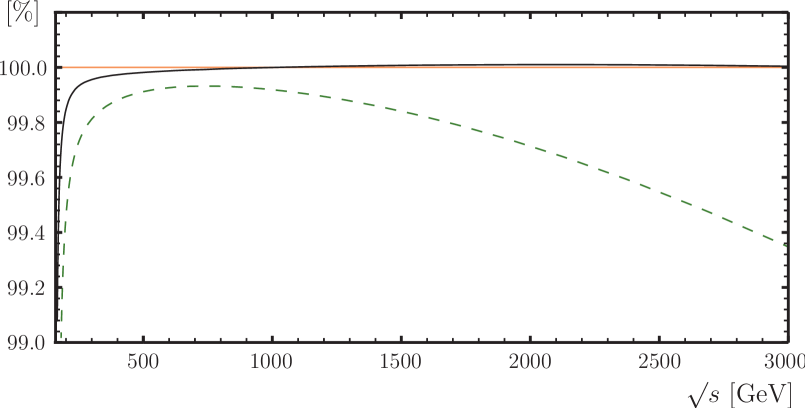
Figure 3: Percentages to the exact cross-section, calculated in the NLO and NNLO approximations in the MPT. The horizontal line at 100.0% means the exact result. The notation for the curves is the same that in Fig. 2.

$\quad\sqrt{s}$ (TeV)	$\quad\;\sigma_{\,\mbox{\tiny EXACT}}\quad$	$\qquad\sigma_{LO}\qquad$	$\qquad\sigma_{NLO}\qquad$	$\quad\sigma_{NNLO}\qquad$
0.2	15.258	17.839	15.175	15.235(2)
	100%	116.92%	99.46%	99.85(1)%
0.5	6.9355	7.5657	6.9294	6.9342(7)
	100%	109.09%	99.91%	99.98(1)%
1	2.8286	2.9733	2.8263	2.8285(3)
	100%	105.12%	99.92%	100.00(1)%
3	0.61023	0.55733	0.60625	0.61026(6)
	100%	91.33%	99.35%	100.00(1)%
5	0.391580	0.24353	0.31047	0.31566(3)
	100%	77.11%	98.31%	99.95(1)%

Table 1: The results of the calculation of the total cross-section in pb and in % with respect to the exact result in the model.

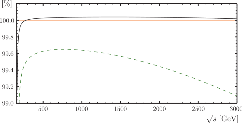
Figure 4: The same as in Fig. 3 but with the other input for widths (see explanation in the text).

The presented outcomes exhibit stable behavior of the NLO approximation and very stable behavior of the NNLO approximation in the energy region beginning with approximately 200 GeV. At the same time, the accuracy of the NNLO approximation in this energy region (more precisely, above 220 GeV) is less than one per-mille. These results remain valid at varying the input-data for the widths $\Gamma^{W}_{2}$ and $\Gamma^{Z}_{2}$, cf. Fig. 3 and Fig. 4. The corresponding shift of the NNLO approximation with the changing of the widths constitutes a few of $10^{-4}$ in relative units. The concurrent shift of the NLO curve exactly follows the shift of the “exact” solution determined by propagator (5), and in relative units constitutes a few of $10^{-3}$. As for the DPA, it has rather non-stable behavior and at high energies it becomes openly bad. In particular, at the energies above 1.5 TeV the DPA becomes much worse even of the narrow width approximation (the LO approximation in the MPT).

In the end of this section it is worth noticing that at the approaching to the threshold of $W$-pair production, the accuracy and stability of MPT rapidly become worse. Actually this behavior was predicted in [10] and was observed at previous calculations [11, 12]. To prevent this difficulty another mode of the MPT near threshold should be applied, which includes Taylor expansion of $\sigma(s)$ not only in powers of $\alpha$, but also in powers of the distance between $s$ and the threshold [10]. A study of the behavior of the MPT in this mode is a task for future investigations.

4 Discussion and conclusions

We have tested applicability of the MPT for description of $W$-pair production in $e^{+}e^{-}$ annihilation. We have found that MPT provides stability of outcomes at the energies beginning with approximately 200 GeV. By means of model calculations we have shown that at the mentioned energies the NNLO approximation in the MPT provides better than one per-mille precision of the description of the total cross-section.

The obtained precision exceeds that observed in the case of the top-quark pair production [12]. The difference is caused by the the lower values of the corrections to the width of $W$-boson as compared to the corrections to the width of the top-quark (and to a lesser degree by the opposite sign of the corrections). Specifically, if we use the corrections to the width of the top-quark in place of those for the $W$-boson (in relative units) in the present calculations, the outcomes for the cross-section in relative units are obtained almost identical to those in the case thoroughly with the top-quark pair production. On the one hand, this confirms the applicability of the MPT in the presence of the large gauge cancellations that occur in the case of the $W$-pair production. On the other hand, this confirms the previous observation that the results of the MPT calculations in relative units depend rather weakly on the particular form of the test function (the amplitude squared without the resonant factors), but depend mainly on the structure of the resonant factors [12]. In total, the above observations mean that the modification of the test function due to turning on the loop corrections, in relative units should not lead to any significant modifications in the cross-section. So, our main results should remain in force in the presence of the loop corrections, in particular, the result about the better than one per-mille precision of the description of the cross-section.

In summary, we conclude that the MPT is really a good candidate for the description of $W$-pair production at the ILC. For a definitive conclusion, of course, a more comprehensive analysis must be made, in particular the analysis of the angular distributions. A study of complete realistic processes, such as CC10, CC11 etc., in the framework of an appropriate model must be made, as well. The mentioned investigations will be carried out elsewhere.

References

- [1] J. Brau et al., arXiv:0712.1950.
- [2] M. Grunewald et al., arXiv:hep-ph/0005309.
- [3] A. Denner, S. Dittmaier, M. Roth and L. H. Wieders, Nucl. Phys. Proc. Suppl. 157, 68 (2006).
- [4] D. Binosi and J. Papavassiliou, Phys. Rev. D66, 111901 (2002).
- [5] A. Denner and S. Dittmaier, Phys. Rev. D54, 4499 (1996).
- [6] S. Dittmaier, in Proc. Int. Europhysics Conf. on High-Energy Physics, Jerusalem, 1997 (Springer, 1997), p. 709.
- [7] A. Denner, S. Dittmaier, M. Roth and L.H. Wieders, Nucl. Phys. B724, 247 (2005).
- [8] F. V. Tkachov, in Proc. 32nd PNPI Winter School on Nuclear and Particle Physics, St. Petersburg, 1998 (St. Petersburg, PNPI, 1999), p. 166.
- [9] M. L. Nekrasov, Eur. Phys. J. C19, 441 (2001).
- [10] M. L.Nekrasov, Int. J. Mod. Phys. A24, 6071 (2009).
- [11] M. L. Nekrasov, Phys. Lett. B545, 119 (2002).
- [12] M. L. Nekrasov, Mod. Phys. Lett. A26, 223 (2011).
- [13] D. Bardin and T. Rieman, Nucl. Phys. B462, 3 (1996).
- [14] A. Denner, Fortschr. Phys. 41, 307 (1993).
- [15] M. L.Nekrasov, Plys. Lett. B531, 225 (2002).
- [16] B. A. Kniehl and A. Sirlin, Phys. Lett. B530, 129 (2002).
- [17] A. Denner, S. Dittmaier, M. Roth and D. Wackeroth, Nucl. Phys. B587, 67 (2000).
- [18] W. Beenakker and W. Hollik, Z. Phys. C40, 141 (1988).
- [19] Particle Data Group Collab. (K. Nakamura et al.), JPG 37, 075021 (2010).
-
[20]
M. L. Nekrasov, in Proc. 13th Int. Workshop ACAT, Jaipur 2010,
http://pos.sissa.it/archive/conferences/093/085/ACAT2010_085.pdf.