Breaks in the Radial Oxygen Abundance and Corotation Radius of Three Spiral Galaxies

Abstract

The correlation between the breaks in the metallicity distribution and the corotation radius of spiral galaxies has been already advocated in the past and is predicted by a chemo-dynamical model of our Galaxy that effectively introduces the role of spiral arms in the star formation rate. In this work we present photometric and spectroscopic observations made with the Gemini Telescope for three of the best candidates of spiral galaxies to have the corotation inside the optical disk: IC0167, NGC1042 and NGC6907. We observed the most intense and well distributed H ii regions of these galaxies, deriving reliable galactocentric distances and Oxygen abundances by applying different statistical methods. From these results we confirm the presence of variations in the gradients of metallicity of these galaxies that are possibly correlated with the corotation resonance.

1 Introduction

The question of what triggers the star formation in the disks of galaxies, and in particular the role of the spiral arms, has been the subject of a long debate. Soon after the theory of spiral arms was proposed by Lin, Yuan & Shu (1969), Roberts (1969) showed that shock waves are produced in the passage of the gas across the spiral gravitational perturbation, and this could trigger star formation. This was not a surprising result, since the arms are obvious to us because they are the areas containing bright stars. Oort (1974), analyzing the gas distribution in M51, suggested that a constant fraction of the gas per passage through the arms is transformed into stars, and consequently that it would be natural to expect the star formation rate to be proportional to $\Omega-\Omega_{p}$. Jensen, Strom & Strom (1976) tested this expression with a sample of nearby galaxies, by plotting a chemical enrichment indicator ([O iii]/H$\beta$) as a function of $\Omega-\Omega_{p}$ , both quantities being measured at a normalized radius, and concluded that the star formation rate is proportional to $\Omega-\Omega_{p}$. However, McCall (1986) argued that the correlation found by Jensen et al. could be the result of independent processes having similar dependence on galactic radius, and presented observations of O abundance gradients in two flocculent galaxies, NGC5055 and NGC7793, which were found to be very similar to those of grand design spirals. As the flocculent galaxies were supposed to be free of spiral arms, the arms could not be the cause of the observed gradients. This argument was later weakened by the fact that a clear spiral structure was found in NGC5055, both in the infrared (Thornley, 1996) and in molecular gas (Kuno et al., 1997). Thornley found infrared spiral structures in several other flocculent galaxies, which is an indication that it is a normal characteristic of these galaxies. Nevertheless, this does not prove that the spiral arms are responsible for the observed gradients. The nature of the flocculent galaxies is not fully understood, and it is not clear if they can be considered (or not) as good examples of galaxies where stochastic self-propagating star formation dominates. As a first step, our effort will be to understand the star formation mechanism in normal spiral galaxies. Zaritsky (1992) investigated the O abundance profile of seven nearby galaxies and found a distinct change in slope for 3 of them. These changes cannot be associated with calibration problems, since precisely the same methods were used in all the cases. Later Zaritsky, Kennicutt Jr. & Huchra (1994) extended the study to a larger number of galaxies, and found for a few of them not only a change of slope, but even possible reversals, with metallicity increasing at large radii (see for instance the profiles of NGC3369). It should be noted that a reversal is easily explained if the star formation rate is considered to be proportional to $|\Omega-\Omega_{p}|$, which is the same expression above but takes into account the cases in which corotation is inside the zone being investigated; a minimum of star formation is expected at $\Omega=\Omega_{p}$. An interesting case is the Milky Way. A simple model of chemical enrichment was proposed by Mishurov et al. (2002) for our Galaxy, in which the star formation rate is proportional to $\Omega-\Omega_{p}$. These authors argue that the minimum (or the plateau) in the gradient of metallicity of our Galaxy, observed using different tracers (eg. Maciel & Quireza 1999, using planetary nebulae and Andrievsky et al. 2004 using Cepheids) is coincident with the corotation radius. The above interpretation for the existence of minima or plateaus in the metallicity gradients is not easy to verify in other galaxies, however, a correlation between radii of minima and/or inflexions in the metallicity distribution and the corotation radius was found by (Scarano & Lépine, 2010) using published data. One of the difficulties to identify the corotation is that this resonance is not necessarily situated in the optical disk. Nevertheless, Canzian (1998) proposed a test to identify galaxies for which the corotation is favorably placed in the optical disk. This test only requires moderately deep imaging and no spectroscopic observations are needed. In this paper we present the study of the radial gradients of metallicity in three of the best candidates identified by the Cazian’s test (IC0167, NGC1042 and NGC6907) to verify if the connection between metallicity breaks and corotation holds for these galaxies. The observations were performed using the Gemini Multi-Object Spectrograph (GMOS), pointed towards 232 H ii regions distributed in these galaxies. Different statistical methods were employed to get O abundances from the observed emission lines. The sample of galaxies and H ii regions are presented in the section 2 of this paper. Observations and data reduction are described in section 3. The photometric and spectroscopic results are presented in section 4. Finally the results are discussed in section 5, where the corotation radii of these galaxies are estimated.

2 Sample Selection

2.1 Galaxies

In order to perform our study we searched in the literature for galaxies for which the corotation is expected to be favorably placed in the optical disk. This was done by selecting three of the best candidates tested by Canzian (1998) (Table 1) according to the following criteria:

1. Galaxies should fail in the conservative version of the Canzian’s test, evaluated by the ratio of the outer to inner extent of the spiral structure. In principle, this guarantees that the corotation is situated in the optical part of the disk (Canzian, 1998);

2. Objects with larger values of the ratio mentioned above were preferred in the selection, since larger ratios means that the corotation radius is deeper into the bright part of the galactic disk (Canzian, 1998);

3. Only galaxies with angular sizes that fit entirely inside the GMOS field (5.5 $\times$ 5.5 arcmin) were chosen. The purpose of this was to cover all the extension of the galaxies with maximum spatial resolution;

4. Each galaxy should have at least 16 H ii regions, since this is the minimum number of H ii regions needed for an ideal sampling to measure the metallicity gradient, according to Dutil & Roy (2001).

5. The three brightest galaxies among those selected with the previous criteria were chosen for observation.

Table 1: Parameters of the selected galaxies. $RA$ and $Dec$ are the equatorial coordinates, $ratio$ is the measured ratio of the outer to inner extent of the spiral structure, $V_{sys}$ is the systemic velocity, $D$ is the Hubble flow distance for $V_{sys}$ ($H_{0}=73km/s/Mpc$), $s$ is the linear scale in the plane of the sky at distance $D$, $a$ and $b$ are respectively the sizes of the major and minor axes, $m$ the total magnitude and $Type$ is the morphological type. (1) Canzian (1998); (2) NED; (3) Scarano Jr et al. (2008)

Parameter	IC0167	NGC1042	NGC6907
RA	1h51m08.5s	2h40m24s	20h25m06.6s
Dec	21∘54′46′′	-8∘26′01′′	-24∘48′34′′
$ratio^{(1)}$	2.41	2.38 / 3.31	2.85
$V_{sys}$ [km/s]	2931(2)	1371(2)	3182(3)
$D$ [Mpc]	41.6	18.6	43.6
$s$ [pc/arcsec]	202	90	211
$a^{(2)}$ [arcmin]	2.9	4.7	3.3
$b^{(2)}$ [arcmin]	1.9	3.6	2.7
$m^{(2)}$	13.6	11.5	11.9
$Type^{(2)}$	SAB(s)c	SAB(rs)cd	SB(s)bc

The fact that the selected galaxies do not have strong bars may simplify the interpretation of the data, since only the secular effect of the spiral arms may be predominant on these galaxies.

2.2 H ii Regions

To perform the spectroscopy we adopted the following procedures to select the H ii regions of each galaxy :

1. Before the GMOS observations we elaborated a list of H ii regions candidates based on the Second Palomar Sky Survey, photometric calibrated using the second release of the USNO CCD Astrograph Catalog (UCAC). The objects were selected according to their flux profile, brightness and geometry;

2. Taking into account that the GMOS supports only one slit per dispersion position and one fixed position angle per observation, we determined instrumental position angles (Table 2) in order to maximize the number of H ii regions candidates to be observed and minimize the number of overlapping spectra in the acquisition process. These position angles were evaluated using the code PAMASKGEM ;

3. After the GMOS pre-imaging using the position angle obtained in (ii) we selected the best candidates H ii regions in each dispersion position. We chose the objects according to their brightness, emission profile (to avoid foreground stars) and colors (as a secondary criterium to exclude foreground stars). Special care was taken to avoid the objects positioned in places where the dispersed spectrum would generate spectral lines away from the GMOS detectors.

3 Gemini observations

The observations were conducted at the Gemini-North telescope in the years 2005 and 2006 using the GMOS Multi-Slit Spectrograph in queue mode. All the observations were executed in better conditions than the minimum required (sky background of $50\%$, cloud cover of $70\%$ and image quality of $70\%$), ensuring full spectrophotometric conditions of the data.

At first the pre-images (Figures 1 to 3) were observed in two filters:(g^′ and r^′). To guarantee a continuous coverage of the GMOS field we applied different dithering patterns to compose a single frame in each filter. Since these images have better spatial resolution than the public data and they are flux calibrated, we used them to refine the H ii region selection, as described before. The combination of these results with the morphological data allowed us to design the metallic masks where the slits were placed for the spectroscopic observation. Inclinations and position angles were estimated from the isophotes of the final images of each galaxy. Table 2 summarizes the information for these observations.

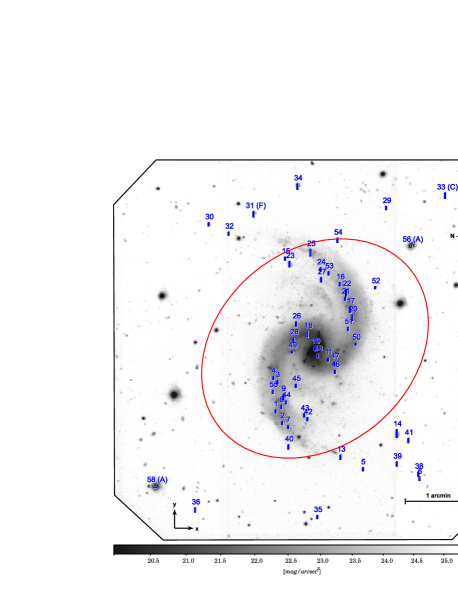
Figure 1: Slits superimposed to the r^′image of the galaxy IC0167. Only the slits used in the 2006 observations are presented. ”A” are the stars used for alignment, ”F” are reference stars for flux calibration and ”C” is a slit used for sky sampling. The sky orientation is given by the N-E compass and the spectral dispersion follows the x direction of the x-y compass. The ellipse represents the projection of a circle in the sky plane considering the same inclination and position angles obtained from the spiral arms.

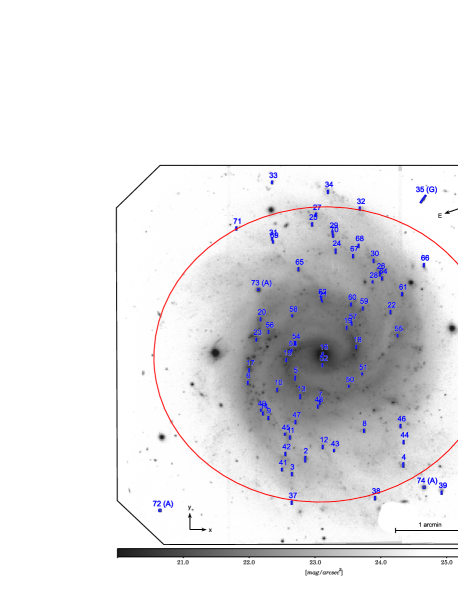
Figure 2: Slits and elliptical fitting superimposed to the r^′image of the galaxy NGC1042. The same definitions used in the previous picture are used here. Slits with a ”G” sample galaxies in the field.

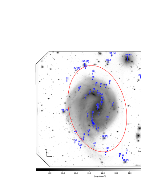
Figure 3: Slits and elliptical fitting superimposed to the r^′image of the galaxy NGC6907. The definitions here follows those used in the two previous pictures.

Table 2: Observational parameters for the pre-imaging process of the galaxies IC0167, NGC1042 and NGC6907 in each one of the filters g^′and r^′. $UT$ is the universal time when the observation started, $t_{exp}$ is the exposition time, $n_{exp}$ is the number of exposures for the dithering pattern, $PA_{instr}$ is the instrumental position angle and $OIWFS$ is the USNO UCAC2 Catalog index of the star used as the on-instrument wavefront sensor. All the observations were conducted at 2$\times$2 binned mode.

	IC0167		NGC1042		NGC6907
Parameter	g′	r′	g′	r′	g′	r′
UT	16/8/2005	16/8/2005	6/9/2005	6/9/2005	1/8/2005	1/8/2005
	14:31:36	14:38:57	12:58:18	13:09:54	08:03:12	08:09:04
texp [s]	150	120	240	90	360	120
nexp	5	4	8	3	12	4
PAinstr [∘]	265	265	19	19	243	243
Airmass	1.001	1.001	1.179	1.163	1.691	1.66
Seeing [′′]	0.99	0.74	0.78	0.68	0.63	0.63
OIWFS Star	39427277	39427277	28845687	28845687	21894023	21894023

After the mask design the spectroscopic observations were carried out doing individual exposures from 960 to 1200 seconds using the B600$\_$G5303 grism centred at two different wavelengths to cover the spectral range from 3500 Å to 7100 Å. With this coverage and considering the systemic velocity of the galaxies the main spectral lines required for metallicity evaluation could be observed. No spectral dithering was used to cover the GMOS gaps in the final spectra. So, taking this into account, the choice of H ii regions only considered the slits in positions that would not generate important spectral lines on the detector gaps. A CuAr arc lamp and a flat-field frame were observed in the sequence of the spectroscopic acquisition, while the telescope was still following the source, to guarantee the quality of the calibrations by avoiding any effect caused by instrumental flexures. The same OIWFS stars used in the pre-image process were used for the spectroscopy. Information about the spectroscopic observations can be found in Table 3 and the details of the slits in Tables 5 to 11.

Table 3: Observational details for the GMOS spectroscopy of the galaxies IC0167, NGC1042 and NGC6907 in 2005 and 2006. $UT$ is the universal time when the observation started, $t_{exp}$ is the exposition time $\lambda_{c}$ is the central wavelength of the dispersed light, $Band$ is the spectral range coverage, $n_{slit}$ is the total number of slits. The instrumental position angle was the same used for the pre-images and an 1 arcsec slit width was adopted in all observations. In 2005 the height of the slits were fixed in 5 arcsec but in 2006 their sizes changed to improve the number of observed H ii regions. The spectral resolution achieved is around 1700.

	IC0167		NGC1042		NGC6907
Parameter	2005	2006	2005	2006	2005	2006
UT	6/9/2005	23/8/2006	5/11/2005	24/8/2006	2/9/2005	22/8/2006
	11:40:27	14:41:54	10:34:08	14:56:00	06:04:33	09:30:27
texp [s]	960	1200	1200	1200	960	1200
$\lambda_{c}$ [Å]	5000	5900	5000	5850	5000	5950
Band [Å]	3500-6300	4400-7200	3500-6300	4350-7150	3500-6300	4450-7250
nslits	34	52	35	68	36	57
Airmass	1.06	1.018	1.154	1.137	1.618	1.453
Calib. Star	G191B2B	Feige34	G191B2B	Feige34	G191B2B	Feige34

4 Data Reduction and Analysis

Standard procedures for reduction of GMOS imaging and spectroscopy were followed. In both cases the general Gemini Data Reduction Software was used. The details about this can be found in Scarano et al. (2008) for the specific case of NGC6907. The same procedures were carried out for IC0167 and NGC1042.

For each filter the multiple dithered frames were mosaiced and co-added. This procedure improved the signal-to-noise ratio of the final images removing both cosmic rays and the gaps between the GMOS detectors. Since the spectroscopic data corresponds to a single frame, the cosmic rays events were synthetically removed using the task GSCRREJ (more details about in the task documentation). In these cases the GMOS gaps were linearly interpolated. Wavelength calibration was performed using the individual arc lamps observed just after the spectroscopic acquisition. For each individual slit the spatial distribution was used to improve the spectral calibration. The sky lines and the continuum were removed from the main source using the contiguous data in the spatial direction of each slit.

4.1 Photometry

The photometric calibration in filters g^′and r^′was performed using the photometric standard stars supplied by the Gemini baseline, listed in Table 3. Usual procedures applying DAOPHOT IRAF tasks enabled us to recover the zero point magnitudes, taking into account the effects of the atmospheric extinction and the corrections for the galactic extinction by Schlegel, Finkbeiner & Davis (1998) and Amôres & Lépine (2005). Assuming the limit of detection of the galaxies as the $3\sigma$ limit of dispersion of the local sky level, elliptical fittings were performed for the estimation of the inclination and position angle of the galaxies. However, as next explained, we did not use the parameters obtained in this way to derive the distances of H ii regions to the galactic centres.

After the conversion of the g^′and r^′images to the B and V bands, using the expressions by Fukugita et al. (1996) and Hook et al. (2004), we obtained surface brightness profiles similar to those presented by Canzian (1998). However, the inclination and position angles that we derive do not match with previous works like Canzian (1998) and de Vaucouleurs et al. (1992), even when we apply corrections such as masking the data from the contribution of stellar fields, the interarm regions and the disturbed parts of the galaxies. But this is only part of reasons for giving preference to other methods to determine inclinations and position angles. The method of fitting ellipses to the isophotes, although commonly adopted, is based on the questionable hypothesis that the spiral galaxies isophotes are approximately circular when seen face-on. This is particularly incorrect in the case of two-armed spirals with large pitch angles, for which the light distribution is naturally elongated in the direction of the extremities of the arms, the so-called Stock s effect (Stock, 1955). The other methods available are the kinematic method, which consists in finding the axes of the spider diagrams or iso-velocity contours in H i maps, and spiral-arm fitting, which is based on the assumption that large parts of the arms are logarithmic spirals. Our group performed H i observations with the GMRT (Giant Meterwave Radio Telescope) of the three galaxies, but for the moment, the results are published only for NGC6907 (Scarano et al., 2008), where a detailed discussion of its inclination can be found. While the other results are not published, the contradiction between photometric and kinematic results can be seen from the orientation of the velocity fields presented for NGC1042 by Kornreich et al. (2000) and for IC0167 by van Moorsel (1988). On the other hand, Ma (2001) proposed a method that uses the spiral arms fitting, and applied it to several galaxies, including IC0167 and NGC6907. Applying his method to both arms of NGC1042 we got consistent values for inclination at a given position angle. We found that the kinematic and spiral arm fitting methods give similar results, which differ from the isophotal ellipse fitting. We conclude that the spiral arm fitting method is reliable in the present cases, and adopted its results in the following analysis (Table 4).

Table 4: Photometric and morphologic results for IC0167, NGC1042 and NGC6907 using GMOS. The values with a ”*” are from Ma (2001). For the photometry, the symbol $m$ is used for total magnitude, $\Sigma$ for surface brightness, measured in mag/arcsec^-2, $M$ is the absolute magnitude and L the luminosity, in $L_{\odot}$. For the morphology, $i$ and $\phi$ are the inclination and the position angles ($isoph$ index for isophotal elliptical fitting and $spir$ index for the results derived from the spiral arms), $RA_{0}$ and $Dec_{0}$ are the equatorial coordinates of the spiral arms centre (which coincide with HI velocity center as mentioned in the text), $\alpha$ is the pitch angle of the spiral arms, all in degrees and finally $a$ and $b$ are major and minor semi-axis of the ellipse, in arcmin.

Parameter	IC0167	NGC1042	NGC6907
$m_{0,g}$	31.49 $\pm$ 0,15	31.47 $\pm$ 0,16	31.4 $\pm$ 0,15
$m_{0,r}$	31.79 $\pm$ 0,17	31.77 $\pm$ 0,21	31.72 $\pm$ 0,14
$m_{g}$	11.11 $\pm$ 0,29	9.84 $\pm$ 0,20	10.45 $\pm$ 0,04
$m_{r}$	10.26 $\pm$ 0,27	9.16 $\pm$ 0,19	8.90 $\pm$ 0,03
$\Sigma_{g}$]	21.95 $\pm$ 0,57	21.80 $\pm$ 0,44	21.3 $\pm$ 0,08
$\Sigma_{r}$	21.17 $\pm$ 0,56	20.95 $\pm$ 0,44	19.7 $\pm$ 0,07
$M_{B}$	-21.07 $\pm$ 0.47	-20.63 $\pm$ 0.41	-21.70 $\pm$ 0.35
$L_{B}$[1010	3.9 $\pm$ 1.7	2.6 $\pm$ 1.0	7.0 $\pm$ 2.2
$\Sigma_{lim}^{g}$	26.26 $\pm$ 0,57	26.33 $\pm$ 0,44	25.74 $\pm$ 0,08
$\Sigma_{lim}^{r}$	25.44 $\pm$ 0,56	25.4 $\pm$ 0,44	24.86 $\pm$ 0,07
$RA_{0}$	27.785629	40.099802	306.277600
$Dec_{0}$	21.912776	-8.433441	-24.809200
$a_{isoph}$	1.82 $\pm$ 0.04	2.49 $\pm$ 0.15	1.47 $\pm$ 0.02
$b_{isoph}$	1.15 $\pm$ 0.03	2.01 $\pm$ 0.10	1.29 $\pm$ 0.02
$i_{isoph}$	51.5 $\pm$ 3.0	36.3 $\pm$ 3.1	29.1 $\pm$ 3.0
$\phi_{isoph}$	73.1 $\pm$ 15.8	12.5 $\pm$ 8.5	254.1 $\pm$ 3.3
$i_{spir}$	38.0 $\pm$ 3.0*	29.0 $\pm$ 2.9	49.5 $\pm$ 3.0*
$\phi_{spir}$	134.0 $\pm$ 3.0*	277.4 $\pm$ 5.1	239.9 $\pm$ 3.0*
$\alpha$	26.6 $\pm$ 1.9*	13.3 $\pm$ 2.5	23.5 $\pm$ 5.0*

The radial surface brightness profiles (Figure 4) were obtained performing the integration of the flux on elliptical rings with the same thickness of the seeing and following the parameters of projection imposed by the spiral arms (Table 4). Since there is an interaction between NGC6907 and NGC6908, confirmed by Scarano et al. (2008), a detailed discussion of the photometry of NGC6907 can be found in that paper.

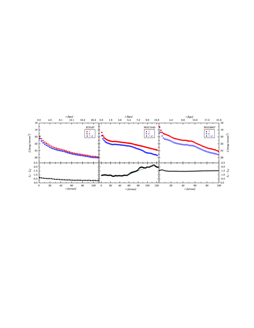
Figure 4: g^′ and r^′ radial surface brightness (top) and color profiles (bottom). Remark that in both the order of the filters and the scale are not conventional.

4.2 Spectroscopy

With the spectrophotometric calibration stars supplied by the Gemini baseline (Table 3) we determined the sensitivity function and then each spectrum could be flux calibrated.

Considering that all spectral lines have their wavelength systematically changed by the systemic velocity of the galaxies, and locally changed by the projection of the rotation curves on the line of sight, we used the IRAF package RVSAO (Kurtz & Mink, 1998) to determine radial velocities and identify the typical spectral lines observed in H ii regions by cross-correlating a template spectrum to the observed spectra. The measured velocities and their errors are given in Tables 5 to 13. We then integrated the flux of lines, performing the following steps:

1. According to the galactic coordinates of each slit the related spectrum was corrected by the galactic extinction using the reddening calculated by the code EXTIN written by Amôres & Lépine (2005) and an IDL adaptation of the code FMCURVE by Fitzpatrick (1999) called FM_UNRED;

2. Using the expected ratios between Balmer lines (Osterbrock, 1989) we measured the flux of the hydrogen lines and estimated the intrinsic reddenings of each spectrum employing the relations written by Fitzpatrick (1999), which were introduced in the FM_UNRED code to correct the spectra by the intrinsic reddening;

3. Taking into account the wavelengths determined for all recognized spectral lines we performed the integration of the flux of them, by considering the robust mean of the area under the line profile evaluated by the following procedures: (a) Gaussian fitting; (b) Lorentzian fitting; (c) numerical integration; (d) double gaussian fitting;

4. With the fluxes and uncertainties evaluated in the previous step, the metallicities were calculated using statistical methods to determine O abundances. The methods applied were the R23 method of Pagel et al. (1979) with the considerations of McGaugh (1994), the [O iii]/[N ii] method of Pettini & Pagel (2004) and Stasińska (2006), the [N ii]/$H\alpha$ method of Pettini & Pagel (2004), the [Ar iii]/[O iii] method of Stasińska (2006) and the p-method of Pilyugin (2000) and Pilyugin (2001).

We next present more details on the steps described above. Since the interstellar medium affects differentially the flux of the spectral lines, the correction of the spectra by the extinction is fundamental to estimate metallicities. To do this we need to distinguish two contributions: one from our Galaxy (the galactic extinction) and the other internal to the observed galaxies (the intrinsic extinction). A model for the galactic extinction is well established by Amôres & Lépine (2005) and we applied their model to correct all spectra by the galactic flux losses. Supposing that the remaining differences in the ratio of the Balmer lines are a consequence of the intrinsic extinction in the observed galaxies and that their extinction laws are similar to the Galaxy extinction law, each spectrum was corrected again by determining the reddening from the Balmer line ratios and using it in the Fitzpatrick (1999) code. In spite of the evidences from the Megellanic Clouds that extragalactic reddening laws may not be rigorously the same one we observe for our Galaxy, the comparison between the results of Gordon et al. (2003) for the Megellanic Clouds with the Fitzpatrick (1999) extinction law reveals that at least in the optical part of the spectrum, where the O abundances are calculated, this hypothesis may be assumed. This was already done in the past (eg. Misselt, Clayton & Gordon 1999, working with 11 spiral galaxies) and it has the advantage of correcting the rising of the extinction as a function of the galactic inclination (Unterborn & Ryden, 2008). The Tables 15 to 20 contain the values we got for intrinsic extinctions. Typical spectra of each one of the observed galaxies corrected for both extinctions can be seen in Figure 5. Ultimately the results would be the same if we ignored the extinction components and only the total reddening correction using the Balmer lines were considered.

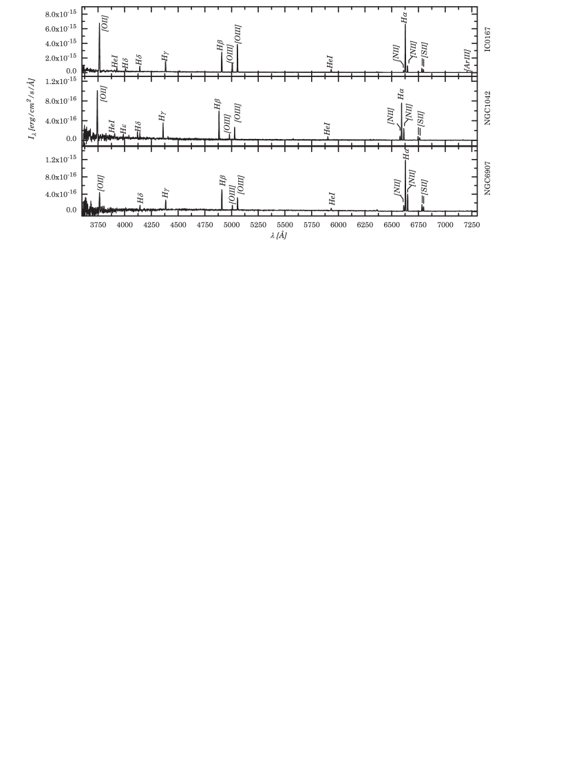
Figure 5: Typical spectra of the galaxies IC0167 (top), associated to slit 18 (2006), NGC1042 (middle) from slit 21 (2006) and NGC6907 (bottom) related to the slit 29 (2006). Each spectrum combines the data from 2005 and 2006 observations

The option of measuring the fluxes using four procedures was a way to automatically register the differences between the spectral lines profiles in each spectrum. The robust mean of these fluxes is equivalent to the mean of the two best fitting procedures, since in this method the ”discrepant” values are discarded. In our case the best fitting procedures were the Gaussian fits and the numerical integration. But the mean between these two procedures is exactly the method adopted by Zaritsky et al. (1994) to measure the line fluxes of his sample. The advantage of our method is that it allowed us to automatically compare and identify profiles affected by cosmic rays remnants, bad sky line subtraction, lines with unusual profiles and blended lines. We adopted uncertainties associated to the robust standard deviation of the measured fluxes in such way that larger uncertainties are a consequence of less defined profiles and lines with lower signal-to-noise ratio. These results were verified by computing the Poissonian errors directly from the number of photon counts in the lines and the results are in perfect agreement with our method. Typically these values are smaller than 10% but considering differential effects each spectral line has its own typical value (see Tables 21 to 23).

One of these effects is the differential atmospheric refraction. Depending on the airmass, seeing, slit width and slit orientation relative to the parallactic angle the observations may be more or less affected by this kind of refraction. According to our specifications, observations were conducted in seeing conditions better than 0.7”, while the standard slit width of 1” was adopted for all objects. Since for the MOS observations the position angles of the slits are fixed and our observations were carried out in queue mode, we were not able to tune the slits position angles to the parallactic angles. Nevertheless, except for the observation of NGC6907 in 2005 all observations were performed with position angles of the slit differing less the 15 degrees from the parallactic angle. Unfortunately NGC6907 is always observed in large airmasses at Mauna Kea, and this affected both observations of this galaxy.

Considering only the differential wavelength effect of the airmass on the atmospheric refraction, we verified that the [O ii] spectral line was severely affected in the observations of NGC6907 in 2005. For these observations the center of the H ii regions were deviated at least 0.5” outside the slit width; this means that the observed [O ii] lines come predominantly from the borders of the H ii regions. Moreover, the slit orientation relative to the parallactic angle in 2005 was almost 80 degrees, which means that more than 85% of the [O ii] emission line was not detected.

Fortunately the situation was different for all the other observations. Taking into account the redshifts of the galaxies, the worst airmasses and the largest deviation of the slit orientation relative to the parallactic angle, the [O ii] flux losses represents less than 5% of the total [O ii] emission. This is the particular situation of NGC1042 observed in 2005. Since IC0167 was observed almost in the parallactic angle and airmass 1, there was no effect of atmospheric refraction. Furthermore, for the 2006 observations we only used spectral lines above $H\gamma$, for which the atmospheric refraction effects are negligible given our slit widths.

Another thing that must be considered is the underlying Balmer absorption. The corrections are usually done by measuring the equivalent widths of the Balmer lines and applying the procedures by McCall, Rybski & Shields (1985) and Oey & Kennicutt (1993). According to Zaritsky et al. (1994) such correction amounts to less than 10% for 75% of the regions he studied. Given that for most of the spectra we observed there is no evident absorption profiles in $H\alpha$, $H\beta$ or $H\gamma$ (used to correct the spectra for reddening and as references for abundance determinations) we opted to eliminate from our analysis the objects for which the $1\sigma$ level of the background affected by the Balmer absorption represents more than 10% of the peak emission. It represents less than 20% of the observed regions in 2005 and about of 10% of our sample observed in 2006. Given the proportions presented by Zaritsky we believe that the worst effect of the Balmer absorption was eliminated from our sample.

5 Results and Discussion

The first step to determine O gradients is to evaluate the O abundances and the radial distances inside de galactic planes. Following the procedures mentioned in the previous section, the flux of each spectral line needed to calculate the O abundances using the statistical methods was determined and registered in Tables 21 to 23. Some individual lines may present underestimated uncertainties, nevertheless the errors on the abundances, derived by propagating the flux uncertainties of all spectral lines involved, are around 0.2 dex, coherent with those mentioned in the literature (see Pilyugin, Vílchez & Contini 2004 and references therein). Using the inclinations, position angles and the galactic centre coordinates determined using the spiral arms (Table 4), the distances to the H ii regions sampled by the slits (Tables 5 to 13) were calculated with the expressions given by Scarano et al. (2008). These expressions introduce important corrections to the more traditional ones (eg. Begeman 1987). For the galaxies studied here these corrections reach up 20% of the distances calculated with the previous procedures. Since the deviations on the corotation radius range between 2 and 3 kpc the corrections are needed to avoid a too large smoothing of the radial distribution of metallicity.

For each galaxy the systemic velocities were obtained by taking into account the radial velocities measured from all the observed spectra and calculating the weighted mean of their distribution. Such procedure is a raw measurement, which assumes that the receding and the approaching sides of the galaxies were evenly sampled. In spite of that, the results are in agreement with those found in the literature (Table 1). A few objects were found to be background galaxies or isolated objects instead of H ii regions belonging to the galaxies we study here; they were eliminated from the sample based on their velocities. The velocity distribution of the H ii regions of each galaxy is approximately Gaussian, and we discarded the objects more than 3 HWHM (half width at half maximum) off from the center of the distribution.

Remembering that each observational run was optimized for a given spectral range we present in Figure 6 the best O abundances calculated for each galaxy using the spectral lines available in that run. Since in 2005 observations the [O ii] line was present and $H\alpha$ was not, we applied the R23 based-methods to determine O abundances, represented here by the p-method (Pilyugin 2000 and Pilyugin 2001). On the other hand, for the 2006 observations, the [O ii] line was out of the range and only the methods that use the $H\alpha$ and $H\beta$ lines could be applied, in particular [O iii]/[N ii] methods, represented here by the Stasińska (2006) method. The advantage of the p-method is that it can provide O abundances with precision comparable with the direct methods, based on the temperature sensitive line ratios, however it is double-valued at low abundances. Note that the 2005 observations could only be corrected for extinction by measuring the $H\beta$ to $H\gamma$ ratio, since $H\alpha$ was not available. This provides a poorer correction than the $H\alpha$ to $H\beta$ ratio. In contrast to the p-method, the [O iii]/[N ii] Stasińska’s method is single valued, with the advantage that it is relatively independent of the reddening (Stasińska, 2006).

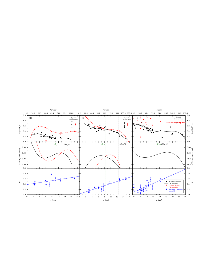
Figure 6: Radial O abundance, fitted by a 4th order polynomial (top), the derivative of the fitted curve (middle) and the distribution of the excitation parameter P (bottom). The stars represent the results of the 2005 observations, analyzed with the Pilyugin’s method, and the circles symbolize the observations of 2006, analyzed using the Stasińska’s method. For each case the opened symbols indicated the typical uncertainties. The vertical lines labeled with a $R_{CR}$ indicated the estimated position of the corotation radius and those labeled with a $D0_{25}/2$ mark the position of the isophotal radius where the surface brightness falls to $25mag/arcsec^{2}$. The panels are: (a) IC0167 (left), (b) NGC1042 (center), (c) NGC6907 (right). In this last case the differential refraction leads to a so huge scatter when the Pilyugin technique was applied, so it was not used in the further interpretations.

A constant gradient has been the most commonly adopted law in the study of metallicity of galaxies. This is a first approximation, not a choice dictated by theory. For instance, most chemical abundance models adopt star formation rates proportional to some power of the gas density, and most often the gas density presents a peak at several kpc from the center. The stellar density in the disk of our Galaxy is better described by Kormendy’s function than by an exponential law (see Lépine et al. 2000). We make here the choice of fitting the data with 4th order polynomials. This does not correspond to a theoretical model of galactic structure; the polynomial fitting is only adopted as a smoothing method instead other methods like splines or Gaussian filtering, which could be used alternatively. One advantage of the polynomial method is that it gives the position of minima and inflections in an easy way. The choice of the 4th order corresponds to the amount of details that we are willing to reveal. For instance in our Galaxy, the observations of Cepheids (Andrievsky et al. 2004) show that there is a strong metallicity gradient in the inner regions, followed by a plateau, followed again by a another strong gradient. Such a behavior, that we expect to observe in other galaxies as well, can be approximated by a 4th order polynomial.

It is known that the different statistical methods used to calculate the O abundances can result in different values for a same observation, and they can produce different dispersion of the data with respect to an average abundance profile, and also small differences in the gradients, specially for those methods which do not depend directly on the O ionic abundances. In our observations the largest differences occurred between the p-method and all the other mentioned methods. This seems to be a consequence of the strong dependence of the p-method on the [O ii] emission line, which is observed at the limit of the instrumental sensitivity and it is strongly affected by the reddening and the parallactic angle misalignments.

For IC0167 most of the methods applied here point towards the existence of a very smooth minimum in the O abundance profile, which is shallower than the one of our Galaxy, according to Mishurov, Lépine & Acharova (2002). In particular, the distribution produced by the p-method is more dispersed than the results for the [O iii]/[N ii] method, however the minima in the O abundance obtained with the two methods almost coincide. The median of the minima and inflections found using all the methods applied to this galaxy is $14.7\pm 2.6$ kpc. Obviously it is necessary to be cautious in the interpretation of the fitted curves. The trend could be fitted by a straight line and the evidence for an inflection is not very strong in this case.

On the other hand, for NGC1042, the abundance dispersion is less pronounced and a plateau is present in the O abundance profiles of this galaxy obtained by means of the [O iii]/[N ii] p and R23-based methods. This plateau could possibly be interpreted as being a consequence of the corotation as well, but in this case the minimum is too shallow to contrast with the dispersion of the data. The dispersion resulting from the two calibrations of [N ii]/$H\alpha$ method of Pettini & Pagel (2004) and the [Ar iii]/[O iii] is so high that no consistent information can be extracted. Since the point of inflection is a point which is close to being a minimum (see the lower curves in Figure 6 for NGC1042), we could speculate that it is also an indicator of the corotation. The median of the inflexions of the abundance curves for NGC1042 is $8.2\pm 2.8$ kpc. Interestingly, at this same position a small bump also can be observed in the color distribution of this galaxy (Figure 4). This might be connected with corotation as well, since a gap in the density distribution of young stars can be expected at corotation, as it happens in our Galaxy (Amôres, Lépine & Mishurov, 2009). The lack of young stars would make this region slightly redder than its neighborhood.

Finally, a bimodal behavior in the radial distribution of O is found for NGC6907 using the [O iii]/[N ii] method. Since the Argonium line is not detected along all the galaxy, the spatial distribution of metallicity derived from this element is inconclusive. The same happens using the [N ii]/$H\alpha$ method, which results in O abundances with large dispersion at radii beyond 15 kpc. Unfortunately the observations of 2005 were not performed near the parallactic angle and for this reason the measurements of the [O ii] lines are not reliable, causing a huge dispersion of the O abundances derived by the R23 and p-method. Since the nucleosynthetic origin of the nitrogen may shift from secondary to primary in low abundances H ii regions we need to be more cautious to interpret the inflexions in the NGC6907 abundance distribution. The median of the radii of the minima found using the other statistical methods is $21.1\pm 3.7$ kpc. Scarano et al. (2008) have shown that for this galaxy there is a minimum in the H i gas distribution between 20 and 30 kpc, which can be related with the same effect of the corotation found in our galaxy by Amôres et al. (2009).

The interpretation of the gradient of metallicity for NGC6907 may seem dangerous, since this galaxy is interacting with NGC6908 as discussed by Scarano et al. (2008). However the same authors have shown that the influence of this galaxy on the NGC6907 gas distribution is restricted to about 20^∘around NGC6908, in azimuthal angles measured in NGC6907 galactic plane. Except for the spectra sampled by the slit 25 in the 2006 run, all the other slits associated to radii greater than 15 kpc are situated on the side opposite to the one where the interaction with NGC6908 takes place. Similarly to what happens with the rotation curve, which is not perturbed on that side (Scarano et al., 2008), we expect that the metallicities of the H ii regions presented here are not affected by the interaction.

Are the polynomial fits really better than the traditional straight line fits? It should be remembered that we do not consider that the 4th order polynomials are models, but only a technique used for locating changes in the slope. If the changes in slopes and plateaux are real then, in principle, the polynomial fit should be better. But of course, a 4th order polynomial always produces a better fit than straight line, as long as the rms deviations of the data with respect to the fitted curve are taken as the measure of the quality of the fit. To determine if a polynomial fit is effectively a meaningful choice, one must compare the chi-square divided by the degree of freedom $N-k-1$, where $N$ is the number of data points and $k$ the order of the polynomial (see the discussion in Chapter 15 of Numerical Recipes ((Press et al., 1992)). We performed these tests, and the results can be summarized as follows: after correction for the degree of freedom, the adjustments by 4th order polynomials are slightly better (the chi-square obtained with straight lines are larger by a factor which ranges from 2 to only a few percent). In other words the straight lines are not the best choice, but they cannot be excluded on statistical grounds. Testing different orders of polynomials from 2 to 6, in all cases the 4th order is slightly better than all the others except for NGC1042 for which the 3rd order polynomial gives a slightly smaller (3%) normalized chi-square. This last result still suggests that an inflection point is present.

Pilyugin (2003) argued that the bends in the slopes of radial abundance gradients in the disks of spiral galaxies is a consequence of a systematic error involving the excitation parameter P, which would produce realistic O abundance in high-excitation H ii regions, but would overestimate this abundance in low excitation H ii regions. For a measured value of R23, there are two possible solutions for the O abundance. For instance, according to Pilyugin, the positive slope of the observed O abundance by Roy & Walsh (1997) in the external regions of the galaxy NGC1365 would be changed into a negative slope, and the break would disappear, if one used the lower branch of the graph of O abundance versus R23 for these regions. The question, then, is when one should move from one branch to the other, to use correctly the method. According to Pilyugin’s calibrations (Pilyugin, 2003), the upper branch corresponds to $12+log(O/H)>8.15$. As can be seen in Figure 6, the slope breaks are situated above this abundance threshold for two of the galaxies studied here (NGC1042 and NGC6907), so they cannot be explained by a change of the O abundance versus R23 law. One argument given by Pilyugin to justify the existence of bends above the previous limit is that the less the value of the excitation parameter P the more the oxygen abundance obtained with the R23-method is overestimated (Pilyugin, 2003). However, even with an increasing behavior of the excitation parameter at radii larger than the radius identified as the corotation radius for NGC1042, the overall decreasing behavior of the radial metallicity distribution is not flattened by the almost linear radial increase of the excitation parameter P. It only presents a small step in the region where the corotation seems to occur. Another important point to be considered is that, in contrast to the R23 or the p-method the [O iii]/[N ii] method is single-valued and for the galaxies observed here we verified minima and inflexions independently of the R23-based methods. One might worry that [O iii]/[N ii] could depend upon a second parameter near co-rotation, and the behavior of the excitation parameter might even suggest a correlation with the corotation radius, but such an hypothesis would have to be investigated in a large sample of galaxies, and for the moment, it is not supported by any theoretical prediction.

This is not the first time that breaks in the radial distribution of metallicity are associated to the corotation radius. The break observed by Roy & Walsh in NGC1365 is real, as it has been observed using different calibrations and not only R23, and in addition, the break appears at $12+log(O/H)=8.7$, well in the upper branch defined by Pilyugin. Roy & Walsh (1997) verified that the position of the metallicity break that they found in NGC1365 is beyond the corotation radius found by Jorsater & van Moorsel (1995). Remembering that the Mishurov’s model for our Galaxy, as well as the more recent one by Acharova et al. (2010), claims that the chemical evolution of a galaxy is proportional not only to the difference between the spiral pattern speed and the angular velocity of the rotation curve, but also depends on the surface density of the gas, so a small displacement of the metallicity break with respect to the corotation radius can be understood. In NGC1365, there is an intense star formation activity in the bar, at a radius slightly smaller than the corotation radius, in a region where the gas density is higher than average. Slightly beyond the corotation radius, there is steep decline in the gas density (Jorsater & van Moorsel, 1995). The presence of a strong gas density gradient across the corotation radius displaces the metallicity minimum simply because the star-formation rate depends strongly on that density (see the details of Mishurov’s model).

6 Conclusions

The analysis of the gradient of metallicity of our Galaxy by Mishurov et al. (2002) leads us to infer that in other galaxies as well, we should expect that minima or inflexions in the radial gradient of metallicity could be correlated with the corotation radius. One indication that the same process also happens to other galaxies was obtained with the correlation found between the minima and inflexions in the metallicity distribution, using published data and the procedures presented here, and the corotation radius from different references available from the literature (Scarano & Lépine, 2010). In order to test this prediction we performed photometric and spectroscopic observations of three of the best candidates pointed by Canzian (1998) to have the corotation inside the optical disk, IC0167, NGC1042 and NGC6907.

Using images obtained with the Gemini Telescope, we conducted a careful procedure to select H ii regions to be observed with the GMOS. To avoid the problems with the isophotal elliptical fittings found for these galaxies, caused by their prominent spiral structure, we adopted the procedure recommended by Ma (2001) to determine the inclination and the position angles. This allowed us to calculate more reliable distances in the galactic plane, since for these galaxies the spiral arms provide results which are coherent with the velocity fields found by Scarano et al. (2008), Kornreich et al. (2000) and van Moorsel (1988).

The first spectroscopic run was optimized for the blue part of the spectra, for which the R23-based methods could be applied, in particular the p-method, while the second run was optimized to the red part of the spectra, and the [N ii]-based methods could be employed. The number of observed and effectively used spectra in this project changed according to the run but with the observations of 2006 we overcome the minimum data sample advocated by Dutil & Roy (2001) for an ideal measurement of the metallicity gradient. All data were corrected for galactic and intrinsic extinctions and the data affected by the underlying Balmer absorption was removed from the analysis. By fitting polynomials of different orders to the radial metallicity distribution of the three galaxies, we found that the 4th order polynomials produces better fits than first order (straight lines) in all the cases, even when correcting the chi-square for the larger number of degrees of freedom of the 4th order polynomial. The radii of the minima or points of inflection derived from the statistical methods of determining the abundances adopted here are in relatively good agreement. We recognize, however, that since the gradients and their variations have small amplitudes, we cannot totally exclude the possibility of an interpretation of the data in terms of straight lines. Furthermore, since the Canzian s method only gives us the best candidates of galaxies that have the corotation radii inside the optical disk, it is not possible for the moment to clearly associate the changes in gradient slopes with corotation. If we assume that the minima and inflections are situated at the corotation radius, for IC0167, NGC1042 and NGC6907, the corotation is at $14.7\pm 2.6$, $8.2\pm 2.8$ and $21.1\pm 3.7$ kpc respectively. Further studies have to be conducted to verify if these estimates of corotation radius are confirmed by other methods.

7 Acknowledgements

This work is based on observations obtained at the Gemini Observatory, which is operated by the Association of Universities for Research in Astronomy, Inc., under a cooperative agreement with the NSF on behalf of the Gemini partnership: the National Science Foundation (United States), the Science and Technology Facilities Council (United Kingdom), the National Research Council (Canada), CONICYT (Chile), the Australian Research Council (Australia), Ministério da Ciência e Tecnologia (Brazil) and Ministerio de Ciencia, Tecnolog a e Innovaciǿn Productiva (Argentina) The work was supported by the Sao Paulo State Agency FAPESP through the grant 09/05181-8. This research has been benefited by the NASA’s Astrophysics Data System (ADS) and Extra-galactic Database (NED) services. Their open software used in this research is greatly acknowledged. The Gemini programme ID for the data used in this paper is the GN-2005B-Q-39 and GN-2006B-Q-89 (PI: S. Scarano Jr). We would like to thank the referee Marshall McCall for his careful and critical reading of the earlier versions of this paper and for his numerous valuable and substantial suggestions for improvements of the paper.

Appendix A Positions, Distances and Velocities Associated to the Slits

In this appendix we compile the information about the sky coordinates of the slits and its height (RA (J2000), Dec (J2000), $\Delta$y), the correspondent face-on polar coordinates measured from the kinematic centre of the galaxies (r, $\theta$), the cross-correlated velocities evaluated from the observed spectra (v_obs), the velocity dispersion ($\sigma_{v_{obs}}$) and the number of lines detected (n_lin) and effectively used on the calculations (n_us).

Table 5: Information about the spectra observed for IC0167 in 2005.

IC0167 - Generic Spectral Information on the Slit - 2005 Observation
ID	RA	Dec	$\Delta$y	r	$\theta$	vobs	$\sigma_{v_{obs}}$	nus	nlin
	[∘]	[∘]	[′′]	[′′]	[∘]	[km/s]	[km/s]
1	27.81954	21.94981	5	222	-88	1620	160	5	8
2	27.82779	21.92064	5	171	-52	74130	46	9	11
4	27.81574	21.94136	5	183	-84	-	-	-	-
5	27.80700	21.92086	5	95	-62	2962	47	12	14
6	27.80872	21.92206	5	104	-63	2937	19	11	13
7	27.81970	21.93063	5	163	-69	-582	77	6	10
8	27.81044	21.91590	5	98	-48	2983	42	8	9
9	27.80664	21.91318	5	80	-42	-	-	-	-
10	27.80330	21.90819	5	65	-25	2977	56	10	14
11	27.80114	21.90644	5	59	-17	2969	11	18	20
12	27.79967	21.90658	5	54	-15	2962	54	11	15
13	27.79671	21.90507	5	46	-4	2878	35	6	11
14	27.79455	21.90426	5	43	6	3042	86	9	14
15	27.78900	21.91500	5	17	-74	2935	41	15	16
16	27.78563	21.91277	5	0	42	2934	81	8	9
17	27.78760	21.91856	5	27	-110	2903	22	7	7
18	27.78301	21.90939	5	19	88	2909	13	15	18
19	27.77967	21.92359	5	45	-156	2937	35	8	12
20	27.77690	21.92238	5	45	-170	2940	100	7	10
21	27.77587	21.92118	5	44	-177	-	-	-	-
22	27.77214	21.91953	5	52	168	2886	44	13	15
23	27.76972	21.91996	5	61	165	2896	83	10	11
24	27.76830	21.92109	5	67	167	2862	22	10	11
25	27.76555	21.91926	5	75	158	2866	68	11	13
26	27.76441	21.91773	5	78	153	2873	55	11	12
27	27.76197	21.91504	5	88	145	0	160	3	9
28	27.75883	21.90606	5	112	125	2921	20	14	17
29	27.75690	21.91215	5	110	138	-400	180	5	8
30	27.75034	21.91627	5	131	145	-	-	-	-
31	27.81456	21.92928	5	142	-71	-	-	-	-
32	27.82522	21.91857	5	158	-50	13670	140	3	6
33	27.74418	21.90626	2	166	130	-	-	-	-
40	27.74569	21.94885	2	186	-176	-	-	-	-
41	27.81480	21.89176	2	124	-3	-	-	-	-
42	27.75487	21.89852	5	143	114	2252	92	9	10
43	27.80357	21.91290	5	68	-41	-	-	-	-
44	27.79156	21.91796	5	35	-82	2912	60	12	12

Table 6: Information about the spectra observed for IC0167 in 2006.

IC0167 - Generic Spectral Information on the Slit - 2006 Observation
ID	RA	Dec	$\Delta$y	r	$\theta$	vobs	$\sigma_{v_{obs}}$	nus	nlin
	[∘]	[∘]	[′′]	[′′]	[∘]	[km/s]	[km/s]
1	27.76827	21.92110	3	67	167	2832	36	17	18
2	27.76503	21.91920	3	77	158	2749	54	8	14
3	27.77588	21.92118	3	44	-177	2839	28	15	16
4	27.77720	21.92236	3	45	-169	2954	54	12	16
5	27.75487	21.89853	3	143	114	133706	14	5	5
6	27.75374	21.88457	3	187	98	141122	60	10	11
7	27.76441	21.91776	3	78	153	2885	37	17	18
8	27.76970	21.91980	3	61	165	2818	53	14	14
9	27.77215	21.91954	5	52	168	2879	10	16	18
11	27.78302	21.90939	3	19	88	2894	29	15	20
13	27.75782	21.90430	4	119	122	128188	82	10	11
14	27.76476	21.89109	7	133	94	63376	48	8	8
15	27.80871	21.92206	3	104	-63	2897	30	13	17
16	27.80330	21.90818	3	65	-25	2957	42	15	16
17	27.79624	21.90514	5	45	-3	16072	75	11	16
18	27.78900	21.91499	5	17	-74	2934	19	17	19
19	27.78563	21.91277	3	0	31	2883	64	9	15
20	27.79458	21.90438	5	43	5	2956	43	15	19
21	27.79969	21.90659	3	54	-16	2942	33	15	18
22	27.80113	21.90645	6	59	-17	2949	27	21	22
23	27.80697	21.92082	5	95	-62	133300	380	2	3
24	27.80665	21.91318	3	80	-42	2962	30	18	23
25	27.81044	21.91590	6	98	-48	2945	17	16	21
26	27.79155	21.91796	4	34	-82	213818	29	3	4
27	27.80343	21.91271	4	68	-41	2917	35	17	18
28	27.78778	21.91828	4	26	-107	2892	23	13	18
29	27.82433	21.89848	3	145	-19	62650	150	2	6
30	27.81576	21.94137	3	183	-84	-3160	160	3	7
31	27.81969	21.93062	5	163	-69	63633	120	4	7
32	27.81367	21.93628	3	160	-81	96612	73	7	10
33	27.82881	21.88441	5	178	-5	14958	88	6	12
34	27.82780	21.92064	5	171	-52	74125	14	9	10
35	27.74179	21.90871	3	171	134	73827	65	9	11
36	27.74074	21.93860	4	179	171	6280	130	6	9
38	27.75508	21.88497	4	181	97	171160	420	2	2
39	27.75728	21.89046	4	157	101	-5968	90	6	11
40	27.75896	21.91724	4	99	149	65280	160	5	10
41	27.76403	21.88812	4	145	91	71080	280	2	7
42	27.76696	21.91310	3	71	140	71270	110	6	11
43	27.76785	21.91406	3	67	143	2897	26	16	17
44	27.77104	21.91882	3	55	163	2877	19	16	18
45	27.77558	21.91676	3	38	162	3645	72	6	12
46	27.78011	21.90758	3	33	96	2884	19	12	15
47	27.78245	21.90780	3	26	83	-2120	100	9	13
48	27.78366	21.91201	3	9	118	3154	81	4	12
49	27.78442	21.91839	2	23	-139	88890	160	3	5
50	27.78765	21.90302	2	39	41	2989	17	13	18
51	27.79142	21.90519	3	34	16	2933	29	13	18
52	27.80306	21.89946	2	76	-1	49650	110	2	3
53	27.80601	21.91116	3	76	-36	3018	23	10	21
54	27.81475	21.90967	4	108	-34	216206	44	3	3
55	27.77338	21.92219	3	53	179	2895	26	12	14
56	27.81480	21.89176	2	124	-3	-	-	-	-
58	27.74569	21.94885	2	186	-176	-	-	-	-

Table 7: Correspondences between the slits observed in 2006 (ID06) and the slits observed in 2005 (ID05) for the galaxy IC0167.

IC0167 - Correspondences 2006 / 2005
ID06	ID05	ID06	ID05	ID06	ID05
1	24	15	6	24	9
2	25	16	10	25	8
3	21	17	13	26	44
4	20	18	15	27	43
5	42	19	16	28	17
7	26	20	14	30	4
8	23	21	12	31	7
9	22	22	11	34	2
11	18	23	5

Table 8: Information about the spectra observed for NGC1042 in 2005.

NGC1042 - Generic Spectral Information on the Slit - 2005 Observation
ID	RA	Dec	$\Delta$y	r	$\theta$	vobs	$\sigma_{v_{obs}}$	nus	nlin
	[∘]	[∘]	[′′]	[′′]	[∘]	[km/s]	[km/s]
1	40.08535	-8.47102	5	165	-84	1334	17	13	14
2	40.09769	-8.47767	5	181	-101	1400	100	8	12
3	40.09000	-8.46668	5	143	-89	1350	46	14	16
4	40.07942	-8.46420	5	150	-73	-	-	-	-
5	40.08778	-8.46018	5	120	-81	-	-	-	-
6	40.09790	-8.46650	5	136	-100	1396	16	19	21
7	40.08837	-8.45649	5	105	-79	1335	18	16	18
8	40.05157	-8.44623	5	185	-30	1440	58	10	15
9	40.08024	-8.45138	5	105	-59	1355	62	12	13
10	40.07981	-8.44785	5	96	-52	1401	25	19	21
11	40.08402	-8.44697	5	82	-57	1516	72	6	12
12	40.09561	-8.44597	5	54	-87	1323	14	13	15
13	40.08045	-8.43797	5	73	-28	1407	63	14	17
14	40.11136	-8.44704	5	67	-140	1380	140	7	10
15	40.09981	-8.43343	5	0	97	1334	15	8	8
16	40.09208	-8.43751	5	33	-44	1407	77	10	16
17	40.11113	-8.44141	5	50	-155	1343	24	16	19
18	40.09140	-8.43235	5	30	-5	1404	39	16	19
19	40.10891	-8.43478	5	33	176	1369	35	9	14
20	40.11828	-8.43583	5	67	175	1356	37	16	17
21	40.10813	-8.43036	5	33	144	1249	60	9	11
22	40.11342	-8.42865	5	54	145	-	-	-	-
23	40.11985	-8.43258	5	72	164	1230	89	5	7
24	40.10844	-8.42579	5	46	122	-	-	-	-
25	40.11856	-8.42471	5	78	139	-	-	-	-
26	40.11167	-8.41981	5	72	114	1340	14	14	16
27	40.11416	-8.41398	5	98	110	1357	24	7	9
28	40.09642	-8.41211	5	87	69	1328	58	13	16
29	40.11231	-8.41070	5	106	103	1374	6	18	21
30	40.08998	-8.40103	5	135	62	-	-	-	-
31	40.11676	-8.40817	5	123	107	-	-	-	-
32	40.08676	-8.39441	2	163	60	-	-	-	-
33	40.10964	-8.45367	2	88	-127	-	-	-	-
34	40.15069	-8.41016	2	212	139	-	-	-	-
35	40.11408	-8.41737	5	86	115	1383	64	10	13
36	40.15255	-8.41420	5	210	144	3250	120	5	8
37	40.06366	-8.46152	5	179	-55	55627	81	9	10
38	40.08724	-8.41665	5	80	43	1403	21	17	19

Table 9: Information about the spectra observed for NGC1042 in 2006.

NGC1042 - Generic Spectral Information on the Slit - 2006 Observation
ID	RA	Dec	$\Delta$y	r	$\theta$	vobs	$\sigma_{v_{obs}}$	nus	nlin
	[∘]	[∘]	[′′]	[′′]	[∘]	[km/s]	[km/s]
1	40.07691	-8.39319	4	179	50	18917	93	7	13
2	40.11228	-8.41074	5	106	103	1320	23	9	12
3	40.11674	-8.40818	3	123	107	31230	120	5	7
4	40.08996	-8.40102	4	135	62	1394	23	18	20
5	40.10812	-8.43035	4	33	144	1321	50	12	15
6	40.11982	-8.43255	3	72	164	1286	39	14	17
7	40.10435	-8.42266	4	48	97	32870	140	7	11
8	40.09642	-8.41212	3	87	69	1338	35	13	15
9	40.11766	-8.42318	3	79	134	1334	28	14	15
10	40.11343	-8.42866	3	54	145	1343	24	16	18
11	40.11415	-8.41697	3	87	114	69390	100	4	5
12	40.10732	-8.41190	3	94	94	1386	46	14	18
13	40.10844	-8.42579	4	46	122	530	130	4	9
14	40.11857	-8.42473	3	78	139	1342	42	16	21
15	40.10891	-8.43478	3	33	176	1357	41	15	17
16	40.09980	-8.43344	3	0	-84	1331	30	12	15
17	40.11828	-8.43583	3	67	175	1343	12	16	20
18	40.09140	-8.43234	3	30	-5	1405	38	17	21
19	40.09209	-8.43751	3	33	-44	1416	45	15	19
20	40.11146	-8.44683	3	67	-141	1336	89	8	15
21	40.09561	-8.44597	2	54	-87	1360	22	13	21
22	40.08043	-8.43799	3	73	-28	1367	12	10	12
23	40.11415	-8.44235	3	61	-158	1297	46	15	17
24	40.08837	-8.45649	4	105	-79	1370	15	13	17
25	40.09170	-8.46475	3	133	-90	1365	21	12	13
26	40.07981	-8.44785	4	96	-53	1391	5	16	19
27	40.09001	-8.46669	3	143	-89	1359	12	15	17
28	40.08225	-8.44625	2	85	-53	13343	83	8	15
29	40.08767	-8.46076	3	122	-82	1387	64	8	12
30	40.08022	-8.45137	3	105	-59	1361	57	10	18
31	40.10233	-8.46432	2	126	-107	154868	53	1	3
32	40.07924	-8.46454	3	151	-73	1477	35	10	14
33	40.09769	-8.47768	2.5	181	-101	1374	92	6	14
34	40.08535	-8.47104	3	165	-84	1363	37	18	19
35*	40.06371	-8.46147	8	179	-55	-	-	-	-
37	40.11904	-8.40159	3	151	105	55004	61	12	13
38	40.09910	-8.39607	3	152	76	1354	45	14	20
39	40.08300	-8.39194	3	176	57	27651	84	9	14
41	40.11873	-8.40970	2.5	122	112	38160	220	3	7
42	40.11671	-8.41305	3	106	113	6362	150	4	12
43	40.10502	-8.41011	2	98	88	16121	85	10	12
44	40.08801	-8.40634	3	116	56	1435	52	7	16
45	40.11517	-8.41784	2	87	118	1361	9	14	19
46	40.08726	-8.41074	3	100	51	1497	82	4	9
47	40.11170	-8.41983	3	72	114	13450	230	4	8
48	40.10514	-8.42189	3	52	99	1333	38	11	19
49	40.11881	-8.42555	2	78	141	1336	30	13	21
50	40.09632	-8.42386	2	40	59	1387	43	15	20
51	40.09211	-8.42586	2	40	35	1373	37	9	12
52	40.10068	-8.43114	3	10	95	1287	68	12	15
53	40.10681	-8.43673	2.5	28	-166	1455	55	9	12
54	40.10534	-8.43835	2.5	27	-148	1312	51	15	17
55	40.08072	-8.43180	2.5	69	-8	1397	39	11	16
56	40.11078	-8.44297	2.5	54	-149	1349	52	14	18
57	40.09048	-8.43839	3	40	-44	1402	39	15	16
58	40.10392	-8.44468	2	47	-121	84290	170	4	6
59	40.08665	-8.44106	3	58	-47	1411	44	16	18
60	40.08922	-8.44243	3	55	-57	6318	74	7	12
61	40.07642	-8.44084	3	91	-33	1409	20	17	22
62	40.09554	-8.44676	2	57	-87	1352	55	14	17

Table 10: continued

NGC1042 - Generic Spectral Information on the Slit - 2006 Observation
ID	RA	Dec	$\Delta$y	r	$\theta$	vobs	$\sigma_{v_{obs}}$	nus	nlin
	[∘]	[∘]	[′′]	[′′]	[∘]	[km/s]	[km/s]
64	40.07985	-8.44607	3	91	-49	1395	56	11	14
65	40.09874	-8.45494	3	88	-101	1373	25	16	19
66	40.06881	-8.44617	3	126	-38	1421	32	12	16
67	40.08476	-8.45375	3	102	-70	6602	55	11	18
68	40.08262	-8.45569	3	113	-69	1356	39	12	17
69	40.10245	-8.46342	2	122	-108	17090	160	4	7
70	40.08774	-8.46016	2	120	-81	1335	37	15	21
71	40.10989	-8.46983	3	151	-117	179725	31	3	4
72	40.15069	-8.41017	2	212	139	-	-	-	-
73	40.10966	-8.45366	2	88	-127	-	-	-	-
74	40.08676	-8.39442	2	163	60	-	-	-	-

Table 11: Correspondences between the slits observed in 2006 (ID06) and the slits observed in 2005 (ID05) for the galaxy NGC1042.

NGC1042 - Correspondences 2006 / 2005
ID06	ID05	ID06	ID05	ID06	ID05
2	29	15	19	27	3
3	31	16	15	29	5 (middle)
4	30	17	20	30	9
5	21	18	18	32	4
6	23	19	16	33	2
8	28	20	14	34	1
10	22	21	12	35	37
11	35	22	13	47	26
13	24	24	7	70	5 (bottom)

Table 12: Information about the spectra observed for NGC6907 in 2005.

NGC6907 - Generic Spectral Information on the Slit - 2005 Observation
ID	RA	Dec	$\Delta$y	r	$\theta$	vobs	$\sigma_{v_{obs}}$	nus	nlin
	[∘]	[∘]	[′′]	[′′]	[∘]	[km/s]	[km/s]
1	306.30016	-24.76257	5	223	137	6280	180	4	9
3	306.30690	-24.78402	5	137	-176	29817	97	2	3
4	306.30758	-24.78843	5	125	-163	3490	140	5	10
5	306.30240	-24.79045	5	108	-168	16327	96	5	7
6	306.29779	-24.78856	5	106	173	14758	98	7	12
7	306.29837	-24.79510	5	86	-162	21429	87	2	5
8	306.29569	-24.79942	5	69	-151	2979	46	10	12
9	306.29950	-24.80399	5	77	-129	27890	96	5	8
10	306.29771	-24.80711	5	73	-122	3085	74	12	18
11	306.28559	-24.78892	5	97	131	3025	41	13	14
12	306.28975	-24.79998	5	53	-168	2944	43	11	13
13	306.28735	-24.80114	5	44	-174	3118	53	6	6
14	306.28166	-24.79628	5	62	126	3063	48	9	14
15	306.28661	-24.80923	5	34	-117	3136	42	11	13
16	306.28493	-24.81003	5	30	-112	3136	7	12	13
17	306.28356	-24.80989	5	24	-112	3048	21	12	13
18	306.28631	-24.81907	5	70	-91	3140	27	21	22
19	306.27762	-24.80917	5	0	144	3209	21	10	12
20	306.27464	-24.80787	5	15	78	3170	100	7	9
21	306.27259	-24.80716	5	25	77	3183	75	12	12
22	306.27295	-24.81212	5	19	22	3366	21	6	13
23	306.26854	-24.80855	5	36	66	3219	31	13	14
24	306.26581	-24.80943	5	44	62	3350	24	7	8
25	306.26433	-24.81088	5	48	57	3317	13	10	13
26	306.26391	-24.81185	5	49	54	3314	30	14	16
27	306.26202	-24.81307	5	55	50	3323	18	10	12
28	306.26152	-24.81566	5	58	40	3543	77	8	12
29	306.26044	-24.81773	5	64	33	3362	72	12	13
30	306.25306	-24.81374	5	87	54	17630	100	1	6
31	306.24982	-24.81024	5	103	62	3277	52	8	12
32	306.24525	-24.81579	5	115	53	3490	91	7	9
33	306.24448	-24.82100	5	118	43	19090	100	7	8
34	306.24745	-24.81038	5	112	62	3270	140	6	9
35	306.24231	-24.80511	5	143	68	3210	110	12	12
36	306.24143	-24.82679	5	134	34	4234	160	3	8
37	306.23286	-24.80769	5	172	65	3670	240	4	8
40	306.29915	-24.77971	2	144	155	-	-	-	-
41	306.31874	-24.79983	2	146	-129	-	-	-	-
43	306.23708	-24.83209	2	156	27	-	-	-	-

Table 13: Information about the spectra observed for NGC6907 in 2006.

NGC6907 - Generic Spectral Information on the Slit - 2006 Observation
ID	RA	Dec	$\Delta$y	r	$\theta$	vobs	$\sigma_{v_{obs}}$	nus	nlin
	[∘]	[∘]	[′′]	[′′]	[∘]	[km/s]	[km/s]
1	306.24745	-24.81042	3	112	61	3261	46	12	16
2	306.26098	-24.81597	5	60	40	3374	42	16	17
3	306.24993	-24.80975	4	104	62	3318	41	15	17
4	306.24475	-24.83186	3	136	17	64208	53	1	3
5	306.26041	-24.81775	5	64	33	3342	40	14	18
6	306.25295	-24.81230	4	89	57	20178	95	10	11
7	306.26392	-24.81185	3	49	54	3316	29	15	22
8	306.26435	-24.81085	5	48	57	3302	9	17	19
9	306.26855	-24.80854	3	36	66	3089	57	15	20
10	306.26544	-24.80965	3	45	62	3187	18	13	18
11	306.25448	-24.84611	4	178	-33	229219	23	3	4
12	306.24226	-24.80511	4	143	68	3233	47	17	19
14	306.24247	-24.80859	4	134	64	3245	60	10	13
15	306.26200	-24.81308	5	55	50	3337	17	18	20
16	306.28491	-24.81004	3	30	-112	3139	19	20	22
17	306.27296	-24.81213	3	19	22	3359	31	17	22
20	306.28168	-24.79628	4	62	126	3066	24	14	18
21	306.28631	-24.81904	3	69	-91	3181	16	19	20
22	306.28298	-24.81026	3	23	-109	3155	30	15	20
23	306.28660	-24.80905	4	34	-117	3113	26	18	21
24	306.27763	-24.80916	3	0	150	3172	11	16	17
25	306.28559	-24.78894	4	97	131	3046	29	17	21
26	306.29571	-24.79942	4	69	-151	2991	40	17	21
27	306.29771	-24.80711	3	73	-122	3072	21	14	18
28	306.28616	-24.79790	3	55	157	3037	30	17	21
29	306.28974	-24.79998	3	53	-168	2961	34	17	19
30	306.31981	-24.82889	5	218	-102	14727	86	6	12
31	306.30219	-24.80894	5	93	-117	114882	37	4	6
32	306.28694	-24.77717	4	155	125	82269	24	6	10
33	306.30347	-24.79303	5	103	-157	71100	120	8	9
35	306.30690	-24.78402	12	137	-176	29812	76	3	4
36	306.32937	-24.81241	12	203	-114	-13	-	0	1
37	306.24888	-24.84526	4	177	-20	3358	60	10	15
38	306.24946	-24.84238	4	165	-16	3920	250	3	10
39	306.24845	-24.83173	4	128	11	-11422	43	4	10
40	306.23969	-24.81119	4	140	61	3248	58	12	14
41	306.24741	-24.82028	4	108	42	3314	63	8	10
42	306.24620	-24.80985	2.5	118	62	3259	53	7	15
43	306.25525	-24.81115	3	82	59	121300	210	3	7
44	306.24874	-24.80227	2	127	72	3380	170	4	11
45	306.26255	-24.81194	2	54	54	3363	30	18	24
46	306.27284	-24.82012	4	52	-46	3297	35	11	20
47	306.26797	-24.80492	4	49	78	3204	6	13	16
48	306.27135	-24.80769	2	27	72	3248	21	10	17
49	306.27703	-24.80972	2	3	0	3276	34	13	16
50	306.27821	-24.80848	3	4	163	2975	45	14	15
51	306.27957	-24.80886	2.5	7	-125	2995	41	18	21
53	306.28564	-24.80950	2.5	31	-115	3163	40	14	18
54	306.28847	-24.80758	3	39	-124	3045	51	10	17
55	306.28883	-24.80464	3	41	-140	3008	45	19	20
56	306.28434	-24.78921	2.5	96	128	11440	180	3	8
57	306.29026	-24.80388	2.5	46	-141	2969	23	15	18
58	306.29636	-24.80341	2	66	-134	13503	160	2	10
59	306.29867	-24.79504	3	86	-161	12759	56	3	8
60	306.30497	-24.78583	3	127	-176	14803	22	4	11
61	306.32546	-24.80010	5	170	-126	37513	69	9	10
62	306.25697	-24.82483	2	90	12	-	-	-	-
63	306.26155	-24.78608	2	151	92	-	-	-	-
64	306.29918	-24.77972	2	144	155	-13	0	0	4
65	306.24667	-24.84868	2	194	-21	-	-	-	-
66	306.31876	-24.79984	2	146	-128	-	-	-	-

Table 14: Correspondences between the slits observed in 2006 (ID06) and the slits observed in 2005 (ID05) for the galaxy NGC6907.

NGC6907 - Correspondences 2006 / 2005
ID06	ID05	ID06	ID05	ID06	ID05
1	34	15	27	26	8
2	28	16	16	27	10
5	29	17	22	29	12
7	26	20	14	35	3
8	25	21	18	53	16
9	23	23	15	59	7
10	24	24	19
12	35	25	11

Appendix B Intrinsic Extinctions

The following tables in this appendix contain the intrinsic extinctions calculated using the Balmer lines observed in the spectrum associated to each slit. They were evaluated using the H$\gamma$/H$\beta$ ratio for the 2005 observations and the H$\alpha$/H$\beta$ ratio for the 2006 observations. ID is the identification number of the slit and the E_B-V is the intrinsic extinction.

Table 15: Intrinsic extinctions for the regions observed in 2005 for IC0167.

IC0167 - Extinction - 2005
ID	EB-V	ID	EB-V	ID	EB-V	ID	EB-V
2	0.16	11	0.02	17	0.09	26	0.09
5	0.02	12	0.05	18	0.07	28	0.09
8	0.15	13	0.10	19	0.09	43	0.11
9	0.04	14	0.08	21	0.12
10	0.10	15	0.06	24	0.07

Table 16: Intrinsic extinctions for the regions observed in 2006 for IC0167.

IC0167 - Extinction - 2006
ID	EB-V	ID	EB-V	ID	EB-V	ID	EB-V
1	0.02	15	0.04	24	0.01	46	0.13
3	0.16	16	0.01	25	0.20	50	0.04
7	0.16	18	0.07	27	0.09	51	0.14
8	0.09	20	0.02	28	0.11	55	0.16
9	0.19	21	0.01	43	0.05
11	0.18	22	0.12	44	0.09

Table 17: Intrinsic extinctions for the regions observed in 2005 for NGC1042.

NGC1042 - Extinction - 2005
ID	EB-V	ID	EB-V	ID	EB-V	ID	EB-V
1	0.21	10	0.18	20	0.16	28	0.16
3	0.11	12	0.09	21	0.10	30	0.14
7	0.16	16	0.16	22	0.18	35	0.19
9	0.14	18	0.12	25	0.15	37	0.18

Table 18: Intrinsic extinctions for the regions observed in 2006 for NGC1042.

NGC1042 - Extinction - 2006
ID	EB-V	ID	EB-V	ID	EB-V	ID	EB-V
2	0.10	17	0.13	34	0.08	56	0.16
4	0.10	18	0.23	43	0.13	57	0.13
5	0.21	19	0.08	45	0.09	59	0.06
6	0.13	21	0.16	48	0.27	61	0.17
8	0.15	22	0.12	49	0.17	62	0.16
9	0.25	23	0.15	50	0.07	64	0.22
10	0.12	24	0.12	51	0.25	65	0.23
12	0.22	25	0.29	53	0.17	68	0.13
14	0.20	27	0.16	54	0.23	70	0.20
15	0.22	32	0.14	55	0.11

Table 19: Intrinsic extinctions for the regions observed in 2005 for NGC6907.

NGC6907 - Extinction - 2005
ID	EB-V	ID	EB-V	ID	EB-V	ID	EB-V
8	0.50	17	0.47	24	0.51	33	0.48
10	0.38	18	0.60	25	0.49	34	0.36
11	0.42	19	0.56	26	0.39	35	0.48
12	0.50	20	0.60	27	0.41
14	0.42	21	0.48	28	0.48
15	0.40	22	0.46	29	0.25
16	0.32	23	0.77	31	0.26

Table 20: Intrinsic extinctions for the regions observed in 2006 for NGC6907.

NGC6907 - Extinction - 2006
ID	EB-V	ID	EB-V	ID	EB-V	ID	EB-V
1	0.33	15	0.25	27	0.54	50	0.55
2	0.34	16	0.47	28	0.27	51	0.43
3	0.48	17	0.52	29	0.52	53	0.55
5	0.15	20	0.54	37	0.27	54	0.54
7	0.40	21	0.61	40	0.38	55	0.57
8	0.55	22	0.36	45	0.25	57	0.30
9	0.28	23	0.79	46	0.37	61	0.42
10	0.15	24	0.55	47	0.12
12	0.35	25	0.10	48	0.41
14	0.36	26	0.29	49	0.59

Appendix C Spectral Lines Fluxes

The tables in this appendix show the mean flux measured for each spectral line used to evaluate the metallicities, according to the different procedures mentioned on the paper. Slits flagged with a ”^†” were removed from our analysis due the underlying Balmer absorption.

Table 21: Fluxes of the spectral lines observed in IC0167 using the slit identified by the year of the observation and its ID. Slits flagged with a ”^†” were removed from our analysis due the underlying Balmer absorption.

IC0167 - Fluxes [10-17erg/cm2/s/$\AA$]
Slit	[O ii]	H$\beta$	[O iii]	[O iii]	[N ii]	H$\alpha$	[N ii]	[Ar iii]
Year$\_$ID	(3727$\AA$)	(4861$\AA$)	(4959$\AA$)	(5007$\AA$)	(6548$\AA$)	(6563$\AA$)	(6584$\AA$)	(7136$\AA$)
05$\_$05†	-	7.01$\pm$0.24	-	-	-	-	-	-
05$\_$08†	-	217.0$\pm$2.7	223.4$\pm$2.2	629.1$\pm$7.5	-	-	-	-
05$\_$09	316$\pm$46	104.20$\pm$0.55	92.88$\pm$0.14	263.5$\pm$3.4	-	-	-	-
05$\_$10†	70.7$\pm$6.6	26.9$\pm$1.2	31.74$\pm$0.65	109.50$\pm$0.05	-	-	-	-
05$\_$11	1620$\pm$230	865$\pm$10	1392$\pm$16	3763$\pm$34	-	-	-	-
05$\_$12	209$\pm$55	47.25$\pm$0.09	37.67$\pm$0.37	101.20$\pm$0.40	-	-	-	-
05$\_$13†	-	6.1$\pm$1.2	1.56$\pm$0.36	5.98$\pm$0.57	-	-	-	-
05$\_$14†	-	11.49$\pm$0.60	12.46$\pm$0.27	39.98$\pm$0.09	0.56$\pm$0.22	-	-	-
05$\_$15	3430$\pm$420	1380$\pm$14	621.3$\pm$7.1	1830$\pm$26	-	-	-	-
05$\_$17†	250$\pm$130	68.50$\pm$0.37	25.63$\pm$0.81	80.26$\pm$0.87	-	-	-	-
05$\_$18	513$\pm$51	205.5$\pm$1.4	100.40$\pm$0.15	298.1$\pm$3.8	-	-	-	-
05$\_$19	154$\pm$22	29.47$\pm$0.05	24.00$\pm$0.30	75.07$\pm$0.02	-	-	-	-
05$\_$21	193.1$\pm$6.3	94.37$\pm$0.75	55.40$\pm$0.89	169.30$\pm$0.10	-	-	-	-
05$\_$24	218$\pm$20	81.19$\pm$0.19	81.93$\pm$0.62	243.2$\pm$2.7	-	-	-	-
05$\_$26	218$\pm$10	68.5$\pm$1.1	66.11$\pm$0.59	199.9$\pm$2.3	-	-	-	-
05$\_$28	424$\pm$17	173.2$\pm$2.2	180.10$\pm$0.15	526.2$\pm$1.1	-	-	-	-
05$\_$43†	29$\pm$10	16.6$\pm$1.3	15.19$\pm$0.70	54.1$\pm$2.0	-	-	-	-
06$\_$01	-	44.86$\pm$0.01	49.61$\pm$0.21	149.20$\pm$0.90	0.79$\pm$0.13	116.10$\pm$0.85	4.22$\pm$0.10	-
06$\_$03	-	47.9$\pm$1.2	22.06$\pm$0.17	61.0$\pm$3.2	3.70$\pm$0.20	135.30$\pm$0.50	16.70$\pm$0.01	-
06$\_$07	-	73.8$\pm$1.0	65.03$\pm$0.60	195.8$\pm$1.8	4.12$\pm$0.36	167.90$\pm$0.85	13.8$\pm$2.3	5.03$\pm$0.67
06$\_$08	-	16.09$\pm$0.80	8.47$\pm$0.51	30.81$\pm$0.79	0.86$\pm$0.27	40.80$\pm$0.03	4.5$\pm$2.3	-
06$\_$09	-	251.60$\pm$0.90	192.1$\pm$1.0	583.3$\pm$5.0	13.67$\pm$0.04	551.7$\pm$3.9	44.46$\pm$0.32	10.26$\pm$0.08
06$\_$11	-	212.40$\pm$0.60	112.20$\pm$0.15	308.8$\pm$1.3	26.65$\pm$0.07	592.1$\pm$3.6	82.91$\pm$0.32	11.70$\pm$0.25
06$\_$15	-	32.9$\pm$1.1	41.19$\pm$0.11	120.00$\pm$0.10	0.63$\pm$0.06	85.24$\pm$0.74	4.01$\pm$0.03	1.57$\pm$0.28
06$\_$16	-	19.61$\pm$0.23	20.14$\pm$0.48	52.22$\pm$0.46	0.43$\pm$0.23	54.34$\pm$0.01	3.41$\pm$0.39	1.35$\pm$0.04
06$\_$18	-	1076.0$\pm$9.0	498.5$\pm$2.2	1559.0$\pm$7.5	135.7$\pm$1.5	2981$\pm$19	421.5$\pm$4.1	66.79$\pm$0.16
06$\_$20	-	11.36$\pm$0.42	6.29$\pm$0.97	22.29$\pm$0.77	1.07$\pm$0.34	31.40$\pm$0.35	2.5$\pm$1.6	-
06$\_$21	-	32.45$\pm$0.06	22.31$\pm$0.05	71.05$\pm$0.11	0.82$\pm$0.16	89.62$\pm$0.39	5.67$\pm$0.07	1.97$\pm$0.15
06$\_$22	-	817.00$\pm$0.65	1326.0$\pm$2.5	4099.0$\pm$7.0	26.10$\pm$0.01	1883.0$\pm$8.0	82.24$\pm$0.46	47.00$\pm$0.13
06$\_$24	-	69.48$\pm$0.44	55.14$\pm$0.25	182.2$\pm$1.7	3.28$\pm$0.16	191.8$\pm$2.0	11.90$\pm$0.01	3.94$\pm$0.01
06$\_$25	-	175.5$\pm$1.35	167.1$\pm$1.25	492.7$\pm$1	5.71$\pm$0.15	359.6$\pm$0.8	19.73$\pm$0.09	7.08$\pm$0.22
06$\_$27	-	16.45$\pm$0.47	12.26$\pm$0.25	37.29$\pm$0.99	0.91$\pm$0.07	32.14$\pm$0.05	1.21$\pm$0.50	1.29$\pm$0.28
06$\_$28	-	63.55$\pm$0.08	29.1$\pm$6.5	78.2$\pm$4.2	8.53$\pm$0.91	177.0$\pm$1.8	24.81$\pm$0.06	1.16$\pm$0.08
06$\_$43	-	31.26$\pm$0.19	33.29$\pm$0.71	90.94$\pm$0.23	1.55$\pm$0.12	86.49$\pm$0.65	6.96$\pm$0.10	1.78$\pm$0.07
06$\_$44	-	77.03$\pm$2.53	68.82$\pm$0.39	197.7$\pm$1.35	8.38$\pm$2.07	218.6$\pm$2.45	16.5$\pm$0.81	0.91$\pm$0.35
06$\_$46	-	4.67$\pm$0.38	2.15$\pm$0.12	10.72$\pm$0.47	0.37$\pm$0.18	13.73$\pm$0.19	1.16$\pm$0.13	0.33$\pm$0.16
06$\_$50	-	12.36$\pm$0.11	7.89$\pm$0.07	28.01$\pm$0.35	1.46$\pm$0.14	34.44$\pm$0.17	2.99$\pm$0.20	0.13$\pm$0.07
06$\_$51	-	34.82$\pm$0.37	6.32$\pm$0.65	24.97$\pm$0.62	3.72$\pm$0.22	96.77$\pm$0.58	11.56$\pm$0.33	1.18$\pm$0.11
06$\_$55	-	27.78$\pm$0.14	21.81$\pm$0.33	58.21$\pm$0.16	1.67$\pm$0.27	77.33$\pm$0.59	7.44$\pm$0.51	-

Table 22: Fluxes of the spectral lines observed in NGC1042 using the slit identified by the year of the observation and its ID. Slits flagged with a ”^†” were removed from our analysis due the underlying Balmer absorption.

NGC1042 - Fluxes [10-17erg/cm2/s/$\AA$]
Slit	[O ii]	H$\beta$	[O iii]	[O iii]	[N ii]	H$\alpha$	[N ii]	[Ar iii]
Year$\_$ID	(3727$\AA$)	(4861$\AA$)	(4959$\AA$)	(5007$\AA$)	(6548$\AA$)	(6563$\AA$)	(6584$\AA$)	(7136$\AA$)
05_01	339$\pm$70	92.14$\pm$0.67	124.2$\pm$1.6	349.9$\pm$8.3	-	-	-	-
05_03	1218$\pm$99	475.1$\pm$7.9	400.3$\pm$6.2	1193$\pm$18	-	-	-	-
05_07	524$\pm$62	206.4$\pm$5.2	127.6$\pm$1.3	378.9$\pm$2.0	-	-	-	-
05_09	-	90.33$\pm$0.86	7.4$\pm$2.3	10.4$\pm$1.5	19.7$\pm$1.3	248.1$\pm$2.5	67.07$\pm$0.04	-
05_10	-	1510$\pm$20	385.0$\pm$3.0	1136.0$\pm$9.2	339.8$\pm$3.3	4162$\pm$18	1039$\pm$11	-
05_12	452$\pm$43	231.60$\pm$0.78	36.8$\pm$2.1	90.43$\pm$0.03	-	-	-	-
05_16	191$\pm$12	266.6$\pm$1.7	4.4$\pm$1.8	15.0$\pm$2.8	-	-	-	-
05_18	-	140.20$\pm$0.99	3.9$\pm$1.1	11.8$\pm$7.6	39.68$\pm$0.56	418.4$\pm$4.7	-	-
05_20	1231$\pm$140	586.4$\pm$3.6	129.20$\pm$0.57	356.5$\pm$4.4	-	-	-	-
05_21	56.4$\pm$1.0	131.0$\pm$6.0	3.8$\pm$1.9	11.3$\pm$2.3	-	-	-	-
05_22	1351$\pm$97	977$\pm$16	136.7$\pm$1.7	378.4$\pm$6.2	-	-	-	-
05_25	148$\pm$28	65.4$\pm$2.2	9.8$\pm$4.3	23.1$\pm$2.7	-	-	-	-
05_28†	-	18.7$\pm$5.0	4.2$\pm$1.1	5.7$\pm$1.4	3.34$\pm$0.38	41.91$\pm$0.75	10.29$\pm$0.44	-
05_30†	-	287.4$\pm$4.9	102.50$\pm$0.85	254.4$\pm$2.8	50.02$\pm$0.65	745.1$\pm$8.0	150.9$\pm$1.8	-
05_35	35$\pm$10	14.80$\pm$0.91	2.6$\pm$1.1	12.6$\pm$1.0	-	-	-	-
05_37†	154$\pm$32	94.06$\pm$0.39	8.8$\pm$6.4	38.5$\pm$3.0	-	-	-	-
06_02	-	8.5$\pm$1.9	-	2.8$\pm$1.8	1.66$\pm$0.83	33.02$\pm$0.64	7.33$\pm$0.71	-
06_04	-	145.2$\pm$2.0	58.14$\pm$0.01	163.1$\pm$3.0	23.78$\pm$0.19	402.8$\pm$7.7	72.9$\pm$1.2	9.84$\pm$0.16
06_05	-	129.0$\pm$2.9	8.02$\pm$0.24	12.7$\pm$3.2	36.62$\pm$0.57	363.1$\pm$2.2	116.60$\pm$0.42	2.52$\pm$0.85
06_06	-	21.3$\pm$5.5	2.35$\pm$1.0	1.26$\pm$0.48	3.8$\pm$1.0	52.41$\pm$0.19	15.51$\pm$0.15	-
06_08	-	10.16$\pm$0.57	2.9$\pm$1.2	4.91$\pm$0.96	2.77$\pm$0.62	37.50$\pm$0.86	8.05$\pm$0.74	0.60$\pm$0.07
06_09	-	121.10$\pm$0.57	21.8$\pm$1.8	70.89$\pm$0.23	31.10$\pm$0.01	338.4$\pm$4.5	90.42$\pm$0.91	-
06_10	-	334.5$\pm$6.1	48.24$\pm$0.52	136.9$\pm$1.1	75.96$\pm$0.92	927$\pm$16	231.3$\pm$4.2	-
06_12	-	7.77$\pm$0.58	-	-	-	15.70$\pm$0.06	3.00$\pm$0.29	-
06_14†	-	27.6$\pm$2.8	-	13.5$\pm$2.9	6.58$\pm$0.61	65.4$\pm$1.9	17.66$\pm$0.49	-
06_15	-	133.80$\pm$0.42	1.25$\pm$0.87	16.3$\pm$1.4	37.53$\pm$0.09	373.40$\pm$0.28	112.0$\pm$1.1	-
06_17	-	247.8$\pm$3.0	54.43$\pm$0.02	173$\pm$2.55	51.05$\pm$0.42	688.0$\pm$8.2	167.9$\pm$1.9	-
06_18	-	89.25$\pm$0.62	8.47$\pm$0.25	11.76$\pm$0.91	23.84$\pm$0.23	248.9$\pm$2.0	73.23$\pm$0.44	-
06_19	-	93.9$\pm$1.1	2.82$\pm$0.89	4.57$\pm$0.87	22.85$\pm$0.61	260.2$\pm$1.1	67.08$\pm$0.06	1.5$\pm$0.4
06_21	-	115.90$\pm$0.14	16.81$\pm$0.60	55.62$\pm$0.45	34.72$\pm$0.24	322.2$\pm$3.7	103.60$\pm$0.28	4.33$\pm$0.25
06_22	-	10.28$\pm$0.66	1.99$\pm$0.70	2.91$\pm$0.33	2.13$\pm$0.93	25.74$\pm$0.38	9.53$\pm$0.07	-
06_23	-	104.40$\pm$0.28	27.1$\pm$2.6	84.9$\pm$3.6	13.41$\pm$0.33	235.20$\pm$0.49	46.66$\pm$0.16	-
06_24	-	123.10$\pm$0.07	70.26$\pm$0.92	220.1$\pm$1.6	20.63$\pm$0.01	341.8$\pm$6.0	63.0$\pm$1.0	6.57$\pm$0.09
06_25	-	10.45$\pm$0.08	3.0$\pm$1.9	14.05$\pm$0.62	2.66$\pm$0.56	29.18$\pm$0.16	5.33$\pm$0.05	-
06_27	-	252.9$\pm$3.5	206.6$\pm$3.0	609.4$\pm$8.4	17.60$\pm$0.04	480.4$\pm$4.0	55.77$\pm$0.18	11.32$\pm$0.36
06_32†	-	4.2$\pm$2.7	-	15.43$\pm$0.04	-	12.57$\pm$0.33	1.47$\pm$0.53	-
06_34	-	25.66$\pm$0.14	34.56$\pm$0.02	106.7$\pm$0.01	2.23$\pm$0.42	71.1$\pm$1.1	5.98$\pm$0.07	1.22$\pm$0.14
06_43	-	1.24$\pm$0.63	-	-	0.21$\pm$0.33	0.34$\pm$0.08	-	-
06_45	-	126.1$\pm$1.4	28.38$\pm$0.33	86.23$\pm$0.64	33.06$\pm$0.11	349.5$\pm$4.8	94.0$\pm$1.3	-
06_48	-	53.79$\pm$0.86	7.3$\pm$3.5	11.5$\pm$7.0	13.49$\pm$0.18	150.40$\pm$0.35	44.14$\pm$0.25	-
06_49	-	18.89$\pm$0.15	5.20$\pm$0.89	8.9$\pm$1.5	2.14$\pm$0.40	52.28$\pm$0.28	14.48$\pm$0.01	-
06_50	-	32.13$\pm$0.01	2.32$\pm$0.96	-	7.22$\pm$0.18	89.0$\pm$1.1	24.04$\pm$0.28	-
06_51	-	3.66$\pm$0.72	-	-	1.32$\pm$0.79	18.33$\pm$0.04	4.68$\pm$0.56	-
06_53	-	-	-	-	1.02$\pm$0.11	3.13$\pm$0.10	0.79$\pm$0.28	-
06_54†	-	7.0$\pm$1.9	-	2.62$\pm$0.63	2.8$\pm$1.8	11.69$\pm$0.03	3.32$\pm$0.13	-
06_55	-	27.1$\pm$2.0	4.5$\pm$1.5	9.39$\pm$0.52	6.88$\pm$0.93	72.86$\pm$0.86	20.47$\pm$0.16	0.49$\pm$0.27
06_56†	-	9.7$\pm$1.4	4.5$\pm$2.0	9.21$\pm$0.31	2.19$\pm$0.55	23.06$\pm$0.20	8.79$\pm$0.74	-
06_57	-	20.7$\pm$3.7	1.9$\pm$1.3	6.12$\pm$0.31	4.18$\pm$0.22	72.02$\pm$0.46	14.54$\pm$0.06	-
06_59	-	43.13$\pm$0.16	8.2$\pm$5.5	10.2$\pm$1.3	9.41$\pm$0.13	119.40$\pm$0.49	31.76$\pm$0.62	3.0$\pm$1.1
06_61	-	86.9$\pm$2.1	4.9$\pm$2.0	21.2$\pm$1.7	20.99$\pm$0.15	241.7$\pm$3.3	63.60$\pm$0.28	1.48$\pm$0.44
06_62	-	12.81$\pm$0.47	2.84$\pm$0.35	5.11$\pm$0.32	1.57$\pm$0.11	16.03$\pm$0.06	5.85$\pm$0.05	-
06_64	-	31.74$\pm$0.40	-	-	6.02$\pm$0.37	88.0$\pm$1.6	-	1.06$\pm$0.24
06_65	-	94.17$\pm$0.64	6.4$\pm$1.3	34.25$\pm$0.95	24.55$\pm$0.21	262.9$\pm$2.9	71.36$\pm$0.60	3.80$\pm$0.21
06_68	-	25.6$\pm$1.3	-	5.8$\pm$2.3	4.36$\pm$0.39	71.20$\pm$0.62	16.08$\pm$0.04	0.55$\pm$0.11
06_70	-	5.9$\pm$3.0	3.52$\pm$0.95	6.5$\pm$1.2	1.16$\pm$0.49	13.27$\pm$0.18	3.63$\pm$0.04	0.24$\pm$0.24

Table 23: Fluxes of the spectral lines observed in NGC6907 using the slit identified by the year of the observation and its ID. Slits flagged with a ”^†” were removed from our analysis due the underlying Balmer absorption.

NGC6907 - Fluxes [10-17erg/cm2/s/$\AA$]
Slit	[O ii]	H$\beta$	[O iii]	[O iii]	[N ii]	H$\alpha$	[N ii]	[Ar iii]
Year$\_$ID	(3727$\AA$)	(4861$\AA$)	(4959$\AA$)	(5007$\AA$)	(6548$\AA$)	(6563$\AA$)	(6584$\AA$)	(7136$\AA$)
05_08	390$\pm$140	227.7$\pm$2.1	43.3$\pm$1.2	116.00$\pm$0.90	-	-	-	-
05_10†	123$\pm$52	110.7$\pm$2.1	46.0$\pm$3.1	107.4$\pm$2.0	-	-	-	-
05_11	724$\pm$39	764.3$\pm$2.2	236.1$\pm$8.3	682.9$\pm$9.9	-	-	-	-
05_12	3300$\pm$360	1963.0$\pm$3.5	360.6$\pm$5.3	1024.0$\pm$9.5	-	-	-	-
05_14	306.2$\pm$6.6	541.4$\pm$2.7	105$\pm$38	301.6$\pm$3.3	-	-	-	-
05_15†	-	1335.0$\pm$2.5	52.1$\pm$14.5	332.3$\pm$3.4	-	-	-	-
05_16	9000$\pm$1300	8157$\pm$61	458$\pm$12	1351.0$\pm$7.5	-	-	-	-
05_17	1476$\pm$97	610.10$\pm$0.45	14.8$\pm$4.9	82$\pm$11	-	-	-	-
05_18	-	2129$\pm$26	693.8$\pm$5.4	2031$\pm$19	548.00$\pm$0.75	4436$\pm$16	1620.00$\pm$0.50	-
05_19	3400$\pm$1100	13540$\pm$450	175.5$\pm$6.8	1130$\pm$220	-	-	-	-
05_20	256$\pm$46	411.3$\pm$3.8	11$\pm$11	16.7$\pm$7.4	-	-	-	-
05_21	89$\pm$39	347.7$\pm$2.8	7.7$\pm$3.8	23.2$\pm$2.0	-	-	-	-
05_22†	173$\pm$18	388.8$\pm$2.4	15.5$\pm$3.5	71.5$\pm$7.5	-	-	-	-
05_23	380$\pm$120	804.3$\pm$2.7	33.7$\pm$9.2	64$\pm$17	-	-	-	-
05_24	74$\pm$26	63.0$\pm$1.8	10.0$\pm$2.3	12.4$\pm$3.6	-	-	-	-
05_25	2800$\pm$1200	1920$\pm$25	207.60$\pm$0.80	753.2$\pm$1.7	-	-	-	-
05_26	99$\pm$28	266.8$\pm$1.0	30.6$\pm$2.5	91.60$\pm$0.46	-	-	-	-
05_27	2860$\pm$660	1248.0$\pm$1.5	460.2$\pm$7.1	1309.0$\pm$9.5	-	-	-	-
05_28†	-	4.97$\pm$0.47	3.0$\pm$1.5	15.5$\pm$3.7	-	-	-	-
05_29†	48$\pm$17	72.8$\pm$6.1	50.0$\pm$1.3	136.20$\pm$0.65	-	-	-	-
05_31†	-	48.05$\pm$0.89	27.0$\pm$3.0	73.01$\pm$0.52	-	-	-	-
05_33†	13.4$\pm$5.0	4.0$\pm$2.0	-	3.2$\pm$1.2	-	-	-	-
05_34†	50$\pm$36	11.9$\pm$1.8	3.4$\pm$1.6	4.9$\pm$2.7	-	-	-	-
05_35†	72$\pm$18	37.0$\pm$4.3	26.9$\pm$5.8	70.5$\pm$1.5	-	-	-	-
06_01†	-	18.3$\pm$1.3	-	-	2.5$\pm$1.3	44.72$\pm$0.28	19.03$\pm$0.54	-
06_02	-	12.25$\pm$0.69	9.8$\pm$1.1	8.6$\pm$1.0	2.76$\pm$0.18	30.31$\pm$0.16	9.54$\pm$0.02	0.58$\pm$0.15
06_03	-	194.2$\pm$7.2	260.3$\pm$4.0	749$\pm$16	14.88$\pm$0.11	439.2$\pm$1.7	54.1$\pm$2.1	-
06_05	-	41.73$\pm$0.34	21.89$\pm$0.52	78.62$\pm$0.13	12.04$\pm$0.77	113.80$\pm$0.95	35.66$\pm$0.30	1.49$\pm$0.44
06_07	-	162.50$\pm$0.75	36$\pm$19	54.62$\pm$0.66	54.14$\pm$0.39	457.90$\pm$0.05	160.80$\pm$0.90	3.0$\pm$1.6
06_08	-	2017$\pm$45	253.30$\pm$0.30	785$\pm$19	426.7$\pm$9.3	4000$\pm$120	1325$\pm$40	34.3$\pm$5.0
06_09	-	53.9$\pm$4.1	12.6$\pm$4.2	39.5$\pm$4.9	35.3$\pm$3.6	285.5$\pm$2.4	97.8$\pm$2.2	-
06_10†	-	47.41$\pm$0.19	1.49$\pm$0.98	5.7$\pm$1.8	17.39$\pm$0.41	131.90$\pm$0.25	50.63$\pm$0.40	0.73$\pm$0.28
06_12	-	24.82$\pm$0.03	19.7$\pm$3.2	47.50$\pm$0.20	6.36$\pm$0.42	69.71$\pm$0.67	15.34$\pm$0.03	-
06_14	-	31.3$\pm$4.9	24.0$\pm$2.4	16.90$\pm$0.25	1.68$\pm$0.18	39.14$\pm$0.18	8.90$\pm$0.72	-
06_15	-	365.7$\pm$1.8	124.40$\pm$0.45	409.4$\pm$2.7	96.56$\pm$0.21	1021.0$\pm$4.5	300.4$\pm$1.1	18.00$\pm$0.05
06_16	-	3073$\pm$20	226.9$\pm$1.8	713$\pm$22	1049.0$\pm$1.5	8700$\pm$110	3307$\pm$38	69.50$\pm$0.44
06_17	-	172.1$\pm$3.3	9.9$\pm$2.7	18.6$\pm$3.6	46.96$\pm$0.33	488.10$\pm$0.35	164.20$\pm$0.15	2.4$\pm$1.0
06_20	-	409$\pm$12	77.6$\pm$5.0	210.9$\pm$3.2	123.3$\pm$1.1	1161.0$\pm$5.0	378.7$\pm$2.3	-
06_21	-	2515.0$\pm$5.0	888.8$\pm$3.1	2664.0$\pm$5.0	821.7$\pm$7.4	7166$\pm$59	2320.0$\pm$2.0	131.70$\pm$0.20
06_22	-	46.3$\pm$1.1	-	10.8$\pm$1.5	20.2$\pm$2.3	217.70$\pm$0.30	64.39$\pm$0.63	-
06_23	-	2663$\pm$2	146.5$\pm$9.7	551.5$\pm$37.15	1014$\pm$64	7670$\pm$53	3107$\pm$17	49.78$\pm$0.74
06_24	-	3220$\pm$120	100.3$\pm$7.7	371$\pm$67	1428$\pm$30	10280$\pm$400	4620$\pm$250	17.31$\pm$0.58
06_25	-	338.0$\pm$3.7	117.2$\pm$0.8	345.5$\pm$3.5	119.70$\pm$0.20	935.9$\pm$4.3	365.9$\pm$3.2	-
06_26	-	211.1$\pm$6.5	56.5$\pm$3.3	140$\pm$14	69.68$\pm$0.27	565.5$\pm$3.9	207.3$\pm$1.4	3.6$\pm$1.3
06_27	-	54.0$\pm$1.2	12.8$\pm$4.9	69.9$\pm$2.7	7.40$\pm$0.39	153.40$\pm$0.45	32.67$\pm$0.06	3.16$\pm$0.80
06_28	-	1006.0$\pm$0.5	271.60$\pm$0.85	852.8$\pm$2.0	271.2$\pm$3.1	2847$\pm$16	809.6$\pm$7.4	36.72$\pm$0.07
06_29	-	630.4$\pm$3.7	123.1$\pm$3.3	379.8$\pm$3.6	193.8$\pm$1.8	1787.0$\pm$6.5	596.00$\pm$0.45	19.4$\pm$3.2
06_37	-	9.1$\pm$2.8	4.7$\pm$1.3	20.12$\pm$0.37	0.54$\pm$0.05	16.64$\pm$0.08	3.66$\pm$0.17	0.18$\pm$0.11
06_40	-	5.2$\pm$1.7	4.94$\pm$0.45	20.59$\pm$0.84	1.30$\pm$0.17	13.57$\pm$0.21	3.87$\pm$0.44	-
06_45	-	77.6$\pm$2.9	36.4$\pm$4.9	77.19$\pm$0.01	39.82$\pm$0.24	353.0$\pm$3.5	119.00$\pm$0.80	6.81$\pm$0.32
06_46	-	17.4$\pm$1.5	-	9.2$\pm$3.0	3.9$\pm$1.4	85.11$\pm$0.93	28.40$\pm$0.77	-
06_47	-	54.80$\pm$0.07	14.45$\pm$0.38	42.58$\pm$0.41	14.82$\pm$0.15	151.8$\pm$1.7	45.24$\pm$0.33	3.6$\pm$1.9
06_48	-	139.9$\pm$8.9	9.4$\pm$4.3	-	34.16$\pm$0.87	309$\pm$20	131.30$\pm$0.01	-
06_49†	-	126.6$\pm$2.1	-	7.2$\pm$2.6	59.3$\pm$2.2	501$\pm$24	192$\pm$18	-

Table 24: continued

NGC6907 - Fluxes [10-17erg/cm2/s/$\AA$]
Slit	[O ii]	H$\beta$	[O iii]	[O iii]	[N ii]	H$\alpha$	[N ii]	[Ar iii]
Year$\_$ID	(3727$\AA$)	(4861$\AA$)	(4959$\AA$)	(5007$\AA$)	(6548$\AA$)	(6563$\AA$)	(6584$\AA$)	(7136$\AA$)
06_50	-	84.6$\pm$5.3	9.2$\pm$2.9	9.8$\pm$1.5	44.6$\pm$2.1	523$\pm$20	165$\pm$12	-
06_51	-	80.41$\pm$0.76	9.7$\pm$3.4	44.8$\pm$3.5	39.0$\pm$1.8	306.3$\pm$9.5	124.1$\pm$1.6	1.35$\pm$0.35
06_53	-	194.3$\pm$2.5	-	-	26.82$\pm$0.65	239.3$\pm$9.4	101.4$\pm$3.7	-
06_54†	-	6.49$\pm$0.29	-	3.09$\pm$0.40	2.3$\pm$1.5	12.23$\pm$0.83	5.79$\pm$0.71	-
06_55	-	49$\pm$14	11.5$\pm$1.7	16.9$\pm$3.6	14.67$\pm$0.34	80.5$\pm$1.7	39.92$\pm$0.38	-
06_57	-	244.80$\pm$0.40	42.48$\pm$0.65	145.40$\pm$0.60	74.15$\pm$0.33	685.0$\pm$6.0	229.2$\pm$2.4	9.18$\pm$0.31
06_61	-	7.3$\pm$2.1	23.0$\pm$3.4	69.91$\pm$0.13	-	0.95$\pm$0.41	2.64$\pm$0.99	-

References

- Acharova et al. (2010) Acharova I. A., Lépine J. R. D., Mishurov Y. N., Shustov B. M., Tutukov A. V., Wiebe D. S., 2010, MNRAS, 402, 1149
- Amôres & Lépine (2005) Amôres E. B., Lépine J. R. D., 2005, Astron. J, 130, 659
- Amôres et al. (2009) Amôres E. B., Lépine J. R. D., Mishurov Y. N., 2009, MNRAS, 400, 1768
- Andrievsky et al. (2004) Andrievsky S. M., Luck R. E., Martin P., Lépine J. R. D., 2004, A&A, 413, 159
- Begeman (1987) Begeman K. G., 1987, PhD thesis, , Kapteyn Institute, (1987)
- Canzian (1998) Canzian B., 1998, ApJ, 502, 582
- de Vaucouleurs et al. (1992) de Vaucouleurs G., de Vaucouleurs A., Corwin Jr. H. G., Buta R. J., Paturel G., Fouque P., 1992, VizieR Online Data Catalog, 7137, 0
- Dutil & Roy (2001) Dutil Y., Roy J.-R., 2001, Astron. J, 122, 1644
- Fitzpatrick (1999) Fitzpatrick E. L., 1999, PASP, 111, 63
- Fukugita et al. (1996) Fukugita M., Ichikawa T., Gunn J. E., Doi M., Shimasaku K., Schneider D. P., 1996, Astron. J, 111, 1748
- Gordon et al. (2003) Gordon K. D., Clayton G. C., Misselt K. A., Landolt A. U., Wolff M. J., 2003, ApJ, 594, 279
- Hook et al. (2004) Hook I. M., Jørgensen I., Allington-Smith J. R., Davies R. L., Metcalfe N., Murowinski R. G., Crampton D., 2004, PASP, 116, 425
- Jensen et al. (1976) Jensen E. B., Strom K. M., Strom S. E., 1976, ApJ, 209, 748
- Jorsater & van Moorsel (1995) Jorsater S., van Moorsel G. A., 1995, Astron. J, 110, 2037
- Kornreich et al. (2000) Kornreich D. A., Haynes M. P., Lovelace R. V. E., van Zee L., 2000, Astron. J, 120, 139
- Kuno et al. (1997) Kuno N., Tosaki T., Nakai N., Nishiyama K., 1997, PASJ, 49, 275
- Kurtz & Mink (1998) Kurtz M. J., Mink D. J., 1998, PASP, 110, 934
- Lépine et al. (2000) Lépine J. R. D., Leroy P., Lépine J. R. D., 2000, MNRAS, 313, 263
- Lin et al. (1969) Lin C. C., Yuan C., Shu F. H., 1969, ApJ, 155, 721
- Ma (2001) Ma J., 2001, Chinese Journal of Astronomy and Astrophysics, 1, 395
- McCall (1986) McCall M. L., 1986, PASP, 98, 992
- McCall et al. (1985) McCall M. L., Rybski P. M., Shields G. A., 1985, ApJSS, 57, 1
- McGaugh (1994) McGaugh S. S., 1994, ApJ, 426, 135
- Mishurov et al. (2002) Mishurov Y. N., Lépine J. R. D., Acharova I. A., 2002, ApJ, 571, L113
- Misselt et al. (1999) Misselt K. A., Clayton G. C., Gordon K. D., 1999, PASP, 111, 1398
- Oey & Kennicutt (1993) Oey M. S., Kennicutt Jr. R. C., 1993, ApJ, 411, 137
- Oort (1974) Oort J. H., 1974, in J. R. Shakeshaft ed., The Formation and Dynamics of Galaxies Vol. 58 of IAU Symposium, Recent radio studies of bright galaxies. pp 375–396
- Osterbrock (1989) Osterbrock D. E., 1989, Astrophysics of gaseous nebulae and active galactic nuclei. University Science Books, 1989, 422 p.
- Pagel et al. (1979) Pagel B. E. J., Edmunds M. G., Blackwell D. E., Chun M. S., Smith G., 1979, MNRAS, 189, 95
- Pettini & Pagel (2004) Pettini M., Pagel B. E. J., 2004, MNRAS, 348, L59
- Pilyugin (2000) Pilyugin L. S., 2000, A&A, 362, 325
- Pilyugin (2001) Pilyugin L. S., 2001, A&A, 369, 594
- Pilyugin (2003) Pilyugin L. S., 2003, A&A, 397, 109
- Pilyugin et al. (2004) Pilyugin L. S., Vílchez J. M., Contini T., 2004, A&A, 425, 849
- Press et al. (1992) Press W. H., Teukolsky S. A., Vetterling W. T., Flannery B. P., 1992, Numerical recipes in C. The art of scientific computing
- Roberts (1969) Roberts W. W., 1969, ApJ, 158, 123
- Roy & Walsh (1997) Roy J.-R., Walsh J. R., 1997, MNRAS, 288, 715
- Scarano & Lépine (2010) Scarano S., Lépine J. R. D., 2010, in K. Cunha, M. Spite, & B. Barbuy ed., IAU Symposium Vol. 265 of IAU Symposium, The Effect of the Corotation on the Radial Gradient of Metallicity of Spiral Galaxies. pp 251–252
- Scarano et al. (2008) Scarano S., Madsen F. R. H., Roy N., Lépine J. R. D., 2008, MNRAS, 386, 963
- Schlegel et al. (1998) Schlegel D. J., Finkbeiner D. P., Davis M., 1998, ApJ, 500, 525
- Stasińska (2006) Stasińska G., 2006, A&A, 454, L127
- Stock (1955) Stock J., 1955, Astron. J, 60, 216
- Thornley (1996) Thornley M. D., 1996, ApJ, 469, L45+
- Unterborn & Ryden (2008) Unterborn C. T., Ryden B. S., 2008, ApJ, 687, 976
- van Moorsel (1988) van Moorsel G. A., 1988, A&A, 202, 59
- Zaritsky (1992) Zaritsky D., 1992, ApJ, 390, L73
- Zaritsky et al. (1994) Zaritsky D., Kennicutt Jr. R. C., Huchra J. P., 1994, ApJ, 420, 87