Symmetry breaking in frustrated systems: effective fluctuation spectrum due to coupling effects

Abstract

We study the Langevin dynamics of a $d$-dimensional Ginzburg-Landau Hamiltonian with isotropic long range repulsive interactions. We show that, once the symmetry is broken, there is a coupling between the mean value of the local field and its fluctuations, generating an anisotropic effective fluctuation spectrum. This anisotropy has many interesting dynamical consequences. In the infinite time limit, static results are recovered which can be compared with the well known Brazovskii’s transition to a state with modulated order. Our study reveals that the modulated solution appears continuously in $d=3$ contrary to what is found in the usual approach neglecting coupling of modes, while for $d<3$ transitions are still discontinuous. Analytical results for positional and orientational order parameters are also obtained and interpreted in the context of recent discussions.

Introduction.- According to a classic result due to Brazovskii Brazovskii (1975), systems in which the spectrum of fluctuations have a minimum in a shell in reciprocal space at a non zero wave vector, undergo a first order phase transition driven by fluctuations to a modulated state, in contrast to the second order transition predicted by mean field theory. This behavior, typically produced by the competition of isotropic interactions, have been successfully tested for two-dimensional models in both theoretical Garel and Doniach (1982) and numerical studies Cannas et al. (2004); Díaz-Méndez and Mulet (2010) even in systems where interactions are not completely isotropic. Anyway, despite some efforts Grousson et al. (2001, 2002) there have not been such a clear confirmation for the character of the phase transition in other dimensions. The existence of a nematic phase Abanov et al. (1995); Cannas et al. (2006); Barci and Stariolo (2007) have also opened the discussion about the nature of such a state with orientational but not translational order, that appears above the Brazovskii transition. Since the strong degeneracy of the fluctuation spectrum gives rise to the existence of many metastable structures, dynamical effects become very important Garel and Doniach (1982); Grousson et al. (2002) and a great effort have been done Mulet and Stariolo (2007); Tarzia and Coniglio (2007); Díaz-Méndez et al. (2010) in describing equilibrium properties by means of dynamical parameters. Following that way, in the present work we address some of the above points by solving the Langevin dynamics of a standard model with competing isotropic interactions, breaking the symmetry by means of a small external field that is finally turned off. Taking the infinite time limit, we are able to study the steady state and recover the phase transition to modulated structures corresponding to that encountered in Brazovskii’s equilibrium calculations Grousson et al. (2002); Tarzia and Coniglio (2007). Moreover, we show that once the symmetry is broken, considering non-homogeneous spatial contributions of the average order parameter on the fluctuations field, leads to the appearance of an effective fluctuation spectrum that is not isotropic anymore, modifying the usual interpretation of the low temperature phases. As a result, for $d=3$ we obtain a continuous transition to the modulated phase, contrary to what is generally assumed, while the standard Brazovskii phenomenology is recovered when neglecting the coupling of modes. We find evidence of the existence of the nematic phase by evaluating analytical expressions for topological order parameters. This phase is interpreted in terms of the penetration depth of the fluctuations into the stripes structures, and is contrasted with a novel state also predicted, that consists in the presence of translational order without the orientational one.

Model and Formalism.- We consider an effective Ginzburg-Landau Hamiltonian

$${\cal H}[\phi] = \int d^{d}x\left[\frac{1}{2}(\nabla\phi(\vec{x}))^{2}+\frac{r}{2}\phi^{2}(\vec{x})+\frac{u}{4}\phi^{4}(\vec{x})\right.$$

$$- \left.\frac{}{}h(\vec{x})\phi(\vec{x})\right]+\frac{1}{2\delta}\int d^{d}x\,d^{d}x^{\prime}\ \phi(\vec{x})\,J(\vec{x},\vec{x}^{\prime})\,\phi(\vec{x}^{\prime})$$

where $r<0$, $u>0$ and $J(\vec{x},\vec{x}^{\prime})=J(|\vec{x}-\vec{x}^{\prime}|)$ represents a repulsive, isotropic, long range interaction. The external field is represented by $h(\vec{x})$ and the parameter $\delta$ measures the relative strength between the attractive and repulsive parts of the Hamiltonian Mulet and Stariolo (2007). The Langevin dynamics takes the form:

$$\frac{1}{\Gamma}\frac{\partial\phi(\vec{x},t)}{\partial t} = \nabla^{2}\phi(\vec{x},t)-r\phi(\vec{x},t)-u\,\phi^{3}(x,t)+h(\vec{x})$$ (2)

$$- \frac{1}{\delta}\int d^{d}x^{\prime}\,J(\vec{x},\vec{x}^{\prime})\phi(\vec{x}^{\prime},t)+\frac{1}{\Gamma}\eta(\vec{x},t),$$

where $\Gamma$ is set to $1$ for simplicity, $\eta(\vec{x},t)$ represent a Gaussian noise that usually models the presence of temperature and $h(\vec{x})=h\ \mathrm{cos}(\vec{k}_{0}\cdot\vec{x})$ represents a fictitious field that finally tends to zero and is introduced to break the symmetry. We may write the local field in terms of its fluctuations in the way $\phi({\vec{x},t})=\left\langle\phi\right\rangle(\vec{x},t)+\Psi({\vec{x},t})$. Averaging over the thermal noise and initial conditions, the equation of motion (2) can be rewritten in terms of the average local field

$$\frac{\partial\left\langle\phi\right\rangle}{\partial t} = \nabla^{2}\left\langle\phi\right\rangle-r\left\langle\phi\right\rangle-u\left\langle\phi\right\rangle^{3}-3u\left\langle\phi\right\rangle\left\langle\Psi^{2}\right\rangle$$

$$- \frac{1}{\delta}\int d^{d}x^{\prime}\,J(\vec{x},\vec{x}^{\prime})\left\langle\phi\right\rangle(\vec{x}^{\prime},t)+h\ \mathrm{cos}(\vec{k}_{0}\cdot\vec{x})$$

where we have omitted for simplicity the dependence of magnitudes with $(\vec{x},t)$ wherever it is possible. In the same way we can write from (2) and (Symmetry breaking in frustrated systems: effective fluctuation spectrum due to coupling effects) an equation for the fluctuations in the form

$$\frac{\partial\Psi}{\partial t} = \nabla^{2}\Psi-r\Psi-3u\left\langle\Psi^{2}\right\rangle\Psi-3u\left\langle\phi\right\rangle^{2}\Psi$$ (4)

$$- \frac{1}{\delta}\int d^{d}x^{\prime}\,J(\vec{x},\vec{x}^{\prime})\Psi(\vec{x}^{\prime},t)+\eta(\vec{x},t)$$

Here we have used the self-consistent Hartree approach, that is, the substitution of the term $\langle\,\Psi^{3}\rangle$ by $3\left\langle\,\Psi^{2}\right\rangle\,\Psi$ in order to linearize the final equation. At this point the problem is to solve equations (Symmetry breaking in frustrated systems: effective fluctuation spectrum due to coupling effects) and (4) for disordered initial conditions. It is worth to note that, from the linearity of equation (4) and the isotropy of the initial conditions, the quantity $\langle\Psi^{2}\rangle$ must be independent of $\vec{x}$.

Stationary state.- Now, in the unimodal approximation, we assume $\langle\phi(\vec{x},t\rightarrow\infty)\rangle=m\ \mathrm{cos}(\vec{k}_{0}\cdot\vec{x})$ where $\vec{k}_{0}$ is the wave vector that minimizes the fluctuation spectrum. From equation (Symmetry breaking in frustrated systems: effective fluctuation spectrum due to coupling effects) it is direct to obtain the following result for $m$

$$m=\sqrt{\frac{4}{3u}\left[-A(k_{0})-3u\langle\Psi^{2}\rangle(\infty)\right]}$$ (5)

where $A(k_{0})=k_{0}^{2}+r+\left(1/\delta\right)\hat{J}(k_{0})<0$, and the limit $h\rightarrow 0^{+}$ was made. Since $\langle\Psi^{2}\rangle$ is an increasing function of temperature, equality (5) reveals the existence of a dynamical critical temperature $T_{c}$ where real solutions cease to exist. The nature of this transition is not obvious because $\langle\Psi^{2}\rangle$ must be obtained solving the whole set of equations, which may have no solution before $m$ take the zero value. Now we have to solve equation (4) in the infinite time limit; in the inverse space it can be rewritten

$$\frac{\partial\Psi_{\vec{k}}}{\partial t} = \left(A(k_{0})+3u\left\langle\Psi^{2}\right\rangle\right)\Psi_{\vec{k}}-\hat{A}(\vec{k})\Psi_{\vec{k}}$$

$$+ \left(A(k_{0})+3u\left\langle\Psi^{2}\right\rangle\right)\left(\Psi_{\vec{k}+2\vec{k_{0}}}+\Psi_{\vec{k}-2\vec{k_{0}}}\right)+\eta_{\vec{k}}(t),$$

where $\hat{A}(\vec{k})=A(\vec{k})-A(k_{0})$. In order to solve the equation system (Symmetry breaking in frustrated systems: effective fluctuation spectrum due to coupling effects) we find the response function. Since there is a coupling between modes having a difference of momentum $2\vec{k}_{0}$, all modes with a difference $2n\vec{k}_{0}$ are actually coupled, this makes the exact solution to be a hard task. Instead, what we do is to consider the truncated system given by the two highest elements of the complete system’s matrix. This approximation captures the essential behavior of the highest eigenvalues of the system as functions of the momentum $\vec{k}$. These eigenvalues are the responsible of the long time behavior of the response function. We consider the highest eigenvalue that leads to a response function that does not diverge in the infinite time limit. Once we have the form of this response function the calculation of $\langle\Psi^{2}\rangle$ can be done. The value of $\langle\Psi^{2}\rangle$ depends on the topology of this eigenvalue as a function of $\vec{k}$ in the vicinity of $\vec{k}_{0}$. We use the form $\hat{A}(k)=\frac{A_{2}}{2}(k-k_{0})^{2}$ usually considered in similar contexts Mulet and Stariolo (2007). In the infinite time limit we get:

$$\left\langle\Psi^{2}\right\rangle = \frac{4T}{(2\pi)^{d}}\int_{-k_{0}}^{k_{0}}dk_{1}\int d^{d-1}k$$ (7)

$$\frac{1}{4\gamma+A_{2}k_{1}^{2}+\frac{A_{2}}{4k_{0}^{2}}\left(\sum_{i>1}^{d}k_{i}^{2}\right)^{2}},$$

where $\gamma=-A(k_{0})-3u\left\langle\Psi^{2}\right\rangle$. The expression (7) is the main result of this paper. If we compare now with the usual kind of expressions obtained for $\left\langle\Psi^{2}\right\rangle$ we see that the system evolve like if it has an effective fluctuation spectrum of the form

$$A_{\mathrm{eff}}(\vec{k})\propto A_{2}(k_{1}-k_{0})^{2}+\frac{A_{2}}{4k_{0}^{2}}\left(\sum_{i>1}^{d}k_{i}^{2}\right)^{2}.$$ (8)

This determine a number of interesting features. The most obvious is the non-equivalence between spatial directions, this means that the properties of the system are not the same along the stripes and perpendicular to them. This particular form of the dispersion relation also has important consequences on the way in which transitions to the modulated phase occur for different dimensions.

Mean square fluctuations.- In the context of the unimodal approximation $\gamma$ must be a small parameter, even more if we are near the transition. So, in order to study this transition we may expand integrals around $\gamma=0$. Defining the dimensionless groups:

$$\left\langle\psi^{2}\right\rangle=\frac{3u}{-A(k_{0})}\left\langle\Psi^{2}\right\rangle,\ \ \ \ \tau=\frac{3u\ C(d)}{\left(-A(k_{o})\right)^{\frac{3-d}{4}+1}}T,$$ (9)

where $C(d)$ is an un-interesting constant depending on system dimension, we may obtain after some calculations

$$\left\langle\psi^{2}\right\rangle=\frac{\tau}{\left(1-\left\langle\psi^{2}\right\rangle\right)^{\frac{3-d}{4}}}.$$ (10)

The solution of this equation gives us the value of $\langle\Psi^{2}\rangle$ for every temperature and, consequently, the critical temperature below which modulated structures appears. Contrary to the case $d=3$ where the amplitude of the modulation goes to zero in a continuous way, for $d=1$ and $d=2$, before the annulation, this amplitude stops having a real solution. Solving equation (10) for each dimension leads to the following critical values:

$$d=1,\ \ \ \ \ \ \tau_{c} =\sqrt{\frac{4}{27}},\ \ \ \ \ \ \left\langle\psi^{2}\right\rangle(\tau_{c})=\frac{2}{3}$$

$$d=2,\ \ \ \ \ \ \tau_{c} =0.534,\ \ \ \ \ \ \left\langle\psi^{2}\right\rangle(\tau_{c})=0.777$$

$$d=3,\ \ \ \ \ \ \tau_{c} =1,\ \ \ \ \ \ \ \ \ \ \ \ \ \left\langle\psi^{2}\right\rangle(\tau_{c})=1,$$ (11)

as can be seen in figure 1. There the behavior of $\left\langle\psi^{2}\right\rangle$ is shown as a function of reduced temperature for every dimension.

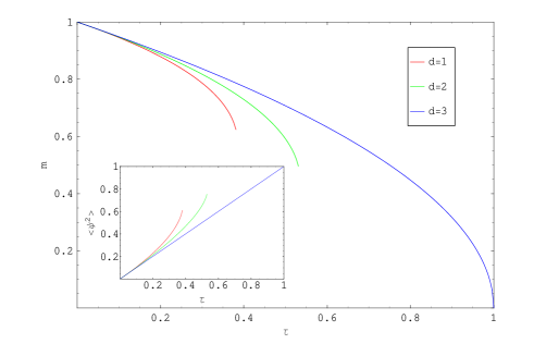
Figure 1: Temperature dependence of the amplitude of the principal mode $m$ for different dimensions. The inset shows the corresponding values of the mean square fluctuations $\left\langle\psi^{2}\right\rangle$.

At this point we have obtained self-consistently the fluctuations for subcritical temperatures from a purely dynamical perspective. We may now analyze the nature of the transition to the modulated phase. From expression (5) it is possible to write the amplitude of the modulation $m$ as a function of $\langle\psi^{2}\rangle$ and thus to obtain the value of $m$ for every temperature in any dimension. It is clear from figure 1 that, for $d\leq 2$, the transition to the high-temperature paramagnetic phase is discontinuous, contrary to $d=3$, where $m$ goes continuously to zero as $\tau$ approaches to $\tau_{c}$. To better realize the consequences of the coupling between modes in our work let’s consider the dynamic calculation in the infinite time limit without the coupling terms in equation (Symmetry breaking in frustrated systems: effective fluctuation spectrum due to coupling effects). In this case the dynamical equation is diagonal and modes with different momentum are not coupled. Following standard procedures, the self-consistent solution to the problem leads to the following equation:

$$\left\langle\Psi^{2}\right\rangle=\frac{T}{(2\pi)^{d}}\int d^{d}k\ \frac{1}{\gamma+\hat{A}(k)},$$ (12)

where $\gamma=-A(k_{0})-3u\left\langle\Psi^{2}\right\rangle$ as before. What we have obtained is a new equation for the square mean fluctuations in which the fluctuation spectrum is spherically symmetric as in the standard Brazovskii-like approaches. The solution to this problem has been obtained many times in the literature Grousson et al. (2002); Tarzia and Coniglio (2007) showing discontinuous transitions to the striped phase. Our new results suggest that the nature of the transition to the modulated phase depends on dimensionality.

Topological properties.- We now focus in the two-dimensional case in order to study the topological order of the modulated phase by means of two parameters commonly used in the literature with this purpose.Nicolao and Stariolo (2007); Quian and Mazenko (2003) The first one is a positional order parameter defined by:

$$M=\left\langle\frac{1}{S}\int d^{2}x\ \phi(\vec{x})\ \mathrm{sin}(\vec{k}_{0}\cdot\vec{x})\right\rangle,$$ (13)

where $S$ is the area of the system. As can be seen, this parameter corresponds to a staggered normalized magnetization which is $1$ only at zero temperature. Orientational order of the stripes can be quantified by means of the parameter

$$Q=\left\langle\int d^{2}x\ \mathrm{cos}(2\theta(\vec{x}))\ \delta(\phi(\vec{x}))\right\rangle/\left\langle\int d^{2}x\ \delta(\phi(\vec{x}))\right\rangle$$ (14)

which again is defined in such a way that is $1$ only in the perfect stripes configuration. Here $\delta(\phi(\vec{x}))=\phi(\vec{x}+\delta\vec{x})-\phi(\vec{x})$.

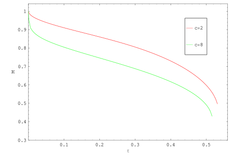
Figure 2: Behavior of $M$ as a function of the reduced temperature for different values of $c$

In order to calculate parameters (13) and (14) we use a gaussian distribution for $\phi$ and its spatial derivatives in the evaluation of the corresponding averages. This assumption is consistent with the Hartree approximation and allows us to find analytically closed expressions that, as far as we know, have never been obtained for topological order parameters. Since the final expressions are not particularly enlightning, we numerically evaluate them under some reasonable approximations. In this context we observe that the positional order parameter only depends on the dimensionless quantity $c=\frac{-A(k_{0})}{k_{0}^{2}}$. In figure 2 we show typical behaviors of this positional parameter. On the other hand, the orientational order parameter depends on $c$ and also on the number $A_{2}$. This dependence is shown in figure 3. As can be expected, the presence of a critical temperature for the two-dimensional system is reflected by means of jumps to zero of both, orientational and positional parameters at $T_{c}$ (figures 2 and 3). Our calculations show that these parameters decrease with increasing $c$, while the increase of $A_{2}$ only causes an increasing of the orientational order. This dependence of order parameters with $A_{2}$ and $c$ reveals a rich topological scenario for the two-dimensional system. In particular, this picture supports the existence of the so-called nematic phase that has been the subject of some debate in the recent literature.Nicolao and Stariolo (2007); Barci and Stariolo (2007); Cannas et al. (2006) This nematic phase is characterized by a strong orientational order in the absence of positional order. Our results suggests that, by appropriately increasing $c$ and $A_{2}$, we may eventually obtain a region of temperatures close to $T_{c}$ in which the orientational order prevails over the positional one. To test this one should have to consider a particular model and its full fluctuation spectrum.

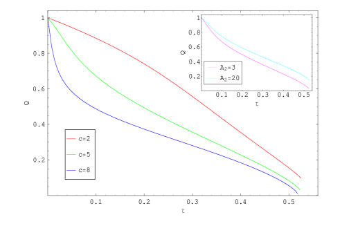
Figure 3: Behavior of $Q$ as a function of the reduced temperature. The main figure corresponds to $A_{2}=3$ and several values of $c$. In the inset $c=5$ and several values of $A_{2}$ were taken.

On the other hand, the existence of a phase in which positional order prevails over orientational one is also suggested. From figure 3 one can see that increasing $c$ the decay of the orientational parameter at low temperatures becomes more abrupt. This fact, together with the decrease of $Q$ for increasing values of $A_{2}$ (inset of figure 3) could be responsible for the appearance of such a phase. One can visualize this state by considering highly irregular stripe borders confined in such a small width that the staggered magnetization $M$ is not too compromised. In that sense the lack of positional order in the nematic phase could be seen as the situation in which this width, that defines the penetration depth of the fluctuations, completely covers the width of the stripes. In this situation, thermal fluctuations are strong enough to break the stripes order generating a configuration with topological defects that, as have been discussed in previous works, may give rise to a nematic phase. Finally, there is an absence of numerical evidence in literature supporting the existence of a phase with positional but not orientational order. This is probably due to the presence of a strong anisotropy, caused by a discretization mesh of the order of the modulation length in numerical works Nicolao and Stariolo (2007); Cannas et al. (2006). In fact, this anisotropy effects favors the emergence of orientational order that makes the nematic phase easier to find.

Conclusions.- Taking the infinite time limit, the steady state properties of a model of competing interactions have been studied from a purely dynamical calculation. Such a procedure makes use of the Hartree approximation over the fluctuations field and the isotropy of the system is explicitly broken. This leads to an effective fluctuation spectrum that is not isotropic anymore, contrary to the one present in Brazovskii-like calculations. Within this formalism, it was possible to analytically obtain the fluctuations as functions of the temperature and thus analyze some interesting parameters in the modulated state. In particular, the first order character suggested in literature for this transition is not verified for the tree-dimensional case, in which a continuous transition takes place due to the coupling between modes. The present approach extends our understanding about the nature of modulated phases in systems with competing interactions. We have also calculated analytically and discussed usual topological observables. Our restuls suggest that, for certain range of temperatures close to the transition, it may exist a nematic phase with purely orientational order, or even a phase in which the translational order prevails over the orientational one, depending on some system dependent parameters. A more detailed paper including the discussion of dynamical observables will be published in short.

We acknowledge useful discussions with D. G. Barci at the early stages of this work. D.A.S. acknowledges partial support from CNPq (Brazil).

References

- Brazovskii (1975) S. A. Brazovskii, Sov. Phys. JEPT 41, 85 (1975).
- Garel and Doniach (1982) T. Garel and S. Doniach, Phys. Rev. B 26, 325 (1982).
- Cannas et al. (2004) S. A. Cannas, D. A. Stariolo, and F. A. Tamarit, Phys. Rev. B 69, 092409 (2004).
- Díaz-Méndez and Mulet (2010) R. Díaz-Méndez and R. Mulet, Phys. Rev. B 81, 184420 (2010).
- Grousson et al. (2001) M. Grousson, G. Tarjus, and P. Viot, Phys. Rev. E 64, 036109 (2001).
- Grousson et al. (2002) M. Grousson, V. Krakoviack, G. Tarjus, and P. Viot, Phys. Rev. E 66, 26126 (2002).
- Abanov et al. (1995) A. Abanov, V. Kalatsky, V. L. Pokrovsky, and W. M. Saslow, Phys. Rev. B 51, 1023 (1995).
- Cannas et al. (2006) S. A. Cannas, M. F. Michelon, D. A. Stariolo, and F. A. Tamarit, Phys. Rev. B 73, 184425 (2006).
- Barci and Stariolo (2007) D. G. Barci and D. A. Stariolo, Phys. Rev. Lett. 98, 200604 (2007).
- Mulet and Stariolo (2007) R. Mulet and D. A. Stariolo, Phys. Rev. B 75, 064108 (2007).
- Tarzia and Coniglio (2007) M. Tarzia and A. Coniglio, Phys. Rev. E 75, 011410 (2007).
- Díaz-Méndez et al. (2010) R. Díaz-Méndez, A. Mendoza, R. Mulet, L. Nicolao, and D. Stariolo, to be published (2010).
- Nicolao and Stariolo (2007) L. Nicolao and D. A. Stariolo, Phys. Rev. B 76, 054453 (2007).
- Quian and Mazenko (2003) H. Quian and G. Mazenko, Phys. Rev. E 67, 036102 (2003).