Persistent current and Drude weight for the one-dimensional Hubbard model from current lattice density functional theory

Abstract

The Bethe-Ansatz local density approximation (LDA) to lattice density functional theory (LDFT) for the one-dimensional repulsive Hubbard model is extended to current-LDFT (CLDFT). The transport properties of mesoscopic Hubbard rings threaded by a magnetic flux are then systematically investigated by this scheme. In particular we present calculations of ground state energies, persistent currents and Drude weights for both a repulsive homogeneous and a single impurity Hubbard model. Our results for the ground state energies in the metallic phase compares favorably well with those obtained with numerically accurate many-body techniques. Also the dependence of the persistent currents on the Coulomb and the impurity interaction strength, and on the ring size are all well captured by LDA-CLDFT. Our study demonstrates that CLDFT is a powerful tool for studying one-dimensional correlated electron systems with high accuracy and low computational costs.

I Introduction

Quantum dots, routinely made by electrostatically confining a two-dimensional electron gas Davies , have been extensively studied in recent years Thierry_book . The interest in these low-dimensional structures stems from the fact that their physics is controlled by quantum effects. Furthermore, while sharing many similarities with real atoms, quantum dots manifest intriguing low-energy quantum phenomena, which are specific to them. This is because their properties can be influenced by external factors such as the geometry or the shape of the confining potential and the application of external fields. Clearly some of these features are not accessible in real atoms. Research in the past has been motivated by the possibility of developing novel quantum dot based devices in both the fields of quantum cryptography/computing Zipper and spintronic Foldi , as well as by the simple curiosity of exploring the properties of many-electron systems in reduced dimensions.

Quantum rings represent a particular class of quantum dots Lorke ; Fuhrer , where electrons are confined in circular regions Garcia ; Lorke2 . The circular geometry can sustain an electrical current, which in turns can be induced by threading a magnetic flux across the ring itself. Such a magnetic flux produces exciting effects like Ahanorov-Bohm (AB) oscillations Aharonov ; Levy and persistent currents Buttiker , effects that were anticipated as early as the late 60’s Bloch1 ; Bloch2 . In one dimension (1D) the persistent currents have been thoroughly studied Buttiker ; Buttiker2 . These, as many other physical properties of the ring, are a periodic function of the magnetic flux quantum, $\Phi_{0}=hc/e$ ($h$ is the Planck’s constant, $c$ the speed of light and $e$ the electron’s charge).

A number of earlier theoretical studies Giancarlo ; Kirchner ; Molina ; SKMaiti2004 ; Thierry2 on persistent currents focused on unveiling the role of electron correlations and disorder over the electron transport. This line of research is inspired by the fact that electronic correlation in 1D always leads to non-fermionic low-energy quasiparticle excitations. In fact, even in the presence of weak interaction, 1D fermions behave differently from a Fermi liquid and their ground state is generally referred to as Luttinger liquid. This possesses specific collective excitations Kolomeisky .

There are two theoretical frameworks commonly used to study finite 1D rings Viefers . The first is based on the continuum model, where electrons move in a uniform neutralizing positive background and interact via Coulomb repulsion, $e^{2}/4\pi\varepsilon_{0}r$ ($\varepsilon_{0}$ is the vacuum permittivity, $e$ the electron charge, $r$ the distance between two electrons). The second is populated by lattice models, where the electronic structure is written in a tight-binding form and the electron-electron interaction is commonly described at the level of Hubbard Hamiltonian Hubbard1 ; Hubbard2 . In both frameworks exact diagonalization (ED) has been the preferential solving strategy for small systems (small number of sites and electrons) SKMaiti2004 ; Bouzerar . Additional methods used to study quantum rings over lattice models include Bethe Ansatz (BA) Bethe ; LiebWu , renormalization group Meden and density matrix renormalization group Dias . In contrast the continuum model has been tackled with self-consistent Hartree Fock techniques Cohen , bosonization schemes Gogolin , conformal field theory Jaimungal , current-spin density functional theory Viefer2 and quantum Monte Carlo Emperador .

Many of the methods developed for solving lattice models for interacting electrons suffer from a number of intrinsic limitations connected either to their large computational overheads or to the need of using a drastically contracted Hilbert space. Density functional theory (DFT) can be a natural solution to these limitations. DFT is a highly efficient and precisely formulated method HK ; KS , originally developed for the Coulomb interaction (this is commonly known as ab initio DFT), and then extended to lattice models Gunnarsson ; Schonhammer ; Capelle3 . Lattice DFT (LDFT) is based on the rigorously proved statement that the ground state of an interacting electron system is a universal functional of the local site occupation. The functional, as in ab initio DFT, is unknown explicitly. However all the many-body contributions to the total energy can be incorporated in a single term, the exchange and correlation (XC) energy, for which a hierarchy of approximations can be constructed.

The most commonly used approximation for the XC energy in ab initio DFT is probably the local density approximation (LDA) KS ; Densityfunctional , where the exact (unknown) XC energy is replaced by that of the homogeneous electron gas. The theory is then expected to work best in situations close to those described by the reference system, i.e. close to the homogeneous electron gas. Since in 1D Fermi liquid theory breaks down, the homogeneous electron gas is no longer a good reference. For the homogeneous Hubbard model it was then proposed Capelle3 ; Capelle1 to use instead the BA construction of Lieb and Wu LiebWu . Such a scheme was then applied successfully to a wide range of situations Capelle2 ; Silva ; Campo ; Xianlong1 ; Xianlong2 ; Xianlong3 ; Akin and more recently it has been extended to time-dependent problems Xianlong3 ; Verdozzi ; Kurth ; Stefanucci and to the 3D Hubbard model Karlsson .

LDFT can be further extended to include the action of a vector potential, i.e. it can be used to tackle problems where a magnetic flux is relevant. This effectively corresponds to the construction of current-LDFT (CLDFT). Such an extension of LDFT was proposed recently for one-dimensional spinless fermions with nearest-neighbor interaction Schenk and it is here adapted to the repulsive Hubbard model. The newly constructed functional is then used to investigate total energies, persistent currents and Drude weights of a mesoscopic repulsive Hubbard ring threaded by a magnetic flux.

The paper is organized as follows. Section II reviews the theoretical foundations leading to the construction of CLDFT and to its LDA. Then we present our results for both homogeneous and defective rings, highlighting the main capabilities and limitations of our scheme, and finally we conclude.

II Theoretical Formulation of Current Lattice DFT

Current-DFT (CDFT) is a generalization of time-dependent density functional theory Gross to include in the Hamiltonian an external vector potential thebook . In this case the theory is constructed over two fundamental quantities, namely the electron density, $n$, and the paramagnetic current density, $\vec{j}_{p}$. The Hohenberg-Kohn theorem HK is thus expanded to the statement that the ground state $n$ and $\vec{j}_{p}$ uniquely determine the ground-state wave-function and consequently the expectation values of all the operators Vignale1 ; Vignale2 . Equally important is the fact that the standard Kohn-Sham construction can also be employed for CDFT, so that the many-body problem can be mapped onto a fictitious single-particle one, with the two sharing the same ground state $n$ and $\vec{j}_{p}$ Vignale1 ; Vignale2 . Practically one then needs to solve self-consistently a system of single-particle equations. Also for CDFT all the unknown of the theory are incorporated in the XC energy, which then needs to be approximated.

The scope of this section is to describe how ab initio CDFT has been translated to lattice models and how a suitable approximation for the XC energy associated to the Hubbard Hamiltonian can be constructed. Our description follows closely the one previously given by Dzierzawa et al. Schenk . In general a vector potential, $\vec{A}$, enters into a lattice model via Peierls substitution Peir ; Vogel , where the matrix elements of the $\vec{A}$-dependent Hamiltonian, $H(\vec{r},\vec{p}+\frac{e}{c}\vec{A})$, can be written in terms of those for $\vec{A}=0$ as

$$\langle\vec{R}^{\prime}|H(\vec{r},\vec{p}+\frac{e}{c}\vec{A})|\vec{R}\rangle=\langle\vec{R}^{\prime}|H(\vec{r},\vec{p})|\vec{R}\rangle\mathrm{e}^{-\frac{ie}{\hbar c}\int_{\vec{R}}^{\vec{R}^{\prime}}\vec{A}\cdot\mathrm{d}\vec{s}}\>,$$ (1)

where $c$ is the speed of light and $|\vec{R}\rangle$ is the generic orbital located at the position $\vec{R}$ and belonging to the basis set (here assumed orthogonal) used to construct the tight-binding Hamiltonian.

When the Peierls substitution is applied to the construction leading to the 1D Hubbard model the only term in the Hamiltonian that gets modified is the kinetic energy $\hat{T}$. This takes the form

$$\hat{T}=-t\sum_{\sigma,\>l=1}^{L}(e^{-i{\Phi_{\sigma l}/L}}\>\hat{c}^{\dagger}_{\sigma\>l+1}\hat{c}_{\sigma\>l}+hc)\>,$$ (2)

where we have considered a system comprising $L$ atomic sites (note that the ring boundary conditions imply $L+1=1$). In the equation (2) $\hat{c}^{\dagger}_{\sigma l}$ ($\hat{c}_{\sigma l}$) is the creation (annihilation) operator for an electron of spin $\sigma$ ($\sigma=\uparrow,\downarrow$) at the $l$-site, $t$ is the hopping integral and $\Phi_{\sigma l}$ is the phase associated to the $l$-th bond, which effectively describes the action of $\vec{A}$. The remaining terms in the Hamiltonian are unchanged so that the 1D Hubbard model in the presence of a vector potential is defined by

$$\hat{H}^{\Phi}_{\mathrm{Hubbard}}=\hat{T}+\hat{U}+\sum_{l}^{L}v_{l}^{\mathrm{ext}}\hat{n}_{l}\>,$$ (3)

where {$v_{l}^{\mathrm{ext}}$} is the external potential ($v_{l}^{\mathrm{ext}}$ is the on-site energy of the $l$-site), while the Coulomb repulsion term is $\hat{U}=U\sum_{l=1}^{L}\hat{n}_{\uparrow l}\hat{n}_{\downarrow l}$, with $U$ being the Coulomb repulsion energy and $\hat{n}_{\sigma l}=\hat{c}^{\dagger}_{\sigma l}\hat{c}_{\sigma l}$. Throughout this work we always consider the diamagnetic (non-spin polarized) case so that $\Phi_{\uparrow l}=\Phi_{\downarrow l}=\Phi_{l}$ and $n_{\uparrow l}=n_{\downarrow l}=n_{l}$.

The first step in the construction of a CLDFT is the formulation of the problem in a functional form. The basic variables of the theory are the site occupation $n_{l}=\langle\Psi|\hat{n}_{l}|\Psi\rangle$ and bond paramagnetic current, $j_{l}=\langle\Psi|\hat{j}_{l}|\Psi\rangle$, where $|\Psi\rangle$ is the many-body wavefunction and the bond paramagnetic current operator is defined as

$$\hat{j}_{l}=-it(e^{-i{\Phi_{l}/L}}\>\hat{c}^{\dagger}_{\sigma\>l+1}\hat{c}_{\sigma\>l}-hc)$$ (4)

In complete analogy to ab initio CDFT we can write the total energy, $\mathcal{E}$, of the Hamiltonian (3) as a functional of the local external potentials and phases

$$\mathcal{E}=\mathcal{F}[n_{l},j_{l}]+\sum_{l}v_{l}^{\mathrm{ext}}n_{l}+\sum_{l}\Phi_{l}j_{l},$$ (5)

so that

$$n_{l}=\langle\hat{n}_{l}\rangle =\frac{\partial\mathcal{E}}{\partial v_{l}^{\mathrm{ext}}}\>,$$ (6)

$$j_{l}=\langle\hat{j}_{l}\rangle =\frac{\partial\mathcal{E}}{\partial\Phi_{l}}\>.$$

$\mathcal{F}[n_{l},j_{l}]$ is a universal functional, whose functional derivatives with respect to $\{n_{l}\}$ and $\{j_{l}\}$ satisfy the following two equations

$$v_{l}^{\mathrm{ext}}= -\frac{\partial\mathcal{F}}{\partial n_{l}}$$ (7)

$$\Phi_{l}= -\frac{\partial\mathcal{F}}{\partial j_{l}}.$$

Note that equations (5) through (7) follow directly from the properties of the Legendre transformation.

In order to make the theory practical one has now to introduce the auxiliary single-particle Kohn-Sham system. This is described by a single-particle Hamiltonian, $\hat{H}^{\mathrm{s}}$, whose ground state site occupations and bond paramagnetic currents are identical to those of the interacting system [described by equation (3)]. $\hat{H}^{\mathrm{s}}$ reads

$$\hat{H}^{\mathrm{s}}=\hat{T}^{\mathrm{s}}+\sum_{l}^{L}v_{l}^{\mathrm{s}}\hat{n}_{l},$$ (8)

where $\hat{T}^{\mathrm{s}}=-t\sum_{\sigma,l=1}^{L-1}(e^{-i{\Phi_{l}^{\mathrm{s}}/L}}\>\hat{c}^{\dagger}_{\sigma\>l+1}\hat{c}_{\sigma l}+hc)$ and the associated local effective potentials and phases are $v_{l}^{\mathrm{s}}$ and $\Phi_{l}^{\mathrm{s}}$ respectively. The single-particle Schrödinger equation is then

$$\hat{H}^{\mathrm{s}}|\Psi^{\mathrm{s}}_{\alpha}\rangle=\epsilon_{\alpha}|\Psi^{\mathrm{s}}_{\alpha}\rangle,$$ (9)

and the site occupation is defined as

$$n_{l}^{\mathrm{s}}=\sum_{\alpha}f_{\alpha}\langle\Psi^{\mathrm{s}}_{\alpha}|\hat{n}_{l}|\Psi^{\mathrm{s}}_{\alpha}\rangle\>,$$ (10)

where $f_{\alpha}$ is the occupation number. An analogous expression can be written for $j^{\mathrm{s}}_{l}$.

The energy functional associated the Kohn-Sham system, $\mathcal{F}^{\mathrm{s}}$, can be constructed by performing again a Legendre transformation

$$\mathcal{F}^{\mathrm{s}}=\mathcal{E}^{\mathrm{s}}-\sum_{l}v_{l}^{\mathrm{s}}n_{l}^{\mathrm{s}}-\sum_{l}\Phi_{l}^{\mathrm{s}}j_{l}^{\mathrm{s}}\>,$$ (11)

where $\mathcal{E}^{\mathrm{s}}$ is the total energy of the single-particle system and the following two equations are valid

$$v_{l}^{\mathrm{s}}= -\frac{\partial\mathcal{F}^{\mathrm{s}}}{\partial n_{l}^{\mathrm{s}}}\>,$$ (12)

$$\Phi_{l}^{\mathrm{s}}= -\frac{\partial\mathcal{F}^{\mathrm{s}}}{\partial j_{l}^{\mathrm{s}}}\>.$$

The crucial point is that in the ground state the real and the Kohn-Sham systems share the same site occupation and paramagnetic current, i.e. $n_{l}=n_{l}^{\mathrm{s}}$ and $j_{l}=j_{l}^{\mathrm{s}}$.

Thus one is now in the position of defining the XC energy, $\mathcal{E}^{\mathrm{xc}}$, as usual, i.e. as the difference between $\mathcal{F}$ for the interacting and the Kohn-Sham systems after the classical Hartree energy $\mathcal{E}^{\mathrm{H}}$ has also been subtracted,

$$\mathcal{E}^{\mathrm{xc}}[n_{l},j_{l}]=\mathcal{F}[n_{l},j_{l}]-\mathcal{F}^{\mathrm{s}}[n_{l},j_{l}]-\mathcal{E}^{\mathrm{H}}[n_{l}]\>.$$ (13)

Note that for all the functionals in equation (13) we took the short notation $\{n_{l}\}\rightarrow n_{l}$ and $\{j_{l}\}\rightarrow j_{l}$, i.e. the functionals depend on all the on-site occupations and bond paramagnetic currents. The single-particle effective potentials and phases can now be defined. In fact by taking the functional derivative of equation (13) with respect to $n_{l}$ and $j_{l}$ and by using the equations (7) and (12) one obtains

$$v_{l}^{\mathrm{s}}= v_{l}^{\mathrm{ext}}+v_{l}^{\mathrm{H}}+v_{l}^{\mathrm{xc}}\>,$$ (14)

$$\Phi_{l}^{\mathrm{s}}= \Phi_{l}+\Phi_{l}^{\mathrm{xc}}\>,$$

where

$$v_{l}^{\mathrm{xc}}= \frac{\partial\mathcal{E}_{l}^{\mathrm{xc}}}{\partial n_{l}}\>,$$ (15)

$$\Phi_{l}^{\mathrm{xc}}= \frac{\partial\mathcal{E}_{l}^{\mathrm{xc}}}{\partial j_{l}}\>,$$

and $v_{l}^{\mathrm{H}}=\partial\mathcal{E}_{l}^{\mathrm{H}}/\partial n_{l}$ ($=Un_{l}/2$) is the Hartree potential.

Finally $\mathcal{E}^{\mathrm{xc}}$ can be re-written in terms of the expectation values of the original Hamiltonian. In fact by substituting the functional forms of $\mathcal{F}$ and $\mathcal{F}^{\mathrm{s}}$ into the equation (13),

$$\mathcal{E}^{\mathrm{xc}}=\mathcal{E}-\mathcal{E}^{\mathrm{s}}+\sum_{l}(v_{l}^{\mathrm{s}}-v_{l}^{\mathrm{ext}})n_{l}+\sum_{l}(\Phi_{l}^{\mathrm{s}}-\Phi_{l})j_{l}-\mathcal{E}^{\mathrm{H}}[n_{l}]\>,$$ (16)

by using the equations (3) and (8),

$$\sum_{l}(v_{l}^{\mathrm{s}}-v_{l}^{\mathrm{ext}})n_{l}=\mathcal{E}^{\mathrm{s}}-\mathcal{E}-\langle\Psi^{\mathrm{s}}|\hat{T}^{\mathrm{s}}|\Psi^{\mathrm{s}}\rangle+\langle\Psi|\hat{T}+\hat{U}|\Psi\rangle\>,$$ (17)

and again by substituting equation (17) into equation (16), one obtains a close expression for the XC energy

$$\mathcal{E}^{\mathrm{xc}}=\langle\Psi|\hat{T}+\hat{U}|\Psi\rangle-\langle\Psi^{\mathrm{s}}|\hat{T}^{\mathrm{s}}|\Psi^{\mathrm{s}}\rangle+\sum_{l}(\Phi_{l}^{\mathrm{s}}-\Phi_{l})j_{l}-\mathcal{E}^{\mathrm{H}}[n_{l}].$$ (18)

Once the theory is formally established the remaining task is that of finding an appropriate approximation for $\mathcal{E}^{\mathrm{xc}}$. As for the case of standard LDFT Capelle1 ; Capelle2 , the strategy here is that of considering the BA solution for the homogeneous limit of $\hat{H}^{\Phi}_{\mathrm{Hubbard}}$ (this is defined in equation (3) by setting $v_{l}=v$ and $\Phi_{l}=\Phi$) and then of taking its local density approximation $n\rightarrow n_{l}$, $\Phi\rightarrow\Phi_{l}$ Schenk , i.e.

$$\mathcal{E}^{\mathrm{xc}}_{\mathrm{LDA}}[n_{l},j_{l}]=\sum_{l}e^{\mathrm{xc}}[n_{l},j_{l}],$$ (19)

where $e^{\mathrm{xc}}[n,j]={\mathcal{E}^{\mathrm{xc}}[n,j]/L}$ is the XC energy density (per site) of the homogeneous system. The first term of the equation (18) can be calculated exactly using the BA procedure Shastry . This provides the ground state energy as a function of $n$ and $\Phi$, so that one still needs to re-express it in terms of $n$ and $j$. However the phase variable $\Phi$ can be eliminated from the ground state energy by using

$$j=\frac{\partial\mathcal{E}(n,\Phi)}{\partial\Phi}\>.$$ (20)

Thus finally one can explicitly write $e^{\mathrm{xc}}(n,j)$ (the full derivation for the 1D Hubbard Hamiltonian is presented in the Appendix)

$$e^{\mathrm{xc}}(n,j)=e^{\mathrm{xc}}(n,0)+\frac{1}{2}\Lambda^{\mathrm{xc}}(n)j^{2},$$ (21)

where

$$e^{\mathrm{xc}}(n,0)= \frac{\mathcal{E}^{\mathrm{BA}}(n,0)-\mathcal{E}^{0}(n,0)-\mathcal{E}^{\mathrm{H}}(n)}{L}\>,$$ (22)

$$\Lambda^{\mathrm{xc}}(n)= \frac{1}{2}\left[\frac{1}{D_{c}^{0}(n)}-\frac{1}{D_{c}^{\mathrm{BA}}(n)}\right].$$

In the equations above $\mathcal{E}^{0}(n,0)$ and $D_{c}^{0}(n)$ are respectively the non-interacting ground state energy and charge stiffness, while $\mathcal{E}^{\mathrm{BA}}(n,0)$ and $D_{c}^{\mathrm{BA}}(n)$ are the same quantities for the interacting case as calculated from the BA. Finally, the XC contributions to the Kohn-Sham potential can be obtained by simple functional derivative (in this case by simple derivative) of the exchange and correlation energy density with respect to the fundamental variables $n$ and $j$, i.e.

$$v^{\mathrm{xc}}_{\mathrm{BALDA}}(n_{l},j_{l})=\left.\frac{\partial e^{\mathrm{xc}}(n,j)}{\partial n}\right|_{n\rightarrow n_{l},j\rightarrow j_{l}}\>,$$ (23)

and

$$\Phi^{\mathrm{xc}}_{\mathrm{BALDA}}(n_{l},j_{l})=\left.\frac{\partial e^{\mathrm{xc}}(n,j)}{\partial j}=\Lambda^{\mathrm{xc}}(n)j\right|_{n\rightarrow n_{l},j\rightarrow j_{l}}\>,$$ (24)

where BALDA, as usual, stands for Bethe Ansatz local density approximation.

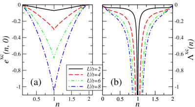
Figure 1: (Color online) The XC energy density (per site) for a homogeneous 1D Hubbard ring threaded by a magnetic flux as a function of the electron density and for different values of interaction strength $U/t$: (a) $e^{xc}(n,0)$ and (b) $\Lambda^{xc}(n)$.

In the two panels of figure 1 we present $e^{\mathrm{xc}}(n,0)$ and $\Lambda^{\mathrm{xc}}(n)$ as a function of the electron density, $n$, for different interaction strengths $U/t$. As in the case of standard LDFT also for CLDFT there is a divergence in the $n$-derivative of both $e^{\mathrm{xc}}(n,0)$ and $\Lambda^{\mathrm{xc}}(n)$ at half-filing ($n=1$). This is in correspondence of the metal-insulator-transition present in the 1D Hubbard model for finite $U/t$. In the case of $\Lambda^{\mathrm{xc}}(n)$ the divergence is also in $\Lambda^{\mathrm{xc}}(n)$ itself.

The solution of the Kohn-Sham problem proceeds as follows. First an initial guess for the site occupations is used to construct the initial local paramagnetic current density. Then, the functional derivatives of equations (23) and (24) are evaluated at these given $n$ and $j$ so that the Kohn-Sham potential is constructed. The Kohn-Sham equations are then solved to obtain the new set of Kohn-Sham orbitals from which the new orbital occupations and bond paramagnetic currents are calculated [by using equation (10)]. The procedure is then repeated untill self-consistency is reached, i.e. until the potentials (or the densities) at two consecutive iterations vary below a certain threshold. After convergence is achieved the total energy for the interacting system is calculated from

$$\mathcal{E}=\sum_{\alpha}f_{\alpha}\epsilon_{\alpha}+\mathcal{E}^{\mathrm{xc}}[n_{l},j_{l}]-\mathcal{E}^{\mathrm{H}}[n_{l}]-\sum_{l}v_{l}^{\mathrm{xc}}n_{l},$$ (25)

where the first term is the sum of single-particle energies and the other terms are the so-called double counting corrections.

III Results and Discussion

We now discuss how CLDFT performs in describing both the energetics and the transport properties of 1D Hubbard rings in presence of a magnetic flux. For small rings our results will be compared with those obtained by diagonalizing exactly the Hamiltonian of equation (3), while CLDFT for large rings will be compared with the BA solution. First we will consider homogeneous rings and then we will explore the single impurity problem.

III.1 Homogeneous rings: general properties

In this section we focus our attention on discussing the general features of CLDFT applied to homogeneous Hubbard rings threatened by a magnetic flux, i.e. on the performance of CLDFT in describing the Ahanorov-Bohm effect. We start our analysis by comparing the CLDFT results with those obtained by ED. Since ED is numerically intensive such a comparison is limited to small systems.

In figure 2 we present the first low-lying energy levels, $\mathcal{E}$, calculated by ED as a function of the magnetic flux, $\Phi$, for a small 12-site ring at quarter filling ($n=1/2$). In particular we present results for the non-interacting case [panel (a)] and for the interacting one at three different interaction strengths: (b) $U/t=2$, (c) $U/t=4$ and (d) $U/t=6$. Exact results (ED) are in black, while those obtained with CLDFT in red. In general the ground state energy is mimimized at $\Phi=0$ when the number of electrons is $N=4m+2$ and at $\Phi=\pi$ for $N=4m$, with $m$ being an integer Nakano . Here we consider the case $N=4m+2$ where the ground state is a singlet Stafford .

For non-interacting electrons, $U/t=0$, the total energy of the singlet ground state is a parabolic function of $\Phi$. Also the various excited states have a parabolic dependence on $\Phi$ and simply correspond to single-particle levels with different wave-vectors.

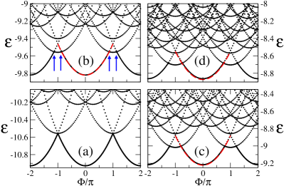
Figure 2: (Color online) The low lying energy spectrum, $\mathcal{E}$, of a 12-site ring at quarter filling ($n=1/2$) as a function of the magnetic flux, $\Phi$, and calculated for different interaction strengths $U/t$. The black dotted lines represent ED results while the dashed red ones are for CLDFT. Note that for the non interacting case, $U/t=0$, in panel (a) there is no difference between CLDFT and ED. Panels (b)-(d) are for the interacting case at different interaction strengths: (b) $U/t=2$, (c) $U/t=4$ and (d) $U/t=6$. In panel (b) the blue arrows indicate the region where the triplet state becomes the ground state.

As the electron-electron interaction is turned on the non-interacting spectrum gets modified in two ways. Firstly there is a second branch in the ground state energy as a function of $\Phi$ appearing at around $\Phi=\pm\pi$ (see the blue arrows in panel (b) of Fig. 2). This originates from the degeneracy lifting between the single and the triplet solution at $\Phi=\pm\pi$, with the triplet being pushed down in energy and becoming the ground state. The $\Phi$ region where the ground state is a triplet widens as the interaction strengths increases. The second effect is the expected reduction of the ground state total energy as a function of $U/t$.

Since CLDFT is a ground state theory, it provides access only to the ground state energy, $\mathcal{E}$. This is calculated next and plotted in figure 2 in the interval $-\pi\leq\Phi\leq\pi$ for different $U/t$. As one can clearly see from the figure the performance of CLDFT is rather remarkable, to a point that the CLDFT energy is practically identical to that calculated with ED. However CLDFT completely misses the cusps in the $\mathcal{E}(\Phi)$ profile arising from the crossover between the singlet and the triplet state. Level crossing invalidates the BA approximation leading to the interacting XC energy [see equation (36) in the appendix] and so failures are expected Romer . This observation is in agreement with earlier studies Viefers in which the inability of CDFT to reproduce level crossing was already noted. Nevertheless, as long as the singlet remains the ground state, the agreement between CLDFT and ED results is remarkable, even if this small ring is rather far from being a good approximation of the thermodynamic limit (the BA solution) upon which the functional has been constructed.

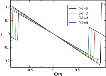
Figure 3: (Color online) Persistent current profile, $j$, for a 12-site ring at quarter filling ($n=1/2$) obtained with both ED and CLDFT for different $U/t$. The full lines are the $j$ calculated with ED while the dashed ones are for CLDFT.

Having calculated the total energies with both ED and CLDFT, the corresponding persistent currents, $j$, can be obtained by taking the numerical derivative of $\mathcal{E}(\Phi)$ with respect to $\Phi$. In figure 3 we show results for the 12 site ring at quarter filling ($n=1/2$), whose total energy was presented in figure 2. In particular we plot $j$ only over the period $-\pi<\Phi<\pi$, since all the quantities are 2$\pi$ periodic. The figure confirms the linearity of the persistent currents with the magnetic flux for all the interaction strengths considered. The same is also true for other fillings for the 12 site ring (not presented here) away from half-filling. We also observe that the magnitude of persistent currents reduces with increasing $U/t$ for both ED and CLDFT and that the precise dependence of $j$ on $U/t$ is different for different fillings. This is in good agreement with previous calculations based on the BA technique BoBo .

ED is computationally demanding and cannot be performed beyond a certain system size. For this reason, in order to benchmark CLDFT for larger rings, we have calculated the ground state energy with the BA method. An example of these calculations is presented in figure 4, where once again we show $\mathcal{E}(\Phi)$ for $L=20$, $U/t=4$ and different numbers of electrons. Also in this case the agreement between the BA results and those obtained with CLDFT is remarkably good as long as the ground state is a singlet. Interestingly we note that the agreement is better for low filling but it deteriorates as one approaches the half-filling case ($N=20$ in this case). This is somehow expected given the discontinuity of $\Lambda^{\mathrm{xc}}$ and of the derivative of $e^{\mathrm{xc}}$ at $n=1$ (see figure 1), leading to the Mott transition. The presence of these discontinuities, although qualitatively correct, poses numerical problems and losses in accuracy.

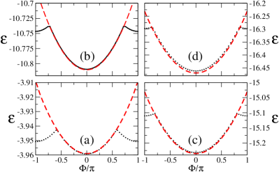
Figure 4: (Color online) Ground state energy, $\mathcal{E}(\Phi)$, as a function of the magnetic flux, $\Phi$, calculated with both the BA technique (dotted black line) and CLDFT (dashed red line). Calculations are carried out for $L=20$, $U/t=4$ and different numbers of electrons: (a) $N=2$ ($n=1/10$), (b) $N=6$ ($n=0.3$), (c) $N=10$ ($n=1/2$) and (d) $N=14$ ($n=0.7$).

The final quantity we wish to consider is the charge stiffness or Drude weight, $D_{\mathrm{c}}$, defined as

$$D_{\mathrm{c}}=\frac{L}{2}\frac{\partial^{2}\mathcal{E}(n,\Phi)}{\partial\Phi^{2}}|_{\Phi=0}\>.$$ (26)

This is essentially the slope of the persistent current as a function of $\Phi$ calculated at $\Phi=0$ and defines the magnitude of the real part of the optical conductivity in the long wave-length limit (see appendix for more details). $D_{\mathrm{c}}$ determines both qualitatively and quantitatively the transport properties of the ring. Importantly in the limit of large rings it exponentially vanishes for insulators, while it saturates to a finite value for metals. Many studies have been devolved to calculating $D_{\mathrm{c}}$ for interacting systems. Römer and Punnoose have studied $D_{\mathrm{c}}$ for finite Hubbard rings using an iterative BA technique Romer . Eckern et. al. explored the relation between $D_{\mathrm{c}}$ and the so-called phase sensitivity, $\Delta\mathcal{E}$, for spinless fermions. $\Delta\mathcal{E}$ is the difference in the total energy calculated at $\Phi=0$ (periodic ground state) and that at $\Phi=\pi$ (antiperiodic ground state) Schenk1 ; Schmitteckert . Recently a density matrix renormalization group algorithm has been developed to deal with complex Hamiltonian matrices and used to calculate $D_{\mathrm{c}}$ for spinless fermions Dias .

Since the agreement between CLDFT and ED is proved for small rings (the slopes of the persistent currents as a function of $\Phi$ calculated with CLDFT and ED are essentially identical in figure 3) we concentrate here on a larger system, namely a homogeneous 60 site ring at quarter filling. Our results for the Drude weight as a function of $U/t$ are presented in figure 5. Again the CLDFT data are compared with those calculated with the BA in the thermodynamic limit ($L\rightarrow\infty$) and the agreement is rather satisfactory. We note that, as for the ground state energy, also for the Drude weight the CLDFT seems to perform less well as $U/t$ increases, i.e. as the interaction strength becomes large.

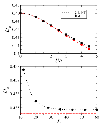
Figure 5: (Color online) Drude coefficient $D_{\mathrm{c}}$ as a function of the interaction strength $U/t$ (top panel) and of the number of sites in the ring, $L$ (bottom panel). All the calculations are for quarter filling and the results in the top panel are for a 60-site ring. In the figure we compare CLDFT results (dotted black lines) with those obtained by the BA technique in the thermodynamic limit (dashed red lines). Calculations in the lower panel are for $U/t=2$.

Then in the lower panel of figure 5 we illustrate the scaling properties of $D_{\mathrm{c}}$ as a function of the number of sites in the ring, $L$ (we consider quarter filling and $U/t=2$). Clearly $D_{\mathrm{c}}$ does not vanish at any lengths demonstrating that the system remains metallic. Furthermore it approaches a constant value already for $L>40$. In the picture we also report the asymptotic value predicted by the BA in the thermodynamic limit $L\rightarrow\infty$ for this set of parameters. We find that the calculated CLDFT value is only 0.06% larger than the BA one, i.e. it is in quite remarkable good agreement.

III.2 Scaling properties

Next we take a more careful look at the scaling properties of the persistent currents and the Drude weights as a function of both the ring size and the interaction strength. It is well known that $j$ is strongly size dependent, since it originates from electron coherence across the entire ring Dias . For a perfect metal one expect $j$ to scale as $1/L$ Bouzerar . In Figure 6 the value of the persistent currents as a function of the ring size are presented for different electron fillings and for the two representative interaction strengths of $U/t=2$ (a) and $U/t=4$ (b). Calculations are performed with both the exact BA and CLDFT. As a matter of convention we calculate the persistent currents at $\Phi=\pi/2$.

In general we find a monotonic reduction of the persistent current with $L$ and an overall excellent agreement between the BA and the CLDFT results over the entire range of lengths, occupations and interaction strengths investigated.

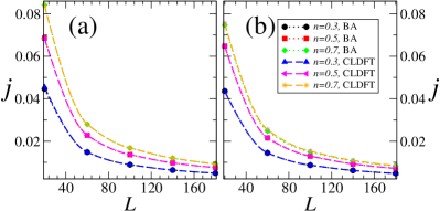
Figure 6: (Color online) Persistent current, $j$, as a function of the number of site in the ring, $L$, and for different electron occupations, $n$: (a) $U/t=2$, (b) $U/t=4$. Results are obtained with both the exact BA technique and CLDFT. In the figure the persistent currents are calculated at $\Phi=\pi/2$, i.e. $j=j(\pi/2)$

A non-linear fit of all the curves of figure 6 returns us an almost perfect $1/L$ dependence of $j$ with no appreciable deviations at any $n$ or $U/t$. This indicates a full metallic response of the rings in the region of parameters investigated, thus confirming previous results obtained with the BA approach BoBo .

Then we look at the dependance of $j$ and $D_{\mathrm{c}}$ on the interaction strength. In this case we consider a 60 site ring and three different different electron fillings. In general for small fluxes one expects $j=2D_{\mathrm{c}}\Phi$ and our numerical results of Fig. 7 demonstrates that this is approximately correct also for our definition of persistent currents [$j=j(\Phi=\pi/2)$] over the entire $U/t$ range investigated.

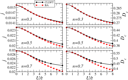
Figure 7: (Color online) Persistent current, $j$, and Drude weight, $D_{\mathrm{c}}$ as a function of interaction strength $U/t$ for a 60 site ring at different fillings. Results are obtained with both the exact BA technique and CLDFT.

We find that both $j$ and $D_{\mathrm{c}}$ monotonically decrease as a function of the interaction strength, essentially meaning that the predicted long-wavelength optical conductivity is reduced as the electron repulsion gets larger.

Also in this case the agreement between the BA and the CLDFT results is substantially good, although significant deviations appear in the limit of large $U/t$ and electron filling approaching half-filling. This again corresponds to a region of the parameter space where the XC potential approaches the derivative discontinuity.

It was numerically demonstrated in the past BoBo that the persistent current (and so the Drude weight) at half-filling follows the scaling relation $j\sim\mathrm{e}^{-U^{2}/\xi}$, with $\xi\sim 1$. However, to the best of our knowledge, no scaling relation was ever provided in the metallic case. We have then carried out a fitting analysis (the fit is limited to values of $j$ and $D_{\mathrm{c}}$ for $U/t>2$) and found that our data can be well represented by the scaling lows

$$j=j_{0}(U/t)^{-\beta},\;\;\;\;\;\;\;D_{\mathrm{c}}=D_{0}(U/t)^{-\gamma}\>.$$ (27)

In general and as expected we find $\beta=\gamma$ and a quite significant dependence of the exponents on the filling. In particular table 1 summarizes our results and demonstrates that the decay rate of both the persistent currents and the Drude weights increases as the filling approaches half-filling. Furthermore the table also quantifies the differences between the BA and the CLDFT solutions, whose exponents increasingly differ from each other as the electron filling gets closer to $n=1$ (for $n=0.7$ we find $\beta^{\mathrm{BA}}\sim 2\beta^{\mathrm{CLDFT}}$).

$n$	$\beta^{\mathrm{CLDFT}}$	$\beta^{\mathrm{BA}}$
0.3	0.036	0.036
0.5	0.085	0.104
0.7	0.151	0.246

Table 1: Exponents for the empirical scaling laws of equation (27) as fitted from the data of figure 7.

Finally, by combining all the results of this section we can propose a scaling law for both the persistent currents and the Drude weights, valid in the metallic limit of the Hubbard model, i.e. away from half-filling. This reads

$$j=\frac{j_{0}(n)}{L}\left(\frac{U}{t}\right)^{-\beta(n)}\>,$$ (28)

where both the constant $j_{0}$ and the exponent $\beta$ are function of the electron filling $n$. Note that an identical equation holds for $D_{\mathrm{c}}$.

III.3 Scattering to a single impurity

Having established the success of the BALDA to CLDFT for the homogeneous case we now move to a more stringent test for the theory, namely the case of a ring penetrated by a magnetic flux in the presence of a single impurity. Such a problem has already received considerable attention in the past Viefer2 ; Koskinen ; Cheung . Note that, as in ab initio DFT, this is a situation different from the reference system used to construct the BALDA (since it deals with a non homogeneous system) and therefore one might expect a more pronounced disagreement with exact results. As the BA equations are integrable only for the homogeneous case we now benchmark our CLDFT results with those obtained by ED. This however limits our analysis to small rings.

The single impurity in the ring is described by simply adding to the Hamiltonian of equation (3) the term

$$\hat{H}_{\mathrm{imp}}= \varepsilon_{\mathrm{imp}}\hat{n}_{i}\>,$$ (29)

where $\varepsilon_{\mathrm{imp}}$ is the modification to the on-site energy at the impurity site $i$. The inclusion of an impurity produces in general electron backscattering so that we expect the persistent currents to get reduced. In figure 8 we present the general transport features for this inhomogeneous system. Calculations have been carried out with CLDFT for a ring comprising 53 sites and $N=26$, $U/t=4$. Again the persistent currents are calculated at $\Phi=\pi/2$.

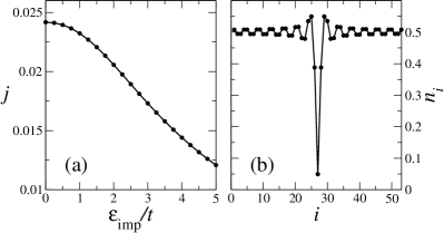
Figure 8: (a) Persistent current, $j$, as a function of single impurity strength, $\varepsilon_{\mathrm{imp}}$, obtained from the CLDFT for $L=53$, $N=26$, $U/t=4$ and $\Phi=\frac{\pi}{2}$. In (b) we show a typical site density profile for a positive single impurity site potential.

Panel (a) shows $j$ as a function of the impurity on-site energy. As expected from standard scattering theory the current is reduced as $\varepsilon_{\mathrm{imp}}$ increases, thus creating a potential barrier. The electron density profile for this situation is presented in panel (b), where one can clearly observe an electron depletion at the impurity site and Friedel’s oscillations around it.

A quantitative assessment of our CLDFT results is provided in Fig. 9 where they are compared with those obtained by exact diagonalization for a 13 site ring close to quarter filling ($N=6$). In particular we present $j$ as a function of the impurity potential, $\varepsilon_{\mathrm{imp}}$, for both $U/t=2$ and $U/t=4$. In general we find a rather satisfactory agreement between CLDFT and the exact results in particular for small $\varepsilon_{\mathrm{imp}}$ and $U/t$. As the electron scattering becomes more significant deviations appear and the quantitative agreement is less good. Importantly we notice that the ED results systematically provide a persistent current lower than that calculated with CLDFT, at least for the values of electron filling investigated here. This seems to be a consistent trend also present for the homogeneous case (see figure 7), although the deviations in that case are less pronounced (for the same electron filling and interaction strength). Therefore we tentatively conclude that most of the errors in the impurity problem have to be attributed to the errors already present in the homogeneous case. We then expect that CLDFT provides a good platform for investigating scattering problems at only minor computational costs. As such CLDFT appears as the ideal tool for investigating the interplay between electron-electron interaction and disorder in low dimensional structures.

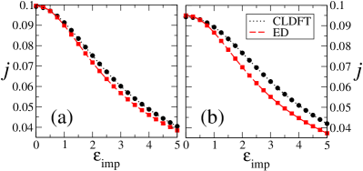
Figure 9: (Color on line) Comparison between the persistent currents calculated with CLDFT (black symbols and dotted line) and by ED (red symbols and dashed line) for a 13 site ring and $N=6$. The $j$’s are obtained at $\Phi=\pi/2$ for two different values of the interaction strength, namely $U/t=2$ (a) and $U/t=4$ (b).

IV Conclusion

In this work we have presented an extension of the BALDA for the one-dimensional Hubbard problem on a ring to CLDFT. We have then investigated the response of interacting rings to an external flux both in the homogeneous and inhomogeneous case, and we have compared our results with those obtained by numerically exact techniques. Our analysis has been confined to the metallic limit, i.e. away from half-filling, where the Hubbard model has a metal to insulator transition. In general we have found that CLDFT performs rather well in calculating both the persistent currents and the Drude weights in the homogeneous case. Furthermore a similar level of accuracy is transferred to the impurity problem. With these results in hands we propose to use CLDFT in the study of AB rings where the combined effect of electron-electron interaction and disorder can be addressed for large rings, so that a numerical evaluation of the various scaling laws proposed in the past can be accurately carried out.

V Acknowledgements

We thank N. Baadji, I. Rungger and V. L. Campo for useful discussions. This work is supported by Science Foundation of Ireland under the grant SFI05/RFP/PHY0062 and 07/IN.1/I945. Computational resources have been provided by the HEA IITAC project managed by the Trinity Center for High Performance Computing and by ICHEC.

VI APPENDIX: Local Density Approximation for the CLDFT

We use the BA solution for the homogeneous part of the $\hat{H}_{U}^{\Phi}$ [equation (3)] to estimate the XC energy. Then the local approximation is taken,

$$\mathcal{E}^{\mathrm{xc}}_{\mathrm{LDA}}[n_{l},j_{l}]=\sum_{l}e^{\mathrm{xc}}[n_{l},j_{l}]\>.$$ (30)

Here $e^{\mathrm{xc}}(=\frac{\mathcal{E}^{\mathrm{xc}}[n,j]}{L})$ is the XC energy per site for the homogeneous system, which is provided in equation (18). The first term of the equation (18) can be calculated exactly using the BA procedures Shastry to obtain the ground state energy as a function of $n$ and $\Phi$. Then the phase variable $\Phi$ can be eliminated from the ground state energy to contain the current via

$$j=\frac{\partial\mathcal{E}(n,\Phi)}{\partial\Phi}\>.$$ (31)

The complete flux dependence of the ground state energy for the Mott insulator phase ($n=1$) in the thermodynamic limit has been shown to be Stafford

$$\mathcal{E}(n,\Phi)-\mathcal{E}(n,0)=\frac{2D_{c}(n)}{L}(1-\cos\Phi)\>,$$ (32)

while away from half filling and $L\rightarrow\infty$ this is

$$\mathcal{E}(n,\Phi)-\mathcal{E}(n,0)=\frac{D_{\mathrm{c}}(n)}{L}\Phi^{2}\>.$$ (33)

Here $D_{\mathrm{c}}(n)$ is the charge stiffness (Drude weight) defined as

$$D_{\mathrm{c}}=\left.\frac{L}{2}\frac{\partial^{2}\mathcal{E}(n,\Phi)}{\partial\Phi^{2}}\right|_{\Phi=0}.$$ (34)

In physical terms the Drude weight $D_{\mathrm{c}}$ is the real part of the optical conductivity $\sigma_{1}(w)$ in the long wavelength limit Stafford ,

$$\sigma_{1}(w)=2\pi D_{\mathrm{c}}\delta(w)+\sigma_{1}^{\text{reg}}(w)\>,$$ (35)

where we took $\hbar=e=c=1$. If we denote $\mathcal{E}^{\mathrm{BA}}(n_{\mathrm{BA}},\Phi_{\mathrm{BA}})$ and $\mathcal{E}^{0}(n_{0},\Phi_{0})$ respectively as the ground state energy for the interacting system [first term in equation (18)] and for the non-interacting one [second term in equation (18)], away from half-filling we will write

$$\mathcal{E}^{\mathrm{BA}}(n_{\mathrm{BA}},\Phi_{\mathrm{BA}})= \mathcal{E}^{\mathrm{BA}}(n_{\mathrm{BA}},0)+\frac{D_{\mathrm{c}}^{\mathrm{BA}}(n_{\mathrm{BA}})}{L}\Phi^{2}_{\mathrm{BA}}\>,$$ (36)

$$\mathcal{E}^{0}(n_{0},\Phi_{0})= \mathcal{E}^{0}(n_{0},0)+\frac{D_{c}^{0}(n_{0})}{L}\Phi^{2}_{0}\>,$$

and

$$j^{\mathrm{BA}}(n_{\mathrm{BA}},\Phi_{\mathrm{BA}})= 2\frac{D_{\mathrm{c}}^{\mathrm{BA}}(n_{\mathrm{BA}})}{L}\Phi_{\mathrm{BA}}\>,$$ (37)

$$j^{0}(n_{0},\Phi_{0})= 2\frac{D_{c}^{0}(n_{0})}{L}\Phi_{0}\>.$$

The fundamental requirement of the KS mapping is that $n_{\mathrm{BA}}=n_{0}=n$ and $j^{\mathrm{BA}}=j^{0}=j$ while we note that $\Phi_{\mathrm{BA}}=\Phi$ and $\Phi_{0}=\Phi^{s}$ in equation (18). By substituting equation (36) and the expressions for $\Phi^{s}$ and $\Phi$ obtained from equation (37) into equation (18) one obtains

$$\mathcal{E}^{\mathrm{xc}}(n,j)=\mathcal{E}^{\mathrm{BA}}(n,0)-\mathcal{E}^{0}(n,0)-\mathcal{E}^{\mathrm{H}}(n)+\frac{L}{2}\Lambda^{\mathrm{xc}}(n)j^{2},$$ (38)

where

$$\Lambda^{\mathrm{xc}}(n)=\frac{1}{2}\left[\frac{1}{D_{\mathrm{c}}^{0}(n)}-\frac{1}{D_{\mathrm{c}}^{\mathrm{BA}}(n)}\right].$$ (39)

Here $D_{\mathrm{c}}^{0}(n)$ is the non-interacting charge stiffness defined as

$$D_{\mathrm{c}}^{0}(n)=\frac{2t}{\pi}\sin\left(\frac{n\pi}{2}\right)$$ (40)

for $L\rightarrow\infty$. $D_{\mathrm{c}}^{\mathrm{BA}}(n)$ can then be obtained in the thermodynamic limit by using Kawakami

$$D_{\mathrm{c}}^{\mathrm{BA}}(n)=\frac{1}{2\pi}[\xi_{\mathrm{c}}(Q)]^{2}v_{\mathrm{c}}$$ (41)

where $\xi_{\mathrm{c}}$ is an element of the dressed charge matrix, which is used to describe the scattering between the quasi-particles and $v_{\mathrm{c}}$ is velocity of the charge excitation. Therefore one finally obtains

$$e^{\mathrm{xc}}(n,j)=e^{\mathrm{xc}}(n,0)+\frac{1}{2}\Lambda^{\mathrm{xc}}(n)j^{2},$$ (42)

so that

$$v^{\mathrm{xc}}_{\mathrm{BALDA}}(n_{l},j_{l})=\left.\frac{\partial e^{\mathrm{xc}}(n,j)}{\partial n}\right|_{n\rightarrow n_{l},j\rightarrow j_{l}},$$ (43)

and

$$\Phi^{\mathrm{xc}}_{\mathrm{BALDA}}(n_{l},j_{l})=\left.\frac{\partial e^{\mathrm{xc}}(n,j)}{\partial j}=\Lambda^{\mathrm{xc}}(n)j\right|_{n\rightarrow n_{l},j\rightarrow j_{l}}.$$ (44)

References

- (1) J.H. Davies, The Physics of Low-Dimensional Semiconductor, (Cambridge University Press, Cambridge, 1998).
- (2) See for example T. Giamarchi, Quantum Physics in One Dimension, First Edition, (Oxford University Press, 2004).
- (3) E. Zipper, M. Kurpas, M. Szelag, J. Dajka and M. Szopa, Phys. Rev B 74, 125426 (2006).
- (4) P. Földi, O. Kálmán, M.G. Benedict and F.M. Peeters, Phys. Rev. B 73, 155325 (2006).
- (5) A. Lorke, R. J. Luyken, A.O. Govorov, J.P. Kotthaus, J.M. Garcia and P.M. Petroff, Phys. Rev. Lett. 84, 2223 (1999)
- (6) A. Fuhrer, S. Lüsher, T. Ihn, T. Heinzel, K. Ensslin, W. Wegscheider and M. Bichler, Nature (London) 413, 822 (2001)
- (7) J.M. Garcia, G. Medeiros-Ribeiro, K. Schmidt, T. Ngo, J.L. Feng, A.Lorke, J. Kotthaus and P.M. Petroff, Appl. Phys. Lett. 71, 2014 (1997).
- (8) A. Lorke and R. J. Luyken, Physica B 256, 424 (1998).
- (9) Y. Aharonov and D. Bohm, Phys. Rev. 115, 485, (1959).
- (10) L.P. Levy, G. Dolan, J. Dunsmuir and H. Bouchiat, Phys. Rev. Lett. 64, 2074 (1990).
- (11) M. Büttiker, Y. Imry and R. Landauer, Phys. Lett. A 96, 365 (1983).
- (12) F. Bloch, Phys. Rev. 137, A787 (1965).
- (13) F. Bloch, Phys. Rev. 166, 415 (1968).
- (14) M. Büttiker, Phys. Rev. B 32, 1846(R) (1985).
- (15) G. Queeroz-Pallegrino, J. Phys.: Condens. Matter 13 8121 (2001).
- (16) S. Kirchner, H.G. Evertz and W. Hanke, PRB 59 1825 (1999).
- (17) R.A. Molina, D. Weinmann, R.A. Jalabert, G. Ingold and J. Pichard, Phys. Rev. B 67 235306 (2003).
- (18) S.K. Maiti, J. Chowdhury and S.N. Karmakar Phys. Lett. A 332 497 (2004).
- (19) T. Giamarchi and B. Sriram Shastry, Phys. Rev. B. 51, 10915 (1995).
- (20) E.B. Kolomeisky and J.P. Straley, Rev. Mod. Phys. 68, 175 (1996).
- (21) S. Viefers, P. Koskinen, P. Singha Deo and M. Manninen, Physica E 21, 1 (2004).
- (22) J. Hubbard, Proc. Roy. Soc. A 276, 238 (1963).
- (23) J. Hubbard, Proc. Roy. Soc. A 277, 237 (1964).
- (24) G. Bouzerar, D. Poiblanc and G. Montambaux, Phys. Rev. B 49, 8258 (1994).
- (25) H.A. Bethe, Z. Phys. 71, 205 (1931).
- (26) E.H. Lieb and F.Y. Wu, Phys. Rev. Lett. 20, 1445 (1968), E. H. Lieb and F. Y. Wu, Physica A 321, 1 (2003).
- (27) V. Meden and U. Schollwöck, Phys. Rev. B 67, 035106 (2003).
- (28) F.C. Dias, I.R. Pimentel and M. Henkel, Phys. Rev. B 73, 075109 (2006).
- (29) A. Cohen, K. Richter and R. Berkovits, Phys. Rev. B 57, 6223 (1998).
- (30) A.O. Gogolin and N.V. Prokof’ev, Phys. Rev. B 50, 4921 (1994).
- (31) S. Jaimungal, M.H.S. Amin and G. Rose, Int. J. Mod. Phys. B 13, 3171 (1999)
- (32) S. Viefers, P. Singha Deo, S.M. Reimann, M. Manninen and M. Koskinen, Phys. Rev. B 62, 10668 (2000).
- (33) F. Pederiva, A. Emperador and E. Lipparini, Phys. Rev. B 66, 165314 (2002).
- (34) P. Hohenberg and W. Kohn, Phys. Rev. 136, B864 (1964).
- (35) W. Kohn and L.J. Sham, Phys. Rev. 140, A1133 (1965).
- (36) O. Gunnarsson and K. Schonhammer, Phys. Rev. Lett. 56, 1968 (1986).
- (37) K. Schonhammer, O. Gunnarsson and R.M. Noack, Phys. Rev. B. 52, 2504 (1995).
- (38) K. Capelle, N.A. Lima, M.F. Silva and L.N. Oliviera, in The Fundamentals of Electron Density, Density Matrix and Density Functional theory in Atoms, Molecules and Solids, Kluwer series, “Progress in Theoretical Chemistry and Physics,” edited by N. I. Gidopoulos and S. Wilson (Kluwer, Dordrecht, 2003).
- (39) Density functionals: Theory and Applications, edited by D. Joulbert, Springer Lecture Notes in Physics Vol. 500 (Springer, Berlin, 1998).
- (40) N.A. Lima, L.N. Oliviera and K. Capelle, Euro. Phys. Lett. 60, 601 (2002).
- (41) N.A. Lima, L.N. Oliviera and K. Capelle, Phys. Rev. Lett. 90, 146402 (2003).
- (42) M.F. Silva, N.A. Lima, A.L. Malvezzi and K. Capelle, Phys. Rev. B. 71, 125130 (2005).
- (43) V. L. Campo, Jr. and K. Capelle, Phys. Rev. A. 72, 061602(R) (2005).
- (44) G. Xianlong, M. Polini, M.P. Tosi, V.L. Campo, K. Capelle and M. Rigol, Phys. Rev. B. 73, 165120 (2006).
- (45) G. Xianlong, M. Rizzi, M. Polini, R. Fazio, M.P. Tosi, V.L. Campo and K. Capelle, Phys. Rev. Lett. 98, 030404 (2007).
- (46) W. Li, G. Xianlong, C. Kollath and M. Polini, Phys. Rev. B. 78, 195109 (2008).
- (47) A. Akande and S. Sanvito, Phys. Rev. B 82 245114 (2010).
- (48) C. Verdozzi, Phys. Rev. Lett. 101, 166401 (2008).
- (49) S. Kurth, G. Stefanucci, E. Khosravi, C. Verdozzi and E.K.U. Gross, Phys. Rev. Lett. 104, 236801 (2010).
- (50) S. Kurth and G. Stefanucci, arXiv:1012.4296
- (51) D. Karlson, A. Privitera and C. Verdozzi, arXiv:1004.2264 (2010).
- (52) M. Dzierzawa, U. Eckern, S. Schenk, and P. Schwab, Phys. Status Solidi B 246, 941 (2009).
- (53) E. Runge and E.K.U. Gross, Phys. Rev. Lett. 52, 997 (1984).
- (54) G. F. Giuliani and G. Vignale, Quantum Theory of the Electron Liquid, (Cambridge University Press, Cambridge (UK), 2005).
- (55) G. Vignale and M. Rasolt, Phys. Rev. Lett. 59, 2360 (1987).
- (56) G. Vignale and M. Rasolt, Phys. Rev. B. 37, 10685 (1988).
- (57) R. Peierls, Z. Phys. 80, 763 (1933).
- (58) M. Graf and P. Vogl, Phys. Rev. B 51, 4940 (1995).
- (59) B.S. Shastry and B. Sunderland, Phys. Rev. Lett. 65, 243 (1990).
- (60) F. Nakano, J. Phys. A: Math. Gen. 33, 5429 (2000).
- (61) C.A. Stafford and A.J. Millis, Phys. Rev. B 48, 1409 (1993).
- (62) R.A. Römer and A. Punnoose, Phys. Rev. B 52, 14809 (1995).
- (63) B.-B. Wei, S.-J. Gu and H.-Q. Lin, J. Phys.: Condens. Matter 20, 395209 (2008).
- (64) S. Schenk, M. Dzierzawa, P. Schwab and U. Eckern, Phys. Rev. B. 78, 165102 (2008).
- (65) P. Schmitteckert, T. Schulze, C. Schuster, P. Schwab and U. Eckern, Phys. Rev. Lett. 80, 560 (1998).
- (66) P. Koskinen and M. Manninen, Phys. Rev. B. 68, 195304 (2003).
- (67) H-F. Cheung, Y. Gefen, E.K. Riedel and W.H. Shih, Phys. Rev. B 37, 6050 (1988).
- (68) N. Kawakami and S.-K. Yang, Phys. Rev. B 44, 7844 (1991).