Affine-invariant geodesic geometry of deformable 3D shapes

Abstract

Natural objects can be subject to various transformations yet still preserve properties that we refer to as invariants. Here, we use definitions of affine invariant arclength for surfaces in ${\mathbb{R}}^{3}$ in order to extend the set of existing non-rigid shape analysis tools. In fact, we show that by re-defining the surface metric as its equi-affine version, the surface with its modified metric tensor can be treated as a canonical Euclidean object on which most classical Euclidean processing and analysis tools can be applied. The new definition of a metric is used to extend the fast marching method technique for computing geodesic distances on surfaces, where now, the distances are defined with respect to an affine invariant arclength. Applications of the proposed framework demonstrate its invariance, efficiency, and accuracy in shape analysis.

1 Introduction

Modeling 3D shapes as Riemannian manifold is a ubiquitous approach in many shape analysis applications. In particular, in the recent decade, shape descriptors based on geodesic distances induced by a Riemannian metric have become popular. Notable examples of such methods are the canonical forms [7] and the Gromov-Hausdorff [9, 13, 2] and the Gromov-Wasserstein [12] frameworks, used in shape comparison and correspondence problems. Such methods consider shapes as metric spaces endowed with a geodesic distance metric, and pose the problem of shape similarity as finding the minimum-distortion correspondence between the metrics. The advantage of the geodesic distances is their invariance to inelastic deformations (bendings) that preserve the Riemannian metric, which makes them especially appealing for non-rigid shape analysis. A particular setting of finding shape self-similarity can be used for intrinsic symmetry detection in non-rigid shapes [17, 23, 11, 22].

The flexibility in the definition of the Riemannian metric allows extending the invariance of the aforementioned shape analysis algorithms by constructing a geodesic metric that is also invariant to global transformations of the embedding space. A particularly general and important class of such transformations are the affine transformations, which play an important role in many applications in the analysis of images [14] and 3D shapes [8]. Many frameworks have been suggested to cope with the action of the affine group in a global manner, trying to undo the affine transformation in large parts of a shape or a picture. While the theory of affine invariance is known for many years [4] and used for curves [18] and flows [19], no numerical constructions applicable to manifolds have been proposed.

In this paper, we construct an (equi-)affine-invariant Riemannian geometry for 3D shapes. By defining an affine-invariant Riemannian metric, we can in turn define affine-invariant geodesics, which result in a metric space with a stronger class of invariance. This new metric allows us to develop efficient computational tools that handle non-rigid deformations as well as equi-affine transformations. We demonstrate the usefulness of our construction in a range of shape analysis applications, such as shape processing, construction of shape descriptors, correspondence, and symmetry detection.

2 Background

We model a shape $(X,g)$ as a compact complete two-dimensional Riemannian manifold $X$ with a metric tensor $g$. The metric $g$ can be identified with an inner product $\langle\cdot,\cdot\rangle_{x}:T_{x}X\times T_{x}X\rightarrow\mathbb{R}$ on the tangent plane $T_{x}X$ at point $x$. We further assume that $X$ is embedded into ${\mathbb{R}}^{3}$ by means of a regular map $\mathbf{x}:U\subseteq{\mathbb{R}}^{2}\rightarrow{\mathbb{R}}^{3}$, so that the metric tensor can be expressed in coordinates as

$$g_{ij}=\frac{\partial\mathbf{x}^{\mathrm{T}}}{\partial u_{i}}\frac{\partial\mathbf{x}}{\partial u_{j}},$$ (1)

where $u_{i}$ are the coordinates of $U$.

The metric tensor relates infinitesimal displacements in the parametrization domain $U$ to displacement on the manifold

$$dp^{2}=g_{11}{du_{1}}^{2}+2g_{12}du_{1}du_{2}+g_{22}{du_{2}}^{2}.$$ (2)

This, in turn, provides a way to measure length structures on the manifold. Given a curve $C:[0,T]\rightarrow X$, its length can be expressed as

$$\ell(C) = \int_{0}^{T}\langle\dot{C}(t),\dot{C}(t)\rangle^{1/2}_{C(t)}dt,$$ (3)

where $\dot{C}$ denotes the velocity vector.

2.1 Geodesics

Minimal geodesics are the minimizers of $\ell(C)$, giving rise to the geodesic distances

$$d_{X}(x,x^{\prime})=\min_{C\in\Gamma(x,x^{\prime})}\ell(C)$$ (4)

where $\Gamma(x,x^{\prime})$ is the set of all admissible paths between the points $x$ and $x^{\prime}$ on the surface $X$, where due to completeness assumption, the minimizer always exists.

Structures expressible solely in terms of the metric tensor $g$ are called intrinsic. For example, the geodesic can be expressed in this way. The importance of intrinsic structures stems from the fact that they are invariant under isometric transformations (bendings) of the shape. In an isometrically bent shape, the geodesic distances are preserved – a property allowing to use such structures as invariant shape descriptors [7].

2.2 Fast marching

The geodesic distance $d_{X}(x_{0},x)$ can be obtained as the viscosity solution to the eikonal equation $\|\nabla d\|_{2}=1$ with boundary condition at the source point $d(x_{0})=0$. In the discrete setting, a family of algorithms for finding the viscosity solution of the discretized eikonal equation by simulated wavefront propagation is called fast marching methods [21, 10]. On a discrete shape represented as a triangular mesh with $N$ vertices, the general structure of fast marching closely resembles that of the classical Dijkstra’s algorithm for shortest path computation in graphs, with the main difference in the update step. Unlike the graph case where shortest paths are restricted to pass through the graph edges, the continuous approximation allows paths passing anywhere in the mesh triangles. For that reason, the value of $d(x_{0},x)$ has to be computed from the values of the distance map at two other vertices forming a triangle with $x$. Computation of the distance map from a single source point has the complexity of $\mathcal{O}(N\log N)$.

3 Affine-invariant geometry

An affine transformation $\mathbf{x}\mapsto\mathbf{A}\mathbf{x}+\mathbf{b}$ of the three-dimensional Euclidean space can be parametrized using twelve parameters: nine for the linear transformation $\mathbf{A}$, and additional three, $\mathbf{b}$, for a translation, which we will omit in the following discussion. Volume-preserving transformations, known as special or equi-affine are restricted by $\det\mathbf{A}=1$. Such transformations involve only eleven parameters.

The equi-affine metric can be defined through the parametrization of a curve on the surface [1, 3, 4, 6, 15, 19]. Let $C$ be a curve on $X$ parametrized by $p$. By the chain rule,

$$\frac{dC}{dp} = \mathbf{x}_{1}\frac{du_{1}}{dp}+\mathbf{x}_{2}\frac{du_{2}}{dp}$$ (5)

$$\frac{d^{2}C}{dp^{2}} = \mathbf{x}_{1}\frac{d^{2}u_{1}}{dp^{2}}+\mathbf{x}_{2}\frac{d^{2}u_{2}}{dp^{2}}+\mathbf{x}_{11}\left(\frac{du_{1}}{dp}\right)^{2}+2\mathbf{x}_{12}\frac{du_{1}}{dp}\frac{du_{2}}{dp}+\mathbf{x}_{22}\left(\frac{du_{2}}{dp}\right)^{2},$$

where, for brevity, we denote $\mathbf{x}_{i}=\frac{\partial\mathbf{x}}{\partial u_{i}}$ and $\mathbf{x}_{ij}=\frac{\partial^{2}\mathbf{x}}{\partial u_{i}\partial u_{j}}$. As volumes are preserved under the equi-affine group of transformations, we define the invariant arclength $p$ through

$$f(X)\det(\mathbf{x}_{1},\mathbf{x}_{2},C_{pp}) = 1,$$ (6)

where $f(X)$ is a normalization factor for parameterization invariance. Plugging (3) into (6) yields

$$dp^{2} = f(X)\det(\mathbf{x}_{1},\mathbf{x}_{2},\mathbf{x}_{11}du_{1}^{2}+2\mathbf{x}_{12}du_{1}du_{2}+\mathbf{x}_{22}du_{2}^{2})$$ (7)

$$= f(X)\left(\tilde{g}_{11}du_{1}^{2}+2\tilde{g}_{12}du_{1}u_{2}+\tilde{g}_{22}du_{2}^{2}\right).$$

where $\tilde{g}_{ij}=\det(\mathbf{x}_{1},\mathbf{x}_{2},\mathbf{x}_{ij})$.

In order to evaluate $f(X)$ such that the quadratic form (7) will also be parameterization invariant, we introduce an arbitrary parameteriation $\bar{u}_{1}$ and $\bar{u}_{2}$, for which $\bar{\mathbf{x}}_{i}=\frac{\partial\mathbf{x}}{\partial\bar{u}_{i}}$ and $\bar{\mathbf{x}}_{ij}=\frac{\partial^{2}\mathbf{x}}{\partial\bar{u_{i}}\partial\bar{u}_{j}}$. The relation between the two sets of parameterizations can be expressed using the chain rule

$$\bar{X}_{1}=X_{\bar{u}_{1}}=X_{u_{1}}{u_{1}}_{\bar{u}_{1}}+X_{u_{2}}{u_{2}}_{\bar{u}_{1}}$$ (8)

$$\bar{X}_{2}=X_{\bar{u}_{2}}=X_{u_{1}}{u_{1}}_{\bar{u}_{2}}+X_{u_{2}}{u_{2}}_{\bar{u}_{2}}.$$

It can shown [4] using the Jacobian

$$J=\begin{pmatrix}{u_{1}}_{\bar{u}_{1}}&{u_{2}}_{\bar{u}_{1}}\\ {u_{1}}_{\bar{u}_{2}}&{u_{2}}_{\bar{u}_{2}}\end{pmatrix},$$ (9)

that

$$\bar{g}_{11}d\bar{u}_{1}^{2}+2\bar{g}_{12}d\bar{u}_{1}d\bar{u}_{2}+\bar{g}_{22}d\bar{u}_{2}^{2}=\left(\tilde{g}_{11}du^{2}+2\tilde{g}_{12}dudv+\tilde{g}_{22}dv^{2}\right)|J|,$$ (10)

and $\bar{g}_{11}\bar{g}_{22}-\bar{g}_{12}^{2}=\left(\tilde{g}_{11}\tilde{g}_{22}-\tilde{g}_{12}^{2}\right)^{4}$, where $\bar{g}_{ij}=\det(\bar{\mathbf{x}}_{1},\bar{\mathbf{x}}_{2},\bar{\mathbf{x}}_{ij})$. From (10) we evaluate the affine invariant parameter normalization $f(X)=\left|\bar{g}\right|^{-1/4}$, and define an equi-affine pre-metric tensor [4, 19]

$$\hat{g}_{ij} = \bar{g}_{ij}\left|\bar{g}\right|^{-1/4}.$$ (11)

The pre-metric tensor (11) defines a true metric only for strictly convex surfaces [4]; A simialr problem appeared in equi-affine curve evolution where the flow direction was determined by the curvature vector. In two dimentions we can encounter non-positive definite metrics in concave, and hyperbolic points. We propose fixing the metric by flipping the main axes of the operator, if needed. In practice we restrict the eigenvalues of the tensor to be positive, and re-avaluate it. From the eigendecomposition $\hat{\mathbf{G}}=\mathbf{U}\mathbf{\Gamma}\mathbf{U}^{\mathrm{T}}$ of $\hat{g}$ in matrix notation, where $\mathbf{U}$ is orthonormal and $\mathbf{\Gamma}=\mathrm{diag}\{\gamma_{1},\gamma_{2}\}$, we compose a new metric $\mathbf{G}$, such that $\mathbf{G}=\mathbf{U}|\mathbf{\Gamma}|\mathbf{U}^{\mathrm{T}}$ is positive definite and equi-affine invariant.

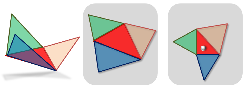
Figure 1: The three neighboring triangles together with the central one are unfolded flat to the plane. The central triangle is canonized into a right isosceles triangle while the rest of its three neighboring triangles follow the same planar affine transformation. Finally, the six surface coordinate values at the vertices are used to interpolate a quadratic surface patch from which the metric tensor is computed.

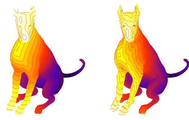
Figure 2: Geodesic level sets of the distance function computed from the tip of the tail, using the standard (left) and the proposed equi-affine (right) geodesic metrics.

Standard                                    Equi-affine

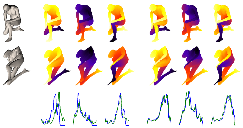
Standard                                    Equi-affine

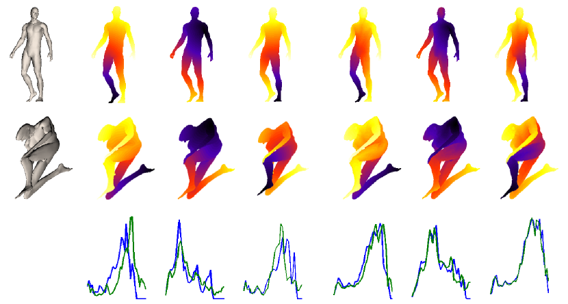
Figure 3: Distance maps from different source points calculated using the standard (second to fourth columns) and the proposed equi-affine geodesic metric (fifth to seventh columns) on a reference surface (first and third rows) and its affine (second row) and isometric deformation+affine transformation (fourth row). Thirds and sixth rows show the global histogram of geodesic distances before and after the transformation (green and blue curves). The overlap between the histograms is an evidence of invariance.

4 Discretization

We model the surface $X$ as a triangular mesh, and construct three coordinate functions $x(u,v)$, $y(u,v)$, and $z(u,v)$ for each triangle. While this can be done practically in any representation, we use the fact that a triangle and its three adjacent neighbors, can be unfolded to the plane, and produce a parameter domain. The coordinates of this planar representation are used as the parametrization with respect to which the first fundamental form coefficients are computed at the barycenter of the simplex (Figure 1). Using the six base functions $1$, $u$, $v$, $uv$, $u^{2}$ and $v^{2}$ we can construct a second order polynom for each coordinate function. This step is performed for every triangle of the mesh.

Calculating geodesic distances was well studied in past decades. Several fast and accurate numerical schemes [10, 20, 24] can be used off-the-shelf for this purpose. We use FMM technique, after locally rescaling each edge according to the equi-affine metric.

The (affine invariant) length of each edge is defined by $L^{2}(dx,dy)=g_{11}dx^{2}+2g_{12}dxdy+g_{22}dy^{2}.$ Specifically, for our canonical triangle with vertices at $(0,0),(1,0)$ and $(0,1)$ we have

$$L^{2}_{1} = g_{11}(1-0)^{2}+2g_{12}(1-0)(0-0)+g_{22}(0-0)^{2}$$ (12)

$$= g_{11}$$ (13)

$$L^{2}_{2} = g_{11}(0-0)^{2}+2g_{12}(0-0)(1-0)+g_{22}(1-0)^{2}$$ (14)

$$= g_{22}$$ (15)

$$L^{2}_{3} = g_{11}(1-0)^{2}+2g_{12}(0-1)(1-0)+g_{22}(1-0)^{2}$$ (16)

$$= g_{11}-2g_{12}+g_{22}.$$ (17)

Each edge may appear in more than one triangle. We found that the average length is a good approximation, assuming the triangle inequality holds. In figures 2 and 3 we compare between geodesic distances induced by the standard and our affine-invariant metric.

5 Results

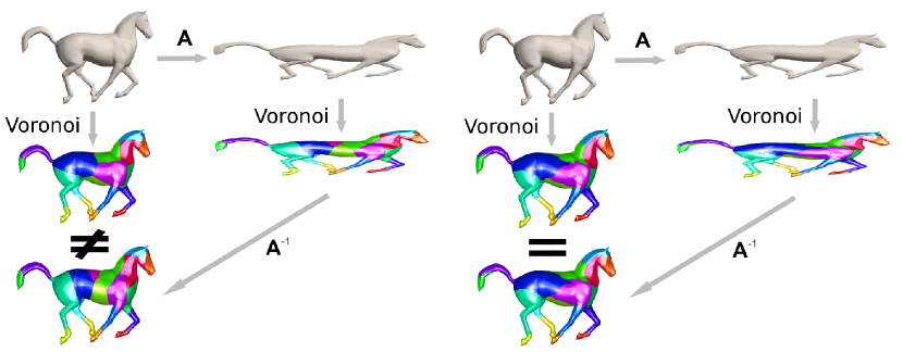
Figure 4: Voronoi cells generated by a fixed set of $20$ points on a shape undergoing an equi-affine transformation. The standard geodesic metric (left) and its equi-affine counterpart (right) were used. Note that in the latter case the tessellation commutes with the transformation.

The equi-affine metric can be used in many existing methods that process geodesic distances. In what follows, we show several examples for embedding the new metric in known applications such as voronoi tessellation, canonical forms, non-rigid matching and symmetry detection.

5.1 Voronoi tessellation

Voronoi tessellation is a partitioning of $(X,g)$ into disjoint open sets called Voronoi cells. A set of $k$ points $\left(x_{i}\in X\right)_{i=1}^{k}$ on the surface define the Voronoi cells $\left(V_{i}\right)_{i=1}^{k}$ such that the $i$-th cell contains all points on $X$ closer to $x_{i}$ than to any other $x_{j}$ in the sense of the metric $g$. Voronoi tessellations created with the equi-affine metric commute with equi-affine transformations as visualized in Figure 4.

5.2 Canonical forms

Methods considering shapes as metric spaces with some intrinsic (e.g. geodesic) distance metric is an important class of approaches in shape analysis. Geodesic distances are particularly appealing due to their invariance to inelastic deformations that preserve the Riemannian metric.

Elad and Kimmel [7] proposed a shape recognition algorithm based on embedding the metric structure of a shape $(X,d_{X})$ into a low-dimensional Euclidean spaces. Such a representation, referred to as canonical form, reduces the number of degress of freedom by tanslating all deformations into a much simple Euclidean isometry group.

Given a shape sampled at $N$ points and an $N\times N$ matrix of pairwise geodesic distances, the computation of the canonical form consists of finding a configuration of $N$ points $z_{1},\ldots,z_{N}$ in ${\mathbb{R}}^{m}$ such that $\|z_{i}-z_{j}\|_{2}\approx d_{X}(x_{i},x_{j})$. This problem is known as multidimensional scaling (MDS) and can be posed as a non-convex least-squares optimization problem of the form

$$\{z_{1},\ldots,z_{N}\} = \mathop{\mathrm{argmin}}_{z_{1},\ldots,z_{N}}\sum_{i>j}|\|z_{i}-z_{j}\|_{2}-d_{X}(x_{i},x_{j})|^{2}.$$ (18)

The invariance of the canonical form to shape transformations depends on the choice of the distance metric $d_{X}$. Figure 5 shows an example of a canonical form of the human shape undergoing different bendings and affine transformations of varying strength. The canonical form was computed using the geodesic and the proposed equi-affine distance metric. One can clearly see the nearly perfect invariance of the latter. Such a strong invariance allows to compute correspondence of full shapes under a combination of inelastic bendings and affine transformations.

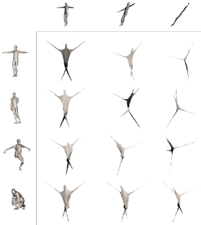
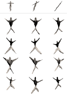
Figure 5: Embedding into $\mathbb{R}^{3}$ of a human shape and its equi-affine transformations of varying strength. Classical scaling was used with a matrix of geodesic (left) and equi-affine geodesic (right) distances. In the latter case, canonical forms remain approximately invariant up to a rigid transformation.

5.3 Non rigid matching

Two non-rigid shapes $X,Y$ can be considered similar if there exists an isometric correspondence $\mathcal{C}\subset X\times Y$ between them, such that $\forall x\in X$ there exists $y\in Y$ with $(x,y)\in\mathcal{C}$ and vice-versa, and $d_{X}(x,x^{\prime})=d_{Y}(y,y^{\prime})$ for all $(x,y),(x^{\prime},y^{\prime})\in\mathcal{C}$, where $d_{X},d_{Y}$ are geodesic distance metrics on $X,Y$. In practice, no shapes are truly isometric, and such a correspondence rarely exists; however, one can attempt finding a correspondence minimizing the metric distortion,

$$\mathrm{dis}(\mathcal{C})=\mathop{\max_{(x,y)\in\mathcal{C}}}_{(x^{\prime},y^{\prime})\in\mathcal{C}}|d_{X}(x,x^{\prime})-d_{Y}(y,y^{\prime})|.$$ (19)

The smallest achievable value of the distortion is called the Gromov-Hausdorff distance [5] between the metric spaces $(X,d_{X})$ and $(Y,d_{Y})$,

$$d_{\mathrm{GH}}(X,Y)=\frac{1}{2}\inf_{\mathcal{C}}\mathrm{dis}(\mathcal{C}),$$ (20)

and can be used as a criterion of shape similarity.

The choice of the distance metrics $d_{X},d_{Y}$ defines the invariance class of this similarity criterion. Using geodesic distances, the similarity is invariant to inelastic deformations. Here, we use geodesic distances induced by our equi-affine Riemannian metric tensor, which gives additional invariance to affine transformations of the shape.

Bronstein et al. [2] showed how (20) can be efficiently approximated using an optimization algorithm in the spirit of multidimensional scaling (MDS), referred to as generalized MDS (GMDS). Since the input of this numeric framework are geodesic distances between mesh points, all is needed to obtain an equi-affine GMDS is one additional step where we substitute the geodesic distances with their equi-affine equivalents. Figure 6 shows the correspondences obtained between an equi-affine transformation of a shape using the standard and the equi-affine-invariant versions of the geodesic metric.

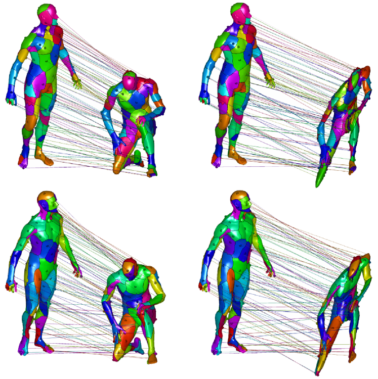
Figure 6: The GMDS framework is used to calculate correspondences between a shape and its isometry (left) and isometry followed by an equi-affine transformation (right). Matches between shapes are depicted as identically colored Voronoi cells. Standard distance (first row) and its equi-affine-invariant counterpart (second row) are used as the metric structure in the GMDS algorithm. Inaccuracies obtained in the first case are especially visible in the legs and arms.

5.4 Intrinsic symmetry

Raviv et al. [17] introduced the notion of intrinsic symmetries for non-rigid shapes as self-isometries of a shape with respect to a deformation-invariant (e.g. geodesic) distance metric. These self-isometries can be detected by trying to identify local minimizers of the metric distortion or other methods proposed in follow-up publications [16, 23, 11, 22].

Here, we adopt the framework of [17] for equi-affine intrinsic symmetry detection. Such symmetries play an important role in paleontological applications [8]. Equi-affine intrinsic symmetries are detected as local minima of the distortion, where the equi-affine geodesic distance metric is used. Figure 7 shows that using the traditional metric we face a decrease in accuracy of symmetry detection as the affine transformation becomes stronger (the accuracy is the average geodesic mismatch with relation to the ground-truth symmetry). Such a decrease does not occur using the equi-affine metric.

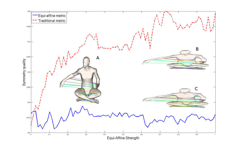
Figure 7: As the affine transformation becomes stronger, the quality of the symmetry detection decreases (B) when the standard geodesic metric is used. On the other hand, detection quality is hardly affected (C) by the transformations when using the equi-affine geodesic metric.

6 Conclusions

We introduced a numerical machinery for computing equi-affine-invariant geodesic distances. The proposed tools were applied to applications, like symmetry detection, finding correspondence, and canonization for efficient shape matching. We have extended the ability to analyze approximately isometric objects, like articulated objects, by treating affine deformations as well as non-rigid ones. As our analysis is based on local geometric structures, the affine group could in fact act locally and vary smoothly in space as long as it is encapsulated within our approximation framework. We intend to explore this direction and further enrich the set of transformations one can handle within the scope of metric geometry in the future.

7 Acknowledgements

This research was supported in part by The Israel Science Foundation (ISF) grant number 623/08, and by the USA Office of Naval Research (ONR) grant.

References

- [1] L. Alveraz, F. Guichard, P. L. Lions, and J. M. Morel. Axioms and fundamental equations of image processing. Archive for Rational Mechanics and Analysis, 123(3):199–257, 1993.
- [2] A. Bronstein, M. Bronstein, and R. Kimmel. Efficient computation of isometry-invarient distances between surfaces. SIAM journal Scientific Computing, 28/5:1812–1836, 2006.
- [3] A. M. Bruckstein and D. Shaked. On projective invariant smoothing and evolutions of planarcurves and polygons. Journal of Mathematical Imaging and Vision, 7:225–240, June 1997.
- [4] S. Buchin. Affine differential geometry. Beijing, China: Science Press, 1983.
- [5] D. Burago, Y. Burago, and S. Ivanov. A course in metric geometry, volume 33 of Graduate studies in mathematics. American Mathematical Society, 2001.
- [6] V. Caselles and C. Sbert. What is the best causal scale space for 3d images? SIAM Journal Applied Math., (56):1196–1246, 1996.
- [7] A. Elad and R. Kimmel. On bending invariant signatures for surfaces. IEEE Trans. on Pattern Analysis and Machine Intelligence (PAMI), 25(10):1285–1295, 2003.
- [8] D. Ghosh, N. Amenta, and M. Kazhdan. Closed-form blending of local symmetries. In Proc. SGP, 2010.
- [9] M. Gromov. Structures Métriques Pour les Variétés Riemanniennes. Number 1 in Textes Mathématiques. 1981.
- [10] R. Kimmel and J. A. Sethian. Computing geodesic paths on manifolds. Proc. National Academy of Sciences (PNAS), 95(15):8431–8435, 1998.
- [11] R. Lasowski, A. Tevs, H. Seidel, and M. Wand. A Probabilistic Framework for Partial Intrinsic Symmetries in Geometric Data. In Proc. International Conference on Computer Vision (ICCV), 2009.
- [12] F. Mémoli. Spectral gromov-wasserstein distances for shape matching. In Proc. NORDIA, 2009.
- [13] F. Mémoli and G. Sapiro. A theoretical and computational framework for isometry invariant recognition of point cloud data. Foundations of Computational Mathematics, 5:313–346, 2005.
- [14] K. Mikolajczyk, T. Tuytelaars, C. Schmid, A. Zisserman, J. Matas, F. Schaffalitzky, T. Kadir, and L. V. Gool. A comparison of affine region detectors. IJCV, 65(1–2):43–72, 2005.
- [15] P. Olver, G. Sapiro, and A. Tennenbaum. Invariant geometric evolutions of surfaces and volumetric smoothing. SIAM Journal Applied Math., (57):176–194, 1997.
- [16] M. Ovsjanikov, J. Sun, and L. Guibas. Global intrinsic symmetries of shapes. In Proc. Eurographics Symposium on Geometry Processing (SGP), volume 27, 2008.
- [17] D. Raviv, A. M. Bronstein, M. M. Bronstein, and R. Kimmel. Symmetries of non-rigid shapes. In Proc. Non-rigid Registration and Tracking (NRTL) workshop. See Proc. of International Conference on Computer Vision (ICCV), Oct. 2007.
- [18] G. Sapiro and A. Tannenbaum. On affine plane curve evolution. Journal of Functional Analysis, (1):79–120, January 1994.
- [19] N. Sochen. Affine-invariant flows in the Beltrami framework. Journal of Mathematical Imaging and Vision, 20(1):133–146, 2004.
- [20] V. Surazhsky, T. Surazhsky, D. Kirsanov, S. Gortler, and H. Hoppe. Fast exact and approximate geodesics on meshes. In Proc. SIGGRAPH, pages 553–560, 2005.
- [21] J. N. Tsitsiklis. Efficient algorithms for globally optimal trajectories. IEEE Trans. Automatic Control, 40(9):1528–1538, 1995.
- [22] K. Xu, H. Zhang, A. Tagliasacchi, L. Liu, G. Li, M. Meng, and Y. Xiong. Partial intrinsic reflectional symmetry of 3d shapes. In Proc. SIGGRAPH Asia, 2009.
- [23] X. Yang, N. Adluru, L. Latecki, X. Bai, and Z. Pizlo. Symmetry of Shapes Via Self-similarity. In Proc. International Symposium on Advances in Visual Computing, pages 561–570, 2008.
- [24] L. Yatziv, A. Bartesaghi, and G. Sapiro. O(N) implementation of the fast marching algorithm. J. Computational Physics, 212(2):393–399, 2006.