The upper atmosphere of the exoplanet HD 209458 b revealed by the sodium D lines

Abstract

A complete reassessment of the Hubble Space Telescope (HST) observations of the transits of the extrasolar planet HD 209458 b has provided a transmission spectrum of the atmosphere over a wide range of wavelengths. Analysis of the NaI absorption line profile has already shown that the sodium abundance has to drop by at least a factor of ten above a critical altitude. Here we analyze the profile in the deep core of the NaI doublet line from HST and high–resolution ground–based spectra to further constrain the vertical structure of the HD 209458 b atmosphere.

With a wavelength–dependent cross section that spans more than 5 orders of magnitude, we use the absorption signature of the NaI doublet as an atmospheric probe. The NaI transmission features are shown to sample the atmosphere of HD 209458 b over an altitude range of more than 6 500 km, corresponding to a pressure range of 14 scale heights spanning 1 millibar to $10^{-9}$ bar pressures. By comparing the observations with a multi–layer model in which temperature is a free parameter at the resolution of the atmospheric scale height, we constrain the temperature vertical profile and variations in the Na abundance in the upper part of the atmosphere of HD 209458 b.

We find a rise in temperature above the drop in sodium abundance at the 3 mbar level. We also identify an isothermal atmospheric layer at $1\,500\pm 100$ K spanning almost 6 scale heights in altitude, from 10^-5 to 10^-7 bar. Above this layer, the temperature rises again to $2\,500^{+1\,500}_{-1\,000}$ K at $\sim$10^-9 bar, indicating the presence of a thermosphere.

The resulting temperature–pressure (T–P) profile agrees with the Na condensation scenario at the 3 mbar level, with a possible signature of sodium ionization at higher altitudes, near the 3$\times$10^-5 bar level. Our T–P profile is found to be in good agreement with the profiles obtained with aeronomical models including hydrodynamic escape.

1 Introduction

Only a few detections of extrasolar planets’ atmospheric species are reported so far, but they have been recognized as important steps in our understanding of these objects. Of particular interest are Hubble Space Telescope (HST) observations of HD 209458 b during primary transit, which yielded the detection of NaI (Charbonneau et al. (2002)), as well as HI, OI, and CII (Vidal–Madjar et al. (2003, 2004)), HI (Ballester et al. (2007)), Rayleigh scattering by H₂ (Lecavelier des Etangs et al. 2008b ), along with upper limits on the presence of TiO and VO (Désert et al. (2008)) and recently confirmation of CII and detection of SiIII (Linsky et al. (2010)) and even possibly SiIV (Schlawin et al. (2010)). HD 189733 b is the second transiting planet for which HST observations yielded information on the atmospheric transmission spectrum. HST/NICMOS has been used to detect H₂O and CH₄ (Swain et al. 2008), though the H₂O feature has been challenged by a more sensitive search using filter photometry (Sing et al. (2009); Désert et al. (2009, 2010)) showing the presence of haze condensate at high altitude as previously observed in the optical using HST/ACS (Pont et al. (2008); Lecavelier des Etangs et al. 2008a ). In addition to HST, ground–based, high–resolution spectra have also allowed sodium detection in HD 189733 b (Redfield et al. (2008)), confirmed sodium in HD 209458 b (Snellen et al. (2008)), detected CO and even winds in the planetary atmosphere (Snellen et al. (2010)), while the other important alkali metal potassium has been detected in XO–2b using narrowband photometry (Sing et al. (2010)).

Sing et al. (2008a) revisited all the existing HST/STIS spectroscopic data of HD 209458 b transits gathered over the years. Their result is an estimate of the transit absorption depth (AD) as a function of wavelength from 3 000 Å to 8 000 Å. The variation of absorption depth as function of wavelength has been interpreted by atmospheric signatures of Na, H₂ Rayleigh scattering and TiO–VO molecules (Sing et al. 2008b ; Lecavelier des Etangs et al. 2008b ; Désert et al. (2008)). Another important result obtained with the analysis of this transit absorption spectrum is the observation of a sharp drop in sodium abundance above the altitude corresponding to the absorption depth of 1.485% (Sing et al. 2008a ; Sing et al. 2008b ). This drop is clearly seen in the profile of the sodium absorption line, which differs from the classical “Eiffel Tower” shape found when there is a constant sodium abundance (e.g., Seager & Sasselov 2000). The sodium line shows a plateau with an almost constant absorption depth around AD$\sim$1.485% at several hundred Angstroms around the line center. Closer to the line center in the line core, the absorption depth increases again with a shape more like the “Eiffel Tower” above the plateau, which shows that the sodium is still present above the altitude of the abundance drop. To match the width of the core of the sodium line, the drop in sodium abundance should be at least a factor of 10 (Sing et al. 2008a ; Sing et al. 2008b ). Moreover, if the interpretation of the AD rise at wavelengths shorter than $\sim$ 5 000 Å in terms of Rayleigh scattering by H₂ molecules is correct, then the pressure at the altitude of the abundance drop is constrained to be about 3 mbar (Lecavelier des Etangs et al. 2008b ).

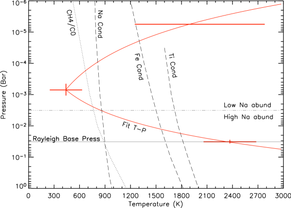
Figure 1: The parametric T–P profile of the atmosphere of HD 209458 b (thick red solid line), as adjusted over HST/STIS observations by Sing et al. (2008b). The three adjusted (T,P) parameters are shown with their temperature error bars (red). The tripled–dot–dashed line shows the level of Na abundance drop at 3 mbar pressure. The thin solid line shows the 32 mbar pressure measured at the base of the sodium absorption line using the Rayleigh scattering. The dotted line shows the CH₄/CO equilibrium curve. The dashed lines show the condensation curves for sodium, iron, and titanium.

The fit of the HD 209458 b absorption spectrum including profiles of sodium and Rayleigh scattering by H₂ yielded (Sing et al. 2008b) an estimate of the temperature–pressure (T–P) profiles for the atmosphere from $\sim$30 mbar to $\sim$10$\leavevmode\nobreak\ \mu$bar (see also Madhusudhan & Seager (2009) for related issues when retrieving temperature and abundances from transit data). This result has been obtained using a parametric profile to fit the data, assuming linear variations in temperature with altitude and two layers with constant slope of temperature versus altitude (Fig. 1). Nonetheless, with this method, two different profiles provide an equally good fit to the absorption spectrum: the first profile involves Na condensation to explain the abundance drop at the absorption depth of 1.485%; in the second profile the temperature is not low enough to allow the sodium condensation, and the decrease in sodium absorption at altitude above the plateau is interpreted by ionization. The two resulting T–P profiles are

1. In the first profile the temperature decreases down to less than 900 K, causing a sodium abundance drop by condensation at about 3 mbar (Fig. 1);

2. The second profile (not shown in Fig. 1) is nearly isothermal at about 2200 K, in which case the abundance drop is explained by partial ionization of atomic sodium above the 3 mbar level in a scenario proposed by Fortney et al. (2003).

Both profiles do not present variations similar to model predictions as calculated in the literature specifically for HD 209458 b. The direct comparison between extracted observational T–P profiles and model predictions will be made in Sect. 4 (Fig. 9).

To further reduce the impact of a priori hypothesis on the data interpretation, we propose here a new analysis of the absorption depth profile with particular attention to the inner part of the NaI doublet. This new analysis is done using a non–parametric approach, with no a priori assumption about any expected behaviour related to the T–P profile or to supposed NaI abundance variations. The hope is to be able to distinguish between the two scenarios described above, avoiding a priori assumptions. In Sect. 2 we present the method for the data analysis. In Sect. 3 we compare the observations to the model calculations. The results are discussed in Sect. 4 where a new description of the upper atmospheric layers of HD 209458 b is proposed.

2 The sodium absorption depth in the line core

Figure 2: The relative altitude of the absorption as observed by Sing et al. (2008a) close to the NaI lines in variable bandwidths (see text). Their photometric approach is presented as crosses with the corresponding error bars, while their spectroscopic approach is plotted as diamonds. The error bars corresponding to both evaluations are similar. These observations are correlated since extracted over variable bandwidths all centered on the NaI lines. Three main regions could be seen: [I] corresponding to a sharp decrease, [II] to a plateau and [III] to a more gentle decrease. Analysis of these three regions will be carried out starting from region [III] inward.

Sing et al. (2008a) evaluated the transit absorption depth around the center of the NaI lines in variable bandwidths from 4.4 to 100Å centered over both lines. At 12Å bandwidth, the measured absorption depth agrees with the Charbonneau et al. (2002) value. In the Sing et al. (2008a) approach, the absorption depth is evaluated relatively to a reference absorption depth in a fixed double spectral band (noted Ref) on both sides of the NaI lines: from 5818 to 5843Å and from 5943 to 5968Å, i.e. in a fixed 50Å region. The measurements are obtained by first integrating the raw data over the selected bandwidth before extraction of the absorption depth. Because the measurements correspond to the total absorption depths within various bands, including the line center as done with filters, this absorption spectrum as a function of the bandwidth can thus be regarded as a spectrum obtained with a “photometric” approach. The resulting “photometric” spectrum is plotted in Fig. 2.

In another approach, Sing et al. (2008a) also extracted spectroscopically the absorption depth distribution over each pixel in the whole spectral range covered by the observations. These spectroscopic absorption depths can also be averaged over different spectral bandwidths as in the photometric approach. We calculated the difference between the spectrum averaged over various bands centered on the NaI lines and the spectrum averaged in the reference band, Ref, defined above. The result obtained in this “spectroscopic” approach (see Figure 2) can be directly compared with “photometric” result. Small differences do show up between the two extraction methods, but they are well within the error bars. The main differences probably arise from the limb–darkening correction, which is applied at each pixel wavelength in the spectroscopic approach, while the correction is a weighted average limb–darkening correction in the considered bands in the “photometric” approach. Therefore, the “spectroscopic” is expected to provide a better correction for the limb–darkening variations within the stellar lines themselves and in particular within the two strong NaI doublet lines. In the following, we use the spectroscopic absorption depths.

In Figure 2 the measured absorption depths have been translated into planetary radii, i.e., altitudes above the Ref level, defined by the level of the absorption depth in the Ref spectral domain. To translate AD into altitudes above the Ref level, we used R_P=1.32R_Jup (Knutson et al. (2007)) for the planetary radius and an absorption depth of AD_Ref = 1.49145% at the Ref level. As expected, the observed altitudes (i.e. AD) vary as a function of the bandwidth with a slow rise toward smaller bandwidths; however, three different regions could be seen in terms of AD variations: a region [I] (see Fig. 2) presenting a rapid decrease of the AD with increasing bandwidths followed by a kind of plateau (region [II]), a puzzling feature discussed in Sect. 4 followed by a last region [III] where a slow decrease in the AD could be seen. These observations are not independent. In particular, the error bars are larger than the observations’ fluctuations. Indeed, all observations made in a given bandwidth are present in observation–extracted in any larger bandwidth. For that reason, we will complete our analysis of the observed behavior of the AD by starting from the larger bandwidths and moving inward. This approach will give us first access to the atmospheric information at the lower altitudes and then, by eliminating this information in the narrower bandwidths, move progressively upwards in the atmosphere.

3 Modeling the absorption spectrum

The variations in the absorption depth (or variations of the corresponding altitude) along the line profile are due to variations of the line opacity. At each wavelength, the absorption line probes different altitudes in the planetary atmosphere with a resolution on the order of the error bar on the absorption estimate, i.e. about 0.01% in absorption depth corresponding to about 315 km in altitude. Because the absorption cross section increases toward wavelengths closer to the core of the lines, the absorption depth increases toward narrower bandwidths (Fig. 2). These variations in absorption altitude (or absorption depth) can be interpreted through comparison with model calculations.

3.1 From absorption depth to physical quantities

To interpret the measured variations in absorption with bandwidths, we built the simplest possible model, i.e. an isothermal hydrostatic uniform abundance model (IHUA). The model with isothermal hydrostatic atmosphere at temperature $T$ with a single sodium abundance value ([Na/H], relative to the solar abundance), and a pressure $P_{z=0}$ at a reference level, is a three–parameter model ($T$,[Na/H],$P_{z=0}$). This model is aimed at a better understanding of the observed absorption depth variations in terms of departures from the local IHUA conditions, i.e. in terms of variations in temperature or sodium abundance, without any a priori hypothesis on the shape of the vertical temperature–pressure profile as needed in Sing et al. (2008a). Despite its simplicity, assuming hydrostatic equilibrium, this (IHUA) model still holds locally to interpret observational measurements because the atmospheric scale height is on the order of the observational accuracy, i.e. $\sim$ 300 km for typical temperatures in the HD 209458 b atmosphere. The exponential decrease in the volume density with altitude is very steep; as a result, the variations in the measured absorption at a given altitude are directly related to the physical conditions (temperature, abundance) in the atmosphere at the corresponding altitude.

The model absorption depth is calculated in a straightforward manner following Lecavelier Des Etangs et al. (2008a,b). The total column density along the line of sight passing through the terminator at different altitudes is given by Fortney et al. (2005). The optical depth, $\tau$, in a line of sight grazing the planetary limb at an altitude $z$ is given by

$$\tau(\lambda,z)\approx\sigma(\lambda)n(z)\sqrt{2\pi R_{P}H}$$ (1)

where $R_{P}$ is the planetary radius, $H$ the atmosphere scale height, and $n(z)=n_{(z=0)}exp(-z/H)$ the volume density at the altitude $z$ of the main absorbent with a cross section $\sigma(\lambda)$. The scale height is given by the relation $H=kT/\mu g$ where $k$ is the Boltzmann constant, $T$ the temperature, $\mu$ the mean mass of atmospheric particles taken to be 2.3 times the mass of the proton, and $g$ the gravity at the planetary radius, $g=M_{P}{\rm G}/R_{P}^{2}$ with $M_{P}$ equal to the planetary mass and G the gravitational constant. The absorption at a given wavelength, $\lambda$ is calculated by finding the altitude at which the optical thickness is $\tau(\lambda,z)=\tau_{eff}$, where $\tau_{eff}$=0.56 (Lecavelier des Etangs et al. 2008a ).

Using the equations and quantities defined above, the effective altitude $z$ is given by

$$z(\lambda)=H\ln\left(\frac{{\rm[Na/H]}\times P_{z=0}\times\sigma_{NaI}(\lambda)}{\tau_{eff}}\times\sqrt{2\pi R_{P}/kT\mu g}\right)$$ (2)

where $\sigma_{NaI}$ is the NaI lines cross section. Equation 2 shows that the altitude (or corresponding absorption depth) depends on pressure and abundance, but the variation in the altitude as a function of wavelength does not depend upon pressure or abundance, but only upon the scale height, which is directly and only related to $T$, the temperature at the corresponding altitude. Therefore, the interpretation of Fig. 2 (in particular the slope of the absorption depth curve as a function of wavelength) provides the temperature profile in the altitude range probed by the sodium line core: from 100 to 4 000 km altitude. This temperature profile can have a typical resolution close to the atmospheric scale height.

As shown by Eq. 2, the absolute values of the pressure and abundance impact only the absolute absorption altitudes and not their variations. Moreover, there is a degeneracy between these two quantities because only the product $[Na/H]\times P_{z=0}$ can be constrained by the measurement of the absorption altitude. In other words, a change in the abundance can be directly compensated by a similar change in the pressure. That is the total quantity of gas in the line of sight.

3.2 Pressure at the reference level

One could assume that the pressure at the reference level, $P_{z=0}$ for our NaI study in the core of the lines, i.e. as evaluated over the reference domain $Ref$ over which the AD_Ref evaluation is made and relative to which all our differential AD evaluations are made, is given by the H₂ Rayleigh scattering observed at wavelengths shorter than $\sim$5 000 Å (Lecavelier des Etangs et al. 2008b ). This leads to a reference pressure $P_{z=0}\sim$3 mbar as shown in Fig. 1. This pressure corresponds to the location where the NaI abundance drops and above which only the core of the NaI lines do give an absorption signature.

To be more precise, one could alternatively use the evaluated NaI abundance, $[Na/H]\sim 2$ found in the lower layers of the atmosphere by Sing et al. (2008a), to evaluate the corresponding pressure at the reference altitude. Indeed with only the product $[Na/H]\times P_{z=0}$ being defined, by using the evaluated NaI abundance in the lower layers one can deduce the pressure level sampled by the NaI lines at any spectral region. This is given by the following relation deduced from Eqs. 1 and 2.

$$P(\lambda)=\left(\frac{\tau_{eff}\times kT}{{\rm[Na/H]}\times\sigma_{NaI}(\lambda)\times\sqrt{2\pi R_{P}/kT\mu g}}\right).$$ (3)

Figure 3: The variation in the pressure as a function of wavelength is given according to Eq. 3 (solid line). Twice the solar NaI abundance is assumed. A temperature of 900K (corresponding to the sodium condensation temperature) is also assumed and the two spectral reference domains are indicated as vertical long dashed lines. In those regions the evaluated pressure (thick solid lines) is indeed on the order of 3 mbar as indicated by the horizontal dashed line.

The result of Eq. 3 is shown in Fig. 3 for which the assumed abundance is twice the solar abundance, valid up to our reference level. The pressure broadening in the NaI line wings is larger than the natural width broadening at pressures above 29 mbar as it could be scaled from the corresponding values at 1 bar and 2 000 K where the inverse lifetime related to pressure broadening is $\tau=0.071$cm${}^{-1}\times c=2.1\times 10^{9}$s^-1 to be compared to the natural inverse lifetime which is $6.1\times 10^{7}$s^-1 (Iro et al. (2005)). Because here we are analyzing the inner parts of the NaI lines (between the two reference domains, see Fig. 3), we only investigate the upper part of the atmosphere where lower pressures are present. We thus can ignore here the pressure broadening effects. Consequently, $\sigma_{NaI}(\lambda)$ in Eq. 3 was evaluated by taking only into account the Doppler core broadening and the natural wing broadening of both NaI doublet lines.

We find that, using a temperature of 900 K and sodium abundance twice solar, absorption over the two spectral reference domains, on both sides of the NaI lines from 5 818 to 5 843 Å and from 5 943 to 5 968 Å, is due to sodium located at a pressure of 3 mbar (Fig. 3).

If a different temperature is selected for the reference level (as for instance 2 000 K as suggested in the second possible scenario), then the evaluated pressure at the reference level would be slightly higher and on the order of 6 mbar, a value still within the pressure domain where the pressure broadening effect could be ignored. With this new reference pressure, the T–P profile obtained here would still hold with only a shift in the reference level from 3 to 6 mbar.

Once the reference pressure has been set, our IHUA model becomes a two–parameter model ($T$,[Na/H]) and the selection of a different reference pressure only slightly shifts our temperature evaluations along the pressure scale, with the sodium abundance modified by the same ratio.

Figure 4: Absorption depths calculated using IHUA models with $T$=500 K and $T$=1 000 K for various sodium abundances ranging from [Na/H]=10^-2, 10^-4, 10^-6, 10^-8, 10^-10 (top to bottom).

3.3 Temperature profile

In the framework of our study, we consider relative absorption depths, calculated by the difference in absorption depths between two spectral domains: the first one for a given bandwidth centered on the sodium lines, the second one in the constant Ref domain. If the [Na/H] abundance varies, the absolute absorption depth of all spectral domains changes by nearly the same amount (see Eq. 2). As a result, the relative absorption depth in the sodium line does not depend on the sodium abundance as shown in Figure 4. Indeed a change in the abundance produces about the same shift in the absorption depth at all wavelengths. Therefore, the difference between the absorption depth in a given bandwidth and the absorption depth in the reference wavelength domain (AD–AD_Ref) barely depends on the sodium abundance. On the contrary, the slope of the models clearly changes with temperature. The sodium abundance thus cannot be estimated by the transmission spectrum of relative absorption depth.

However, the variations in the relative absorption depth does allow estimating the local temperature $T$ at the absorption altitude. In effect, the variation in the absorption altitude with wavelength depends on the variation in the horizontal integrated density with altitude. For instance, if one considers two wavelengths $\lambda_{1}$ and $\lambda_{2}$, with corresponding line cross section $\sigma(\lambda_{1})>\sigma(\lambda_{2})$, a grazing line of sight will have the same optical thickness at these two wavelengths if they are at altitude $z_{1}$ at $\lambda_{1}$ and $z_{2}$ at $\lambda_{2}$ such that the variation in partial density of the absorbing element $n(z)$ between $z_{1}$ and $z_{2}$ compensates for the different cross sections. The optical thickness at these two wavelengths are equal if $n(z_{1})\sigma(\lambda_{1})=n(z_{2})\sigma(\lambda_{2})$. Therefore, the variation in the observed absorption altitude as a function of wavelength (equivalent to variation as a function of line cross section) reveals the variation in the partial density at the considered altitude. At hydrostatic equilibrium, the density variation with altitude is determined by the temperature through the characteristic scale height. As a consequence, the temperature constrains the slope of the absorption altitude as a function of wavelength. The higher the temperature, the larger the slope. For a given absorption feature with a known cross section as a function of wavelength, the temperature $T$ can be derived from the measurements of the absorption altitude spectrum using (Lecavelier des Etangs et al. 2008a ):

$$T=\frac{\mu g}{k}\left(\frac{d\ln\sigma}{d\lambda}\right)^{-1}\frac{dz(\lambda)}{d\lambda}.$$ (4)

Figure 5: Plot of the absorption altitude as a function of the wavelength band. Measurements of Sing et al. (2008a) are plotted: photometric with crosses and spectroscopic with diamonds. The typical error bars of all evaluations are shown only over the photometric evaluations to avoid confusion. The dashed line shows the best–adjusted IHUA (isothermal hydrostatic and uniform abundance) model to the lowest altitude observations, corresponding to a temperature of 340 K. For comparison the theoretical IHUA models are shown at $T=$ 140 K, 540 K (solid lines), shifted in ordinate toward the lower end of the first error bar at 105 Å in order to show the constraints on the model slopes (not affected by the applied shift) related to the observational error bars. This leads to an estimate of the temperature at the lower levels to be 340 $\pm$ 200 K. Similar errors on the order of $\pm$ 200 K are found for each observational region of about one scale height (see text). Finally, the 900 K model (dotted line) corresponding to the sodium condensation temperature (see Fig. 1) is also shown to illustrate its incompatibility with the observations.

Figure 5 shows the expected variations for fixed abundances of NaI over the whole atmosphere, overplotted with isothermal IHUA models at different temperatures. As explained above, the higher the temperature, the higher the scale height in the atmosphere and thus the steeper the slope. Here, the Na abundance corresponding to each temperature is assumed to be constant, while the model representations in Figure 5 are arbitrarily vertically shifted (thus keeping the same slope at each given wavelength) in order to match the observations above the reference level.

Figure 6: Same as in Figure 5 with IHUA models matching the observations up to 800 km in altitude. At the lowest altitude, the temperature is found to be $\sim$ 340 K (solid line). At altitude above $\sim$ 200 km, we identified layers with different temperatures at about 550 K (dashed line), 910 K (dotted line), then back to 550 K (dashed line). A few error bars are indicated to underline that, in the lower altitude region [III] from 0 to 800 km above the reference level, the observations are on the average incompatible with an IHUA model slope corresponding to $\sim$900 K, the sodium condensation temperature, demonstrating that condensation has to take place in the planetary atmosphere.

4 Results and discussion

4.1 The temperature profile at low altitudes (region [III])

Using the method described above, we start by evaluating the temperature at altitudes just above the reference level (altitude 0–225 km, bandwidths 75–110 Å), with the reference level corresponding to the level where the sodium abundance drops sharply ($\sim$3 mbar level). The temperature of the atmosphere just above the reference level (see Fig. 5) is found by the slope of the observed variations (see Eq. 4). In this atmospheric layer (region [III] as shown in Fig. 2), the absorption depth varies slowly as a function of the bandwidth. As a consequence, we find the lower temperature close to $\sim$ 340 K. Because this temperature appears to be extremely low, the assumption of uniform abundance is likely not to be valid for the scale height just above the reference level, a region probably still affected by the Na–depletion mechanism (see Sect. 4.4). From Eq. 2, the measured altitude is determined by the quantity of $[Na/H]\times\sigma_{NaI}(\lambda)$. If the Na abundance drops with increasing altitude, for a given optical depth through the atmosphere, the Na cross section needs to be larger to compensate, making the transmission spectrum optically thick closer to the Na core. As a result, a depletion in sodium causes a shallower slope (or even a plateau) in the observed absorption depth versus bandwidth. In other words, if the temperature is measured by the slope of the absorption altitude as a function of wavelength assuming a constant abundance, a decrease in sodium abundance with altitude implies underestimation of the temperature (Eq. 4). The temperature of 340 K is therefore a lower limit of the temperature in the layer located in the altitude range from 0 to 200 km above the reference level. In this layer, the temperature is likely higher and the abundance of sodium is very likely decreasing with altitude.

Apart from the shallow slope of absorption as a function of the bandwidth described above, we observe two sodium absorption–depth plateaus at 80 Å and 55 Å bandwidth. This can also be interpreted as abundance drops at the corresponding altitudes. We however ignore these two plateau regions because they are entirely immersed within the error bars domain (see Fig. 5). We thus assume locally constant abundance (at least over one scale height) to estimate the local temperature in the different layers of the atmosphere.

Figure 7: Same as Figure 6 for narrower bandpass, i.e. corresponding to regions [I] and [II] at higher altitudes from 800 km to 4 000 km.

The temperature profile can thus be obtained step by step toward increasing altitude by analyzing the observed AD variations in narrower bandpasses. When starting from wavelength bandwidths of 110 Å, working toward shorter bandwidths, and assuming constant abundance, the AD variations can be interpreted in terms of temperature changes as a function of altitude with the following characteristics (see Fig. 6):
i) a lower limit of 340 K in temperature is obtained at the lowest altitudes,
ii) between altitudes of 200 km and 400 km, the temperature is found to be about 550 K,
iii) the AD slope constraints the temperature at about 910 K in the layer between 400 km and 600 km altitude,
iv) the temperature seems to drop back close to 550 K between 600 km and 800 km altitude.
For each layer considered, the error bars on these temperature evaluations are of about $\pm 200$ K, similar to the error estimate made on the lowest temperature level at 340 K as shown in Fig. 5. Therefore, the observed temperature variations correspond to a marginal rise in temperature with altitude.

Most importantly, for about three scale heights from 200 to 800 km above the altitude where the NaI abundance is seen to drop sharply, the atmospheric temperatures are found to be within the range $\sim$ 550 – 910 K, i.e. below the sodium condensation temperature (Figure 1). This result favors the sodium condensation scenario to explain the sodium abundance drop as described in (Sing et al. 2008a ; Sing et al. 2008b ). Recent global climate models of HD 209458 b also suggest cool temperatures of $\sim$ 800 K (at mbar pressures) are possible on the night–side of the planet and terminator (Showman et al. (2009)), further supporting this sodium condensation model.

Figure 8: Same as in Figure 6 for the narrowest bandpass (region [I]). Near to the line center, the cross section is the highest, therefore probing the highest altitudes. The ground–based measurements obtained by Snellen et al. (2008) are plotted with crossed squares together with the spectroscopic evaluations (diamonds) of Sing et al. (2008a). The variations of the absorption depth (AD) between 1.5 and 3Å bandpass are consistent with a temperature from 1 500 to 4 000 K with the most plausible value on the order of 2 500 K.

Figure 9: Plot of the “integrated–averaged” T–P profile (diamonds) obtained in Sect. 4.3. The vertical error bars show the pressure domain of the corresponding temperature estimates. The triple–dot–dashed line shows the altitude of the sodium abundance drop measured by (Sing et al. 2008a ; Sing et al. 2008b ). At pressure between $10^{-3}$ and $10^{-5}$ bar, the low temperature ($T<800$K) favors the sodium condensation scenario to explain the sodium abundance drop. Our T–P profile is consistent with the T–P profile obtained by Sing et al. (2008b) using a parametric fit of the same data set (dotted line) without the addition of the latest observations at higher altitude levels from Snellen et al. (2008). For comparison several theoretical T–P profiles are over plotted. At higher pressures (P$>$1 mbar), models of Barman et al. (2005; dash–triple–dotted line), Showman et al. (2008; long dashed line) and Guillot (2010; two solid lines, one for $\mu=0$ at the terminator limb and the other at $\mu=0.1$ close to the terminator limb) are shown. At lower pressure levels, the Yelle (2004) theoretical T–P profile is also shown for comparison (dashed line). The dot–dashed line shows the vertical velocity of the hydrodynamic outflow in the Yelle (2004) model (in m/s). This velocity is negligible at pressure above a few $10^{-8}$ bar where the hydrostatic assumption is therefore justified.

4.2 The temperature profile at higher altitudes(regions [I] and [II])

The temperature at higher altitudes can be estimated by looking for the AD variations over narrowest bandpasses. There, an important and significant leveling off (region [II]) of the AD variation at about 800 km altitude, between 32Å and 20Å bandwidths, is seen (note in Fig. 7 its position relative to the observational error bars). This plateau in absorption depth might be interpreted as a local drop in temperature but this would correspond to an extremely low temperature of less than 100 K ! This plateau is more likely related to a decrease in sodium abundance which will be further discussed in Sect. 4.4.

Above that long leveling off, i.e. above 800 km altitude (region [I]), the AD increases again rapidly toward shorter bandwidths (from 15Å bandpass and below), revealing there a rise in temperature. Using an IHUA model fit to the AD profile, we find a typical temperature of about 1500 K from about 800 km up to 4 000 km altitude (Fig. 7). The measurement at 4 000 km corresponds to the narrowest 3Å bandpass in the very center core of the line in HST observations. It is noteworthy that this 1 500 K atmospheric layer is observed to be isothermal over nearly 6 scale heights. Over this wide altitude range, the error bar on the estimated temperature is rather small ($\pm$100 K). There the temperature is tightly constrained in the 1 400 K–1 600 K range.

After publication of the HST data analysis by Sing et al. (2008a), new measurements of the Na i absorption depth have been obtained by Snellen et al. (2008) using ground–based observations. These measurements have been obtained in narrower bandpasses, providing larger absorption signatures, therefore corresponding to absorptions at higher altitudes. These new measurements are shown in Fig. 8 together with those of Sing et al. (2008a). Although these various measurements have been obtained using very different techniques, and despite that ground–based measurements are known to be extremely difficult because of the Earth atmospheric perturbation, the very good agreement between the various data sets strengthens the confidence in those measurements permitting us to extend our analysis in altitude up to more than 6 500 km.

On the contrary, we decided not to use the recent ground–based observations of Langland–Shula et al. (2009) because their result suffers from uncertainties in the process of continuum fitting and subtraction of the Earth atmosphere absorption.

We find that to match the variations of the absorption depth toward the narrowest 1.5 Å bandwidth as measured by Snellen et al. (2008) , the temperature at altitudes above 4 000 km needs to be on the order of 2 500 K and within a 1 500 – 4 000 K range (Fig. 8).

4.3 The “integrated–averaged” T–P profile

An important comment here before presenting the result is to recall that the evaluated T–P profile is extracted from quantities “integrated” along the cords passing through portions of the limb presenting gradients, e.g. from the night to day sides, as well as “averaged” over the planetary limb, e.g. from equatorial to polar regions. In a first step, such an “integrated–averaged” T–P profile could be compared to 1–D model calculations, although it is clear that later steps, when observations permit it, would be to compare them to more sophisticated 3–D models as illustrated in e.g. the Iro et al. (2005) and the recent Fortney et al. (2010) studies.

From the temperature–altitude relation obtained in Sects. 4.1 and 4.2, and assuming hydrostatic equilibrium, we can calculate the temperature–pressure (T–P) profile. We start by using a reference pressure of 3 mbar at the reference 0 km altitude. The pressure is calculated step by step, starting from the zero altitude level. The result is shown in Fig. 9.

Acknowledging that the sodium condensation occurs at temperatures below 800 – 900 K, the temperatures measured in the layer between 0 and 800 km above the reference level are found to be low enough to allow condensation. This condensation seems to take place at pressures between 3 mbar and 10 $\mu$bar.

As already mentioned in the introduction, at pressures above 3 mbar, the evaluated observational profiles do not present variations similar to the model predictions as calculated in the literature specifically for HD 209458 b (e.g. Barman et al. 2002; Burrows et al. 2003; Iro et al. 2005; Barman et al. 2005; Fortney et al. 2008; Showman et al. 2008; Showman et al. 2009; Guillot 2010; Fortney et al. 2010). Three of them (Barman et al. 2005; Showman et al. 2008; Guillot 2010) are presented in the lower part of Fig. 9. It is interesting to note that all temperature predictions at about 3 mbar are in good agreement with our evaluation simply made from the direct estimation of the scale height at these levels. We also point out the large variations revealed by the two near terminator–limb (i.e. near the transit observed limb) model calculations from Guillot (2010; one for $\mu=0$ at the terminator limb and the other at $\mu=0.1$ close to the terminator limb) as also shown in Fig. 9. This may indicate that indeed such model predictions are difficult to compare to observations according to their extreme sensitivity to the precise limb geometry and, as already said, to the integrated nature of the observations along a grazing line of sight. Also, one could argue that at higher pressures, it is not surprising that observations (and their interpretation) differ from theoretical models, since for instance, a large heat advection could be critical in the troposphere leading to strong departures from equilibrium temperature profiles.

Above this condensation layer, a progressive rise in the temperature with altitude is needed to explain the profile of the sodium line toward narrower bandpasses. The temperature in the upper atmosphere is found to reach $\sim$ 2 500 K at the very low pressures of $\sim$ 3 to $\sim$ 90 nbar. This is likely the signature of the base of the thermosphere, which is the expected transition between the cool lower atmosphere and the hot upper atmosphere where hydrodynamic atmospheric escape takes place. This scenario agrees with theoretical models of the atmospheric escape as published by, e.g., Lecavelier des Etangs et al. (2004), Yelle (2004) overplotted in Fig. 9, Tian et al. (2005), Yelle (2006), Muñoz (2007), and Murray-Clay et al. (2009).

A summary of our T–P profile is given in Table 1. The scale heights $H$ are given for each temperature layer. This shows that the layers have thicknesses of at least one or more scale heights. With a pressure change by a factor of 2.7 over one scale height under hydrostatic equilibrium, Fig. 9 shows that the bottom layer at the lowest temperature of $>$ 340 K has a thickness of nearly 2 scale heights. The three following layers at 550 K and 910 K are over about 1 scale height, while the atmospheric layer with a constant temperature at $\sim$ 1 500 K extends over nearly 6 scale heights. Finally the last upper layer at about 2 500 K extends over more than 3 scale heights.

The calculated T–P profile is valid when assuming local hydrostatic equilibrium. This assumption could be invalid because of the hydrodynamical escape of the upper atmosphere. Figure 9 shows that the theoretical escape velocities triggered by the hydrodynamic flow as evaluated by Yelle (2004) are negligible below the altitude corresponding to a pressure of $\sim$ 10^-9 bar. This shows that the local hydrostatic equilibrium assumption is valid over our studied range, even at the highest altitudes where we estimate a temperature of about 2 500 K.

Table 1: Evaluated atmospheric parameters

$z$ min	$z$ max	$T\pm\Delta T$	$H$	$H/\Delta z$	$P_{\rm max}$	$P_{\rm min}$
(km)	(km)	(K)	(km)		(bar)	(bar)
0	225	340${}^{+200}_{\leavevmode\nobreak\ -\leavevmode\nobreak\ 0}$	120	1.9	3.0e-3	5.0e-4
170	390	550$\pm$200	200	1.1	5.0e-4	1.7e-4
350	620	910$\pm$200	340	0.8	1.7e-4	7.7e-5
620	800	550$\pm$200	200	0.9	7.7e-5	3.1e-5
800	4 000	1 500$\pm$100	540	5.9	3.1e-5	9.4e-8
3 500	6 500	2 500${}^{+1\,500}_{-1\,000}$	920	3.3	9.4e-8	3.6e-9

4.4 The Na abundance profile

The sodium abundance [Na/H] cannot be constrained in absolute terms according to the mentioned degeneracy between abundance and pressure in the absorption spectrum (see Lecavelier Des Etangs et al. 2008a and Eq. 2). However, here the degeneracy can be solved by assuming a reference pressure at the reference level (see Section 3.2). Indeed we used a reference pressure of 3 mbar for the altitude corresponding to our reference level at 1.49145% absorption depth. Using in addition the sodium abundance below the reference level as evaluated by Sing et al. (2008b) in the lower layers of the atmosphere, [Na/H]$\sim$3$\times$10^-6 (solar abundance equals 1.5$\times$10^-6, Asplund et al. 2006), we can deduce the sodium abundance evolution in the upper layers. In agreement with the condensation scenario, the sodium abundance drops just above the reference level and then, following the upward evaluation of Sing et al. (2008b), it should be reduced on the average over all the upper layers by about a factor 10.

Starting from the value at the reference level, the Na abundance is evaluated at higher levels using a step–by–step procedure with local IHUA models. A constant [Na/H] abundance in the isothermal layers obtained in Sects. 4.1 and 4.2, has to be present, in agreement with our IHUA hypothesis.

A plateau in the measured absorption depth is observed at an altitude of about 800 km. This plateau is a kind of anomaly: with the increase of absorption cross section in the core of the line, the AD should rise toward smaller bandwidths. If the plateau was extending to the smallest bandwidths at the center of the line, this would reveal the absence of the absorber at altitudes above this plateau. However, here the plateau has a limited extension from $\Delta\lambda_{1}\sim 15$ Å to $\Delta\lambda_{2}\sim 30$ Å bandwidth. The absorption depth rises clearly again at bandwidths smaller than about 15 Å (see Fig. 7). This reveals a drop in the sodium abundance at the altitude of the plateau, but the sodium is still present above, thereby producing the observed absorption rise toward the line center. Along the plateau, the variation on the line cross section with wavelength, from $\sigma(\lambda_{1})$ to $\sigma(\lambda_{2})$, is compensated for by the variation in the sodium abundance, ${\rm[Na/H]}_{1}$ and ${\rm[Na/H]}_{2}$ above and below the plateau altitude. Using Eq. 2, the altitude of the plateau $z(\lambda)$ being constant from $\lambda_{1}$ to $\lambda_{2}$, we find that

$$\left(\frac{{\rm[Na/H]}_{1}}{{\rm[Na/H]}_{2}}\right)=\left(\frac{\sigma(\lambda_{2})}{\sigma(\lambda_{1})}\right).$$ (5)

Because here the absorption is dominated by the damping wings of the sodium line, we have

$$\left(\frac{\sigma(\lambda_{2})}{\sigma(\lambda_{1})}\right)\cong\left(\frac{\lambda_{2}-\lambda_{0}}{\lambda_{1}-\lambda_{0}}\right)^{-2}.$$ (6)

With $\Delta\lambda_{2}/\Delta\lambda_{1}\sim$2  for the plateau at 800 km of altitude, we can determine that this plateau may be explained by a drop in sodium abundance by a factor [Na/H]₂/[Na/H]₁ $\sim$ 4. According to our approach, which is essentially local, we can conclude about this relative local drop, while as stated earlier, absolute values of the sodium abundances could not be assessed. To represent these absolute values, we used the result of the global approach of Sing et al. (2008a,b) as shown in Fig. 10.

Figure 10: Summary of the Na abundance estimates using the IHUA model. Because our approach is local we can only identify here the decreases in sodium abundance by a factor of about 4 at $3\times 10^{-5}$ bar (dot-dashed line), although NLTE effects could perturb that estimation (see text). The drop in abundance by about a factor of 10 showed at the condensation level (at 3 mbar, tripled–dot–dashed line) is taken from Sing et al. (2008a,b).

Considering the sodium abundance drop evaluated by Sing et al. (2008a,b) at the condensation level to be on the order of a factor of 10, we assumed that [Na/H]₂ should be on the order of 0.2 solar, while the Na abundance above the altitude of the plateau should be [Na/H]₁$\sim 0.05$ solar. Figure 10 shows the Na abundance variations obtained from the observed AD over the whole domain sampled in Fig. 9.

To match the observed AD plateau, one has to assume a local reduction in the Na abundance by a factor of about 4, which could indicate of a possible physical effect in the atmosphere, such as the ionization of NaI into NaII as predicted by several models, e.g. Fortney et al. (2003). The conclusion on the drop in the Na abundance to interpret the AD plateau is expressed in terms of relative abundance, so this conclusion does not depend upon any assumption about pressure or absolute abundances.

We are evaluating variations in the Na abundance in low volume density regions where nonlocal thermodynamic effects (NLTE) should take place, i.e. below 1 mbar as evaluated by Barman et al. (2002). There radiative processes dominate collisional ones and the NaI population levels could be significantly away from the assumed local thermodynamic equilibrium (LTE) ones. As long as such effects do not vary significantly over one scale height, our temperature evaluations should not be affected by these NLTE effects. On the contrary, such effects certainly should perturb abundance evaluations, and in particular, the previously mentioned factor 4 drop of abundance at $3\times 10^{-5}$ bar could as well be the signature of such NLTE effects at these altitudes, leading probably to an underestimation of the evaluated drop (Barman et al. 2002). If the corresponding signature is indeed due to Na ionization, it is in reasonably good agreement with the Barman et al. (2002) evaluation who found that Na would be mostly ionized in the limb for P $<$ 10^-6 bar and only partially ionized ($\sim$ 3%) below this point.

5 Conclusion

Using the measured NaI absorption depth as a function of the bandwidths, we estimated temperature variations as a function of altitude. Our temperature profile is inconsistent with one of the two scenarios of Sing et al. (2008b) (scenario with constant temperature and ionization at low altitude).

We found layers at temperatures clearly below the NaI condensation temperature showing that sodium condensation has to take place at these levels, followed by a temperature rise at higher altitudes up to about 2 500 K. This rise is likely the signature of the thermosphere needed to link the cool lower to the hot upper atmosphere, as suggested by the observations of atmospheric escape (Vidal–Madjar et al. (2003, 2004); Linsky et al. (2010)), observations of high temperatures (Ballester et al. (2007)), and models of the escape mechanism (Lecavelier des Etangs et al. (2004); Yelle (2004); Tian et al. (2005); Yelle (2006); Muñoz (2007); Murray–Clay et al. (2009)).

The results of our analysis favor the sodium condensation scenario to explain the deficiency of sodium observed in the line core, and the possible presence of an Na ionization layer just below the base of the thermosphere. Our temperature profile presents the following patterns:

– a rise from 340 K to 1 500 K over $\sim$800 km (about 5 scale heights) in the pressure range of $3\times 10^{-3}$–$3\times 10^{-5}$ bar;

– a thick layer with a nearly constant temperature at about 1 500 K. This layer has a thickness of about 3 200 km corresponding to nearly 6 scale heights for a pressure range of $3\times 10^{-5}$–10^-7 bar;

– a further temperature rise is observed at higher altitudes, up to 2 500 K at the highest altitudes about 6 500 km above the reference level, corresponding to a pressure of about $3\times 10^{-9}$ bar. This high temperature is likely related to the bottom part of thermosphere whose presence is predicted by theoretical models of the atmosphere.

– an NaI abundance drop by a factor of 4. This is possibly due to ionization at the $3\times 10^{-5}$ bar level, the strength of the observed drop depending upon the importance of the NLTE effects at these altitudes.