The possible bound state of the double heavy meson-baryon system

Abstract

We calculate the two-pion exchange potential between a heavy meson and a heavy baryon. We find this potential is as strong as the one-pion exchange potential between two heavy mesons and is enough to bind $\Lambda_{b}-\bar{B}$. Though our result is sensitive to the cut-off, the value of the cut-off is in the reasonable region.

1 Introduction

In the naive quark model, there are no more than three quarks and anti-quarks in a hadron. This picture is not quite consistent with the fundamental theory of the strong interaction, Quantum Chromodynamics (QCD), because colour singlets can be formed from larger numbers of quark constituents. Thus it is generally believed that hadron configurations should exist beyond the naive quark model, i.e., hadrons composed of four, five or more quarks and anti-quarks. Actually, the nuclei, which can be considered as multi-quark states, have already been found long ago. It is amazing that the four and five quark states have not been found yet. It is possible that QCD dynamics prevents the formation of these states or their experimental observation may be difficult. For QCD itself, the confirmation of such “exotic” hadrons in experiments surely is welcome .

The simplest extension of the naive quark model is the four-quark state [1]. Some four-quark states may have “exotic” quantum numbers and can be easily distinguished from the “normal” mesons, but because most of them have the same quantum number as the “normal” mesons, identification of them becomes challenging. At present, there is a focus on the so-called molecule states, which have an anomalously large decay width in a special channel in which the masses of the states are on the kinematic threshold. The famous examples are $f_{0}(980)$ and $X(3872)$. Such molecule states are considered as loose bound states of two normal mesons via pion exchange [20]. This picture is very similar to the nuclei.

For the five-quark state [2], the train of thought is similar. Some states [e.g., the candidate $\theta(1540)$] do not mix with the normal baryons and can be identified easily. But most of them [e.g., the candidate $N^{*}(1535)$)] may be confused with the normal baryons. The configuration of the five quark states has two types, the diquark correlation and the meson-baryon bound state system. The $N^{*}(1535)$ is often considered as the bound state of $K\Sigma$ [14]. However, most discussions on meson-baryon molecules is restricted to light meson-baryon systems. This could be attributed to either experimental difficulties or challenging dynamics. In the meson-meson system, the one-pion exchange plays the most important role in binding two mesons. In the meson-baryon system, since there is no one-pion exchange (OPE), the four-particle interaction, such as the $\bar{N}N\bar{K}K$ interaction in the case of the $\Lambda(1405)$ (which is considered as a quasi-bound state of $\bar{K}N$ [26]), is very important. The coupling of the four-particle interaction can be fixed within Chiral Perturbation Theory (CPT) only if the constituent meson of the system is a goldstone boson. For the double heavy meson-baryon system, such as the $\Lambda_{c}\bar{D}$ system which we will consider, the four-particle interaction is currently unknown and its simple extension may have a large uncertainty. Instead, we consider two-pion exchange (TPE) in the $\Lambda_{c}\bar{D}$ system.

TPE not only can provide intermediate and long distance interactions, but also can provide the short distance interaction. The magnitude of TPE may be referred to the nucleon’s case. In nuclei, TPE is important partly because of the large coupling $g_{N\Delta\pi}$ [8] [9]. For our case, the coupling between heavy baryons is also very large [17]. As a naive dimensional analysis [7], the ratio between TPE of $D\Lambda_{c}$ and OPE of $D\bar{D}^{*}$ is $g_{4}^{2}M_{\sigma}\mu/(8\pi f_{\pi}^{2})$ (we use OPE for $D\bar{D}^{*}$ because there is no OPE between $\Lambda_{c}D$). The energy scale $\mu^{2}v=(M_{\Sigma}-M_{\Lambda})^{2}-M_{\pi}^{2}\approx(200MeV)^{2}$, $g_{4}\approx=1.24\pm 0.17$, so $D\bar{D}^{*}$ is $g_{4}^{2}M_{\sigma}\mu/(8\pi f_{\pi}^{2})\sim 1$. For $D\bar{D}^{*}$, many authors claim [10][19][20][13] that OPE may be strong enough to bind $D\bar{D}^{*}$ together. So it is appropriate to consider effects of TPE between $D\Lambda_{c}$. Without any information about counter terms (the four-particle interaction), our calculation is clearly dependent on the cutoff. A reasonable cutoff may be chosen by referring to the deuteron and X(3872) cases.

From the experimental point, SELX has already claimed the existence of the double heavy baryon $\Xi_{cc}$ [15]. Along with more and more double heavy baryons being found in experiments, the situation may become very similar to heavy quarkonium, i.e., many resonances may be considered as molecule states, such as X(3872), $Z_{b}(10608)$ [5]. Even the double heavy baryon-baryon state has been already considered [6]. The possibility of the double heavy meson-baryon state will be considered eventually.

In this paper, we consider the bound state of the $\bar{D}(\bar{B})-\Lambda_{c}(\Lambda_{b})$ system via TPE between the $\bar{D}(\bar{B})$ and the $\Lambda_{c}(\Lambda_{b})$. The two-pion exchange potential (TPEP) is regularized by a Gaussian type form factor [22] [24]. The potential is sensitive to the cut-off $\Lambda$ as expected, but we find it is as strong as the one-pion exchange potential (OPEP) of the $\bar{D}-D^{*}$ and $\bar{B}-B^{*}$ system at $\Lambda\sim 1GeV$, and the latter is believed strong enough to bind the two heavy mesons. Then we discuss the bound state of of the $\bar{D}(\bar{B})-\Lambda_{c}(\Lambda_{b})$ system by solving the Sch$\ddot{o}$dinger equation and find a bound state for $\Lambda\sim 1GeV$. Finally, we give a brief discussion and conclusion.

2 Two-pion exchange potential and the bound state of $\bar{D}-\Lambda_{c}$

The effective chiral lagrangian for the heavy mesons and baryons were already given in [16] [17]. For the heavy meson system, the lagrangian can be systematically expanded in the powers of small external momenta

$$\mathcal{L}=-i\text{Tr}\overline{H}_{a}\nu_{\mu}\partial^{\mu}H_{a}+\frac{1}{2}i\text{Tr}\overline{H}_{a}H_{b}\nu^{\mu}(\xi^{\dagger}\partial_{\mu}\xi+\xi\partial\xi^{\dagger})_{ba}+\frac{1}{2}ig\text{Tr}\overline{H}_{a}H_{b}\gamma_{\nu}\gamma_{5}(\xi^{\dagger}\partial_{\mu}\xi-\xi\partial\xi^{\dagger})_{ba}+\cdots$$ (1)

with

$$H_{a}=\frac{1+\not{\nu}}{2}(P_{a\mu}^{*}\gamma^{\mu}-P_{a}\gamma_{5})$$

$$\overline{H}_{a}=(P_{a\mu}^{*\dagger}\gamma^{\mu}+P_{a}^{\dagger}\gamma_{5})\frac{1+\not{\nu}}{2},$$

where

$$M=\left[\begin{array}[]{ccc}\frac{\pi^{0}}{\sqrt{2}}+\frac{\eta}{\sqrt{6}}&\pi^{+}&K^{+}\\ \pi^{-}&-\frac{\pi^{0}}{\sqrt{2}}+\frac{\eta}{\sqrt{6}}&K^{0}\\ K^{-}&\overline{K^{0}}&-\sqrt{\frac{2}{3}}\eta\end{array}\right],$$

$\Sigma=e^{2iM/f_{\pi}}$ with $f_{\pi}=132\,MeV$ and $\xi=\Sigma^{1/2}$. $\nu_{\mu}$ is the velocity of the heavy meson, $g$ is the coupling constant and

$$V_{\mu}=\frac{1}{2}(\xi^{\dagger}\partial_{\mu}\xi+\xi\partial_{\mu}\xi^{\dagger}),$$

$$A_{\mu}=\frac{i}{2}(\xi^{\dagger}\partial_{\mu}\xi-\xi\partial_{\mu}\xi^{\dagger}).$$

In this paper, we only consider the leading order of the heavy meson expansion and the order of the chiral expansion up to $O(p^{2}/(4\pi f_{\pi})^{2})$, so after substituting D meson fields for $P$ and $P^{*}$, we can write the interaction part of Eq.(1) in the rest reference frame of the heavy hadron (which is also approximately the center of mass reference frame of system we will discuss) as

$$\mathcal{L}_{DD*} = \frac{-2}{f_{\pi}^{2}}\overline{D}t\cdot(\pi\times\dot{\pi})D-\frac{2g}{f_{\pi}}(\sqrt{2}D^{*\dagger}t\cdot\vec{\nabla}\pi D+\sqrt{2}D^{\dagger}D^{*}t\cdot\vec{\nabla}\pi)-\frac{2}{f_{\pi}^{2}}\overline{D}^{*}t\cdot(\pi\times\dot{\pi})D^{*},$$

where $2t$ is Pauli matrix.

For the heavy baryon, the lagrangian is written as [17]

$$\begin{array}[]{lll}\mathcal{L}&=&\frac{1}{2}\text{Tr}[\overline{B}_{\overline{3}}(i\not{D}-M_{\overline{3}})B_{\overline{3}}]+\text{Tr}[\overline{B}_{6}(i\not{D}-M_{6})B_{6}]\\ &&+\text{Tr}\{\overline{B}_{6}^{*\mu}[-g_{\mu\nu}(i\not{D}-M_{6}^{*})+i(\gamma_{\mu}D_{\nu}+\gamma_{\nu}D_{\mu})-\gamma_{\mu}(i\not{D}+M_{6}^{*})\gamma_{\nu}]B_{6}^{*\nu}\}\\ &&+g_{1}\text{Tr}(\overline{B}_{6}\gamma_{\mu}\gamma_{5}A^{\mu}B_{6})+g_{2}\text{Tr}(\overline{B}_{6}\gamma_{\mu}\gamma_{5}A^{\mu}B_{\overline{3}})+H.C.+g_{3}\text{Tr}(\overline{B}_{6\mu}^{*}A^{\mu}B_{6})+H.C.\\ &&+g_{4}\text{Tr}(\overline{B}_{6}^{*\mu}A_{\mu}B_{\overline{3}})+H.C.+g_{5}\text{Tr}(\overline{B}_{6}^{*\nu}\gamma_{\mu}\gamma_{5}A^{\mu}B_{6\nu}^{*})+g_{6}\text{Tr}(\overline{B}_{\overline{3}}\gamma_{\mu}\gamma_{5}A^{\mu}B_{\overline{3}}),\end{array}$$ (2)

where $g_{i},i=1,6$ are coupling constants, $B_{3}$, $B_{6}$ and $B^{*}_{6}$ are the fields of anti-triplet , sextet baryons with 1/2 spin and sextet baryons with 3/2 spin respectively. Explicitly,

$$B_{6}=\left[\begin{array}[]{ccc}\Sigma_{Q}^{+}&\frac{1}{\sqrt{2}}\Sigma_{Q}^{0}&\frac{1}{\sqrt{2}}\Xi_{Q}^{{}^{\prime}+1/2}\\ \frac{1}{\sqrt{2}}\Sigma_{Q}^{0}&\Sigma_{Q}^{-}&\frac{1}{\sqrt{2}}\Xi_{Q}^{{}^{\prime}-1/2}\\ \frac{1}{\sqrt{2}}\Xi_{Q}^{{}^{\prime}+1/2}&\frac{1}{\sqrt{2}}\Xi_{Q}^{{}^{\prime}-1/2}&\Omega_{Q}\end{array}\right],$$

$$B_{\overline{3}}=\left[\begin{array}[]{ccc}0&\Lambda_{Q}&\Xi_{Q}^{+1/2}\\ -\Lambda_{Q}&0&\Xi_{Q}^{-1/2}\\ -\Xi_{Q}^{+1/2}&-\Xi_{Q}^{-1/2}&0\end{array}\right],$$

$B^{*}_{6}$ is similar to $B_{6}$. $M_{3}$ , $M_{6}$ and $M^{*}_{6}$ are the masses of anti-triplet , sextet baryons with 1/2 spin and sextet baryons with 3/2 spin respectively. Similarly, keeping the leading order of the chiral expansion, we obtain the interaction part of Eq.(2)

$$\mathcal{L}=\frac{-g_{2}}{f_{\pi}}\Sigma_{c}\gamma_{\mu}\gamma_{5}\partial^{\mu}\pi\Lambda_{c}+H.C.+\frac{-g_{4}}{f_{\pi}}\Sigma_{c}^{*}\partial^{\mu}\pi\Lambda_{c}+H.C.+\frac{-1}{f_{\pi}^{2}}\Lambda_{c}t\cdot(\pi\times\dot{\pi})\Lambda_{c}.$$

Normally, the coupling constants $g$ and $g_{i}(i=1,6)$ should be determined by the experimental data. From the decay width $\Gamma(D^{*}\to D\pi)$ [18], one can obtain $g=0.59\pm 0.06$. (In the following, we only use the central value $g=0.59$. This value is widely used, for instance see [7].) In the absence of the experimental data, $g_{i}(i=1,6)$ could be determined by the heavy quark symmetry and quark model [17]. From [17], $g_{4}=-\sqrt{3}g_{2}$, $g_{4}=1.24\pm 0.17$. $g_{1}$, $g_{3}$, $g_{5}$ and $g_{6}$ are not needed in this paper.

Since $\Lambda_{c}$ is an isospin singlet, there is no $\Lambda_{c}\bar{\Lambda}_{c}\pi$ interaction, but there is a $\Sigma_{c}\bar{\Sigma}_{c}\pi$ interaction. However, because the coupling $g_{1}$ in Eq.(2) is much smaller than $g_{2}$ and $g_{4}$ [17], the interaction $\Lambda_{c}\bar{\Sigma}_{c}\pi$ is more important. In the $\bar{D}-\Lambda_{c}$ system, $\pi^{\pm},\pi^{0}$ can be exchanged via the intermediate state $\Sigma_{c}$, while there is only one sort of pion that can be exchanged in the $\bar{D}-\Sigma_{c}$ via the intermediate state $\Lambda_{c}$. Therefore, we only consider the $\bar{D}-\Lambda_{c}$ system in the following.

The calculation of the two-pion exchange potential is quite straightforward. The divergence can be regularized by introducing a gaussian cut-off [22] [24] or in the dimensional regularization scheme [23]. Although the scheme of dimensional regularization seems more elegant, it is not suitable for our case. In the dimensional regularization scheme, the potential behavior at short distance is $1/r^{5}$ or $1/r^{6}$ (which has a singularity at r=0) [23], the origin of this behavior is the divergent momentum integral in the Fourier-transformation to coordinate space. Thus a cutoff is needed to regularize the short distance behavior; In the absence of any information about counter terms (short distance interaction), this scheme is also sensitive to the cut-off. The cut-off scheme is widely used for phenomenological estimates. The shortcoming of this scheme is sensitivity to cut-off dependence. The dependence on the cut-off should be removed by counter terms for which we have no knowledge. But we still can get useful information if we choose a suitable cut-off. For example, a cutoff of the order of the breakdown scale can serve as an order-of-magnitude estimate for unknown counter terms.

The calculation is very similar to that for the nucleon-nucleon potential [22] [24], except that the parallel box diagram in our case is a little bit different. In the nucleon case, one should be careful to extract the “iterated one-pion exchange” contribution [23]. Therefore, “old-fashioned” time-ordered perturbation theory is widely used [22]. However, there is no one-pion exchange between $D$ and $\Lambda_{c}$, so we can calculate directly using covariant perturbation theory.

Mass differences, such as $a=2(M_{D^{*}}-M_{D}$) and $b=2(M_{\Sigma_{c}}-M_{\Lambda_{c}})$, play important roles in our calculation, so we keep them in the heavy hadron mass expansion. For instance , we write the propagator of the $D^{*}$ meson as

$$T_{D^{*}}=-\frac{M_{D^{*}}g_{\mu\nu}}{(p_{1}-\frac{l-q}{2})^{2}-M_{D^{*}}^{2}+i\epsilon}=-\frac{g_{\mu\nu}}{-l_{0}-a+i\epsilon},$$ (3)

where we use the conditions $p_{1}^{2}=M_{D}^{2}$, the momenta $l$ and $q$ are shown in Fig.1 and $q_{0}=0$. Then the rest of the calculation can be carried out directly as in [22].

Feynman Diagrams are shown in Fig.1. The corresponding potentials are given in the Appendix. In Fig.2, we show the total TPEP with various cut-offs $\Lambda$. At $\Lambda=1000MeV$, the potential is comparable with that of $DD^{*}$ at $\Lambda=1200MeV$ in [20] and $\Lambda=1000MeV$ in [21]. Although the authors in the latter cases use the pole-type form factor, we see that there is not much difference between these two cut-off schemes. For instance, $\Lambda=1000MeV$ in the Gaussian scheme is comparable with $\Lambda=900MeV$ in the pole scheme for OPEP of $DD^{*}$. Uncertainty can also arise from $g_{4}$. Around the central value of $g_{4}=1.24$, there is only 10 percent uncertainty for $g_{4}$ which may cause about $100MeV$ uncertainty in $\Lambda$.

We vary $\Lambda$ to search the solution of the Schrödinger equation. The result for the bound state of $\Lambda_{c}-\bar{D}$ is shown in the Table 1. A similar calculation is valid for the $\Lambda_{b}-\bar{B}$ and the result is shown in Table.2.

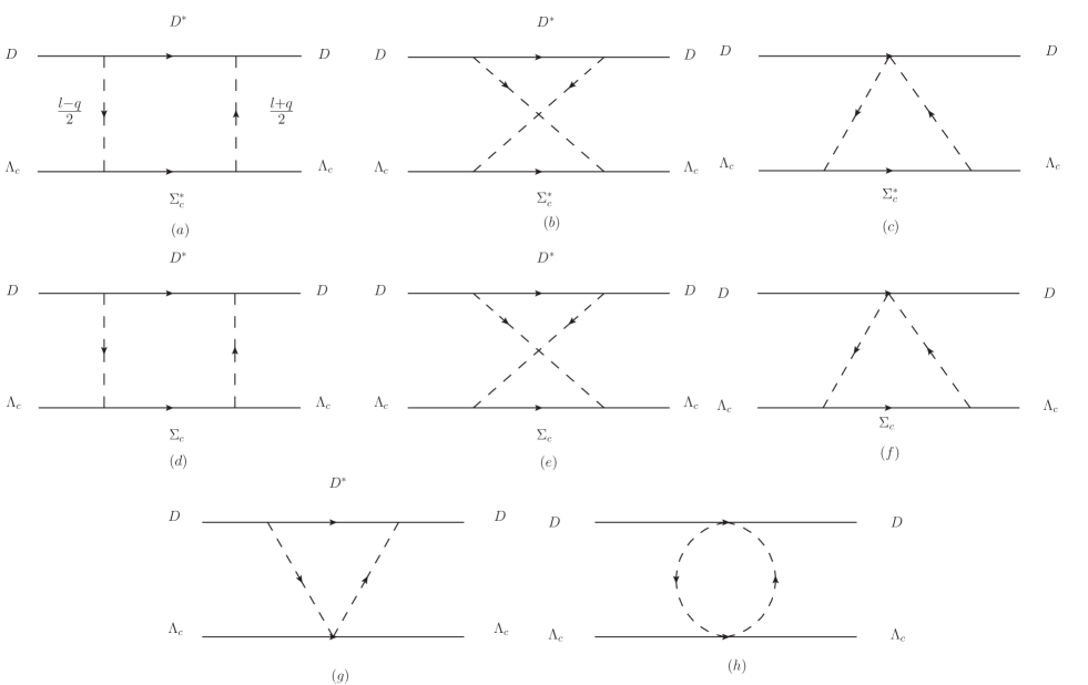
Figure 1: The Feynman Diagrams

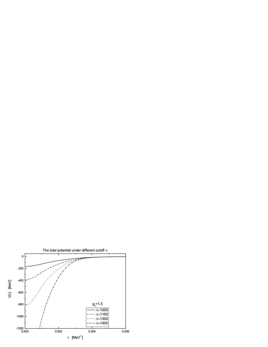
Figure 2: The total Potential of the $\Lambda_{c}-\bar{D}$ with various cutoff $\Lambda$(in units of MeV)

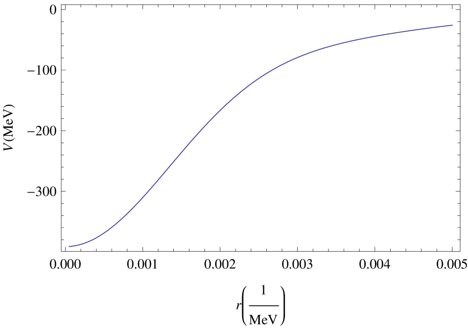
Figure 3: TPEP between nucleons with I=1,S=0 at $\Lambda=700MeV$

$\Lambda$[MeV]	$g_{4}$	$E_{bind}$[MeV]	$E=M-E_{bind}$[MeV]
1100	1.3	Not find	-
1150	1.3	-1.06	4150.20
1200	1.3	-8.25	4143.01
1250	1.3	-23.74	4127.42

Table.1 The bound state of the $\bar{D}-\Lambda_{c}$ in S-wave.

$\Lambda$ [MeV]	$g_{4}$	$E_{bind}$ [MeV]	$E=M-E_{bind}$ [MeV]
800	1.3	Not Found	-
850	1.3	-0.62	10899.08
900	1.3	-4.03	10895.67
950	1.3	-11.58	10888.12
1000	1.3	-25.05	10874.65

Table.2 The bound state of the $\bar{B}-\Lambda_{b}$ in S-wave.

3 Discussion and conclusion

In the cutoff scheme, the conclusion is inevitably sensitive to the cutoff. But the value of the cutoff cannot be known a priori. Because the long distance interaction is cut-off independent, we would like to know whether the short distance interaction is overestimated at the cut-off we choose. We can address this point by reference to the deuteron case. By using the TPEP between nucleons obtained in [24] plus OPEP, we repeat the process above and find a ${}^{3}S_{1}(I=0)$ deuteron bound state starts to appear at $\Lambda=700MeV$ consistent with [20].

An alternative approach s to study the nucleon’s interaction is given in ref. [28], where the authors use OPEP plus the potential from the leading order counter terms to fit the experimental data. The potential from the counter terms in the leading order of Chiral expansion is written as

$$V=C\delta^{3}(r).$$ (4)

In the channel ${}^{3}S_{1}(I=0)$, because the tensor part of OPEP is divergent at $r=0$ the situation is very complicated [28], so we make a comparison with the channel ${}^{1}S_{0}$where the value of the coefficient $C$ in (4) at $\Lambda=700MeV$ is $-(0.74\sim 1)\times 10^{-4}MeV^{-2}$ [28] [29]. Meanwhile, TPEP at $\Lambda=700MeV$ is shown in Fig.3. Analogously, if the potential in Fig.2 at $\Lambda=1000MeV$ is suitable for the heavy meson-baryon system, the coefficient $C$ of the corresponding potential (4) could be as large as $-1\times 10^{-4}MeV^{-2}$. Since we do not know $C$ for the heavy meson-baryon system, we refer to the KN system [26]. At $\Lambda=412MeV$, $C=-(2.6\sim 5.7)\times 10^{-4}MeV^{2}$.

The dependence of $C$ on $\Lambda$ may be complicated. In [29], the authors use a square well with radius R to smear the delta function of (4), then $C\sim 1/\Lambda$. This is approximately consistent with the result in [28]. Then, at $\Lambda=1GeV$, $C=-1\sim-2.3\times 10^{-4}MeV^{2}$ for the KN system. In QCD the interaction between two quarks is mass-independent, so the value of $C$ in the KN system may be referred to the $\bar{D}\Lambda_{c}$ system. Surely, $C$ is dependent on the masses of the meson and the baryon. In [26], the value of $C$ increases with increasing meson mass. If this tendency continues to the mass of the $D$ meson, $\Lambda$ is in the range $1000MeV\sim 1150MeV$.

From the above consideration, a bound state of the $B-\Lambda_{b}$ is optimistically expected, while for the $\bar{D}-\Lambda_{c}$ case the bound state is prudently expected and the situation may be dependent on the higher order corrections of the heavy quark expansion. Referring to the $X(3872)$ which is considered as a bound state of $D-\bar{D}^{*}$ as many authors suggested [27], if the $\bar{D}-\Lambda_{c}$ bound state ($\Lambda(4150)_{cc}$) exists, it could be produced in the channel $\Lambda_{b}\to\Lambda(4150)_{cc}K\to\eta_{c}NK$. The exact branching ratio of this channel is not easy to obtain, but the order of the branching ratio $\Lambda_{b}\to\Lambda(4150)_{cc}K$ may be roughly equal to that of $B\to X(3872)K$, because the scalar diquark in $\Lambda_{b}$ and the light quark in $B$ could be roughly considered as spin-decoupled spectators in heavy quark limit. This channel is expected to be seen in LHCb.

4 Acknowledgements

This work is supported partly by NNSFC under grant 11175153/A050202 and the Fundamental Research Funds for the Central Universities. We would like to thank Prof. Jifeng Yang for very helpful discussions.

5 Appendix

1. spin-$\frac{3}{2}$ digram in momentum space

$$V_{a}(\vec{q}) = \frac{-1}{4}(\frac{g}{f_{\pi}})^{2}(\frac{g_{4}}{f_{\pi}})^{2}\intop\frac{d^{3}l}{(2\pi)^{3}}(\vec{l}-\vec{q})\cdot(\vec{l}+\vec{q})(\vec{l}-\vec{q})\cdot(\vec{l}+\vec{q})\{\frac{1}{2(a+c)}[\frac{1}{\omega_{1}(\omega_{1}+a)}-\frac{1}{\omega_{2}(\omega_{2}+a)}]\frac{1}{\omega_{2}^{2}-\omega_{1}^{2}}$$

$$+\frac{1}{2(a+c)}[\frac{1}{\omega_{1}(\omega_{1}+c)}-\frac{1}{\omega_{2}(\omega_{2}+c)}]\frac{1}{\omega_{2}^{2}-\omega_{1}^{2}}\},$$

$$V_{b}(\vec{q}) = \frac{-1}{4}(\frac{g}{f_{\pi}})^{2}(\frac{g_{4}}{f_{\pi}})^{2}\intop\frac{d^{3}l}{(2\pi)^{3}}(\vec{l}-\vec{q})\cdot(\vec{l}+\vec{q})(\vec{l}-\vec{q})\cdot(\vec{l}+\vec{q})\{\frac{-1}{2(a-c)}[\frac{1}{\omega_{1}(\omega_{1}+a)}-\frac{1}{\omega_{2}(\omega_{2}+a)}]\frac{1}{\omega_{2}^{2}-\omega_{1}^{2}}$$

$$+\frac{1}{2(a-c)}[\frac{1}{\omega_{1}(\omega_{1}+c)}-\frac{1}{\omega_{2}(\omega_{2}+c)}]\frac{1}{\omega_{2}^{2}-\omega_{1}^{2}}\},$$

$$V_{c}(\vec{q}) = -\frac{1}{2}(\frac{g_{4}}{f_{\pi}})^{2}\frac{1}{f_{\pi}^{2}}\intop\frac{d^{3}l}{(2\pi)^{3}}(\vec{l}-\vec{q})\cdot(\vec{l}+\vec{q})(\frac{1}{\omega_{1}+c}-\frac{1}{\omega_{2}+c})\frac{1}{\omega_{2}^{2}-\omega_{1}^{2}},$$

where

$$\omega_{1}=\sqrt{(\vec{q}-\vec{l})^{2}+4m_{\pi}^{2}},$$

$$\omega_{2}=\sqrt{(\vec{q}+\vec{l})^{2}+4m_{\pi}^{2}},$$

and

$a=2(M_{D^{*}}-M_{D})$, $b=2(M_{\Sigma_{c}}-M_{\Lambda_{c}})$, $c=2(M_{\Sigma_{c}^{*}}-M_{\Lambda_{c}})$.

we transform above into coordinate space and obtain:

$$V_{a}(r) = \frac{-1}{4\pi}(\frac{g}{f_{\pi}})^{2}(\frac{g_{4}}{f_{\pi}})^{2}\frac{1}{a+c}\int d\lambda\frac{a}{a^{2}+\lambda^{2}}\left[\frac{2}{r^{2}}F^{{}^{\prime}}\left(\lambda,r\right)F^{{}^{\prime}}\left(\lambda,r\right)+F^{{}^{\prime\prime}}\left(\lambda,r\right)F^{{}^{\prime\prime}}\left(\lambda,r\right)\right]$$

$$+\frac{c}{c^{2}+\lambda^{2}}\left[\frac{2}{r^{2}}F^{{}^{\prime}}\left(\lambda,r\right)F^{{}^{\prime}}\left(\lambda,r\right)+F^{{}^{\prime\prime}}\left(\lambda,r\right)F^{{}^{\prime\prime}}\left(\lambda,r\right)\right],$$

$$V_{b}(r) = \frac{-1}{4\pi}(\frac{g}{f_{\pi}})^{2}(\frac{g_{4}}{f_{\pi}})^{2}\frac{1}{a-c}\int d\lambda\frac{-a}{a^{2}+\lambda^{2}}\left[\frac{2}{r^{2}}F^{{}^{\prime}}\left(\lambda,r\right)F^{{}^{\prime}}\left(\lambda,r\right)+F^{{}^{\prime\prime}}\left(\lambda,r\right)F^{{}^{\prime\prime}}\left(\lambda,r\right)\right]$$

$$+\frac{c}{c^{2}+\lambda^{2}}\left[\frac{2}{r^{2}}F^{{}^{\prime}}\left(\lambda,r\right)F^{{}^{\prime}}\left(\lambda,r\right)+F^{{}^{\prime\prime}}\left(\lambda,r\right)F^{{}^{\prime\prime}}\left(\lambda,r\right)\right],$$

$$V_{c}(r) = -\frac{1}{\pi}(\frac{g_{4}}{f_{\pi}})^{2}\frac{1}{f_{\pi}^{2}}\int d\lambda\frac{\lambda^{2}}{c^{2}+\lambda^{2}}\left(F^{{}^{\prime}}\left(\lambda,r\right)F^{{}^{\prime}}\left(\lambda,r\right)\right),$$

2.spin-$\frac{1}{2}$ in momentum space

$$V_{d}(\vec{q}) = \frac{-3}{8}(\frac{g}{f_{\pi}})^{2}(\frac{g_{2}}{f_{\pi}})^{2}\intop\frac{d^{3}l}{(2\pi)^{3}}(\vec{l}-\vec{q})\cdot(\vec{l}+\vec{q})(\vec{l}-\vec{q})\cdot(\vec{l}+\vec{q})\{\frac{1}{2(a+b)}[\frac{1}{\omega_{1}(\omega_{1}+a)}-\frac{1}{\omega_{2}(\omega_{2}+a)}]\frac{1}{\omega_{2}^{2}-\omega_{1}^{2}}$$

$$+\frac{1}{2(a+b)}[\frac{1}{\omega_{1}(\omega_{1}+b)}-\frac{1}{\omega_{2}(\omega_{2}+b)}]\frac{1}{\omega_{2}^{2}-\omega_{1}^{2}}\},$$

$$V_{e}(\vec{q}) = \frac{-3}{8}(\frac{g}{f_{\pi}})^{2}(\frac{g_{2}}{f_{\pi}})^{2}\intop\frac{d^{3}l}{(2\pi)^{3}}(\vec{l}-\vec{q})\cdot(\vec{l}+\vec{q})(\vec{l}-\vec{q})\cdot(\vec{l}+\vec{q})\{\frac{-1}{2(a-b)}[\frac{1}{\omega_{1}(\omega_{1}+a)}-\frac{1}{\omega_{2}(\omega_{2}+a)}]\frac{1}{\omega_{2}^{2}-\omega_{1}^{2}}$$

$$+\frac{1}{2(a-b)}[\frac{1}{\omega_{1}(\omega_{1}+b)}-\frac{1}{\omega_{2}(\omega_{2}+b)}]\frac{1}{\omega_{2}^{2}-\omega_{1}^{2}}\},$$

$$V_{f}(\vec{q}) = -\frac{3}{4}(\frac{g_{2}}{f_{\pi}})^{2}\frac{1}{f_{\pi}^{2}}\intop\frac{d^{3}l}{(2\pi)^{3}}(\vec{l}-\vec{q})\cdot(\vec{l}+\vec{q})(\frac{1}{\omega_{1}+b}-\frac{1}{\omega_{2}+b})\frac{1}{\omega_{2}^{2}-\omega_{1}^{2}},$$

and in coordinate space

$$V_{d}(r) = \frac{-3}{8\pi}(\frac{g}{f_{\pi}})^{2}(\frac{g_{2}}{f_{\pi}})^{2}\frac{1}{a+c}\int d\lambda\frac{a}{a^{2}+\lambda^{2}}\left[\frac{2}{r^{2}}F^{{}^{\prime}}\left(\lambda,r\right)F^{{}^{\prime}}\left(\lambda,r\right)+F^{{}^{\prime\prime}}\left(\lambda,r\right)F^{{}^{\prime\prime}}\left(\lambda,r\right)\right]$$

$$+\frac{b}{b^{2}+\lambda^{2}}\left[\frac{2}{r^{2}}F^{{}^{\prime}}\left(\lambda,r\right)F^{{}^{\prime}}\left(\lambda,r\right)+F^{{}^{\prime\prime}}\left(\lambda,r\right)F^{{}^{\prime\prime}}\left(\lambda,r\right)\right],$$

$$V_{e}(r) = \frac{-3}{8\pi}(\frac{g}{f_{\pi}})^{2}(\frac{g_{2}}{f_{\pi}})^{2}\frac{1}{a-c}\int d\lambda\frac{-a}{a^{2}+\lambda^{2}}\left[\frac{2}{r^{2}}F^{{}^{\prime}}\left(\lambda,r\right)F^{{}^{\prime}}\left(\lambda,r\right)+F^{{}^{\prime\prime}}\left(\lambda,r\right)F^{{}^{\prime\prime}}\left(\lambda,r\right)\right]$$

$$+\frac{b}{b^{2}+\lambda^{2}}\left[\frac{2}{r^{2}}F^{{}^{\prime}}\left(\lambda,r\right)F^{{}^{\prime}}\left(\lambda,r\right)+F^{{}^{\prime\prime}}\left(\lambda,r\right)F^{{}^{\prime\prime}}\left(\lambda,r\right)\right],$$

$$V_{f}(r) = -\frac{3}{2\pi}(\frac{g_{2}}{f_{\pi}})^{2}\frac{1}{f_{\pi}^{2}}\int d\lambda\frac{\lambda^{2}}{b^{2}+\lambda^{2}}\left(F^{{}^{\prime}}\left(\lambda,r\right)F^{{}^{\prime}}\left(\lambda,r\right)\right),$$

There is a triangle diagram(digram g in Fig.1) and a 4-veterx digram(digram h in Fig.1) without $\Sigma$ or $\Sigma^{*}$ propagator which provides :

$$V_{g}(\vec{q}) = -\frac{3}{4}(\frac{g}{f_{\pi}})^{2}\frac{1}{f_{\pi}^{2}}\intop\frac{d^{3}l}{(2\pi)^{3}}(\vec{l}-\vec{q})\cdot(\vec{l}+\vec{q})(\frac{1}{\omega_{1}+a}-\frac{1}{\omega_{2}+a})\frac{1}{\omega_{2}^{2}-\omega_{1}^{2}},$$

$$V_{h}(\vec{q}) = -\frac{3}{8}\frac{1}{f_{\pi}^{4}}\intop\frac{d^{3}l}{(2\pi)^{3}}\frac{1}{\omega_{1}+\omega_{2}},$$

$$V_{g}(r) = -\frac{3}{2\pi}(\frac{g}{f_{\pi}})^{2}\frac{1}{f_{\pi}^{2}}\int d\lambda\frac{\lambda^{2}}{a^{2}+\lambda^{2}}\left(F^{{}^{\prime}}\left(\lambda,r\right)F^{{}^{\prime}}\left(\lambda,r\right)\right),$$

$$V_{h}(r) = -\frac{3}{4\pi}\frac{1}{f_{\pi}^{4}}\int d\lambda\lambda^{2}F^{2}(\lambda,r).$$

The total potential of the $D-\Lambda_{c}$ is :

$$V(r) = V_{a}(r)+V_{b}(r)+V_{c}(r)+V_{d}(r)$$

$$+V_{e}(r)+V_{f}(r)+V_{g}(r)+V_{h}(r).$$

The Function $F(\lambda,r)$ used in the potential is defined as

$$F(\lambda,r) = e^{-\frac{\lambda^{2}}{\Lambda^{2}}}I_{2}(\sqrt{(2m_{\pi})^{2}+\lambda^{2}},r),$$

$$I_{2}(m,r) = \frac{m}{4\pi}\phi_{c}^{0}(m,r),$$

$$F^{\prime}(\lambda,r) = \displaystyle{\frac{d}{dr}F(\lambda,r)},$$

$$\phi_{c}^{0}(m,r) = e^{\frac{m^{2}}{\Lambda^{2}}}\left[e^{-mr}Erfc(-\frac{\Lambda r}{2}+\frac{m}{\Lambda})-e^{mr}Erfc(\frac{\Lambda r}{2}+\frac{m}{\Lambda})\right]\frac{1}{2mr}.$$

Here the function $Erfc(x)$ is the complementary error function. More details can be found in the Appendix of Ref [24].

References

• [1] J. D. Weinstein and N. Isgur, Phys. Rev. Lett.  48, 659 (1982). J. D. Weinstein and N. Isgur, Phys. Rev.  D 27, 588 (1983).
• [2] R.L. Jaffe, Phys.Rept. 409, 1 (2005).
• [3] Collaboration, T. Nakano et al., Phys. Rev. Lett.91 012002 (2003) .
• [4] D. E. Acosta et al. [CDF II Collaboration], Phys. Rev. Lett.  93, 072001 (2004); V. M. Abazov et al. [D0 Collaboration], Phys. Rev. Lett.  93, 162002 (2004); B. Aubert et al. [BABAR Collaboration], Phys. Rev.  D 71, 071103 (2005).
• [5] K. F. Chen et al. [Belle Collaboration], Phys. Rev. Lett. 100, 112001 (2008);I. Adachi et al. [Belle Collaboration], arXiv:1105.4583 [hep-ex];M. Karliner and H. J. Lipkin, arXiv:0802.0649 [hep-ph].
• [6] Marek Karliner1, Harry J. Lipkinb, and Nils A. Törnqvist, arXiv:1109.3472 [hep-ph].
• [7] S. Fleming, M. Kusunoki, T. Mehen and U. van Kolck , Phys.Rev. D76, 034006 (2007).
• [8] Aneesh V. Manohar, Mark B. Wise, Nucl.Phys.B399, 17 (1993)
• [9] S.O. Backman, G.E. Brown and J.A. Niskanen, Phys. Rep. 124, 1 (1985).
• [10] Frank E. Close and Philip R. Page. The D*0 anti-D0 threshold resonance. Phys.Lett., B578:119–123, 2004.
• [11] C. E. Thomas and F. E. Close, Phys. Rev.  D 78, 034007 (2008);
• [12] N. A. Tornqvist, Z. Phys.  C 61, 525 (1994) [arXiv:hep-ph/9310247].
• [13] Nils A. Tornqvist. Isospin breaking of the narrow charmonium state of Belle at 3872-MeV as a deuson. Phys.Lett., B590:209–215, 2004.
• [14] Kaiser, N., Siegel, P.B., Weise, W., Phys. Lett. B362, 23 (1995); Oset, E., Ramos, Nucl. Phys. A635, 99(1998); Oller, J.A., Oset, E., Ramos, A. Prog. Part. Nucl. Phys.45, 157 (2000); Oller, J.A., Meissner. Phys. Lett. B500, 263 (2001); Inoue, T., Oset, E., Vicente Vacas, M.J, Phys. Rev. C65, 035204 (2002); Garcia-Recio, C., Lutz, M.F.M., Nieves, J, Phys. Lett. B582, 49 (2004); Hyodo, T., Nam, S.I., Jido, D., Hosaka, A., Phys. Rev. C68, 018201 (2003).
• [15] M. Mattson et al., Phys. Rev.  Lett. 89, 112001 (2002).
• [16] M. B. Wise, Phys. Rev.  D 45, 2188 (1992).
• [17] T. M. Yan, H. Y. Cheng, C. Y. Cheung, G. L. Lin, Y. C. Lin and H. L. Yu, Phys. Rev.  D 46, 1148 (1992) [Erratum-ibid.  D 55, 5851 (1997)].
• [18] J. Phys.G 37, 075021(2010).
• [19] C. E. Thomas and F. E. Close, Phys. Rev.  D 78, 034007 (2008);
• [20] N. A. Tornqvist, Z. Phys.  C 61, 525 (1994) [arXiv:hep-ph/9310247].
• [21] I. W. Lee, A. Faessler, T. Gutsche and V. E. Lyubovitskij, Phys. Rev.  D 80, 094005 (2009) [arXiv:0910.1009 [hep-ph]].
• [22] C. Ordonez, L. Ray and U. van Kolck, Phys. Rev.  C 53, 2086 (1996) [arXiv:hep-ph/9511380].
• [23] N. Kaiser, R. Brockmann and W. Weise, Nucl. Phys.  A 625, 758 (1997)
• [24] T. A. Rijken, Annals Phys.  208, 253 (1991). T. A. Rijken and V. G. J. Stoks, Phys. Rev.  C 46, 73 (1992).
• [25] V. Bernard , Norbert Kaiser , Ulf-G. Meissner, Int.J.Mod.Phys.E4,193 (1995)
• [26] N. Kaiser, P.B. Siegel, W. Weise, Nucl.Phys. A594 325 (1995).
• [27] F. E. Close and P. R. Page, Phys. Lett.  B 578, 119 (2004); M. B. Voloshin, Phys. Lett.  B 579, 316 (2004);E. S. Swanson, Phys. Lett. B 588, 189 (2004); C. Y. Wong, Phys. Rev.  C 69, 055202 (2004);N. A. Tornqvist, Phys. Lett.  B 590, 209 (2004); C. E. Thomas and F. E. Close, Phys. Rev.  D 78, 034007 (2008); I. W. Lee, A. Faessler, T. Gutsche and V. E. Lyubovitskij, Phys. Rev.  D 80, 094005 (2009).
• [28] A. Nogga, R.G.E. Timmermans, U. van Kolck, Phys.Rev. C72,054006 (2005)
• [29] S.R. Beane, P.F. Bedaque, M.J. Savage, U. van Kolck, Nucl.Phys.A700 377 (2002).