The WHI Corona from Differential Emission Measure Tomography

Abstract

A three dimensional (3D) tomographic reconstruction of the local differential emission measure (LDEM) of the global solar corona during the whole heliosphere interval (WHI, Carrington rotation CR-2068) is presented, based on STEREO/EUVI images. We determine the 3D distribution of the electron density, mean temperature, and temperature spread, in the range of heliocentric heights 1.03 to 1.23 $R_{\odot}$. The reconstruction is complemented with a potential field source surface (PFSS) magnetic-field model. The streamer core, streamer legs, and subpolar regions are analyzed and compared to a similar analysis previously performed for CR-2077, very near the absolute minimum of the Solar Cycle 23. In each region, the typical values of density and temperature are similar in both periods. The WHI corona exhibits a streamer structure of relatively smaller volume and latitudinal extension than during CR-2077, with a global closed-to-open density contrast about 6% lower, and a somewhat more complex morphology. The average basal electron density is found to be about $2.23$ and $1.08\times 10^{8}\,{\rm cm^{-3}}$, in the streamer core and subpolar regions, respectively. The electron temperature is quite uniform over the analyzed height range, with average values of about 1.13 and 0.93 MK, in the streamer core and subpolar regions, respectively. Within the streamer closed region, both periods show higher temperatures at mid-latitudes and lower temperatures near the equator. Both periods show $\beta>1$ in the streamer core and $\beta<1$ in the surrounding open regions, with CR-2077 exhibiting a stronger contrast. Hydrostatic fits to the electron density are performed, and the scale height is compared to the LDEM mean electron temperature. Within the streamer core, the results are consistent with an isothermal hydrostatic plasma regime, with the temperatures of ions and electrons differing by up to about 10%. In the subpolar open regions, the results are consistent with departures from thermal equilibrium with $T_{\rm ions}>T_{\rm e}$ (and values of $T_{\rm ions}/T_{\rm e}$ up to about 1.5), and/or the presence of wave pressure mechanisms linear in the density.

1 Introduction

Advancing our understanding of the processes that heat and accelerate the coronal plasma now requires empirical knowledge of its three-dimensional (3D) structure. Coronal images are two-dimensional projections of the 3D structure, and a number of methods have been used to recover the 3D information from the 2D images. Available techniques include a variety of approaches, with diverse aims, strengths, and limitations. Towards this end, solar rotational tomography (SRT) constitutes a powerful empirical technique. Since the original work by Altschuler and Perry (1972), SRT has been developed and applied to polarized white-light image time series, allowing for the reconstruction of the 3D structure of the coronal electron number density. A modern implementation of SRT can be found in Frazin (2000) and Frazin and Janzen (2002), and a comprehensive review of its development in Frazin and Kamalabadi (2005).

One of the primary goals of NASA’s dual-spacecraft Solar Terrestrial Relations Observatory (STEREO) mission is precisely to determine the 3D structure of the corona (Kaiser et al., 2008). The Extreme UltraViolet Imager (EUVI) on the STEREO mission returns high-resolution ($1.6^{\prime\prime}$) narrow-band images centered over Fe emission lines at 171, 195, 284 Å, and the He ii 304 Å line (Howard et al., 2008). In this context, we have developed a novel technique, named differential emission measure tomography (DEMT). The technique was theoretically proposed by Frazin et al. (2005), and fully developed and applied to STEREO/EUVI data by Frazin et al. (2009; henceforth FVK09). DEMT takes advantage of the solar rotation to provide the multiple views required for tomography, as well as of the dual view angles provided by the STEREO spacecraft, the use of which allows for a reduced data-gathering time. Based on the input of EUV-image time series, DEMT produces maps of the 3D EUV emissivity, and a 3D DEM analysis free of 2D projection effects. As explained in FVK09, the first three moments of this local DEM (or LDEM) analysis give 3D maps of the electron density, the mean electron temperature, and the electron temperature spread. A major advantage of DEMT is that it obviates the need for ad-hoc modeling of specific structures of interest. Its main (current) limitation is the assumption of a static corona during the data-gathering process, implying that the reconstructions are reliable only in coronal regions populated by structures that are stable throughout their disk transit in the images. In contrast to other approaches, DEMT does not require background subtraction, and is global (i.e. it considers the entire corona), but it does not resolve individual loops.

In Vásquez et al. (2009), we published the first empirically derived 3D density and temperature structure of coronal-filament cavities, structures that are particularly interesting to study as filament eruptions are the progenitors of about 2/3 of all CMEs (Gibson et al., 2006). In Vásquez et al. (2010, VFM10 hereafter), we presented the first EUVI/STEREO DEMT analysis of the global corona, specifically for the period CR-2077, belonging to the Solar Cycle 23 extended solar-activity minimum period. In the present work, we develop a similar DEMT analysis for EUVI/STEREO data corresponding to the Whole Heliosphere Interval (WHI) period CR-2068 (20 March 2008, 01:14 UT through 16 April 08:05 UT). We also show a potential field source surface (PFSS) magnetic-field model based on the Michelson Doppler Imager (MDI/SOHO) magnetograms of the same period.

The Comparative Solar Minima (CSM) working group (WG), sponsored by Division II (Sun and Heliosphere) of the International Astronomical Union (IAU), focuses on the research of the coupled Sun–Earth system during solar minimum periods. It seeks to characterize the system at its most basic, “ground state” and aims to understand the degree and nature of variations within and between solar minima. In this context, we present here the results of the DEMT+PFSSM analysis of the WHI period. We discuss the implication of our model for the thermodynamical structure of the equatorial streamer belt, as well as for the surrounding magnetically open regions, both at the latitudes of the so-called “streamer legs”, and at the higher subpolar latitudes. To address the central interests of the IAU/CSM WG, we compare our results both with our similar analysis of CR-2077 (VFM10), as well as with results from studies of the Whole Sun Month period (WSM, CR-1913, 22 August through 18 September 1996), belonging to the previous solar-cycle minimum.

2 Summary of Differential Emission Measure Tomography

DEMTsec

We summarize in this section the main aspects of the DEMT methodology, a comprehensive description of the technique can be found in FVK09 and VFM10. DEMT consists of two phases. A first one applies solar rotational tomography (SRT) to a series of EUV images, the $K$ instrumental bands independently. As a result, the values of the $K$ filter band emissivities (FBEs) $\zeta_{k,i}$ are obtained at each tomographic grid cell (or voxel) $i$. The solution of the problem involves the application of regularization (or smoothing) methods to stabilize the inversion. The strength of the regularization is controlled by a single parameter [$p$], which is determined via the statistical procedure of cross validation.

In the second phase, a local DEM analysis is performed at each voxel using the local FBE values and assuming an optically thin plasma emission model, such as CHIANTI, for the computation of the different bands instrumental temperature responses. As a result, the LDEM distribution [$\xi_{i}(T)$] is obtained at each voxel [$i$]. The LDEM zeroth through second moments (Equations (4) through (6) in VFM10) give the voxels’ mean squared electron density [$N_{e,i}^{2}$], mean electron temperature [$T_{m,i}$], and squared electron temperature spread [$W_{T,i}^{2}$], respectively.

As the EUVI coronal bands are dominated by iron lines, their temperature responses are proportional to that element’s abundance. The root-mean-squared electron density [$N_{e,i}$] derived at each voxel is then inversely proportional to the squared root of the Fe abundance, assumed in this work to be uniform and equal to $\mathrm{[Fe]/[H]}=1.26\times 10^{-4}$ (Feldman et al., 1992), a low-FIP element abundance enhanced by a factor of about four respect to typical photospheric values (Grevesse and Sauval, 1998). The mean temperature [$T_{\mathrm{m}}$] and the temperature spread [$W_{T}$] are not affected by the assuumed Fe abundance.

As in our previous papers (FVK09; Vásquez et al. 2009; VFM10), for the FBE to LDEM inversion we assumed the Arnaud and Raymond (1992) ionization equilibrium calculations. In VFM10 we also performed an alternative inversion, based on the Mazzotta et al. (1998) ionization equilibrium model, to evaluate the typical uncertainty of LDEM moments due to the assumed model. The most affected quantity was the inferred temperature spread [$W_{T}$], with typical uncertainties of order 4% or less. The least-affected result was the mean electron temperature [$T_{\mathrm{m}}$], with uncertainties below 1%, while the inferred electron density [$\left<N_{e}^{2}\right>^{1/2}$] showed uncertainties of order 1% or less.

To quantify the uncertainty in the LDEM results due to the regularization level, in this work we performed two separate analyses, based on reconstructions using the mean and the minimum regularization levels obtained from the cross-validation study. We found the largest uncertainty in the temperature spread [$W_{T}$], with values in the range 3 to 9%. The uncertainty of the estimated electron density [$N_{\mathrm{e}}$] is in the range 2 to 5%. The least-affected result is the mean electron temperature [$T_{\mathrm{m}}$], with uncertainties below 2% everywhere.

We conclude this section with a brief discussion of the limits of validity of the technique’s results. As the SRT technique applied here does not account for the Sun’s temporal variations, rapid dynamics in the region of one voxel can cause artifacts in neighboring ones. Such artifacts include smearing and negative values of the reconstructed FBEs, or zero when the solution is constrained to positive values. These are called zero-density artifacts (ZDAs) and are similar in nature to those described by Frazin and Janzen (2002) in the context of white-light tomography. The voxels belonging to ZDA regions are excluded of the LDEM analysis. Active regions can present particularly rapid dynamics, and we do not analyze them here. For all voxels with no ZDAs, we use the inferred LDEM to forward-compute the three synthetic values of the FBE. The synthetic and reconstructed values agree within 1% in 77% of the voxels, and within 10% in 82% of the cases. For the analysis in Section resultsC, we only use the voxels where the achieved accuracy is within 1%.

Due to optical-depth issues in the EUV images close to the limb and the finite extent of the EUVI field of view, we view the tomographic reconstructions in this work as physically meaningful between heliocentric heights of 1.03 to 1.23 $R_{\odot}$. As with many optical instruments, the image measured by EUVI can be modeled as a convolution of the true solar image (as would be seen by an ideal telescope) with the instrument point spread function (PSF). The PSF has important consequences for the Sun’s fainter structures such as coronal holes (CHs) and emission at larger heights above the limb. Our preliminary analysis shows that, depending on the band, up to about 50% of the emission seen in CHs is due to the PSF. Since our deconvolution procedures are not yet ready for deployment, we do not analyze CHs here.

3 Observational Data, Tomography Parameters, and PFSS Model

OBS

We use EUVI/STEREO A and B data taken simultaneously during Carrington rotation (CR) 2068 (March 20 01:14 UT through 2008 April 16 08:05 UT 2008). In this period, the spacecraft were separated by an average of 47.7^∘, which allowed for the reconstruction to be performed with data gathered in about 24 days, a little less than the rotational period. The data set used consists of one-hour cadence images taken in the 2008 period between 20 March 00:00 UT and 12 April 23:59 UT. The total number of images used from each instrument and band is then about 576. During the observational period, the two spacecraft separation provided redundant observations over a range of about 265^∘. This resulted in a rich dataset, which provides much information for cross-validation purposes, as explained below.

The spherical computational grid covers the height range 1.00 to 1.25 $R_{\odot}$with 25 radial, 90 latitudinal, and 180 longitudinal bins, which gives a total number of about $4\times 10^{5}$ voxels, each with a uniform radial size of 0.01 $R_{\odot}$ and a uniform angular size of 2^∘ (in both latitude and longitude). It is not useful to constrain the tomographic problem with information taken from view angles separated by less than the grid angular resolution. Therefore, as the Sun rotates about 13.2^∘per 24-hour period, we time average the images in 6-hour wide bins, so that each time-averaged image is representative of views separated by about 3.3^∘. The total number of time-averaged images from each instrument and band is then about 96. Due to their high spatial resolution ($1.6^{\prime\prime}$ per pixel), to reduce both memory load and computational time, we spatially rebin the images by a factor of eight, bringing the original 2048 $\times$ 2048 pixel EUVI images down to 256 $\times$ 256. Thus the final images’ pixel size is about the same as the radial voxel dimension. Due to this spatial and temporal binning, the statistical noise in the EUVI images is greatly reduced.

Due to the relative spacecraft positions, the 24 days of collected data implied an angular range of 265^∘ in which both spacecraft saw the Sun from almost exactly the same viewpoint, although at different times. This resulted in a data set with 81 redundant image pairs. These redundant images give us the opportunity to determine the regularization parameter [$p$], by finding the value that best predicts one set of the redundant data, i.e. the 81 A or B images. This is only one way of choosing validation data, and Frazin and Janzen (2002) performed cross validation with single spacecraft data. Using the same cross-validation procedure described in VFM10, we obtained values in the range p = 0.35 $\pm$ 0.15, with the difference most like being due to the change in the spacecraft-separation angle The similar study for the reconstructions in Vásquez et al. (2009) and VFM10 gave comparable ranges, centered in the values $p=0.9$ and $p=1.77$, respectively. The results presented in this work correspond to $p=0.5$, using all images from both spacecraft. In Section results we quantify the uncertainty of the LDEM moments due to that of the regularization parameter. Regularization parameter selection and other uncertainty quantification will be given a comprehensive treatment in a forthcoming publication.

We made use of a potential field source surface (PFSS) model of the coronal magnetic field (Altschuler et al., 1977). The source-surface height was set at $R_{\rm SS}$ = 2.5 $R_{\odot}$, and the lower boundary condition prescribed by the synoptic magnetogram for CR-2068 provided by MDI/SOHO. We traced the magnetic-field lines through the tomographic computational grid, producing the run of LDEM distributions along each field line. This also allowed classification of the voxels as belonging to magnetically open or closed regions of the PFSS model.

4 Results

results

4.1 Analysis of the 3D Reconstructions

resultsA

As an example of the 3D tomographic reconstruction of the emissivity, Figure FBE_maps_1 shows the Carrington maps of $\zeta_{k}$ at height 1.035 $R_{\odot}$, for the three coronal Fe bands of 171, 195, and 284 Å. The black voxels are the ZDAs described in Section 2, which occupy 9% of the reconstructed volume. The overplotted solid-thin curves are contour levels of the PFSSM magnetic strength [$B$], in steps of 1.0 G. The white (black) contours represent outward (inward) oriented magnetic field. The overplotted solid-thick black curves indicate the boundary between the magnetically open and closed regions. The reconstructed FBEs exhibit larger values within the PFSS model’s magnetically closed regions, and lower values in the open regions. The peak emission is located within the active region (AR) complex in the southern hemisphere and near the Equator, in the longitudinal range [190^∘, 270^∘]. The PFSS model considers latitudes up to $\pm 81.5^{\circ}$, beyond which the magnetogram was extrapolated. At the larger latitudes, the MDI data shows an asymmetry between both hemispheres, with the northern part exhibiting a decreasing magnetic strength beyond latitude +75^∘. This gives rise to artificial magnetically neutral locations in the extrapolated highest latitudes of the northern hemisphere, producing an artifact of $\beta>1$ values at all longitudes near the North Pole (see Figure beta_maps and its discussion below.

In the following discussion, we identify the magnetically closed region as the equatorial streamer core. The magnetically open field lines immediately surrounding the equatorial streamer core are known as the streamer legs, where the O VI 1032 Å intensity relative to H I 1216 Å is often seen to be higher than in the core, above 1.5 $R_{\odot}$, as seen for example in Raymond et al. (1997) and Strachan et al. (2002). A geometrical sketch of the streamer core and leg structure can be found in Figure 1 of Nerney & Suess (2005). The magnetically open latitudes just outside of the streamer legs, up to about latitudes $\pm 75^{\circ}$, will be referred to as the subpolar regions. Beyond that latitude we curretly avoid analysis of results due to the importance of PSF contamination in CHs (deconvolution has not yet been implemented). Figure context displays the solar corona on 2008 March 24 at approximately 19:00 UT. In those images the west and east limb longitudes are about 30^∘ and 210^∘, respectively. In the EIT image, the east limb just hides the foot location of the easternmost AR seen between longitudes 200^∘and 210^∘ in the Carrington maps of Figure FBE_maps_1. In the west limb, the Mauna Loa Solar Observatory (MLSO) MkIV white light image shows the streamer belt between heliocentric heights 1.25 and 2.35 $R_{\odot}$, around longitude 30^∘. That location is surrounded by a very wide longitude range of quiet sun corona, at least 90^∘ wide in both the eastward and westward directions (see Figure 1). The Large Angle and Spectrometric Coronagraph (LASCO/SOHO) C2 image to the right shows the extended streamer structure above 2.3 $R_{\odot}$. Being a period of minimum activity, open regions are usually confined to the higher latitudes, and characterized by a lower emissivity. The PFSS model open/closed boundary shows an isolated low-latitude open region, centered at longitude 265^∘ and latitude +5^∘ at 1.035 $R_{\odot}$. In the southern hemisphere, the open regions extend to low latitudes within the longitude range [100^∘, 200^∘], reaching a maximum latitude of $-10^{\circ}$ around longitude 200^∘.

Figure LDEM_Ne_maps shows the Carrington maps of the 3D distribution of the electron density [$\left<N_{e}^{2}\right>_{i}^{1/2}$, in $10^{8}\,{\rm cm}^{-3}$ units], at heights 1.035, 1.075, and 1.135 $R_{\odot}$. For the same heights, Figures LDEM_Tm_maps and LDEM_WT_maps show the Carrington maps of the mean temperature [$T_{m,i}$, MK] and the temperature spread [$W_{T,i}$, MK], respectively. In all these Figures, we overplot PFSSM magnetic strength [$B$] contour levels (solid-thin black and white curves), as well as the magnetically open/closed region boundaries (solid-thick black curves). The black voxels in the different maps correspond to undetermined LDEM locations due to the presence of a ZDA for at least one of the bands, which represent 9% of the total number of voxels.

Figure LDEM_Ne_maps shows that the largest densities are found in the ARs. In order to highlight the quiescent structure, we threshold the maximum density displayed at each height, as indicated by the respective color scales. The peak densities in the AR complex are 9.0, 6.3, and 3.9 $\times 10^{8}\,{\rm cm}^{-3}$ at 1.035, 1.075, and 1.135 $R_{\odot}$, respectively.

At all heights, the PFSSM closed region is populated by densities clearly enhanced with respect to the open regions, consistent with its identification as the streamer core. A notable characteristic of these maps is that, at all heights, the PFSSM open/closed boundary very accurately demarcates the location of the transition between streamer to subpolar density levels (red to green). This good morphological match between the structures derived from the tomographic and the PFSSM analyses, is similar to what we found for CR-2077 (VFM10), compared to which the topology found here is more complex due to a relatively higher level of activity. At all heights, the magnetically open subpolar regions are characterized by densities of order half of those typically found within the quiescent streamer core, which are typically in the range $1.5-0.5\times 10^{8}\,{\rm cm}^{-3}$ in the height range we study.

Figure LDEM_Tm_maps shows that the largest temperatures are found in the ARs. In order to highlight the quiescent structure, we threshold the maximum temperature displayed at each height, as indicated by the respective color scales. The peak $T_{\mathrm{m}}$ values in the AR complex are 2.5, 2.4, and 2.9 MK at 1.035, 1,075, and 1.135 $R_{\odot}$, respectively. The Carrington maps show that the most quiet longitudes of the streamer core, away from the AR complex, are characterized by lower temperatures [$T_{\mathrm{m}}$] near the Equator than at higher latitudes. These higher temperature regions can typically reach $T_{\mathrm{m}}=1.4$ MK, being 40% larger than average streamer core equatorial values. The overplotted magnetic-field strength contour levels reveal that all high $T_{\mathrm{m}}$ (yellow) areas are located along and around polarity inversion lines, as well as close to the open/closed boundary. Note also that, in most cases, these higher-temperature regions do not extend into the magnetically open parts, and the open/closed boundary generally matches their high latitude limit. The characteristics of the coronal temperature structure described in this paragraph are common to the DEMT results of the CR-2077 period (VFM10).

Figure LDEM_WT_maps shows that the largest values of the LDEM electron temperature spread [$W_{T}$] are found in the ARs, where the peak value is around 0.85 MK at all heights. In order to highlight the quiescent structure, we threshold the maximum displayed value at each height, as indicated by the respective color scales. Figure LDEM_WT_maps shows that the distribution of $W_{T}$ is quite complex, not clearly correlated with the other two moments, except for the AR complex, outside of which the temperature spread values are typically in the range 0.1 to 0.4 MK. Unlike for the other two moments, the magnetically open/closed boundary is not characterized by a clear change of temperature spread. The lowest values are seen in the open regions, but generally away of the open/closed boundary, at somewhat higher latitudes. This has been found more clearly in our analysis of the period CR-2077 (VFM10). In that period, characterized by a much simpler coronal structure, we found that the change from higher to lower $W_{T}$ values systematically occurred some degrees in latitude outside the magnetically open/closed boundary.

Figure 3Dview shows a 3D view of the CR-2068 PFSS model. Some representative open and closed magnetic-field lines are drawn in white. The red and orange regions are LDEM $T_{\mathrm{m}}$ isosurfaces of 2 and 1 MK, respectively. The inner spherical surface shows the LDEM $N_{\mathrm{e}}$ at 1.04 $R_{\odot}$, with the displayed color scale. The 2 MK region corresponds to the AR complex. Figure LDEM_Tm_maps shows that at all heights in the northern hemisphere, the magnetically open/closed boundary and its surrounding latitudes show $T_{\mathrm{m}}>1\,{\rm MK}$. On the magnetically open side of the boundary, the 1 MK level (orange voxels) is achieved at latitudes right outside the open/closed boundary. On the magnetically closed side of the boundary, the 1 MK level is achieved at latitudes considerably lower than those of the open/closed boundary. Consistently, the orange isosurface of the 3D view leaves then a wide “empty” region just inside of the magnetically open/closed boundary, and the border of the orange isosurface in the northern polar region indicates the open/closed boundary quite accurately.

With the tomographic LDEM moments $\left<N_{e}^{2}\right>^{1/2}$ and $T_{\mathrm{m}}$, as measures of the electron density and temperature, respectively, and the PFSSM magnetic strength [$B$], we estimate the plasma $\beta=16\pi\left<N_{e}^{2}\right>^{1/2}k_{B}T_{\mathrm{m}}/B^{2}$, where we have approximated the total thermal pressure as $p\approx 2N_{\mathrm{e}}k_{B}T_{\rm e}$. Figure beta_maps shows Carrington maps of $\beta$ at heights 1.035, 1.075, and 1.135 $R_{\odot}$, thresholded at a maximum value of five. It is interesting to note how $\beta>1$ values are typical of the streamer core region, except for the ARs complex where the magnetic strength is very high. The largest $\beta$ values within the streamer core are of order 5 to 10, corresponding to the lowest magnetic-strength values near polarity inversion zones. Throughout the magnetically open regions $\beta<1$, except for the artifacts in the northern CH region mentioned above.

4.2 Analysis of Results for Quiet Sun Open and Closed Magnetic Structures

resultsC

We analyze here the physical properties of quiet-Sun regions as derived with the LDEM analysis, both in the streamer core and in the surrounding magnetically open regions. In each panel of Figure FBE_maps_1, the four black boxes highlight the quiet-Sun regions selected for the analysis. In the equatorial region we selected the streamer core between longitudes 0^∘ and 160^∘, and latitudes -20^∘ to +20^∘, a region that we name here SC. The other selected regions surround the open/closed boundary, and we name them here: $R_{1}$ (southern hemisphere, between longitudes 0^∘ and 100^∘, and latitudes -70^∘ to -40^∘), $R_{2}$ (northern hemisphere, between longitudes 0^∘ and 100^∘, and latitudes 40^∘ to 70^∘), and $R_{3}$ (northern hemisphere, between longitudes 120^∘ and 220^∘, and latitudes 45^∘ to 75^∘). Note that in each of these regions the open/closed boundary occupies the intermediate latitude range. The horizontal black lines within each of these three regions delimit subregions that are discussed below.

In order to characterize the plasma properties in the streamer/subpolar transition, we analyze the LDEM results as a function of height when averaged over the regions $R_{i}$ (i=1,2,3) and the streamer core. Within each of the regions $R_{i}$, we have divided our analysis in three different latitude sub-ranges, that we name here as $R_{i}$-C, $R_{i}$-B and $R_{i}$-O. Sub-regions $R_{i}$-C consist of the lowest 4^∘ in latitude of each region, sampling data representative of their magnetically closed sector, inside the streamer core. Sub-regions $R_{i}$-O consist of the largest 4^∘ in latitude of each region, sampling data representative of their magnetically open part, outside the streamer core. Sub-regions $R_{i}$-B consist of the middle 10^∘ in latitude of each region, sampling data representative of the open/closed boundary zone, mixing data from regions immediately inside and outside the open/closed boundary. For each of these regions, Figures tomo_height_Ne to tomo_height_WT show the average dependence with height of the LDEM electron density [$N_{e}(r)$, which we will denote $\left<N_{e}^{2}\right>^{1/2}$ hereafter], the mean electron temperature [$T_{\mathrm{m}}(r)$], and the electron temperature spread [$W_{T}(r)$]. In regions $R_{i}$ we use diamonds to display data from subregions $R_{i}$-C, triangles for $R_{i}$-B, and squares for $R_{i}$-O.

The solid curves in the density plots show the unweighted least-squares fit to the tomographic data in the height range 1.035 to 1.195 $R_{\odot}$, of the form

$$\ilabel{static}N_{e}(r)=N_{e0}\ {\rm exp}\left[-\,(h/\lambda_{{\rm N}})\,/\,(r/R_{\odot})\right]$$ (1)

where $r$ is the heliocentric height, $h=r-R_{\odot}$, $\lambda_{{\rm N}}$ is the density scale height, and $N_{e0}$ is the electron density at $r=1R_{\odot}$. Equation (static) represents the hydrostatic solution for a plasma with a uniform temperature. In both the streamer legs and the subpolar open regions, at the very low height range that we analyze, the the inertial effects of the bulk outflow velocity can be safely neglected. In a fully ionized corona, with a helium abundance $a\equiv N({\rm He})/N({\rm H})$, the mean atomic weight per electron is $\mu=(1+4a)/(1+2a)$, in terms of which the plasma mass density is $\rho=\mu m_{H}N_{e}$. We set $a=0.08$, as in the CHIANTI coronal abundances set (Feldman et al., 1992) we used to compute the DEM kernels. The fitted scale $\lambda_{{\rm N}}$ determines $T_{\rm fit}$ and is given by $\lambda_{{\rm N}}=k_{B}T_{\rm fit}/\left(\mu m_{H}g_{\rm s}\right)$, where $g_{\rm s}\equiv GM_{\rm s}/R_{\odot}^{2}$, and

$$\ilabel{Tfit}T_{\rm fit}\equiv T_{\rm e}+T_{\rm H}/(1+2a)+a\ T_{\rm He}/(1+2a).$$ (2)

In case of isothermality among the different species, one obtains $T_{\rm fit}=T_{\rm e}/b$, with $b\equiv(1+2a)/(2+3a)\approx 0.52$.

In Table tab1, we show the statistics of the hydrostatic fit and LDEM for the selected Regions (rows). In the different columns we tabulate the fit’s basal density $N_{e0}$, scale height $\lambda_{{\rm N}}$, and electron temperature $bT_{\rm fit}$ derived from Equation (Tfit) assuming species are isothermal. We also give the average $\left<T_{\mathrm{m}}\right>$ and variance $\sigma^{2}_{T_{\mathrm{m}}}$ of $T_{\mathrm{m}}(r)$ in the analyzed height range, the temperature difference $\Delta T\equiv bT_{\rm fit}-\left<T_{\mathrm{m}}\right>$, and the average $\left<W_{T}\right>$ and and variance $\sigma^{2}_{W_{T}}$ of $W_{T}(r)$ in the analyzed height range.

Region	$N_{e0}$	$\lambda_{{\rm N}}$	$bT_{\rm fit}$	$\left<T_{\mathrm{m}}\right>$	$\frac{\sqrt{\sigma^{2}_{T_{\mathrm{m}}}}}{\left<T_{\mathrm{m}}\right>}$	$\frac{\Delta T}{\left<T_{\mathrm{m}}\right>}$	$\left<W_{T}\right>$	$\frac{\sqrt{\sigma^{2}_{W_{T}}}}{\left<W_{T}\right>}$
	[$10^{8}{\rm cm^{-3}}$]	[$R_{\odot}$]	[MK]	[MK]
SC	2.23	0.0855	1.16	1.10	0.04	$+$0.06	0.28	0.04
$R_{1}$-C	1.99	0.0824	1.12	1.06	0.02	$+$0.06	0.26	0.10
$R_{1}$-B	1.49	0.0805	1.10	0.95	0.04	$+$0.15	0.23	0.16
$R_{1}$-O	1.04	0.0844	1.15	0.93	0.06	$+$0.23	0.21	0.23
$R_{2}$-C	2.00	0.0873	1.19	1.19	0.04	$-$0.01	0.29	0.03
$R_{2}$-B	1.90	0.0784	1.07	1.19	0.02	$-$0.10	0.29	0.04
$R_{2}$-O	1.20	0.0786	1.07	0.95	0.05	$+$0.12	0.24	0.31
$R_{3}$-C	1.98	0.0875	1.19	1.27	0.05	$-$0.06	0.27	0.03
$R_{3}$-B	1.72	0.0784	1.07	1.22	0.03	$-$0.12	0.29	0.06
$R_{3}$-O	1.00	0.0859	1.17	0.95	0.06	$+$0.23	0.23	0.19

Table 1.: Statistics of the hydrostatic fit and LDEM analysis as a function of height for the selected regions, using regularization parameter $p=0.5$.tab1

The hydrostatic fits are a quite accurate description of the observed dependence with height in each region, with squared correlation coefficient values in the range 0.963 to 0.997. We note also that, in all cases, the variability of the LDEM electron mean temperature, measured by $\sqrt{\sigma^{2}_{T_{\mathrm{m}}}}/\left<T_{\mathrm{m}}\right>$, is 6% or lower, so each region exhibits a quite uniform temperature, as assumed by the hydrostatic fits (though there can be temperature variations on large spatial scales as seen in Figure LDEM_Tm_maps).

In the closed regions, the match between $bT_{\rm fit}$ and $\left<T_{\mathrm{m}}\right>$ is best, being within 6% or better in the streamer core and the three $R_{i}$-C regions. This is consistent with a plasma regime close to isothermal hydrostatic equilibrium throughout the whole streamer core region. Note that in the three $R_{i}$-O regions, the difference $\Delta T$ is clearly larger than in the $R_{i}$-C regions, reaching values of order 23%. This is an indication that, in open regions immediately surrounding the streamer, the plasma departs from the isothermal hydrostatic regime. Consistently with this picture, within each region the $R_{i}$-B sub-region, which mixes plasma from both open and closed regions, shows intermediate degrees of agreement between both temperatures.

Where the value of $\Delta T$ is larger, one possibility is that other pressure mechanisms are acting, modifying the scale height respect to that due to the thermal pressure only. If so, the excellent goodness-of-fit everywhere, as measured by $R^{2}$, suggests that such other processes must be linear in the plasma density. Another possibility is that the isothermality among the different species is not met. Equation (Tfit) implies that if the ions are hotter than the electrons then $bT_{\rm fit}>T_{\rm e}$. Hence, taking the LDEM $T_{\mathrm{m}}$ as a measure of the true electron temperature, the fact that in all $R_{i}$-O regions we find $\Delta T=bT_{\rm fit}-\left<T_{\mathrm{m}}\right>>0$ implies that the ions are hotter than the electrons in the open regions. Replacing $T_{\rm e}=\left<T_{\mathrm{m}}\right>$ in Equation (Tfit), we solve for $T_{\rm H}$, and obtain

$$\frac{T_{\rm H}}{\left<T_{\mathrm{m}}\right>}=\left(\frac{\Delta T}{\left<T_{\mathrm{m}}\right>}+\frac{1+a}{2+3a}\right)\,\left(\frac{2+3a}{1+a\,T_{\rm He}/T_{\rm H}}\right)\,\approx 1+2\,\frac{\Delta T}{\left<T_{\mathrm{m}}\right>}\,,$$ (3)

where the last approximation is valid for negligible coronal He abundance, and clearly shows that if $\Delta T/\left<T_{\mathrm{m}}\right>>0$ then $T_{\rm H}>\left<T_{\mathrm{m}}\right>$. Assuming $T_{\rm He}=T_{\rm H}\equiv T_{\rm ions}$, the maximum values $\Delta T/\left<T_{\mathrm{m}}\right>=+0.23$ we found in regions $R_{1}$-O and $R_{3}$-O, imply $T_{\rm ions}/\left<T_{\mathrm{m}}\right>\approx 1.48$. In the quiet-Sun regions SC and $R_{i}$-C, within the magnetically closed streamer core, we found values $\Delta T/\left<T_{\mathrm{m}}\right>=\pm 0.06$, which implies a temperature ratio in the range $T_{\rm ions}/\left<T_{\mathrm{m}}\right>\approx 1.0\pm 0.12$.

The analysis summarized in Table tab1 shows the average dependence with height of the electron density for each selected region, not considering the individual magnetic-field lines. In order to perform an analysis more consistent with the magnetic geometry of the PFSS model, we traced individual field lines through the tomographic computational grid. For each field line $i$, we determined the dependences of the LDEM $N_{\mathrm{e}}^{(i)}(r)$ and $T_{\mathrm{m}}^{(i)}(r)$, in the height range 1.03 to 1.2 $R_{\odot}$. For every density profile $N_{\mathrm{e}}^{(i)}(r)$, we performed a least-squares hydrostatic fit of the form given by Equation (static). The hydrostatic-fit temperature of each line [$T_{\rm fit}^{(i)}$] was then compared with the respective LDEM electron temperature averaged along the line, $\left<T_{\mathrm{m}}\right>^{(i)}$.

Figure linetrace_R1 shows a statistical analysis of the results for the closed (left) and open (right) field lines in region $R_{1}$. The top panels show the histograms of $\left<T_{\mathrm{m}}\right>^{(i)}$ along each field line. The middle panels show the histograms of the difference $\Delta T^{(i)}\equiv bT_{\rm fit}^{(i)}-\left<T_{\mathrm{m}}\right>^{(i)}$ for each field line. The bottom panels shows the scatter plots of $bT_{\rm fit}^{(i)}$ versus $\left<T_{\mathrm{m}}\right>^{(i)}$. The top panels show that the two populations have clearly different mean values, with the closed region one being $11\%$ larger. The middle panels show a mean fractional difference $\Delta T^{(i)}/\left<T_{\mathrm{m}}\right>^{(i)}$ of about $+6\%$ for the closed field lines, and $+21\%$ for the open field lines. These numbers match very accurately those of $\Delta T/\left<T_{\mathrm{m}}\right>$ in Table tab1 for $R_{1}$-C and $R_{1}$-O, which are $+6\%$ and $+23\%$, respectively.

We performed the same analyses for regions $R_{2}$ and $R_{3}$, and the results are shown in Figures linetrace_R2 and linetrace_R3, respectively. For the closed field lines, the top-left histograms show a mean fractional difference [$\Delta T^{(i)}/\left<T_{\mathrm{m}}\right>^{(i)}$] of $-4$ and $-9\%$, for regions $R_{2}$ and $R_{3}$ respectively. These numbers are quite similar to (and consistent in sign with) those of $\Delta T/\left<T_{\mathrm{m}}\right>$ in Table tab1 for $R_{2}$-C and $R_{3}$-C, which are $-1$ and $-6\%$ respectively. A negative value for $\Delta T^{(i)}$ may be a direct indicator that $T_{\rm e}>T_{\rm ions}$, but it could also mean that the loops are inherently dynamic on time scales not resolved by the method.

The top-right histogram of Figure linetrace_R2 shows two distinct populations of open field lines, centered around different mean temperatures, larger and lower than $\approx$1 MK. A similar characteristic is seen in the top-right histogram of Figure linetrace_R3. Consistently, in the top panel of Figure LDEM_Tm_maps the open part of region $R_{2}$ shows $T_{\mathrm{m}}>1$ MK (yellow) and $<1$ MK (orange) voxels, and the same is seen in the open part of region $R_{3}$. As regions $R_{2}$-O and $R_{3}$-O are almost exclusively populated by $T_{\mathrm{m}}<1$ MK voxels, to compare with their results in Table 1 we consider now only the population $\left<T_{\mathrm{m}}\right>^{(i)}<1$ MK of the corresponding histogram. For that subset we find a mean fractional difference $\Delta T^{(i)}/\left<T_{\mathrm{m}}\right>^{(i)}$ of order $+14\%$, both in region $R_{2}$ and $R_{3}$. This value compares quite well with the value $\Delta T/\left<T_{\mathrm{m}}\right>=+12\%$ in Table tab1 for $R_{2}$-O, and is somewhat smaller than the value $\Delta T/\left<T_{\mathrm{m}}\right>=+23\%$ value for $R_{3}$-O. In summary, both the results of Table 1 and of the histograms for the magnetic structures, reveal a consistent trend for the open subpolar regions to show larger $\Delta T/\left<T_{\mathrm{m}}\right>$ values than the closed regions within the streamer core.

4.3 Comparative Quantitative Analysis of CR-2068 and CR-2077

resultsB

As qualitatively described in the previous section, the DEMT analysis of CR-2068 and CR-2077 (VFM10) reveals many similarities between both periods, as well as differences. We include in this section a quantitative comparison of the two periods, both belonging to the Solar Cycle 23 extended minimum phase. The WHI CR-2068 (March – April 2008) period showed increased magnetic activity with respect to CR-2077 (November – December 2008). This is due to the later being closer to the absolute minimum of sunspot number for Solar Cycle 23, which occurred in December 2008 according to the National Oceanic and Atmospheric Administration Space Weather Prediction Center (http://www.swpc.noaa.gov/SolarCycle). This is clearly manifested by the presence of the AR complex in the southern hemisphere near the equator in CR-2068, that shows an overall more complex magnetic topology than CR-2077.

We begin by quantifying the relative difference in the two Carrington rotations in a global way. Since the reconstructions from both periods are subject to extremely similar systematic errors, the relative differences between the two periods can be quantified much more precisely than absolute quantities. Inspection of the FBE Carrington maps for CR-2068 and CR-2077 (VFM10) shows that both periods exhibit the most quiet characteristics throughout the CL range 0 to 160^∘. We use that range for this global analysis, as at higher CLs CR-2068 shows an AR complex. We also limit the analysis to the latitudinal range -75 to +75^∘, to avoid the PSF contaminated regions of the CHs. In this coordinate range, and with the aid of the PFSS model, we label the tomographic grid voxels as open or closed, belonging to the streamer core and streamer-leg/subpolar regions, respectively.

For each given physical quantity of interest $Q$, we computed its average value at a given height in the open and closed regions for both periods. We then computed the ratio $R_{Q}\equiv\left<Q\right>_{\rm CR-2068}/\left<Q\right>_{\rm CR-2077}$, for the open and closed regions separately. At three different heights of the tomographic grid (spherical shells of width $\Delta r=0.01R_{\odot}$), Table tab2 shows, for each region, the ratios of: the areas [$A$], the average FBEs [$\zeta_{k}$] in each of the three coronal bands, the average LDEM electron density [$N_{e}$], the total mass in the shell [$M=\mu m_{H}N_{e}A\Delta r$], the average electron mean temperature [$T_{\mathrm{m}}$], and the average electron temperature spread [$W_{T}$].

Height [$R_{\odot}$]	$R_{A}$	$R_{\zeta 171}$	$R_{\zeta 195}$	$R_{\zeta 284}$	$R_{N_{e}}$	$R_{M}$	$R_{Tm}$	$R_{W_{T}}$
Closed Region
1.035	0.96	1.01	0.93	0.94	0.99	0.96	0.98	1.04
1.075	0.93	1.05	0.93	0.90	1.00	0.92	0.97	1.00
1.135	0.90	1.05	0.98	0.89	1.01	0.90	0.99	1.07
Open Region
1.035	1.24	1.09	0.98	0.75	1.07	1.32	1.07	1.16
1.075	1.36	1.10	0.98	0.74	1.06	1.45	1.03	1.05
1.135	1.38	1.08	0.94	0.75	1.04	1.44	1.01	1.09

Table 2.: Ratios $R_{Q}\equiv\left<Q\right>_{\rm CR-2068}/\left<Q\right>_{\rm CR-2077}$ of different quantities (see text), for the open and closed regions separately, at three heights. tab2

In the three analyzed heights, the CR-2068 closed (streamer) area is 4 to 11% smaller than during CR-2077. This is consistent with the slightly larger latitudinal extent of the CR-2077 streamer core, which can also be seen by comparing the location of the open/closed boundaries in Figure 1 with the corresponding Figure 1 in VFM10. The average electron density in both periods is about the same, and the lower total mass of the CR-2068 streamer is then due to its smaller area. The average electron temperature in the CR-2068 streamer is 2% lower, while the temperature spread is about 4% larger.

In the three analyzed heights, the area of the CR-2068 open regions (which we recall it includes only up to latitudes $\pm 75^{\circ}$) is 24 to 38% larger than during CR-2077, while the average electron density is about $\approx$6% larger. The larger total mass of the CR-2068 open regions is then due to a contribution of both factors, being the larger areas the dominant one. The average electron temperature in the CR-2068 open regions is about 4% larger, while the temperature spread is about 10% larger.

Combining DEMT with the PFSS model, we computed at each voxel the plasma $\beta$ parameter for both periods. As shown in Figure beta_maps, some localized regions show very high (say $\beta>5$) values within the closed region. As the great majority (more than 80%) of the voxels have $\beta<5$, by taking the median (instead of the mean) of the $\beta$ value in each region we obtain a representative value not considering the highest values. For the considered range of coordinates, Table tab3 shows the typical value of $\beta$ for the closed (C) and open (O) regions. As already pointed out, the plasma $\beta$ is of order one within the streamer core, and much less than one in the surrounding open regions, with both periods showing a similar scenario. The most notable difference between both periods is found in the open regions, for which CR-2077 shows lower values relative to CR-2068. We find then a slightly enhanced closed-to-open $\beta$ contrast for CR-2077 respect to CR-2068.

$r/R_{\odot}$	C-2068	C-2077	O-2068	O-2077
1.035	0.99	1.19	0.14	0.08
1.075	1.43	1.71	0.13	0.05
1.135	1.78	2.11	0.25	0.10

Table 3.: Typical plasma $\beta$ value in the closed (C) and open (O) regions, for both periods, at three heights.tab3

The global analysis made so far compares average properties between the two periods, for the closed and open voxels separately. The population of open voxels sampled locations that are neighboring the open/closed boundary (streamer legs) as well as higher subpolar latitudes. As there is an important latitudinal density gradient across the streamer leg/subpolar region, the results of the analysis of all the open voxels represent average properties of those regions. To analyze the properties of the subpolar region only, we compare now the results of the $R_{i}$-O regions in Table tab1 with the analysis we performed in VFM10 for the CR-2077 subpolar region. In a similar way we will compare the results for the streamer core region SC in Table tab1 with the corresponding streamer core center results for CR-2077.

To compare the dependence with height of the electron density in the streamer core of both periods, we selected from CR-2077 reconstruction the same range of latitude and longitude indicated as SC in Table I (which was also a quiet-Sun part of the streamer region in that period), and performed a similar hydrostatic fit. We found almost the same average basal density $N_{e,0}^{\rm(CR-2077)}=2.24\times 10^{8}\,{\rm cm^{-3}}$, and a scale height $\lambda_{{\rm N}}^{\rm(CR-2077)}=0.0829$ $R_{\odot}$, a value 3% smaller than the corresponding value for CR-2068. The dependence with height of the electron density in the subpolar region is also very similar to our result for CR-2077. In that case, averaging over the subpolar region of both hemispheres, we found a basal density $N_{e,0}^{\rm(CR-2077)}=1.04\times 10^{8}\,{\rm cm^{-3}}$, which is 4% smaller than the average of the basal densities of the three $R_{i}$-O regions. The average scale height of the subpolar regions in CR-2077 $\lambda_{{\rm N}}^{\rm(CR-2077)}=0.0828$ $R_{\odot}$, which is about equal to the average of the scale heights of the three $R_{i}$-O regions.

In the quiet regions studied in Table tab1, the dependence with height of the mean electron temperature [$T_{\mathrm{m}}(r)$ shown in Figure tomo_height_Tm] exhibits variations of order 10% over the analyzed height range, similarly to what we found for CR-2077 (Figure 11 of VFM10). For both periods, the streamer core shows similar temperatures, and in both cases the dependence of the electron temperature with height [$T_{\mathrm{m}}(r)$] exhibits a global minimum, around 1.08 and 1.12 $R_{\odot}$, for CR-2068 and CR-2077 respectively. In the subpolar regions, both periods consistently showed mean electron temperatures in the range 0.85 to 1.0 MK. In subpolar regions $R_{1}$-O and $R_{3}$-O of CR-2068, and in the subpolar regions of CR-2077, the temperature dependence with height consistently showed a global minimum of about 0.85 MK at about 1.06 $R_{\odot}$, in all cases, above where we observe a monotonic increase of temperature with height, reaching about 1 MK at 1.225 $R_{\odot}$, in all cases.

Except for localized regions, such as the AR complex, the LDEM moments $T_{\mathrm{m}}$ and $W_{T}$ are not related to each other in a simple way. The spatial distribution of $W_{T}$ is more complicated in CR-2068 than what we found in CR-2077. For this later period we found a simpler transition of larger to lower $W_{T}$ values, generally located some degrees in latitude outside the magnetically open/closed boundary.

5 Discussion and Conclusions

conclusions

We studied the WHI CR-2068 corona by means of a dual-spacecraft DEMT and a PFSS model, in a similar way to our previous analysis of the period CR-2077 (VFM10). Both periods belong to the Solar Cycle 23 extended minimum phase. The tomographic reconstruction allowed the LDEM analysis of the corona in the height range 1.03 and 1.23 $R_{\odot}$. Taking moments of the obtained LDEM in each tomographic cell, we produced 3D maps of the distribution of the electron density [$N_{\mathrm{e}}$], mean electron temperature [$T_{\mathrm{m}}$], and electron temperature spread [$W_{T}$]. For interpretation of the DEMT results in terms of the corona magnetic structure, we also used a PFSS model of the solar corona based on MDI/SOHO magnetograms of the same period.

The comparison of the CR-2068 and CR-2077 streamer structures indicates that the volume of the closed region increased as the global minimum of activity was reached, being the streamer area 4 to 10 % larger between heights 1.035 and 1.135 $R_{\odot}$, and exhibiting in both periods similar densities and temperatures. On the other hand, the streamer legs and subpolar open regions have a considerably larger volume during CR-2068, and are populated by a slightly hotter and more spread temperature distribution, respect to CR-2077. The $R_{N_{e}}$ values show that the closed-to-open density contrast is in average $\approx$6% larger for CR-2077. The larger streamer volume of CR-2077 can be understood then as the result of its expansion due to a larger gas pressure in the streamer core relative to its open surroundings, which also suggests a larger cusp height. Consistently, Table 2 shows a closed-to-open $\beta$ contrast for CR-2077 that is of order twice that of CR-2068.

Our results are consistent then with a streamer region characterized by a relatively large gas pressure, surrounded by open regions of low $\beta$ acting as a magnetic container upon the streamer core. Similar results were found by Li et al. (1998), who studied a previous solar minimum streamer (July 1996) with data provided by the Ultraviolet Coronagraph Spectrometer (UVCS/SOHO, Kohl et al., 1995) and the Soft X-Ray telescope (SXT) of the Yohkoh mission. Using also a potential field magnetic model, they estimated $\beta$ within the streamer core, and found values $\beta\approx 5$ at 1.15 $R_{\odot}$ and $\approx 3$ at 1.5$R_{\odot}$. High values of $\beta$ in streamers were also found in MHD models that include heat and momentum deposition in the corona (Wang et al., 1998; Suess et al., 1996), or empirically prescribed temperatures (Vásquez et al., 2003). In our 3D maps the boundaries of the $\beta>1$ regions within the streamer core are large scale polarity inversion lines. This is particularly clear in the 1.075 and 1.135 $R_{\odot}$ Carrington maps of Figure beta_maps.

The hydrostatic fit to the electron density variation with height in the streamer core of the WHI period is found to have a basal density of about $2.23\times 10^{8}\,{\rm cm^{-3}}$ and a scale height of $0.086\,R_{\odot}$, with similar values for the CR-2077 period. These results can be compared with studies of the previous solar minimum. In the Gibson et al. (1999) analysis of the Whole Sun Month (WSM, August 1996) coronal streamer, the authors consider a similar range of latitudes, [-27^∘,+27^∘], and derive electron densities in the height range 1.0 to 1.2 $R_{\odot}$ using EUV line ratios computed from the Coronal Diagnostic Spectrometer (CDS) onboard SOHO. Gibson’s densities are larger than ours by a roughly constant factor of 2.05. Differences may be partly due to physical changes between both minima and/or to our assumed Fe abundance being too large, and also due to the CDS diagnostic uncertainty. Also, their study used outdated CHIANTI data and did not include radiative excitation. In addition, their diagnostic is on a part of the curve where the line ratio is not very density sensitive, so the observational uncertainties can easily lead to a factor of two or three. Thus, their results are consistent with ours, to within the large uncertainties.

Li et al. (1998) studied the July 1996 equatorial streamer, using Yohkoh/SXT data at the height range of our study, and using SOHO/UVCS data at larger heights. They found electron densities at 1.15 $R_{\odot}$ to be about 2.5 times larger than ours, and at 1.5 $R_{\odot}$ to be about 2.7 times larger than the extrapolation of our hydrostatic fit for the streamer-core region. It should be noted that both results are subject to quite important sources of uncertainty, such as the very broad response functions in the case of SXT observations, inaccuracies in the Ly-$\beta$ disk intensity, and the collisional/radiative ratio of the Ly-$\beta$ line from which the density is determined with UVCS observations.

Our results for density are quite consistent with studies based on data taken by the SOHO Ultraviolet Measurement of Emitted Radiation (SUMER). For example, using SUMER data taken during a special “roll” maneuver, Feldman et al. (1999) analyzed the November 1996 equatorial streamer along its axis structure. Their estimated electron density values at 1.04 and 1.2 $R_{\odot}$, are respectively 27% and 20% larger than those predicted by our hydrostatic fit of region SC in Table I, differences that are well within the SUMER diagnostic uncertainties. It should also be noted that their results, as well as those from SXT and UVCS studies mentioned above, are affected by LOS integration. Wilhelm et al. (2002) analyzed equatorial streamers observed by SUMER in 1998, during the rising phase of Solar Cycle 23. At the base of the streamers, they derived an electron density of $2\times 10^{8}{\rm cm}^{-3}$ at 1.01 $R_{\odot}$, which agrees very well with our results).

Using hydrostatic fitting technique, Gibson et al. (1999) obtained an average electron temperature of 1.25 MK below 1.2 $R_{\odot}$, that is similar to the $bT_{\rm fit}=1.16$ MK value we obtain for the streamer core in Table tab1. Feldman et al. (1999) also found the streamer core axis to be quite isothermal, with a similar typical temperature of about 1.3 MK. Li’s estimated electron temperatures at that height in the streamer core are of order 1.7 MK, which are considerably larger than the typical values we find, but have additional large uncertainties due to the XRT response. We found an average $T_{\mathrm{m}}$ value of about 1.13 MK in the (closed) streamer core, with the largest values located near the open/closed boundary, and about 0.93 MK in the (open) subpolar latitudes (Figure tomo_height_Tm). Results from the analysis of solar minimum coronal streamers based on UVCS data are generally consistent with the closed region being in collisional thermal equilibrium (Strachan et al., 2002). Analyses of streamer core regions, based on UVCS spectra Ly-$\alpha$ and O vi line widths, have indicated kinetic temperatures similar to $T_{e}$ values derived from ionization balance models (Raymond et al., 1997; Raymond, 1999), as well as to the UVCS measurement of the Thomson-scattered Ly-$\alpha$ width (Fineschi et al., 1998), a direct measure of the electron temperature. At 1.5 $R_{\odot}$, different studies based on UVCS data of solar minimum streamers derived values of $T_{e}$ in the range 1.1 to 1.5 MK (Kohl et al., 2006; Uzzo et al., 2007, and references therein), which are roughly consistent with our results.

The Carrington maps of the LDEM mean electron temperature (Figure LDEM_Tm_maps, as well as the corresponding maps for CR-2077 in VFM10) show in the streamer core typical values of order 1 MK, while the closed regions at mid latitudes near the open/closed boundary show enhanced values of up to about 1.5 MK. In their 1998 streamer study based on SUMER data, Wilhelm et al. (2002) found a very similar scenario, with electron temperatures close to 1 MK at low latitudes, and of 1.4 MK in closed regions at mid latitudes (see also Moses et al., 1994; Guhathakurta and Fisher, 1994).

For several quiet regions, both in the streamer core and the subpolar latitudes, we performed a least-squares fit of a hydrostatic solution to the LDEM electron density dependence with height. In the subpolar regions, the hydrostatic fits of CR-2068 and CR-2077 showed very similar trends, with an average basal density $N_{e0}=1.06\times 10^{8}{\rm cm^{-3}}$ and scale height $\lambda_{{\rm N}}=0.083R_{\odot}$. This average fit gives electron density values which are 66 and 52% lower than CH inter-plume values measured at heliocentric heights 1.03 and 1.26 $R_{\odot}$, respectively, derived from spectroscopic data taken by SUMER (Banerjee et al., 1998) during the previous solar minimum. Again, the difference may be partly due to our assumed Fe abundance being too high, and also due to the fact that both open regions correspond to different latitudinal ranges. Over the same height range, our analysis of the subpolar regions in both periods shows electron temperatures in the range 0.85 to 1.0 MK. Wilhelm et al. (1998) determined coronal hole electron temperatures in the range 0.75 to 0.88 MK from SUMER observations. A recent study of stereoscopically reconstructed polar plumes indicated electron temperatures in the range 0.85 to 0.90 MK, derived from SUMER data (Feng et al., 2009). The fact that the open regions we studied are at subpolar latitudes may be the cause of our temperature values being up tp 10% larger than in these CH studies.

Within each selected region, we analyzed the average dependence with height of the LDEM $N_{\mathrm{e}}$, and compared the fit scale height temperature $T_{\rm fit}$ with the corresponding LDEM $T_{\mathrm{m}}$, which we take to be a measure of the true electron temperature. We have also traced individual magnetic-field lines through the tomographic computational grid, and applied an hydrostatic fit analysis to the LDEM density along every individual field line. We performed a statistical analysis of the results along the individual field lines, separately for the closed and the open field lines. Our analyses show that the density dependence with height along individual magnetic-field lines in each region is in general well represented by the results summarized in Table tab1. We draw the following conclusions:

1. In the magnetically closed regions of the streamer core, our results are consistent with a plasma regime of hydrostatic isothermal equilibrium, allowing for either over-density or $T_{\rm e}>T_{\rm ions}$, with a temperature difference of up to about 10%. This is seen both in the streamer core central latitudes, as well as closer to the boundary with the surrounding open magnetic structures.

2. On the open field lines, we found considerably larger values of $bT_{\rm fit}-\left<T_{\mathrm{m}}\right>$, the difference between the scale-height temperature and the LDEM electron temperature, than those in the streamer core. Nevertheless, the hydrostatic fits have small residuals, indicating one or both of these scenarios:

   1. Pressure mechanisms other than thermal are acting, and these mechanisms are approximately linear in the density.

   2. Isothermality among species is not met. In this case, our analysis indicates that $T_{\rm ions}>T_{\rm e}$, and that the temperature ratio can typically reach values up to order $T_{\rm ions}/T_{\rm e}\approx 1.5$ at subpolar latitudes.

Ion excess temperature ($T_{\rm ions}>T_{\rm e}$) in quiet- and active-Sun regions have been found observationally by several authors (Seely et al., 1997; Tu et al., 1998). Landi (2007) analyzed quiet region off-disk spectra observed by SUMER, for three different periods of the last solar cycle (1996, 1999, 2000). Landi estimated the possible temperature ranges of several ions, between the limb and 1.25 $R_{\odot}$. In all cases, the author estimated electron temperatures in the range 1.25 to 1.35 MK, and a systematic trend for $T_{\rm ions}>T_{\rm e}$, with indication of a larger average ions excess temperature for increasing activity of the Sun. Typical temperature ratios [$T_{\rm ions}/T_{\rm e}$] were found in the range one to two, with peak values of up to order three, which is consistent with our findings. In their stereoscopically reconstructed CH plumes study, Feng et al. (2009) reported density scale height temperatures to be about 70% larger than their electron temperature values (derived from SUMER observations), assigning the discrepancy to ion excess temperatures.

To further explore our conclusions, we plan to develop an extensive analysis of other solar regions, refining the comparisons by developing non-potential field extrapolation for selected regions. Another important improvement (currently under development) is the incorporation of the PSF deconvolution of the images used for tomography, allowing us to extend DEMT analysis to coronal holes. The global character of DEMT analysis make it suitable to serve as observational constraint to global coronal models. As an example, we have recently used the CR-2077 DEMT results to provide electron density and temperature basal boundary conditions for a two-temperature MHD model of the solar wind (van der Holst, 2010). The usefulness of the DEMT results in general, and as constraint for models in particular, will improve much by the inclusion of the PSF deconvolution.

Immediate future work includes the application of the DEMT technique to use the six Fe bands of the SDO/AIA instrument. Taking advantage of the increased number of bands and temperature coverage provided by SDO/AIA, we aim to refine the LDEM determination. Finally, we also plan to implement time-dependent DEMT through the application of the Kalman-filtering method (Frazin et al., 2005; Butala et al., 2008).

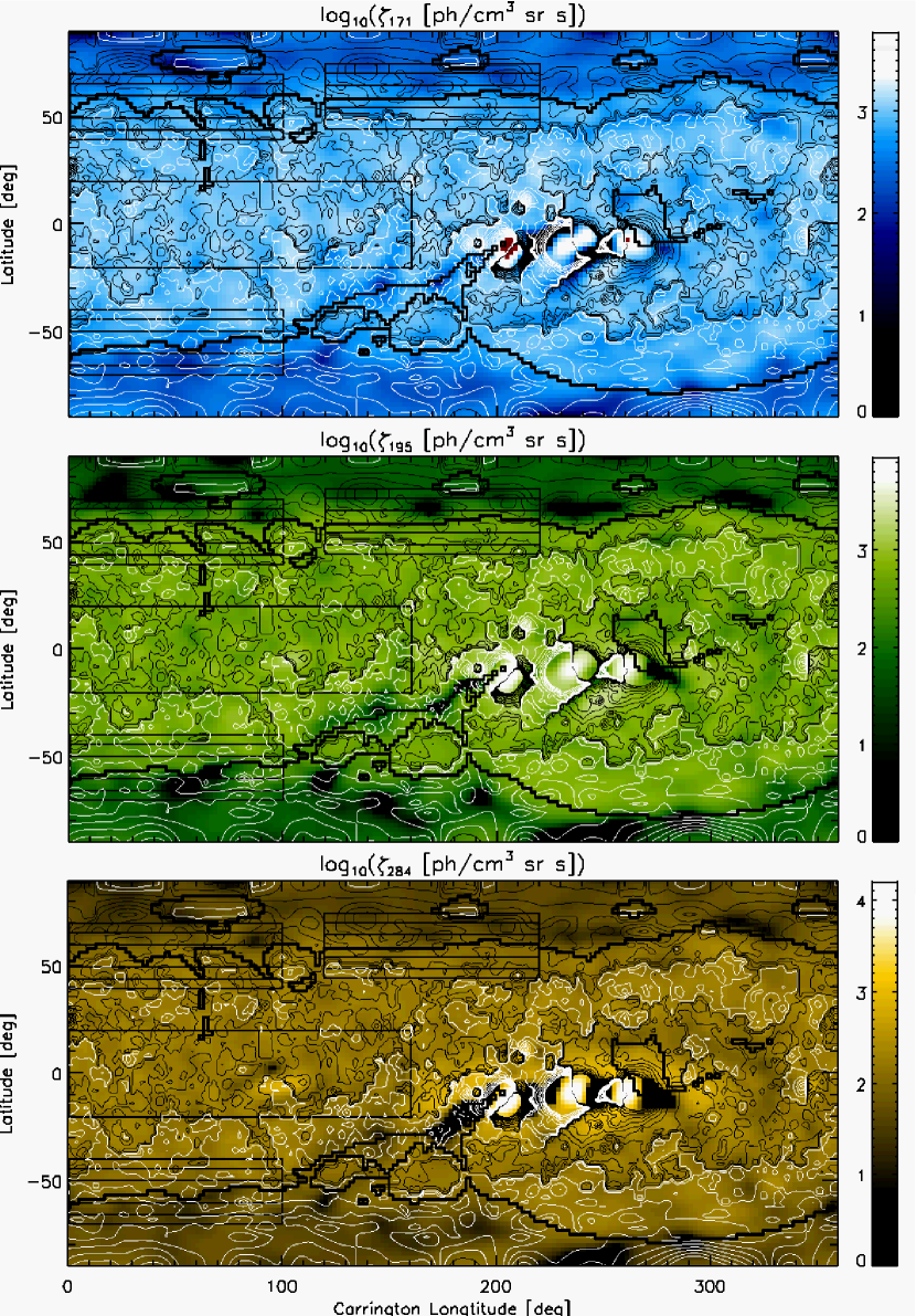
Figure 1.: Carrington maps of the reconstructed 3D FBEs $\zeta_{k}$ at a height of 1.035 $R_{\odot}$, for the three coronal Fe bands at 171, 195, and 284 Å. The overplotted solid-thin curves are magnetic strength [$B$] contour levels from the PFSSM taken at the same height, with those in white (black) representing outward (inward) oriented magnetic field. The solid-thick black curves mark the magnetically open/closed regions boundary. The boxes highlight the regions analyzed in Section resultsC.FBE˙maps˙1

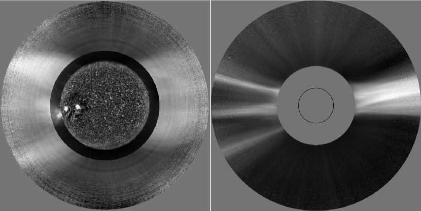
Figure 2.: The solar corona on 2008 March 24, taken from the solar data catalog of the Institute for Astronomy (IfA) of the University of Hawaii (http://alshamess.ifa.hawaii.edu). The images of the different instruments were taken within a fourty minute lapse centered at 19:00 UT. Left: a SOHO EIT 304 Å image, surrounded by a MLSO coronagraph white light image. Right: SOHO LASCO C2 white light image.context

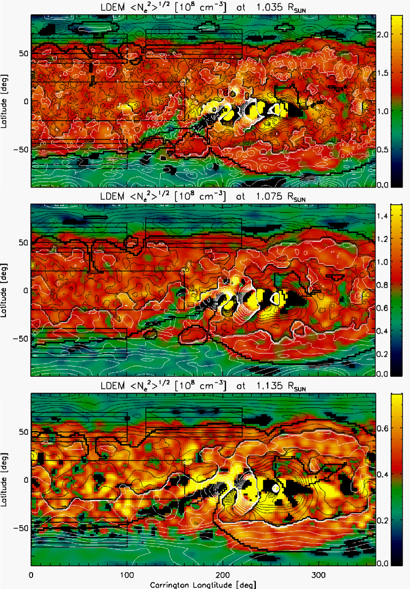
Figure 3.: Carrington maps of the LDEM $\left<N_{e}^{2}\right>^{1/2}$ at heights 1.035, 1.075 and 1.135 $R_{\odot}$, from top to bottom. Solid-thin curves are magnetic strength [$B$] contour levels from the PFSSM taken at the same height, with those in white(black) representing outward(inward) oriented magnetic field. The solid-thick black curves mark the magnetically open/closed regions boundary.LDEM˙Ne˙maps

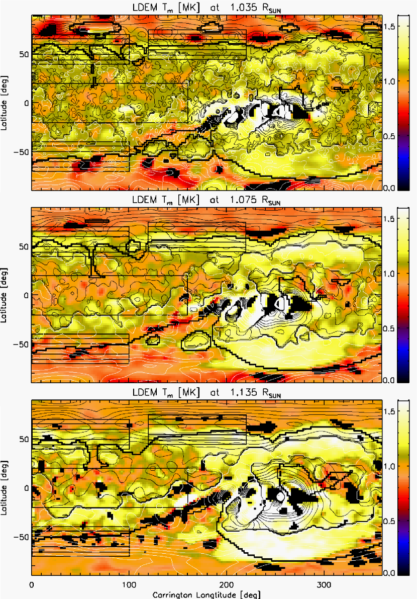
Figure 4.: Carrington maps of the LDEM $T_{\mathrm{m}}$ at heights 1.035, 1.075 and 1.135 $R_{\odot}$, from top to bottom. Solid-thin curves are magnetic strength [$B$] contour levels from the PFSSM taken at the same height, with those in white (black) representing outward (inward) oriented magnetic field. The solid-thick black curves mark the magnetically open/closed regions boundary.LDEM˙Tm˙maps

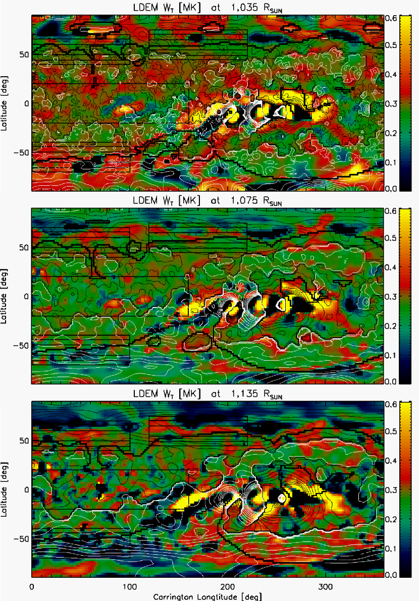
Figure 5.: Carrington maps of the LDEM $W_{T}$ at heights 1.035, 1.075 and 1.135 $R_{\odot}$, from top to bottom. Solid-thin curves are magnetic strength [$B$] contour levels from the PFSSM taken at the same height, with those in white (black) representing outward (inward) oriented magnetic field. The solid-thick black curves mark the magnetically open/closed regions boundary.LDEM˙WT˙maps

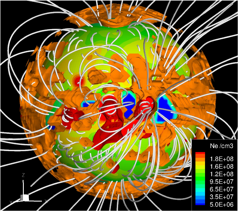
Figure 6.: A 3D view of the CR-2068 PFSS model. Some representative open and closed magnetic-field lines are drawn in white. The red and orange regions are LDEM $T_{\mathrm{m}}$ isosurfaces of 2 and 1 MK, respectively. The inner spherical surface shows the LDEM $N_{\mathrm{e}}$ at 1.04 $R_{\odot}$.3Dview

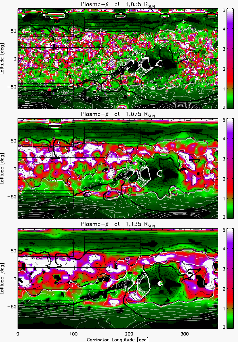
Figure 7.: Carrington maps of the plasma $\beta$ at heights 1.035, 1.075 and 1.135 $R_{\odot}$, from top to bottom. Solid-thin curves are magnetic strength [$B$] contour levels from the PFSSM taken at the same height, with those in white (black) representing outward (inward) oriented magnetic field. The solid-thick black curves mark the magnetically open/closed regions boundary.beta˙maps

Figure 8.: Average dependence with height of the LDEM electron density [$N_{e}(r)$] in the ten regions SC and $R_{i}$-O,B,C of Table 1. The LDEM data is indicated by symbols, while the solid curves show the best hydrostatic fits given by Equation (1). In regions $R_{i}$, the diamonds indicate the closed part of the data inside the streamer, the triangles are the data around the open/closed boundary, and the squares are the data in the open subpolar parts.tomo˙height˙Ne

Figure 9.: Average dependence with height of the LDEM electron mean temperature [$T_{\mathrm{m}}(r)$] in the ten regions SC and $R_{i}$-O,B,C of Table 1. The LDEM data is indicated by symbols, while the solid curves show the best hydrostatic fits given by Equation (1). In regions $R_{i}$, the diamonds indicate the closed part of the data inside the streamer, the triangles are the data around the open/closed boundary, and the squares are the data in the open subpolar parts.tomo˙height˙Tm

Figure 10.: Average dependence with height of the LDEM electron temperature spread [$W_{T}(r)$] in the ten regions SC and $R_{i}$-O,B,C of Table 1. The LDEM data is indicated by symbols, while the solid curves show the best hydrostatic fits given by Equation (1). In regions $R_{i}$, the diamonds indicate the closed part of the data inside the streamer, the triangles are the data around the open/closed boundary, and the squares are the data in the open subpolar parts.tomo˙height˙WT

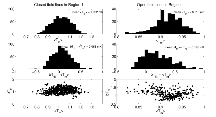
Figure 11.: Statistical analysis of the result of tracing individual closed (left panels) and open (right panels) field lines $i$ in Region $R_{1}$. Top: histograms of $\left<T_{\mathrm{m}}\right>^{(i)}$. Middle: histograms of $bT_{\rm fit}^{(i)}$. Bottom: scatter plots of $bT_{\rm fit}^{(i)}$ versus $\left<T_{\mathrm{m}}\right>^{(i)}$.linetrace˙R1

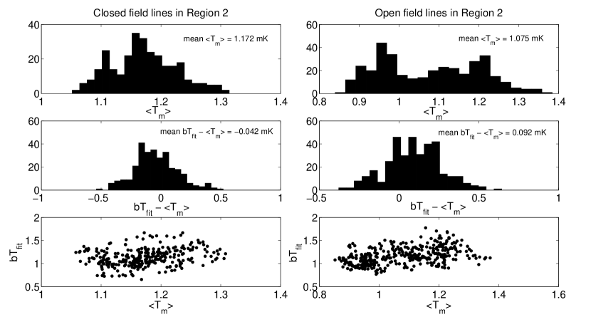
Figure 12.: Statistical analysis of the result of tracing individual closed (left panels) and open (right panels) field lines $i$ in Region $R_{2}$. Top: histograms of $\left<T_{\mathrm{m}}\right>^{(i)}$. Middle: histograms of $bT_{\rm fit}^{(i)}$. Bottom: scatter plots of $bT_{\rm fit}^{(i)}$ versus $\left<T_{\mathrm{m}}\right>^{(i)}$.linetrace˙R2

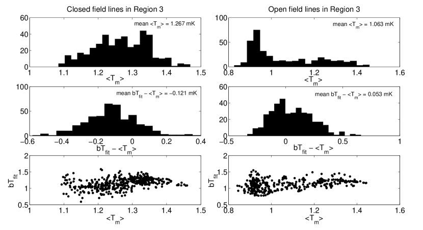
Figure 13.: Statistical analysis of the result of tracing individual closed (left panels) and open (right panels) field lines $i$ in Region $R_{3}$. Top: histograms of $\left<T_{\mathrm{m}}\right>^{(i)}$. Middle: histograms of $bT_{\rm fit}^{(i)}$. Bottom: scatter plots of $bT_{\rm fit}^{(i)}$ versus $\left<T_{\mathrm{m}}\right>^{(i)}$.linetrace˙R3

References

- [1] Altschuler, M.D., Perry, R.M.: 1972, Solar Phys. 23, 410.
- [2] Altschuler, M.D., Levine, R.H., Harvey, J.: 1977, Solar Phys. 51, 345.
- [3] Arnaud, M., Raymond, J.C.: 1992, Astrophys. J. 398, 39.
- [4] Butala, M.D., Hewett, R.J., Frazin, R.A., Kamalabadi, F.: 2010, Solar Phys. 262, 495.
- [5] Feldman, U., Doschek, G.A., Schühle, U., Wilhelm, K.: 1999, Astrophys. J. 518, 500.
- [6] Feldman, U., Mandelbaum, P., Seely, J.L., Doschek, G.A., Gursky, H.: 1992, Astrophys. J. 81, 387.
- [7] Feng, L., Inhester, B., Solanki, S.K., Wilhelm, K., Wiegelmann, T., Podlipnik, B., Howard, R.A., Plunkett, S.P., Wuelser, J.P., Gan, W.Q.: 2009, Astrophys. J. 700, 292.
- [8] Fineschi, S., Gardner, L.D., Kohl, J.L., Romoli, M., Noci, G.C.: 1998, In: Silvano F. (ed.), X-Ray and Ultraviolet Spectroscopy and Polarimetry II Proc. SPIE 3443, SPIE, 67.
- [9] Fisk, L.A.: 2003, J. Geophys. Res. 108, 1157.
- [10] Frazin, R.A., Janzen, P.: 2002, Astrophys. J. 570, 408.
- [11] Frazin, R.A., Kamalabadi, F.: 2005, Solar Phys. 228, 219.
- [12] Frazin, R.A., Kamalabadi, F., Weber, M.A.: 2005, Astrophys. J. 628, 1070.
- [13] Frazin, R.A., Vásquez, A.M., Kamalabadi, F.: 2009, Astrophys. J. 701, 547.
- [14] Galvin, A.B., Popecki, M.A., Simunac, K.D.C., Kistler, L.M., Ellis, L., Barry, J., Berger, L., Blush, L.M., Bochsler, P., Farrugia, C.J., Jian, L.K., Kilpua, E.K.J., Klecker, B., Lee, M., Liu, Y.C.-M., Luhmann, J.L., Moebius, E., Opitz, A., Russell, C.T., Thompson, B., Wimmer-Schweingruber, R.F., Wurz, P.: 2009, Ann. Geophys. 27, 3909.
- [15] Gibson, S.E., Foster, D., Burkepile, J., de Toma, G., Stanger, A.: 2006, Astrophys. J. 641, 590.
- [16] Gibson, S.E., Fludra, A., Bagenal, F., Biesecker, D., Del Zanna, G., Bromage, B.: 1999, J. Geophys. Res. 104, 9691.
- [17] Gloeckler, G., Zurbuchen, T.H., Geiss, J.: 2003, J. Geophys. Res. 108, 1158.
- [18] Grevesse, N., Sauval, A.J.: 1998, Space Sci. Rev. 85, 161.
- [19] Guhathakurta, M., Fisher, R.R.: 1994, Solar Phys. 152, 181.
- [20] Howard, R.A., Moses, J.D., Vourlidas, A., Newmark, J.S., Socker, D.G., Plunkett, S.P., Korendyke, C.M., Cook, J. W., Hurley, A., Davila, J.M., et al.: 2008, Space Sci. Rev. 136, 67.
- [21] Kaiser, M.L., Kucera, T.A., Davila, J.M., St. Cyr, O.C., Guhathakurta, M., Christian, E.: 2008, Space Sci. Rev. 136, 5.
- [22] Kohl, J.L., Esser, R.,Gardner, L.D., Habbal, S., Daigneau, P.S., Dennis, E.F., Nystrom, G.U., Panasyuk, A., Raymond, J.C., Smith, P.L., et al.: 1995, Solar Phys. 162, 313.
- [23] Kohl, J.L., Noci, G., Cranmer, S.R., Raymond, J.C.: 2006, Astron. Astrophys. Rev. 13, 31.
- [24] Landi, E.: 2007, Astroph. J. 663, 1363.
- [25] Levine, R.H., Altschuler, J.W., Harvey, J.W.: 1977, J. Geophys. Res. 82, 1061.
- [26] Li, J., Raymond, J.C., Acton, L.W., Kohl, J.L., Romoli, M., Noci, G., Naletto, G.: 1998, Astrophys. J. 506, 431.
- [27] Manchester IV, W.B., Vourlidas, A., Toth, G., Lugaz, N., Roussev, I.I., Sokolov, I.V., Gombosi, T.I., De Zeeuw, D.L., Opher, M.: 2008, Astrophys. J. 684, 1448.
- [28] Moses, D., Clette, F., Delaboudinière, J.-P., Artzner, G.E., Bougnet, M., Brunaud, J., Carabetian, C., Gabriel, A.H., Hochedez, J.F., Millier, F., et al. 1997, Solar Phys. 175, 571.
- [29] Nerney S., Suess, S.T.: 2005, Astrophys. J. 624,378.
- [30] Phillips, J.L., Bame, S.J., Barnes, A., Barraclough, B.L., Feldman, W.C., Goldstein, B.E., Gosling, J.T., Hoogeveen, G.W., McComas, D.J., Neugebauer, M., Suess, S.T.: 1995, J. Geophys. Res. 22, L3301.
- [31] Raymond, J.C., Kohl, J.L., Noci, G., Antonucci, E., Tondello, G., Huber, M.C. E., Gardner, L.D., Nicolosi, P., Fineschi, S., Romoli, M., et al.: 1997, Solar Phys. 175, 645.
- [32] Raymond, J.C. 1999, Space Sci. Rev. 87, 55.
- [33] Strachan ,L., Suleiman, R., Panasyuk, A.V., Biesecker, D.A., Kohl, J.L.: 2002, Astrophys. J. 571,1008.
- [34] Seely, J.F., Feldman, U., Schuhle, U., Wilhelm, K., Curdt, W., Lemaire, P.: 1997, Astroph. J. 484, L87.
- [35] Suess, S.T., Ko, Y.-K., von Steiger, R., Moore, R.L.: 2009., J. Geophys. Res. 114, A04103.
- [36] Suess, S.T., Wang, A.-H., Wu, S.T.: 1996, J. Geophys. Res. 101, 19957.
- [37] Tu, C.-Y., Marsch, E., Wilhelm, K., Curdt, W.: 1998, Astroph. J. 503, 475.
- [38] Uzzo, M., Strachan, L., Vourlidas, A.: 2007, Astrophys. J. 671, 912.
- [39] Vásquez, A.M., van Ballegooijen, A.A., Raymond, J.C.: 2003, Astrophys. J. 598, 1361.
- [40] Vásquez, A.M., Raymond, J.C.: 2005, Astrophys. J. 619, 1132.
- [41] Vásquez, A.M., Frazin, R.A., Hayashi, K., Sokolov, I.V., Cohen, O., Manchester, W.B., IV, Kamalabadi, F.: 2008, Astrophys. J. 682, 1328.
- [42] Vásquez, A.M., Frazin, R.A., Kamalabadi, F.: 2009, Solar Phys. 256, 73.
- [43] Vásquez, A.M., Frazin, R.A., Manchester IV, W.B.: 2010, Astroph. J. 715, 1352.
- [44] Wang, A.H., Wu, S.T., Suess, S.T., Poletto, G.: 1998, J. Geophys. Res. 103, 1913.
- [45] Wang, Y.-M., Sheeley, N.R., Jr., Walters, J.H., Brueckner, G.E., Howard, R. A., Michels, D.J., Lamy, P.L., Schwenn, R., Simnett, G.M.: 1998, Astrophys. J., 498, L165.
- [46] Wang, Y.-M., Sheeley, N.R., Socker, D.G., Howard, R.A., Rich, N.B.: 2000, J. Geophys. Res., 105, 25133.
- [47] Wilhelm, K., Marsch, E., Dwivedi, B.N., Hassler, D.M., Lemaire, P., Gabriel, A.H., Huber, M.C.E.: 1998, Astrophys. J. 500,1023.
- [48] Wilhelm, K., Inhester, B., Newmark, J.S.: 2002, Astron. Astrophys. 382, 328.